Article
Understanding CollegeApplication Decisions:Why College SportsSuccess Matters
Devin G. Pope1 and Jaren C. Pope2
AbstractUsing a unique, national data set that indicates where students choose to send theirSAT scores, the authors find that college sports success has a large impact onstudent application decisions. For example, a school that has a stellar year in basketballor football on average receives up to 10% more SAT scores. Certain demographicgroups (males, Blacks, out-of-state students, and students who played sports in highschool) are more likely to be influenced by sports success than their counterparts.The authors explore the reasons why students might be influenced by these sportingevents and present evidence that attention/accessibility helps explain these findings.
Keywordscollege sports, school choice, student quality, student demographics
Introduction
Choosing where to apply to college is both an important and complex decision.
Models of college choice typically assume that high school students are fully
informed and choose to apply to and eventually attend a school that maximizes
their expected, present discounted value of future wages less the costs associated
1 University of Chicago, Chicago, IL, USA2 Brigham Young University, Provo, UT, USA
Corresponding Author:
Jaren C. Pope, Brigham Young University, 180 Faculty Office Building, Provo, UT 84602, USA.
Email: [email protected]
Journal of Sports Economics2014, Vol. 15(2) 107-131
ª The Author(s) 2012Reprints and permission:
sagepub.com/journalsPermissions.navDOI: 10.1177/1527002512445569
jse.sagepub.com

with college attendance (Card & Krueger, 2004; Fuller, Manski, & Wise, 1982;
Willis & Rosen, 1979). Thus, variables such as school quality, distance, and tui-
tion should be key predictors of the schools to which students apply and attend.
While this choice problem appears daunting, economists typically argue that due
to the sizable incentives involved, student outcomes should closely approximate
predictions from this rational, decision-making process.
While these classic economic variables are surely important and have been shown
to contain predictive power, it is possible that students are not fully informed
about all potential options and at times use heuristics when making application
decisions. One such case is that students may be more likely to apply to and
attend a college that has recently entered a student’s consideration set due to
an attention-generating event. The degree to which attention/accessibility can
affect the college application process and how the size of these effects relate
to other classic economic variables such as school quality and tuition costs is
an important question since it could provide information on the relative costs
and benefits of providing information to inattentive students.
In this article, we explore the impact of attention in the college application pro-
cess by focusing on college sports. There is little doubt that the media exposure gen-
erated by high-profile college sports such as football and basketball can act as a
powerful advertising tool for institutions of higher education. In fact, one might
expect that future college applicants are much more likely to be aware of a particular
college or university because of the school’s appearance in the ‘‘Final 4’’ of the
National Collegiate Athletic Association’s (NCAA) basketball tournament, rather
than the recent hiring of a world-renowned professor. However, college sports suc-
cess is different from a typical economic variable that predicts college application
decisions since it does not necessarily relate to the quality or cost of the academic
education that a university provides.
In order to evaluate the impact of sports success on college application decisions,
we use an administrative data set from the College Board that records where students
sent their SAT scores—a proxy for where students send their applications. This
unique data set allows us to produce counts for the number and type of students that
send their SAT scores to each college that participates in Division I, NCAA basket-
ball or football. Using a fixed-effects identification strategy that controls for
year- and school-specific unobserved heterogeneity, we find that there is a large and
statistically significant increase in the number of students who send their SAT scores
to schools that perform well in recent basketball or football events. For example, we
find that a school that makes it to the ‘‘Final 4’’ in the NCAA basketball tournament
or is ranked in the top 10 in the Associated Press Poll at the end of the football season
experiences an average increase in sent SAT scores by 6%–8% the following year.
The results we find are robust to including various school-level controls and trends.
Our graphical representation of the results further illustrates how our results are
unlikely to be explained by the endogeneity of sports successes or spurious trends
that can plague this type of analysis.
108 Journal of Sports Economics 15(2)

We argue that the large impact of sports success on student application decisions
is somewhat puzzling, given the classical model of college choice. We posit two key
explanations for our findings. First, it is possible that the standard model is adequate
and that similar to school quality or costs of attendance, college sports success is
simply an important component to a student’s utility function (utility hypothesis).
A second explanation for our findings is that high school students are not fully
informed about potential colleges to which they could apply and that their applica-
tion decisions can be significantly affected by schools that enter their consideration
set via attention-generating events like sports (attention hypothesis). This hypothesis
draws largely on evidence presented in the marketing literature (See for example,
Bain [1956] and Nelson [1974] for a discussion of reasons for advertising and
Roberts and Lattin [1997] and Manrai and Andrews [1998] for reviews of the con-
sideration set literature).
The empirical relationship between sports success and student applications is cer-
tainly interesting and important, independent of the mechanism driving the results.
However, disentangling these two effects is important from a theoretical perspec-
tive. If students are simply placing a large weight on sports success in their utility
function and subsequently optimizing when making application decisions, then there
is little need for changes to current education policy. However, if students are
responding to sports success due to the lack of information about college options,
this may suggest that high school students are not being well guided in their college
application decisions. Increasing the number of guidance counselors and providing
information in other ways may improve student welfare by helping students make
better informed college decisions.
Disentangling these two mechanisms is very difficult and we do not pretend that
our data allow us to identify how much of the sports impact is caused by an attention
effect and how much is caused by a utility effect. Most events that provide a shock to
the attention/accessibility of a school, like sports successes, are likely to impact the
perceived utility of attending that school as well. Even though these two mechanisms
are largely intertwined, we present six pieces of evidence that are, at the very least,
suggestive of the fact that attention could be an important component in application
decisions.
First, the results we present indicate that high school students’ responses to sports
success decay very quickly across time—consistent with a model of inattention. Sec-
ond, we find a larger effect of sports success on out-of-state than for in-state stu-
dents. While a sports victory for a given school may not change the awareness of
in-state students regarding its existence, the sports victory may present a significant
shock in attention/awareness for out-of-state students. Third, we estimate the effect
of women’s basketball success on application decisions. Given the lack of media
attention that women’s basketball receives relative to men’s basketball, one would
expect a smaller effect. Indeed, we find no effect of women’s basketball success
on the number of SAT scores sent to the winning schools. Fourth, using the demo-
graphic information that the SAT data provide, we perform a heterogeneity analysis
Pope and Pope 109

by identifying the impact of sports on SAT score-sending decisions by demographic
subgroupings. We find the influence of sports success on males, Blacks, and students
who played sports in high school to be significantly higher than their counterparts.
Fifth, while certain demographic subgroups are clearly more responsive to sports
success overall, nearly all subgroups become responsive to the most attention-
generating sports victories (e.g., championships). Sixth, we use a regression discon-
tinuity design in the NCAA basketball tournament to measure the impact of barely
winning and thus moving on to receive more attention in later rounds of the tourna-
ment. We find that teams that barely win and thus move on in the tournament are no
more likely to have success in future years relative to teams that barely lost. How-
ever, they receive significantly more applications due to their performance. While a
utility story can be generated that rationalizes each of these findings, we argue that
they are suggestive of attention playing an important role in the college admissions
process and that more work on distinguishing between these two mechanisms is
needed.
Our article relates to a small literature that has previously estimated the effect of
college sports success on college applications. In one of the first papers on the topic,
McCormick and Tinsley (1987) hypothesized that schools with athletic success may
receive more applications, thereby allowing the school to be more selective in the
quality of students they admit. They used data on average SAT scores and in-
conference football winning percentages for 44 schools for the years 1981-1984 and
found some evidence that football success can increase average incoming student
quality. Several follow-up studies have also been conducted and have produced mixed
results (i.e., Bremmer & Kesselring, 1993; Mixon, 1995; Murphy & Trandel, 1994;
Tucker & Amato, 1993). In a recent article (Pope & Pope, 2009), we addressed some
of the data and methodological limitations of previous work and gave clearer evidence
that sports success influences college choice. However, it left many questions about
this process unanswered. This article extends the literature by trying to better explain
which students are influenced by sports success and why this influence occurs.
The article proceeds as follows. In the Conceptual Framework section, we pro-
vide a conceptual framework for college choice and the potential impact of college
sports on application decisions. The Data section describes the data that we use in the
analysis. In the Empirical Strategy section, we outline our empirical strategy. The
Results section presents our results followed by the Discussion and Conclusion
section.
Conceptual Framework
College attendance has been an active area of research in economics and other fields.
Most work in economics assumes that an individual makes their actual application
decisions by comparing the benefits and costs of all possible alternatives and
chooses to apply to the schools that maximize overall utility (Card & Krueger,
110 Journal of Sports Economics 15(2)

2004; Fuller et al., 1982; Willis & Rosen, 1979).1 However, a significant amount of
work has focused on providing a richer context for college application decisions. For
example, Perna (2006) argues that ‘‘when considered separately, neither rational
human capital investment models nor sociological approaches are sufficient for
understanding differences across groups in student college choice.’’ Manski
(1993) also discusses this point. He argues that economic approaches are limited
by failing to assess the importance of available information on decisions while
sociologic approaches fail to identify how decisions are made once information
is gathered. In her review, Perna (2006) concludes that ‘‘. . . college choice is ulti-
mately based on a comparison of the benefits and costs of enrolling, assessments
of the benefits and costs are shaped not only by demand for higher education and
supply of resources to pay the costs but also by an individual’s habitus and,
directly and indirectly, by the family, school, and community context, higher edu-
cation context, and social, economic, and policy context. By drawing on con-
structs from both human capital and sociological approaches, the proposed
conceptual model will likely generate a more comprehensive understanding of
student college choice.’’
Below we provide a simple framework that attempts to combine utility maximi-
zation with a more thorough understanding of the search process. Hossler and Gal-
lagher (1987) provide a well-used framework for the search process. They argue that
college-choice decisions follow three general stages: (i) Predisposition: deciding
whether to continue formal education beyond secondary education; (ii) Search:
understanding and searching for college attributes that will affect their choice; and
(iii) Choice: constructing a set of schools to apply to and then choosing a school to
attend. Most models are essentially reduced-form approximations of the predisposi-
tion and choice stages. In fact, a substantial amount of work has been done by
researchers in the field of higher education on these two stages (Hossler, Braxton,
and Coopersmith [1989] provides a dated but useful review of this literature). Much
less has been done on understanding the search stage of the college choice process.
By acknowledging that search costs and limited awareness make it unlikely that high
school students consider all possible colleges when making their decisions about
where to apply, the framework that we outline essentially includes elements of the
search stage as well.
In this article, we assume that increasing college sports success weakly increases
the utility that a high school student assigns to attending that school.2 Thus, sports
success can increase student applications through the utility channel. Furthermore,
sports success weakly increases the exposure that a student has to a given college
which can increase student applications through the attention channel.3 For example,
the better a sports team performs, the more applications its school will receive (mak-
ing it to the Final 4 is better than only making it to the Final 64). Demographic
groups that on average care the most about sports (e.g., males, people who played
sports in high school, etc.) will be affected the most. Lower profile sports will have
a smaller effect on application rates than higher profile sports (e.g., women’s
Pope and Pope 111

basketball success should have less of an impact than men’s basketball success). All
of these predictions can be utility- or attention-driven.4 In our results, we look for
situations where intuition suggests that attention is the primary channel and we look
to see if SAT score sending continues to be responsive in these situations.
Data
SAT Data
The data used in this analysis are obtained from the College Board’s Test Takers
Database (referred to as SAT database in the remainder of the article).5 The data
are at the individual level and represent a 25% random sample of all SAT test-
takers nationwide with high school graduation dates between 1994 and 2001. It
also includes a 100% sample of SAT test-takers that are Californians, Texans,
African American, or Hispanic. The data are classified by cohorts according to
the year in which the students are expected to graduate. For example, the 1994
cohort group contains students who took the SAT who are expected to graduate
in the spring of 1994 and apply to begin college the following fall. The SAT data-
base provides demographic and other background information in the Student
Descriptive Questionnaire component of the SAT. The data report the SAT score
and background characteristics of the most recent test and survey taken. For most
students, this is at the beginning of their senior year in high school. The data set
identifies the first 20 schools to which a student has requested his or her scores be
sent.6 The median number of schools to which a student requested his scores be
sent was 5 across all years in our sample. We restrict the data to students who
sent their scores to at least one of the 332 schools that played NCAA Division
I basketball or Division I-A football.7 We also weight the observations so that the
data are representative of all SAT-taking, potential college applicants to each of
these 332 schools.8
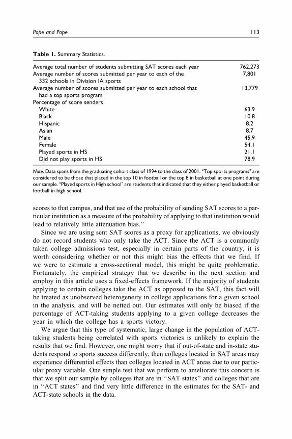
Table 1 presents summary statistics for the data. The table shows that schools
that participate in Division I sports receive on average 7,801 SAT scores each
year. Schools that have done well in sports (those in the top 10 in football or
top 8 in basketball at some time between 1994 and 2001) are typically larger
schools and receive more SAT scores—13,779 on average. These numbers will
be useful when interpreting the size of the results we find later in the article.
In this article, we use sending a SAT score as a proxy for applying to a school.
Using this same SAT test-takers data set, Card and Krueger (2004) tested the validity
of using sent SAT scores as a proxy for applications. They compared the number of
SAT scores that students of different ethnicities sent with admissions records from
California and Texas, to administrative data on the number of applications received
by ethnicity. They conclude that ‘‘trends in the number of applicants to a particular
campus are closely mirrored by trends in the number of students who send their SAT
112 Journal of Sports Economics 15(2)
scores to that campus, and that use of the probability of sending SAT scores to a par-
ticular institution as a measure of the probability of applying to that institution would
lead to relatively little attenuation bias.’’
Since we are using sent SAT scores as a proxy for applications, we obviously
do not record students who only take the ACT. Since the ACT is a commonly
taken college admissions test, especially in certain parts of the country, it is
worth considering whether or not this might bias the effects that we find. If
we were to estimate a cross-sectional model, this might be quite problematic.
Fortunately, the empirical strategy that we describe in the next section and
employ in this article uses a fixed-effects framework. If the majority of students
applying to certain colleges take the ACT as opposed to the SAT, this fact will
be treated as unobserved heterogeneity in college applications for a given school
in the analysis, and will be netted out. Our estimates will only be biased if the
percentage of ACT-taking students applying to a given college decreases the
year in which the college has a sports victory.
We argue that this type of systematic, large change in the population of ACT-
taking students being correlated with sports victories is unlikely to explain the
results that we find. However, one might worry that if out-of-state and in-state stu-
dents respond to sports success differently, then colleges located in SAT areas may
experience differential effects than colleges located in ACT areas due to our partic-
ular proxy variable. One simple test that we perform to ameliorate this concern is
that we split our sample by colleges that are in ‘‘SAT states’’ and colleges that are
in ‘‘ACT states’’ and find very little difference in the estimates for the SAT- and
ACT-state schools in the data.
Table 1. Summary Statistics.
Average total number of students submitting SAT scores each year 762,273Average number of scores submitted per year to each of the
332 schools in Division IA sports7,801
Average number of scores submitted per year to each school thathad a top sports program
13,779
Percentage of score sendersWhite 63.9Black 10.8Hispanic 8.2Asian 8.7Male 45.9Female 54.1Played sports in HS 21.1Did not play sports in HS 78.9
Note. Data spans from the graduating cohort class of 1994 to the class of 2001. ‘‘Top sports programs’’ areconsidered to be those that placed in the top 10 in football or the top 8 in basketball at one point duringour sample. ‘‘Played sports in High school’’ are students that indicated that they either played basketball orfootball in high school.
Pope and Pope 113

Sports Data
We gathered sports data on NCAA basketball and football success for all 332
schools that participate in NCAA Division I basketball or Division I-A Football.
We use the Associated Press’s college football poll as our indicator of football suc-
cess. This poll ranks NCAA division I-A football teams based upon game perfor-
mances throughout the year. We collected the end of season rankings for
teams finishing in the top 20 between the years 1991 and 2001.9 Although this
indicator does not incorporate all measures of success (e.g., big wins against key
rivals, an exciting individual player on a team, etc.), it probably proxies these
indicators for the top 20 teams each year.
For basketball success, we gather data on team performance in the NCAA
men’s college basketball tournament. It is widely agreed that this tournament
provides the greatest media exposure and indicator of success for a college bas-
ketball team (particularly on a national level) each year. ‘‘March Madness’’ as it
is often called takes place at the end of the college basketball season in March
and the beginning of April. It is a single elimination tournament that determines
who wins the college basketball championship. Since 1985, 64 teams have been
invited to play each year.10 We collected information on all college basketball
teams that were invited to the tournament between 1991 and 2001. From these
data, we create four dummy variables that indicate the furthest round in which a
team played: rounds of 64, 16, 4, and champion. We also gathered similar data
for women’s teams that advanced to the Final 4 and championship games in the
women’s basketball tournament.
In order to better interpret the results, it is important to understand
exactly where the variation in sports success is coming from. Of the 332 schools
that play Division I-A basketball or football, 145 (44.8%) were never invited
to participate in the NCAA Tournament. Given the fixed-effects framework that
we use and describe below, these schools will not provide any variation leading
to the results that we find for the impact of basketball success on score sending.
However, the majority of Division IA schools (187) will provide variation in our
analysis. Of these 187 schools, 62 of them made it to the Tournament just once,
48 twice, 21 three times, and so on. Only nine schools (2.8%) participated in the
Tournament every year in our data. Since we will be identifying effects for dif-
ferent levels of success within the Tournament (advancing to the round of 16, 4,
etc.), even these nine schools provide variation for our analysis since no school
advanced to the exact same round in all years.
For football, 51 of the 101 schools that participated during our sample ended
the season in the top 20 at some point during our sample. 15 teams did so just
once, 13 teams twice, 8 teams three times, and so on. Only three schools (3%)
finished in the top 20 all eight seasons. Like basketball, the variation that we use
in our analysis will come from the 51 teams that at some point finished in the
top 20.
114 Journal of Sports Economics 15(2)

Empirical Strategy
Specification
Many school characteristics cannot be observed by the econometrician, yet these
unobservables are likely correlated with both indicators of sports success and the
number of applications received by a school. The unobservable component is likely
to include information about scholastic tradition, geographic advantages, and other
information on the quality of the school. Without adequately controlling for these
unobservables, they would likely confound the ability to detect the impact of athletic
success on student applications.
Previous studies have pointed to a large number of institutional characteristics
that impact college-choice decisions such as tuition, financial aid, location, reputa-
tion, selectivity, special programs, and curriculum (see e.g., Abraham & Clark,
2006; DesJardins, Ahlburg, & McCall, 2006; Dynarski, 2000). The nature of the data
we have compiled and the econometric specification that we employ takes advan-
tage of the panel design of the data and thereby is able to control for the stationary
aspects of a school (e.g., location, curriculum). We use a fixed-effects model where
the fixed effects control for year-specific and school-specific unobserved heteroge-
neity. We also include a linear trend for each school to try to capture heterogeneous
trend rates. We include several additional variables on the right-hand side of the
equation to further control for quality characteristics of the schools that change
across time. The econometric specification we use is the following,
Yji;t ¼ ai;t þ tli þ Si;tbþ Si;t�1dþ Si;t�2gþ Si;t�3yþ Xi;tfþ ei;t; ð1Þ
where Yji;t represents the log number of SAT scores sent to school i in year t from the
jth population group. The key covariate Si;t is a vector of dummy variables indicating
the level of sports success that school i had during year t. We include up to three lags
for each sports variable in our model in order to examine persistence in the effects of
a winning season on applications. School- and year-fixed effects are included along
with a linear time trend for each school. Xi;t is a set of four control variables com-
monly used in the literature to control for the quality of the school—log total cost
to attend school, log average professor salary (lagged one year), log average real
income in the state in which the school is located, and the number of public high
school diplomas awarded in the state in which the school is located during year t.11
Lag Structure
Understanding when prospective students apply to college in relation to the football
and basketball seasons is crucial in determining which lags of our athletic success
variables should affect the left-hand side of Equation 1. Fall admission application
deadlines vary by school. They can occur any time between November and August
before the expected fall enrollment period. Furthermore, students often have to send
letters of recommendation and SAT scores to the school well before the actual
Pope and Pope 115

deadlines. Figure 1 illustrates the distribution of application deadlines for our sample
of schools in 2003. The label ‘‘continuous’’ in Figure 1 refers to those schools that
have a rolling application period rather than a specific deadline. The NCAA Division
I-A football season finishes at the beginning of January. The NCAA basketball tour-
nament finishes at the end of March or beginning of April. Therefore, since Figure 1
illustrates that about half of the schools in our sample have application deadlines
after April, we might expect some effect on the current year variables. This means
that a successful football team that finishes in January or a successful basketball
team that finishes in March may still influence application decisions for students
enrolling that upcoming fall. However, given the timing of when applications are
likely prepared and submitted, one would expect athletic success to have its largest
impact when lagged one period (especially for basketball which is 3 months after
football). The second and third lags should provide an indication of the persistence
of the effect that athletic success has on application rates.
Regression Discontinuity Design
We implement a regression-discontinuity design to analyze the effect of two teams
that in a given season show equal sports competence, but receive different levels of
attention. It is plausible that teams that just win a NCAA basketball tournament
game have similar capabilities to those that just lose. Thistlethwaite and Campbell
0
20
40
60
80
100
120
Num
ber o
f Sch
ools
Month of Application Deadline
Football
Season
Ends
Basketball
Season
Ends
Figure 1. Application deadlines. Note. The figure includes all schools that compete in DivisionI football or basketball. Application deadline data are based on 2003 information from alicensed data set from Peterson’s (a part of the Thompson Corporation).
116 Journal of Sports Economics 15(2)

(1960) first proposed using an observed discontinuity to estimate causal effects.
Nonetheless, the presence of an observed discontinuity does not guarantee one can
estimate a causal effect. The identifying assumption in our case is that all observable
and unobservable pre-event characteristics between the winning and losing teams
are not systematically different. For example, it is possible that better teams have the
ability to perform at a higher level at the end of games and therefore, even very close
games are usually won by the better team. If this is the case, it is not possible to
establish a causal relationship using this discontinuity. Ultimately, it is necessary
to look at the observable data to generate a convincing argument that the winners
and losers are equivalent ex ante.
To make this ex ante comparability argument, we present two pieces of graphical
evidence. First, we gather data on the seed of each team in the tournament.12 We
examine whether or not a discontinuity exists in team seed at the point of just
‘‘barely’’ winning the game. If barely winning is not random, then we might find
a significant discontinuity in the average seed for teams that just barely lost com-
pared to teams that just barely won (e.g., better teams are able to ‘‘step it up’’ when
a game is close). We also examine whether or not a discontinuity exists in the prob-
ability that a team makes it to the NCAA tournament the following year based on
whether they barely won or lost in the current year. After analyzing these two tests,
we run our baseline regression and compare the increase in number of SAT senders
for teams that barely won and teams that barely lost and compare the difference in
coefficients.
Results
Overall Results
The main effects with robust standard errors clustered at the school level are pre-
sented in Table 2. Column 1 of Table 2 provides the results using all of the data.
We find that being one of the 64 teams in the NCAA tournament yields a 2.2%increase in the total number of SAT score senders the following year, making it
to the ‘‘sweet 16’’ yields a 3.8% increase, making it to the ‘‘Final 4’’ a 5.7% increase,
and being the champion a 9% increase. For football, the results suggest that ending
the season ranked in the top 20 results in a 2% increase in score senders the following
year, ending in the top 10 yields a 5.2% increase, and ending as the football cham-
pion yields an 11% increase in score senders the following year. All but one of these
effects is statistically significant at the 1% confidence level.
Looking across the columns in Table 2, we find very distinct responses to athletic
success from different groups of students. Blacks are roughly twice as responsive to
basketball success as any other race. For example, making it into the Final 4 yields a
13% increase in Black SAT scores sent (SE ¼ 3.2%) compared to a 5.7% increase
(SE ¼ 1.5%) for the overall population. The basketball champion in a given year
Pope and Pope 117

Tab
le2.
The
Impac
tofSu
cces
sin
Men
’sBas
ketb
allan
dFo
otb
allon
SAT
Score
Sendin
g.
Dep
enden
tV
aria
ble
:Lo
gN
um
ber
ofSA
TSc
ore
sSe
nt
by
Subgr
oup
Eve
ryone
White
Bla
ckH
ispan
icA
sian
Mal
esFe
mal
esSp
ort
sN
oSp
ort
sIn
-Sta
teO
ut-
of-
Stat
e
Bas
ketb
all
Final
_64_lg
10.0
22**
(0.0
06)
0.0
24*
(0.0
11)
0.0
40**
(0.0
12)
0.0
16
(0.0
16)
�0.0
02
(0.0
28)
0.0
28**
(0.0
07)
0.0
15
(0.0
08)
0.0
41**
(0.0
09)
0.0
15*
(0.0
06)
0.0
19
(0.0
12)
0.0
28**
(0.0
09)
Final
_16_lg
10.0
38**
(0.0
10)
0.0
39**
(0.0
11)
0.0
91**
(0.0
22)
0.0
17
(0.0
19)
0.0
17
(0.0
30)
0.0
42**
(0.0
13)
0.0
40**
(0.0
13)
0.0
69**
(0.0
14)
0.0
26*
(0.0
11)
0.0
31*
(0.0
15)
0.0
54**
(0.0
13)
Final
_4_lg
10.0
57**
(0.0
15)
0.0
54**
(0.0
16)
0.1
30**
(0.0
32)
0.0
69*
(0.0
32)
0.0
61
(0.0
61)
0.0
66**
(0.0
17)
0.0
52**
(0.0
19)
0.0
75**
(0.0
14)
0.0
51**
(0.0
17)
0.0
45**
(0.0
16)
0.0
72**
(0.0
20)
Cham
p_lg
10.0
90**
(0.0
31)
0.0
90**
(0.0
33)
0.1
88**
(0.0
49)
0.0
79
(0.0
73)
0.0
94
(0.0
67)
0.0
88**
(0.0
26)
0.1
01*
(0.0
43)
0.1
07**
(0.0
40)
0.0
86**
(0.0
31)
0.0
92
(0.0
52)
0.0
93**
(0.0
30)
Footb
all
Top_20_lg
10.0
20*
(0.0
10)
0.0
23
(0.0
15)
0.0
42*
(0.0
21)
0.0
51**
(0.0
17)
0.0
28
(0.0
28)
0.0
27*
(0.0
12)
0.0
14
(0.0
12)
0.0
35*
(0.0
14)
0.0
16
(0.0
11)
0.0
09
(0.0
19)
0.0
28
(0.0
15)
Top_10_lg
10.0
52**
(0.0
09)
0.0
52**
(0.0
11)
0.0
66**
(0.0
22)
0.0
76**
(0.0
19)
0.0
29
(0.0
27)
0.0
62**
(0.0
11)
0.0
42**
(0.0
11)
0.0
65**
(0.0
13)
0.0
48**
(0.0
10)
0.0
11
(0.0
17)
0.0
74**
(0.0
11)
Cham
p_lg
10.1
10**
(0.0
12)
0.1
08**
(0.0
16)
0.1
85**
(0.0
64)
0.1
79**
(0.0
58)
0.0
42
(0.0
48)
0.1
26**
(0.0
24)
0.0
95**
(0.0
26)
0.1
48**
(0.0
20)
0.0
98**
(0.0
13)
0.0
63**
(0.0
19)
0.1
50**
(0.0
17)
SchoolF.
E.s
XX
XX
XX
XX
XX
XY
ear
F.E.s
XX
XX
XX
XX
XX
XSc
hooltr
ends
XX
XX
XX
XX
XX
XSc
hoolco
ntr
ols
XX
XX
XX
XX
XX
XO
bse
rvat
ions
2,4
31
2,4
27
2,4
29
2,4
26
2,4
11
2,4
30
2,4
29
2,4
28
2,4
31
2,4
19
2,4
30
R2
.997
.995
.994
.993
.981
.996
.997
.994
.997
.995
.996
Sport
R2
.021
.009
.029
.007
.001
.022
.014
.027
.014
.004
.019
Not
e.R
obust
stan
dar
der
rors
clust
ered
atth
esc
hooll
evel
are
pre
sente
din
par
enth
eses
.Contr
olv
aria
ble
sth
atar
ein
cluded
are
school-
and
year
-fix
edef
fect
s,sc
hool�
year
(lin
ear
tren
ds)
,num
ber
ofhig
hsc
hoold
iplo
mas
give
nout
that
year
inth
esc
hool’s
stat
e,lo
gav
erag
epro
fess
or
sala
ry,l
og
aver
age
real
inco
me
inth
esc
hool’s
stat
e,an
dlo
gtu
itio
nco
st.S
port
R2
isth
efr
action
ofsc
ore
-sen
din
gva
riat
ion
afte
rco
ntr
olli
ng
for
fixed
effe
cts,
tren
ds,
and
schoolc
ontr
ols
that
can
be
expla
ined
by
the
sport
sva
riab
les.
*Sig
nifi
cant
at5%
.**
Sign
ifica
nt
at1%
.
118

receives on average 18.8% more Black SAT scores the following year. Hispanics
and Blacks are the two races most likely to be affected by football success. Asians
are the least likely to be affected by both basketball and football. The results indicate
that males respond more to sports success than females. Similarly, the coefficients
on the students who played basketball or football in high school are generally at least
twice as large as those of students who did not play sports. These findings can be
broken down even further. For example, we have looked at the responsiveness of
female, non-sports students to college sports success. As expected, the effects for
this subgroup are even smaller (however, still significant for the Final 4 and cham-
pion in basketball and Top 10 and champion in football). Both out-of-state and in-
state students are affected by sports success, but there is a larger average effect for
out-of-state students.
(Tables 2 and 3) report two different R2 values. The first is the standard R2 that
indicates that our model fits the data very well (over 99% of the variation in score
sending can be explained by our model). Of course, most of this explained variation
comes from the school- and year-fixed effects as well as the school trends and con-
trols. One may also be interested in how much of the remaining variation in score
sending (after letting fixed effects, trends, and school controls soak up what variation
they can) is explained by our sports success variables. This is what is reported as
Sport R2 in the Tables. For example, the first column in Table 2 indicates that
2.1% of the variation in score sending that remains after all of the other variables
are controlled for in our analysis can be explained by sports success.
An important question about these effects is whether they persist across a long
period of time. In Table 3 and in Figures 2 and 3, we provide information about the
dynamics of this process. While Table 3 provides exact results and standard errors,
we will focus on the results that are presented in Figures 2 and 3 which we find easier
to digest. The coefficient values and robust standard error bars are presented for the
effect of current year sports success on SAT scores sent (the open diamonds), while
the closed circles, open circles, and open squares indicate the effects of sports success
lagged by 1, 2, and 3 years, respectively. The top panel in Figure 2 indicates the coef-
ficient values for making it into the NCAA basketball tournament (round of 64). The
other panels in Figure 2 and Figure 3 present the coefficient values for achieving the
different levels of sports success that we have discussed. Column 1 presents the effect
of sports success on the log number of total SAT senders. Subsequent columns present
the effect of sports success on the log number of SAT senders in different subgroups.
As was expected, there appears to be some effect on the current football sports
variables (the football season ends three months before the basketball season) but
little effect on the current basketball sports variables. The effects are large and sig-
nificant on the first and second lags, while by the third lag the effects are usually
diminished to a small magnitude and are insignificant. These results suggest that the
better the sports team performs, the more applications a college will receive in the
year or two following the sports victory, but that these effects fade away fairly
quickly.
Pope and Pope 119

Tab
le3.
The
Impac
tofSu
cces
sin
Men
’sBas
ketb
allan
dFo
otb
allon
SAT
Score
Sendin
g—La
gSt
ruct
ure
.
Dep
enden
tV
aria
ble
:Lo
gN
um
ber
ofSA
TSc
ore
sSe
nt
by
Subgr
oup
Eve
ryone
White
Bla
ckH
ispan
icA
sian
Mal
esFe
mal
esSp
ort
sN
oSp
ort
sIn
-Sta
teO
ut-
of-
Stat
e
A.Bas
ketb
all
Final
_64
0.0
04
(0.0
08)
0.0
12
(0.0
13)
0.0
19
(0.0
14)
0.0
10
(0.0
17)
�0.0
22
(0.0
28)
0.0
03
(0.0
09)
0.0
06
(0.0
08)
0.0
17
(0.0
10)
0.0
01
(0.0
08)
0.0
03
(0.0
12)
0.0
05
(0.0
11)
Final
_64_lg
10.0
24**
(0.0
07)
0.0
29*
(0.0
11)
0.0
50**
(0.0
15)
0.0
16
(0.0
19)
�0.0
08
(0.0
28)
0.0
31**
(0.0
08)
0.0
16
(0.0
09)
0.0
50**
(0.0
11)
0.0
15
(0.0
08)
0.0
22
(0.0
13)
0.0
27*
(0.0
11)
Final
_64_lg
20.0
15*
(0.0
07)
0.0
16
(0.0
09)
0.0
39
(0.0
21)
0.0
08
(0.0
20)
�0.0
10
(0.0
27)
0.0
20*
(0.0
08)
0.0
11
(0.0
11)
0.0
31*
(0.0
13)
0.0
08
(0.0
08)
0.0
17
(0.0
09)
0.0
07
(0.0
11)
Final
_64_lg
3�
0.0
01
(0.0
08)
0.0
07
(0.0
08)
0.0
11
(0.0
15)
�0.0
11
(0.0
15)
0.0
00
(0.0
25)
0.0
02
(0.0
09)
�0.0
04
(0.0
09)
0.0
08
(0.0
11)
�0.0
04
(0.0
08)
0.0
05
(0.0
11)
�0.0
09
(0.0
10)
Final
_16
0.0
11
(0.0
11)
0.0
20
(0.0
11)
�0.0
08
(0.0
27)
0.0
35
(0.0
25)
�0.0
20
(0.0
48)
0.0
13
(0.0
12)
0.0
05
(0.0
16)
0.0
24
(0.0
15)
0.0
08
(0.0
11)
0.0
15
(0.0
17)
0.0
07
(0.0
14)
Final
_16_lg
10.0
48**
(0.0
13)
0.0
52**
(0.0
14)
0.1
04**
(0.0
23)
0.0
24
(0.0
24)
0.0
19
(0.0
36)
0.0
54**
(0.0
16)
0.0
47**
(0.0
15)
0.0
86**
(0.0
16)
0.0
34*
(0.0
14)
0.0
43*
(0.0
18)
0.0
65**
(0.0
16)
Final
_16_lg
20.0
42**
(0.0
14)
0.0
43**
(0.0
15)
0.0
78**
(0.0
27)
�0.0
06
(0.0
30)
0.0
29
(0.0
37)
0.0
52**
(0.0
15)
0.0
33*
(0.0
15)
0.0
52**
(0.0
19)
0.0
38**
(0.0
14)
0.0
38*
(0.0
17)
0.0
52**
(0.0
17)
Final
_16_lg
30.0
11
(0.0
11)
0.0
17
(0.0
12)
0.0
43*
(0.0
21)
0.0
20
(0.0
24)
0.0
06
(0.0
32)
0.0
13
(0.0
12)
0.0
08
(0.0
12)
0.0
19
(0.0
13)
0.0
10
(0.0
11)
0.0
21
(0.0
13)
0.0
07
(0.0
15)
Final
_4
0.0
19
(0.0
17)
0.0
19
(0.0
18)
0.0
37
(0.0
30)
0.0
26
(0.0
30)
�0.0
09
(0.0
48)
0.0
20
(0.0
18)
0.0
16
(0.0
21)
0.0
13
(0.0
17)
0.0
21
(0.0
19)
0.0
29
(0.0
31)
0.0
17
(0.0
19)
Final
_4_lg
10.0
58**
(0.0
14)
0.0
57**
(0.0
16)
0.1
43**
(0.0
33)
0.0
79*
(0.0
31)
0.0
56
(0.0
62)
0.0
71**
(0.0
14)
0.0
47*
(0.0
22)
0.0
87**
(0.0
18)
0.0
49**
(0.0
16)
0.0
49*
(0.0
24)
0.0
74**
(0.0
18)
Final
_4_lg
20.0
28*
(0.0
14)
0.0
24
(0.0
17)
0.1
13**
(0.0
39)
0.0
08
(0.0
30)
0.0
34
(0.0
33)
0.0
45*
(0.0
19)
0.0
13
(0.0
17)
0.0
75**
(0.0
19)
0.0
12
(0.0
15)
0.0
20
(0.0
28)
0.0
39*
(0.0
19)
Final
_4_lg
30.0
08
(0.0
18)
0.0
15
(0.0
23)
0.0
35
(0.0
27)
0.0
12
(0.0
29)
�0.0
07
(0.0
57)
0.0
19
(0.0
19)
�0.0
04
(0.0
20)
0.0
26
(0.0
23)
0.0
03
(0.0
18)
0.0
25
(0.0
37)
0.0
05
(0.0
18)
Cham
p0.0
05
(0.0
23)
�0.0
01
(0.0
26)
0.0
39
(0.0
34)
0.0
49
(0.0
41)
�0.0
60
(0.0
41)
0.0
22
(0.0
31)
�0.0
22
(0.0
26)
�0.0
08
(0.0
22)
0.0
10
(0.0
27)
0.0
18
(0.0
26)
�0.0
16
(0.0
36)
Cham
p_lg
10.1
09**
(0.0
34)
0.1
01**
(0.0
35)
0.2
33**
(0.0
50)
0.1
41*
(0.0
59)
0.1
13
(0.0
63)
0.1
15**
(0.0
35)
0.1
10**
(0.0
42)
0.1
18**
(0.0
43)
0.1
09**
(0.0
36)
0.1
11*
(0.0
53)
0.1
02**
(0.0
35)
Cham
p_lg
20.0
84*
(0.0
39)
0.0
67
(0.0
36)
0.1
90**
(0.0
56)
0.0
93**
(0.0
35)
0.1
48
(0.0
91)
0.1
07*
(0.0
47)
0.0
68
(0.0
44)
0.0
78*
(0.0
34)
0.0
87*
(0.0
44)
0.0
69
(0.0
36)
0.0
82
(0.0
49)
(con
tinue
d)
120

Tab
le3.
(continued
)
Dep
enden
tV
aria
ble
:Lo
gN
um
ber
ofSA
TSc
ore
sSe
nt
by
Subgr
oup
Eve
ryone
White
Bla
ckH
ispan
icA
sian
Mal
esFe
mal
esSp
ort
sN
oSp
ort
sIn
-Sta
teO
ut-
of-
Stat
e
Cham
p_lg
30.0
26
(0.0
32)
0.0
05
(0.0
36)
0.1
02*
(0.0
47)
0.0
46
(0.0
46)
0.0
15
(0.0
55)
0.0
34
(0.0
40)
0.0
21
(0.0
34)
0.0
39
(0.0
25)
0.0
23
(0.0
36)
0.0
57*
(0.0
27)
0.0
01
(0.0
42)
B.Fo
otb
all
Top_20
0.0
10
(0.0
11)
0.0
14
(0.0
12)
�0.0
07
(0.0
20)
0.0
06
(0.0
24)
�0.0
27
(0.0
37)
0.0
18
(0.0
11)
0.0
06
(0.0
16)
0.0
15
(0.0
13)
0.0
10
(0.0
12)
0.0
32
(0.0
17)
0.0
03
(0.0
16)
Top_20_lg
10.0
26*
(0.0
12)
0.0
28
(0.0
18)
0.0
39
(0.0
23)
0.0
57**
(0.0
21)
0.0
35
(0.0
30)
0.0
34**
(0.0
12)
0.0
20
(0.0
15)
0.0
44**
(0.0
15)
0.0
21
(0.0
13)
0.0
18
(0.0
20)
0.0
33
(0.0
18)
Top_20_lg
20.0
22*
(0.0
09)
0.0
21
(0.0
13)
0.0
01
(0.0
21)
0.0
49
(0.0
30)
0.0
41
(0.0
30)
0.0
30*
(0.0
13)
0.0
16
(0.0
12)
0.0
34*
(0.0
17)
0.0
19
(0.0
11)
0.0
21*
(0.0
10)
0.0
27
(0.0
15)
Top_10
0.0
22*
(0.0
09)
0.0
22
(0.0
11)
0.0
05
(0.0
20)
0.0
45
(0.0
28)
0.0
18
(0.0
27)
0.0
27*
(0.0
11)
0.0
16
(0.0
10)
0.0
24*
(0.0
11)
0.0
22*
(0.0
10)
0.0
12
(0.0
13)
0.0
24
(0.0
12)
Top_10_lg
10.0
60**
(0.0
11)
0.0
59**
(0.0
12)
0.0
77**
(0.0
27)
0.0
91**
(0.0
19)
0.0
40
(0.0
29)
0.0
72**
(0.0
13)
0.0
48**
(0.0
12)
0.0
72**
(0.0
14)
0.0
56**
(0.0
11)
0.0
12
(0.0
17)
0.0
84**
(0.0
14)
Top_10_lg
20.0
27**
(0.0
10)
0.0
27*
(0.0
11)
0.0
42
(0.0
27)
0.0
36
(0.0
19)
0.0
10
(0.0
28)
0.0
35**
(0.0
11)
0.0
18
(0.0
13)
0.0
21
(0.0
13)
0.0
29**
(0.0
10)
0.0
13
(0.0
14)
0.0
37**
(0.0
11)
Cham
p0.0
90**
(0.0
23)
0.0
90**
(0.0
30)
0.0
53
(0.0
42)
0.0
88*
(0.0
39)
�0.0
06
(0.0
88)
0.1
02**
(0.0
32)
0.0
75**
(0.0
20)
0.1
16**
(0.0
45)
0.0
81**
(0.0
17)
0.0
71
(0.0
37)
0.0
97**
(0.0
29)
Cham
p_lg
10.1
18**
(0.0
16)
0.1
14**
(0.0
24)
0.1
92**
(0.0
61)
0.1
90**
(0.0
41)
0.0
50
(0.0
50)
0.1
37**
(0.0
25)
0.1
01**
(0.0
29)
0.1
65**
(0.0
27)
0.1
02**
(0.0
18)
0.0
64**
(0.0
23)
0.1
63**
(0.0
25)
Cham
p_lg
20.0
17
(0.0
29)
0.0
01
(0.0
32)
0.0
83
(0.0
66)
�0.0
34
(0.0
49)
0.0
57
(0.1
37)
0.0
47
(0.0
30)
�0.0
11
(0.0
41)
0.0
15
(0.0
40)
0.0
19
(0.0
27)
�0.0
11
(0.0
39)
0.0
40
(0.0
26)
SchoolF.
E.s
XX
XX
XX
XX
XX
XY
ear
F.E.s
XX
XX
XX
XX
XX
XSc
hoolT
rends
XX
XX
XX
XX
XX
XSc
hoolC
ontr
ols
XX
XX
XX
XX
XX
XN
2431
2427
2429
2426
2411
2430
2429
2428
2431
2419
2430
R2
.997
.995
.994
.993
.981
.996
.997
.994
.997
.995
.996
Sport
R2
.036
.016
.053
.013
.003
.04
.024
.044
.026
.009
.031
Not
e.R
obust
stan
dar
der
rors
clust
ered
atth
esc
hooll
evel
are
pre
sente
din
par
enth
eses
.Contr
olv
aria
ble
sth
atar
ein
cluded
are
school-
and
year
-fix
edef
fect
s,sc
hool�
year
(lin
ear
tren
ds)
,num
ber
ofhig
hsc
hoold
iplo
mas
give
nout
that
year
inth
esc
hool’s
stat
e,lo
gav
erag
epro
fess
or
sala
ry,l
og
aver
age
real
inco
me
inth
esc
hool’s
stat
e,an
dlo
gtu
itio
nco
st.Sp
ort
R2
isth
efr
action
ofsc
ore
-sen
din
gva
riat
ion
afte
rco
ntr
olli
ng
for
fixed
effe
cts,
tren
ds,
and
schoolc
ontr
ols
that
can
be
expla
ined
by
the
sport
sva
riab
les.
*Sig
nifi
cant
at5%
.**
Sign
ifica
nt
at1%
.
121

While not reported in the article, we have run several analyses that attempt to
identify the impact of ‘‘surprise’’ victories on SAT score sending. Overall, we find
suggestive evidence that a surprise victory results in a slightly larger application
bump than expected victories. However, the results are often statistically insignifi-
cant since very big ‘‘surprises’’ are relatively rare.
Fina
l 64
-0.05
0.00
0.05
0.10
0.15
0.20
0.25
Sw
eet 1
6
-0.05
0.00
0.05
0.10
0.15
0.20
0.25
Fina
l 4
-0.05
0.00
0.05
0.10
0.15
0.20
0.25
Cha
mpi
on
-0.05
0.00
0.05
0.10
0.15
0.20
0.25
All
Whi
te
Bla
ck
His
pani
c
Asia
n
Mal
e
Fem
ale
Spor
ts
No
Spor
ts
Out
-of-S
tate
In-S
tate
Figure 2. Regression coefficients (and SE bars) for basketball success compared across levelsof success; across race, sex, high school sports participation, and in- versus out-of-statecategories; and for different lags (open diamond denotes concurrent year; closed circle,1-year lag; open circle, 2-year lag; open square, 3-year lag.
122 Journal of Sports Economics 15(2)

Evidence for Attention
As discussed in the introduction, it is very difficult to disentangle whether the overall
effects that we find are driven by a school becoming increasingly desirable (utility
hypothesis) or by a school being more accessible to a student (attention hypothesis).
However, we provide six pieces of evidence that are at least consistent with and
arguably suggestive of attention playing an important role in the application process.
Timing/decay. A key prediction of attention models is that attention to information
from a given event diminishes as the time from the event increases (Fiske & Taylor,
1991). Our results clearly show this pattern in that the impact of sports success
decays quickly over a 2- to 3-year period. While, of course, a student may care about
Top
20
-0.05
0.00
0.05
0.10
0.15
0.20
0.25
Top
10
-0.05
0.00
0.05
0.10
0.15
0.20
0.25
Cha
mpi
on
-0.05
0.00
0.05
0.10
0.15
0.20
0.25
All
Whi
te
Bla
ck
His
pani
c
Asia
n
Mal
e
Fem
ale
Spor
ts
No
Spor
ts
Out
-of-S
tate
In-S
tate
Figure 3. Regression coefficients (and SE bars) for football success compared across levels ofsuccess; across race, sex, high school sports participation, and in- versus out-of-state cate-gories; and for different lags (open diamond denotes concurrent year; closed circle, 1-year lag;open circle, 2-year lag.
Pope and Pope 123

having a recent victory at the school that they choose to attend, this sharp decay is
suggestive of decreasing attention.
In-state versus out-of-state students. High school students are likely to have had sub-
stantial exposure to major colleges located in their own state. Thus, when a sports
team from a college does well, it is likely to cause a larger shift in awareness for
out-of-state students than for in-state students. This is consistent with the results that
we find that demonstrate larger effects for out-of-state students. Once again, it is
possible to argue that this result is driven by a utility story. For example, maybe stu-
dents that attend colleges out of state like sports more than students that attend col-
leges in state. Or, consistent with Curs and Singell (2002), out-of-state students may
be more elastic on a large number of dimensions (including sports success) than in-
state students. However, this is clearly consistent with an attention hypothesis.
Women’s basketball. Perhaps part of our result is driven by the utility associated
with students hoping to play on a good college basketball team. If this is the case,
then we should find that female applications should be responsive to women’s
NCAA basketball success. Using the data on the Final 4 and championship rounds
of the women’s college basketball tournament, we perform regressions again follow-
ing the specification in Equation 1. The results indicate that women’s basketball
does not have any impact on the total number of SAT scores sent or on the number
of SAT scores sent from women.13 Thus, women are more responsive to men’s bas-
ketball success than women’s, which suggests that the results are unlikely to be dri-
ven by the utility associated with hoping to play for a strong college basketball team.
Demographic subgroups. As presented in the overall results section, we find large
and significant differences in the responsiveness of various demographic subgroups.
Specifically, males, Blacks, Hispanics, and students who played sports in high
school were much more responsive to sports success than their counterparts. These
effects can be consistent with the attention or utility hypotheses. The results are also
consistent with a model where all groups may pay attention and care about sports to
the same degree, but certain groups (e.g., Blacks, males) may be less well-informed
about the college admissions process to begin with.14 Thus, sports success may cause
a greater change in their preferences due to lack of outside knowledge.
Demographic subgroup responsiveness across types of success. An interesting pattern
in the findings is that while certain demographic subgroups are less responsive over-
all to sports success, they are especially less responsive to more subtle sports suc-
cesses. For example, Asians do not appear to be responsive at all to basketball
success that propels a team into the Round of 64 or even the Round of 16. However,
the point estimates suggest that Asians are actually even more responsive than the
overall population to teams that make it to the Final 4 or are champions. Similarly,
people who did not play sports in high school are less than half as responsive to
124 Journal of Sports Economics 15(2)

low-level basketball success as people who did play sports in high school, but are
nearly as responsive to the more high-profile basketball success that comes at the
very end of a tournament. This evidence is consistent with the idea that certain sub-
groups do not pay as much attention to sports but are still affected by the most
attention-grabbing victories.
Regression discontinuity results. Finally, we present the results from a regression dis-
continuity analysis described in the methods section. Figures 4 and 5 are produced
by aggregating all rounds of the NCAA tournament and plotting the seed (Figure 4)
and the probability that the team makes it to the following year’s NCAA tournament
(Figure 5) by the point difference in the current year’s tournament game. As can be
seen in these Figures, teams that have a larger margin of victory have a lower seed
(better placement) in the tournament and are more likely to go to the following
year’s tournament. However, it is important to note that there does not appear to
be a discontinuity at 0 points. In other words, if the analyzed margin is small enough
(win by less than 1 or 2 points), then the teams that win have similar seeds and are
equally likely to make the tournament the following year.
Table 4 shows how students respond to teams that barely win relative to teams
that barely lose by running our baseline specification on teams that win and for
teams that lose by 1 or 2 points. We aggregate across all rounds of the tournament
since the number of observations is too small to break it down by round. As can be
Figure 4. Average seed by point difference. Note. The Figure aggregates all NCAA basketballtournament data from 1992-2001. Every game played (in any round of the tournament) isincluded in the figure. The seed of the team is on the vertical axis (seeds range from 1 to 16)and the final point difference is on the horizontal axis.
Pope and Pope 125

seen in the Table, teams that barely win and teams that barely lose both see a spike in
applications the following year. This is reasonable given that both the winning and
the losing teams at least made it to the tournament that year. However, the teams that
barely won on average experienced a spike in applications that is approximately
twice the size of the spike received by teams that barely lost. This suggests that stu-
dents were more likely to be influenced by teams that barely won and thus moved on
in the tournament than teams that barely lost. If students are solely interested in how
well a sports program will perform once they arrive at a school and they have correct
beliefs regarding how moving on in the tournament (even by a small margin) is
related to future sports success, then teams that barely won should receive the same
bump in applications as teams that barely lose according to the classical model. If
these assumptions hold, then this evidence suggests that the awareness/attention
generated by moving on in the tournament had an impact on student application
decisions.
Discussion and Conclusion
Overall, our results provide clear evidence regarding a link between college sports
success and student applications. Using a data set that allows us to identify where
a student sends his or her SAT score and an identification strategy that controls for
school-specific unobservables, we find that a school which has a good sports year
Figure 5. Percent making it to tournament in year t þ 1 by point difference in Year t. Note.The Figure aggregates all NCAA basketball tournament data from 1992-2001. Every gameplayed (in any round of the tournament) is included in the figure. The vertical axis indicates thefraction of teams that made it to the NCAA basketball tournament in the following year whilethe horizontal axis indicates the final point difference in the current year’s games.
126 Journal of Sports Economics 15(2)

receives an increase in sent SAT scores the following year. These increases can be
quite dramatic. A school that is invited to the NCAA basketball tournament can on
average expect an increase in sent SAT scores in the range of 2% to 11% the follow-
ing year depending on how far the team advances in the tournament. The top 20 foot-
ball teams also can expect increases of between 2% and 12% the following year. We
are also able to explore which types of students are influenced by sports success. Our
heterogeneity analysis shows that there is substantial heterogeneity in these results
across different demographic groups with Blacks, males, out-of-state students, and
students who played basketball and football in high school being more responsive
than their demographic counterparts.
How does the size of the effects that we find relate to more classic economic vari-
ables? In the college choice literature, the application elasticity with respect to
changes in the price of attending college has been found to range from �0.25 to
Table 4. The Impact of Close Victories on SAT Score Sending.
Dependent Variable: Log (Apps Everyone)
Margin � 2 Margin � 1
Won 0.022(0.014)
0.027(0.019)
Won_lg1 0.045(0.014)**
0.054(0.016)**
Won_lg2 0.038(0.014)**
0.046(0.020)*
Won_lg3 �0.004(�0.014)
0(�0.019)
Lost 0.013(�0.013)
0.027(�0.015)
Lost_lg1 0.023(0.012)*
0.039(0.015)**
Lost_lg2 0.017(0.014)
0.021(0.020)
Lost_lg3 0.011(0.013)
0(0.019)
School F.E. X XSchool trends X XOther controls X XObservations 2,431 2,431R2 0.997 0.997
Note. Robust standard errors are presented in parentheses. Control variables that are included areschool- and year-fixed effects, school � year (linear trends), number of high school diplomas given outthat year in the school’s state, log average professor salary, log average real income in the school’s state,and log tuition cost. Any team that won by the indicated margin during any game in the NCAA Tourna-ment was coded as a team that ‘‘won’’ while the opposing team was coded as a team that ‘‘lost.’’*Significant at 5%. **Significant at 1%.
Pope and Pope 127

�1.0 (see, e.g., Curs & Singell, 2002; Savoca, 1990). Assuming that sending SAT
scores is similar to sending an application, these elasticities suggest that tuition/
financial aid would have to be adjusted by 6%–32% to obtain a similar increase
in applications as is found by making it to the Final 4 in basketball or being in the top
10 in football. A comparison can also be made to the size of the effect of changes in
‘‘school quality’’ as measured by changes in U.S. News and World Report rankings.
Using the estimates and assumptions made in Pope (2007) which looks at the effect of
U.S. News Rankings on college choices, making it into the Final 4 in basketball or the
top 10 in football is approximately equivalent to the effect that is found on applica-
tions when a school’s rank is improved by half (e.g., 20th to 10th or 8th to 4th).
Given these large effects, the results presented in this article are likely of impor-
tance to college administrators interested in understanding how best to improve the
desirability of their school in the eyes of high school students. However, these results
also relate to an increasingly important academic debate on modeling how consu-
mers make difficult decisions. Specifically, we discuss two potential mechanisms
that could be driving the results that we find. We present several pieces of evidence
that suggest that sports success may cause students to simply become more attentive
of a school’s existence which can increase the number of sent SAT scores. Thus, it is
possible that increasing the number of guidance counselors and providing information
in other ways may improve student welfare by helping students make better informed
decisions on where to attend college. Nonetheless, more work on understanding the
role of attention and utility in the application process, as well as a more complete eva-
luation of the costs and benefits of information-providing policies, is needed.
Acknowledgment
The authors wish to thank David Bell, Jonah Berger, David Card, Stefano DellaVigna, Arden
Pope, Matthew Rabin, and V. Kerry Smith for useful comments that greatly strengthened the
article. The authors are also grateful for feedback from Jared Carbone, Charles Clotfelter,
Nick Kuminoff, John Siegfried, Wally Thurman, Sarah Turner, and participants of the
NBER’s Higher Education Working Group.
Declaration of Conflicting Interests
The authors declared no potential conflicts of interest with respect to the research, authorship,
and/or publication of this article.
Funding
The authors received no financial support for the research, authorship, and/or publication of
this article.
Notes
1. There is also a substantial empirical literature on college application decisions and how
they are affected by factors such as tuition and costs of attendance (e.g., Abraham &
128 Journal of Sports Economics 15(2)

Clark, 2006; Dynarski, 2000; Ehrenberg & Sherman, 1984), U.S. News and World Report
Rankings (e.g., Griffith & Rask, 2007; Monks & Ehrenberg, 1999; Pope, 2009), student
characteristics (e.g., Fuller et al., 1982; Weiler, 1990), and exposure to colleges (e.g.,
Griffith & Rothstein, 2009).
2. It is possible that some people would prefer to attend a school that does poorly in sports,
but we think the number of people in this category is small.
3. A more formal model describing the attention and utility channels for sports success
influencing college applications was provided in an earlier draft of this article and is
available upon request.
4. For example, it could be that a student was largely unaware of a school before watching
them on ESPN or it could be that good sports victories enhance utility through network-
ing, a point of conversation, or other ‘‘social lubricants.’’
5. We thank David Card, Alan Krueger, the Andrew Mellon Foundation, and the College
Board for help in gaining access to this data set.
6. Less than 1% of students sent their scores to more than 14 schools.
7. Given this data restriction, our results apply to Division I schools. Furthermore, it could
be that athletic success also has an impact on the likelihood of applying to Division I
schools. We do not investigate this hypothesis in this article.
8. The weight is 1 for observations from students who are included in the sample with prob-
ability 1, and 4 for those who are included in the sample with probability .25.
9. Sports data can be obtained at www.infoplease.com.
10. Currently, 65 teams are actually invited, but 2 teams are required to win an additional
game before entering the round of 64.
11. The data for these control variables were gathered from the Integrated Post Secondary
Education Survey conducted by the national Center of Education and from the Bureau
of Labor Statistics’ website.
12. The seed of each team represents the rank that they received coming into the tournament.
In the current NCAA tournament, teams are seeded between 1 and 16 (1 being the best).
Four teams are given each seed number.
13. These results are available from the authors upon request.
14. For example, Avery and Hoxby (2010) show that many high-achieving, low-SES (socio-
economic status) students fail to apply to schools outside of their local geographic area.
One explanation for these ‘‘missing students’’ is that they are less well informed about the
college admissions process.
References
Abraham, K. G., & Clark, M. A. (2006). Financial aid and students’ college decisions:
Evidence from the District of Columbia tuition assistance grant program. Journal of
Human Resources, XLI, 578-610.
Avery, C., & Hoxby, C. (2010). The missing one-offs: The hidden supply of high-achieving,
low-income students. Mimeo.
Bain, J. S. (1956). Barriers to new competition. Cambridge, MA: Harvard University Press.
Pope and Pope 129

Bremmer, D., & Kesselring, R. (1993). The advertising effect of university athletic
success—A reappraisal of the evidence. Quarterly Review of Economics and Finance,
33, 409-421.
Card, D., & Krueger, A. (2004). Would the elimination of affirmative action affect highly
qualified minority applicants? Evidence from California and Texas. NBER Working Paper
# 10366.
Curs, B., & Singell, L. D. (2002). An analysis of the application and enrollment process for in-
state and out-of-state students at a large public university. Economics of Education
Review, 21, 111-124.
DesJardins, S. L., Ahlburg, D. A., & McCall, B. P. (2006). An integrated model of application,
admission, enrollment, and financial aid. Journal of Higher Education, 77, 381-429.
Dynarski, S. (2000). Hope for whom? Financial aid for the middle class and its impact on col-
lege attendance. National Tax Journal, 53, 629-662.
Ehrenberg, R. G., & Sherman, D. R. (1984). Optimal financial aid policies for a selective uni-
versity. Journal of Human Resources, 19, 202-230.
Fiske, S. T., & Taylor, S. E. (1991). Social cognition. New York, NY: McGraw-Hill.
Fuller, W., Manski, C., & Wise, D. (1982). New evidence on the economic determinants of
postsecondary schooling choices. Journal of Human Resources, 17, 477-498.
Griffith, A. L., & Rask, K. N. (2007). The influence of the US news and world report collegi-
ate rankings on the matriculation decisions of high-ability students: 1995-2004. Econom-
ics of Education Review, 26, 244-255.
Griffith, A. L., & Rothstein, D. S. (2009). Can’t get there from here: The decision to apply to a
selective institution. Economics of Education Review, 28, 620-628.
Hossler, D., Braxton, J., & Coopersmith, G. (1989). Understanding student college choice. In
John C. Smart (Ed.), Higher education: Handbook of theory and research (Vol. 5, pp.
231-288). New York, NY: Agathon Press.
Hossler, D., & Gallagher, L. (1987). Studying college choice: A three-phase model and the
implication for policy makers. College and University, 2, 207-221.
Manrai, A. K., & Andrews, R. L. (1998). Two-stage discrete choice models for scanner panel
data: An assessment of process and assumptions. European Journal of Operational
Research, 111, 193-215.
Manski, C. F. (1993). Dynamic choice in social settings. Journal of Econometrics, 58,
121-136.
McCormick, R., & Tinsley, M. (1987). Athletics versus Academics? Evidence from SAT
scores. Journal of Political Economy, 95, 1103-1116.
Mixon, F. (1995). Athletics versus Academics? Rejoining the evidence from SAT scores.
Education Economics, 3, 277-283.
Monks, J., & Ehrenberg, R. G. (1999). US news and world report’s college rankings: Why
they do matter. Change, 31, 43-51.
Murphy, R., & Trandel, G. (1994). The relation between a university’s football record and the
size of its applicant pool. Economics of Education Review, 13, 265-270.
Nelson, P. H. (1974). Advertising as information. Journal of Political Economy, 81,
729-745.
130 Journal of Sports Economics 15(2)

Perna, L. W. (2006). Studying college choice: A proposed conceptual model. In J. C. Smart
(Ed.), Higher education: Handbook of theory and research (Vol. 21, pp. 99-157). New
York, NY: Springer.
Pope, D. (2009). Reacting to Rankings: Evidence from ‘America’s Best Hospitals. Journal of
Health Economics, 28, 1154-1165.
Pope, D., & Pope, J. C. (2009). The impact of sports success on the quantity and quality of
student applications. Southern Economic Journal, 75, 750-780.
Roberts, J., & Lattin, J. (1997). Consideration: Review of research and prospects for future
insights. Journal of Marketing Research, 34, 406-410.
Savoca, E. (1990). Another look at the demand for higher education: Measuring the price sen-
sitivity of the decision to apply to college. Economics of Education Review, 9, 123-134.
Thistlethwaite, D., & Campbell, D. (1960). Regression discontinuity analysis: An alternative
to the ex post facto experiment. Journal of Educational Psychology, 51, 309-317.
Tucker, I., & Amato, L. (1993). Does big-time success in football or basketball affect SAT
scores?’’ Economics of Education Review, 12, 177-181.
Weiler, W. C. (1990). Transition from consideration of a college to the decision to apply.
Research in Higher Education, 35, 631-646.
Willis, R., & Rosen, S. (1979). Education and self-selection. Journal of Political Economy,
87, 7-36.
Author Biographies
Devin G. Pope is an Assistant Professor of Behavioral Science and the Robert King Steel
Faculty Fellow at the University of Chicago Booth School of Business. Prior to joining the
Chicago Booth faculty, Devin was on the faculty at the Wharton School at the University of
Pennsylvania. He earned a PhD in economics from UC Berkeley in 2007 and a BA in econom-
ics from Brigham Young University in 2002.
Jaren C. Pope is an Assistant Professor in the Department of Economics at Brigham Young
University. Prior to joining the Brigham Young University faculty, Jaren was on the faculty at
Virginia Tech. He earned a PhD in economics from North Carolina State University in 2006
and a BA in economics from Brigham Young University in 2001.
Pope and Pope 131
Recommended