Center of training and analysis in risk's engineering
International Journal of Risk Theory
Vol 2 (no.2)
Alexandru Myller
Publishing
Iaşi, 2012
Center of training and analysis in risk's engineering
International Journal of Risk Theory
ISSN: 2248 – 1672
ISSN-L: 2248 – 1672
Editorial Board:
Hussein ABBASS, University of New South Wales, Australia
Giuseppe D'ASCENZO, "La Sapienza" University, Roma
Gabriel Dan CACUCI, University of Karlsruhe, Germany
Ovidiu CÂRJĂ, "Al.I. Cuza" University, Iaşi
Ennio CORTELLINI, CeFAIR, "Al.I.Cuza" University, Iaşi
Marcelo CRUZ, New York University
Maurizio CUMO, National Academy of Sciences, Italy
Franco EUGENI, University of Teramo, Italy
Alexandra HOROBET, The Bucharest Academy of Economic Studies
Ovidiu Gabriel IANCU, "Al.I.Cuza" University, Iaşi
Vasile ISAN, "Al.I.Cuza" University, Iaşi
Dumitru LUCA, "Al.I.Cuza" University, Iaşi
Henri LUCHIAN, "Al.I.Cuza" University, Iaşi
Christos G. MASSOUROS, TEI Chalkis, Greece
Antonio NAVIGLIO, "La Sapienza" University, Roma
Gheorghe POPA , "Al.I. Cuza" University, Iaşi
Vasile PREDA, University of Bucharest, Romania
Aniello RUSSO SPENA, University of Aquila, Italy
Dănuţ RUSU, CeFAIR, "Al.I. Cuza" University, Iaşi
Ioan TOFAN, CeFAIR, "Al.I.Cuza" University, Iaşi
Akihiro TOKAI, Osaka University, Japan
Executive Editors:
Ennio CORTELLINI
e-mail: [email protected]; [email protected]
Ioan TOFAN
e-mail: [email protected]; [email protected]
Dănuţ RUSU e-mail: [email protected]
ALEXANDRU MYLLER PUBLISHING
Bd. CAROL I, No.11, Iaşi, Romania, tel. 0232-201225 / fax. 0232-201060
e-mail: [email protected]
Copyright © 2012 by Alexandru Myller Publishing
All rights reserved. No part of this publication may be reproduced, stored in a retrieval system or transmitted, in
any form or by any means, electronic, mechanical, photocopying, recording, or otherwise, without the prior
written permission of the publisher.
Content
Chemistry and Physics of Undesired Events
D. Perret, S. Marchese, G.Dascenzo, R. Curini,
Evaluation and management of chemical risk in university research laboratories
using calculation algorithms
1
Economic and Financial Risk
A. Maturo, E. Sciarra, A. Ventre
Mathematical models of decision-making in counseling
19
M. Ghica,
A game theoretic approach for a reinsurance market
29
Muhammad Sheraz,
Black-scholes model and garch processes with risk management
57
Mathematics and Informatics for Risk Theory
C. Massouros, G. Massouros,
On certain fundamental properties of hypergroups and fuzzy hypergroups –
mimic fuzzy hypergroups
71
Author Guidelines 83
International Journal of Risk Theory, Vol 2(no.2), 2012 1
EVALUATION AND MANAGEMENT OF CHEMICAL RISK IN UNIVERSITY
RESEARCH LABORATORIES USING CALCULATION ALGORITHMS
D. Perret1, S. Marchese
1, G.Dascenzo
1, R. Curini
1
Laboratorio Chimico per la Sicurezza, Università Sapienza Roma Piazzale Aldo Moro 5 00185 Roma
[email protected]; [email protected]; [email protected] ;
ABSTRACT
The assessment of risk concerning the exposure to hazardous chemicals in research
laboratories, is a strong element of criticality in the more general process of evaluation of
occupational hazards .
The research laboratories are working realities in which a large number of chemicals,
hazardous to health and safety of workers, generally in small amount and with an irregular
temporal patterning of exposures, is used. This makes the performing of reliable
environmental monitoring particularly difficult and sometimes impossible.
A predictive risk evaluation by the application of a mathematical calculation model plays, in
such situations, considerable importance for assessing the effectiveness of preventive and
protective measures adopted and to direct any necessary remediation.
In the present work three university research laboratories have been monitored and a risk
assessment, by the application of the model Archi.me.de., has been performed.
This allowed to discriminate risk situations from those where the risk was under control and
to test the effectiveness of taken measures. A few critical points related to the use of the chosen
model have been highlighted, which may be subject to improvement to be better applied to the
studied context.
KEYWORDS
chemical risk, risk assessment, research laboratory, model
1. INTRODUCTION
The risk assessment chemicals related is one of the most complex situations of workplace
risks both for the variety of potentially hazardous chemicals simultaneously present in the
workplace, and the multiplicity of possible actions for each hazardous substance.
In particular, in the activities of research laboratories, the situation is further complicated by
the fact that workers come into contact with a large number of hazardous chemical agents, in
small quantities, for short times, with irregular profiles over time of exposure.
2 Chemistry and Physics of Undesired Event
Health effects of hazardous substances used are not always known, as not all have been
classified according to the criteria expressed by REACH [1] and CLP [2]; some of them may
be formed as secondary products in various chemical reactions and should still be evaluated.
The routine laboratory work is complemented by the research projects that, in a short period
of time may be very different, with frequent changes of substances and preparations used and
their conditions of employment.
To this must also be added the high turnover of staff (undergraduates, graduate students and
research fellows), which makes difficult to reconstruct the career and the exposures to
individual chemicals [3, 4].
Even in these peculiar cases, an obligation on the employer to make the chemical risk
assessment, in accordance with Italian regulations on protection of health and safety in the
workplace still remains. Legislative Decree 81/08 and subsequent modifications [5]) brings
together and harmonizes the laws previously in force, e.g. Directive 98/24/EC [6], and sets
among the general safety measures in the workplace, the assessment of any risks to health and
safety , the planning of prevention and the elimination of risks and, where this is not possible,
minimize them in relation to the acquired knowledge based on technical progress.
To cope with such a complex situation, as a simplified operational tools have been developed.
Different valuation models which, while coming to a synthetic quantification of risk, are still
unable to return to t assessor the details of the critical factors on which to address any
significant corrective actions.
At international level, several algorithms have been proposed by institutions, government
bodies, and private organizations [7-14]; the models BAuA-Tool, Stoffenmanager, EASE,
ECETOC Target Risk Assessment are. examples In particular, the EASE model (Estimation
and Assessment of Substances Exposure) [15, 16] has been developed by the UK Health &
Safety Executive (HSE) specifically for the chemical workers and incorporated in EUSES
(European Union System for the Evaluation of Substances) , a larger computer program,
adopted by the European Commission, for the quantitative calculation of overall risk, both
human and environmental ,of chemicals, in accordance with the provisions of the Technical
Guidance Document (TDG) in Europe.
The models vary by different points of view, but so far there is no algorithmic model
specifically designed for research laboratories.
This issue is part of the objective of this work, i.e. to verify the applicability of the model
Archi.me.de to chemical risk assessment in some university research laboratories, responding
to the principles of the Law on safety at work.
International Journal of Risk Theory, Vol 2(no.2), 2012 3
2. THE ASSESSMENT MODEL A.R.CHI.ME.D.E.
The model used, A.r.chi.me.d.e. vers. 3.0, arises from the EASE program and is based on the
simple relationship for which the risk (R) linearly depends on the hazard (P) and exposure (E)
according to the formula:
R = P x E (1)
where the risk depends on the intrinsic characteristics of the chemical agent, or on physico-
chemical properties and toxicological properties, while exposure on the way in which the
worker comes in contact with this hazard.
This is a model of conservative type which therefore tends to overestimate the exposure and
separately evaluates the risk to health and safety.
3. ASSESSMENT OF HEALTH RISK
The P factor, expressed by the properties of danger to health and safety as shown on the
classification of pure substances and preparations according to the criteria defined by
European Directives 67/548/EEC and 1999/45/EC [17-18] and subsequent amendments and
updates (REACH and CLP Regulations), has been deducted from the score given to the R
phrases.
For each of the phrases, single or combined, a numeric value between 1 and 10 (Table 1) has
been assigned. The proposed method uses for any chemical agent the highest value obtained
from the labelling danger indices, the same criterion has been adopted by most of the Italians
and Europeans algorithms.
The exposure may be of a type inhalation, skin or by ingestion and also for more than one
route. For each route of exposure is possible to calculate individual risk according to the
formulas:
Rinhalation= P x Einhal (2)
Rskin= P x Eskin (3)
Ringestion= P x Eingestion (4)
When a chemical agent determines an exposure by multiple routes, the total risk (R) takes
into account all the contributions by the formula:
2
ingestion
2
skin
2
inhalation RRR R (5)
Whereas the contribution due to ingestion in normal conditions of hygiene is negligible, the
formula (5) can be simplified as follows:
4 Chemistry and Physics of Undesired Event
2
skin
2
inhalation RRR (6)
The values that the coefficients can assume are
0.1 ≤ Rinhalation ≤ 100
1 ≤ Rskin ≤ 100
1 ≤ R ≤ 141
It is necessary to clarify that this evaluation cannot be applied to the mutagenic and
carcinogenic substances, for which it is never possible to assign a risk level "irrelevant" to
health.
Product labelling can be considered a tool for evaluating the intrinsic hazard of a product.
However it often happens to find substances with uncertain classification or that were formed
during the production process and are not accompanied by an MSDS. In those cases will be
necessary to apply their own classification, using data from the scientific literature and the
classification criteria required by law.
Table 1. Example of coefficients associated with risk classifications
R
PHRASES RISK DESCRIPTION SCORE
20 Harmful by inhalation 4,00
20/21 Harmful by inhalation and skin contact 4,35
20/21/22 Harmful by inhalation, skin contact and if swallowed 4,50
23 Toxic by inhalation 7,00
23/24 Toxic by inhalation and skin contact 7,75
23/24/25 Toxic by inhalation, skin contact and if swallowed 8,00
36 Irritating to eyes 2,50
37 Irritating to respiratory system 3,00
38 Irritating to the skin 2,25
The index of inhalation exposure- Einhal – has been calculated as the product of the intensity of
exposure (I) for the distance ( d ) according to the formula:
Einhal= I x d (7)
International Journal of Risk Theory, Vol 2(no.2), 2012 5
The intensity of the exposure, in turn, depends on:
(i) the physical-chemical properties ¬;
(ii) the amount of daily use (<0.1 kg from 0.1 kg and 1 kg, between 1 kg and 10 kg from 10
kg to 100 kg,> 100 kg);
(iii) the usage conditions, leading to a more or less high dispersion of the substance in the air
more or less high:
a. closed system: the substance has been used and / or stored in airtight containers or reactors
and transferred from one container to another through pipes watertight;
b. inclusion in the matrix: the substance has been incorporated into materials or products
from which it is prevented or limited the dispersion in the environment (for example the use
of materials in pellet, dispersion of solids in water);
c. controlled, non-dispersive use: it takes into account the processes in which selected groups
of workers operate, expert in the process and where there are adequate control systems to
control, reduce and minimize exposure;
d. use with significant dispersion: work and activities that can lead to uncontrolled exposure
of employees, other workers and possibly the general population;
(iv) the type of control, taking into account the measures of prevention and protection to be
provided and put in place, to prevent worker exposure to the substance, (complete
containment, ventilation / local exhaust ventilation, segregation, dilution / ventilation, direct
manipulation) ;
(v) the time of exposure (<15 min; between 15 min and 2 h, between 2 h and 4 h; between 4 h
and 6 h;> 6 h).
Among the chemical-physical properties four levels in ascending order have been considered,
according to the capacity of the substance to disperse in the air as a powder or steam:
a. Solid state / mists (large particle size range):
- Low availability: pellet and solid non-friable, with low dust evidence observed during use;
- Media availability: granular or crystalline solid with visible dust that quickly settling;
b. Particulate matter:
- High level of availability, fine and light dust; during use a cloud of dust that remains
airborne for several minutes can form.
c. Liquids of low volatility (low vapour pressure).
d. Liquid medium and high volatility (high vapour pressure) or fine powders, gaseous state.
6 Chemistry and Physics of Undesired Event
The 5 variables identified allow the determination of the parameter I through a matrix system
with a score ranging from 1, if the intensity of the exposure is low, to 10 if the intensity is
high.
The index d takes into account the distance between a source of emission and the exposed
worker and takes the value 1 for a distance of 1 meter, up to 0.1 for distances longer than 10
meters (Table 2). This index allows to evaluate the exposures for workers who, though not
directly in contact with the substance, remain in the same working environment and can be
potentially exposed.
Table 2. Values of the intensity indicator
distance (m) d Values
< 1 1
Between 1 e 3 0.75
Between 3 e 5 0.50
Between 5 e 10 0.25
≥ 10 0.1
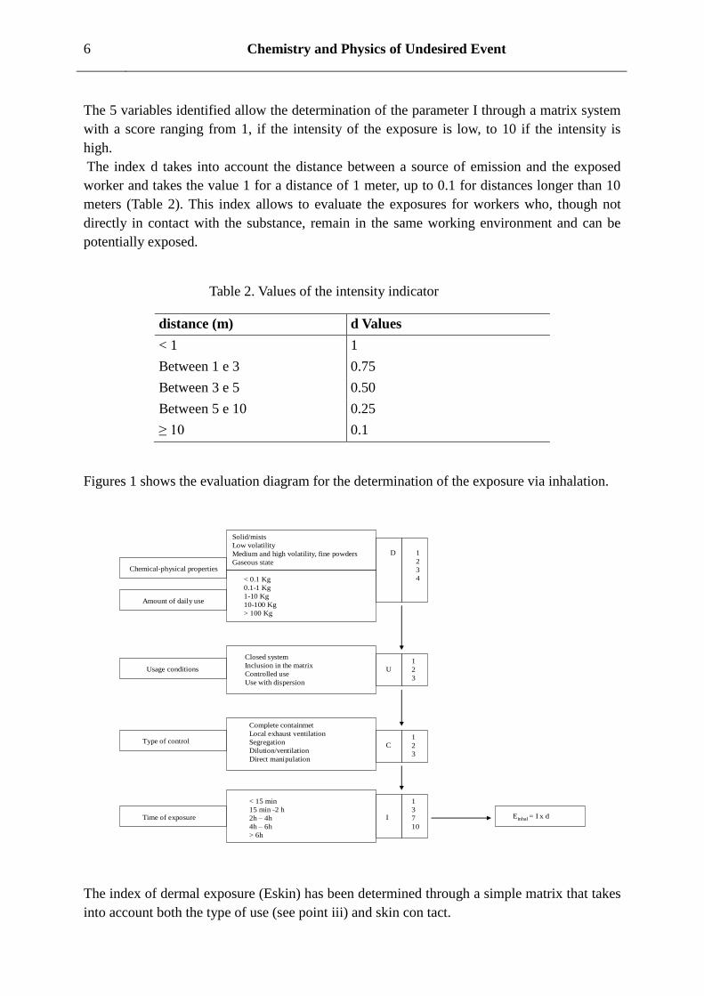
Figures 1 shows the evaluation diagram for the determination of the exposure via inhalation.
Chemical-physical properties
Solid/mists
Low volatility
Medium and high volatility, fine powders
Gaseous state
Amount of daily use
< 0.1 Kg
0.1-1 Kg
1-10 Kg
10-100 Kg
> 100 Kg
D 1
2
3
4
Usage conditions
Closed system
Inclusion in the matrix
Controlled use
Use with dispersion
U
1
2
3
Type of control
Complete containmet
Local exhaust ventilation
Segregation
Dilution/ventilation
Direct manipulation
C
1
2
3
Time of exposure
< 15 min
15 min -2 h
2h – 4h
4h – 6h
> 6h
I
1
3
7
10
Einhal = I x d
The index of dermal exposure (Eskin) has been determined through a simple matrix that takes
into account both the type of use (see point iii) and skin con tact.
International Journal of Risk Theory, Vol 2(no.2), 2012 7
4 possible degrees of skin contact have been identified (in ascending order):
a. No contact.
b. Accidental contact: no more than one event per day. Due to occasional spillage or releases.
c. Discontinuous contact: from two to ten events per day because of the production process.
d. Extended contact: the number of events per day is higher than ten.
After granting the assumptions corresponding to the two above mentioned variables and by
the help of the matrix for assessing skin, it is possible to assign the value of Eskin.
Calculated the exposure indices Einhal and Eskin and knowing the factors P of the substance,
the model calculates R according to formula (1), considering the combined effects on the
health and safety of workers due to exposure to multiple hazardous chemicals. The model
A.r.chi.me.d.e. makes possible to highlight the cumulative effects on health through the
recognition of the action of different substances on the same target organ. In this way, even
small exposures of multiple substances may lead to a judgment of not inconsiderable risk to
health, if all act in an unfavourable way on the same target organ.
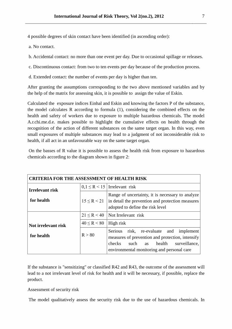
On the basses of R value it is possible to assess the health risk from exposure to hazardous
chemicals according to the diagram shown in figure 2:
CRITERIA FOR THE ASSESSMENT OF HEALTH RISK
Irrelevant risk
for health
0,1 ≤ R < 15 Irrelevant risk
15 ≤ R < 21
Range of uncertainty, it is necessary to analyze
in detail the prevention and protection measures
adopted to define the risk level
Not irrelevant risk
for health
21 ≤ R < 40 Not Irrelevant risk
40 ≤ R < 80 High risk
R > 80
Serious risk, re-evaluate and implement
measures of prevention and protection, intensify
checks such as health surveillance,
environmental monitoring and personal care
If the substance is "sensitizing" or classified R42 and R43, the outcome of the assessment will
lead to a not irrelevant level of risk for health and it will be necessary, if possible, replace the
product.
Assessment of security risk
The model qualitatively assess the security risk due to the use of hazardous chemicals. In
8 Chemistry and Physics of Undesired Event
fact, if you meet the following requirements, the level of security risk in the workplace will be
automatically low:
(i) in the workplace it is excluded the presence of:
1. hazardous concentrations of flammable substances;
2. chemically unstable substances;
3. other combustible oxidizing or similar materials,;
4. free flames, ignition sources or similar ;
5. easily volatile (boiling point below 65 ° C) and flammable substances.
(ii) the workplace is classified as having a low fire risk, according to current regulations.
In all cases where the security risk will be "not low", the proposed actions will be a more
thorough assessment of the risk or the replacement of the product.
4. ASSESSMENT OF CUMULATIVE EFFECTS
The model identifies substances that act on the same target organ, groups them and calculate
the health risk from cumulative effects, using in the algorithm:
- The Worsening group parameters;
- Amount as the sum of all the quantities of the substances;
- As a using way the worst condition;
- As distance the smallest from the source;
- Exposure time as the longest one;
- As danger index the highest.
Although the combined effects are not always additive, the most protective scenario for
workers should be considered, according to the principle of legislation for safety at work, and
considering also that toxicological data do not always exist for the various combinations of
substances, , the adopted method can then be used for security purposes.
5. METHODOLOGY
Three research laboratories of the University of Rome La Sapienza working in different
disciplinary areas of science have been monitored: they are two analytical chemistry
laboratories (laboratory ICP-MS and LC-MS lab) and a laboratory of organic synthesis. As
part of analytical chemistry, the two laboratories differ in the type of analytical investigations
undertaken and in the equipment used.
In the laboratory called ICP-MS methods for the analysis of inorganic substances in water
International Journal of Risk Theory, Vol 2(no.2), 2012 9
and particulate material in biological matrices, by means of mass spectrometry inductively
coupled plasma to (ICP-MS) have been developed and applied.
In the laboratory, referred to as LC-MS, methods for the characterization and analysis of
pollutants (pesticides, pharmaceuticals and emerging contaminants) in food, environmental
and biological matrices by liquid chromatography coupled to mass spectrometry (LC-MS )
have been developed and applied. In this laboratory there is also a section deputed to the
analysis of drugs of natural origin and synthetic.
In the laboratory of organic synthesis organic molecules biologically active, through a series
of reaction step have been synthesized; at the end of each step, the obtained results and the
reaction yields, for both synthetic intermediates and final products have been verified by
chromatographic analysis (GC-MS or LC-MS) spectrometry or infrared Fourier transform
(FTIR)
The process by which the risk assessment has been carried out is divided into six phases:
1. Preliminary fact-finding investigation;
2. verification and data collection in the laboratory using a checklist provided to individual
workers;
3. inspections at the workplace and observation of processing stages;
4. Acquisition of safety data sheets for substances and preparations;
5. data processing;
6. calculation and definition of risk.
The preliminary fact-finding investigation, conducted through meetings with researchers, it
was necessary for any clarification on the check list and for proper identification of
homogenous risk groups among workers. After analyzing all the activities carried out in the
laboratories, the hazardous properties of registered chemicals have been verified.
To calculate the inhalation and dermal index of exposure through the model Archi.me.de 3.0, ,
information on the daily amounts used for each chemical, the operation modes, exposure time
and the distance from the source have been derived from checklists completed by laboratory
workers.
For the chemical agents a "controlled, non-dispersive use" has been generally considered, as
the staff working in the laboratories normally has a highly specialized and professional
training.
Totally around 120 hazardous chemicals have been estimated, including 10 reaction
intermediates, synthesized in the laboratory of organic synthesis, to which, in the absence of
an official classification, it has been decided to assign risk phrases according to the molecular
10 Chemistry and Physics of Undesired Event
structure and of physical and chemical known properties.
In conducting the assessments, it has been necessary to adapt to a certain rigidity of the
algorithm, so the use of chemical agents has been rated as a daily, while in the practice of
laboratory activities, frequency of use were often minor, and not exactly quantifiable,
especially if referred to the individual operator. Moreover, the quantities actually in use were
generally much lower than the minimum defined by the algorithm of 0.1 Kg
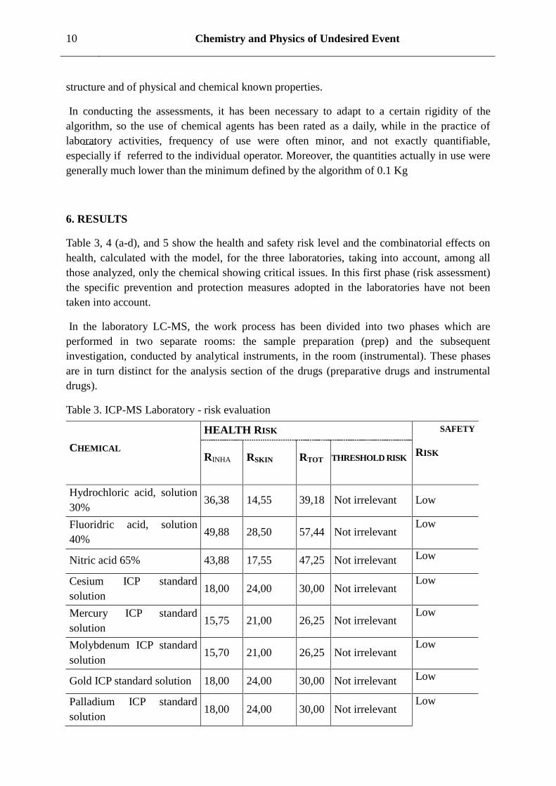
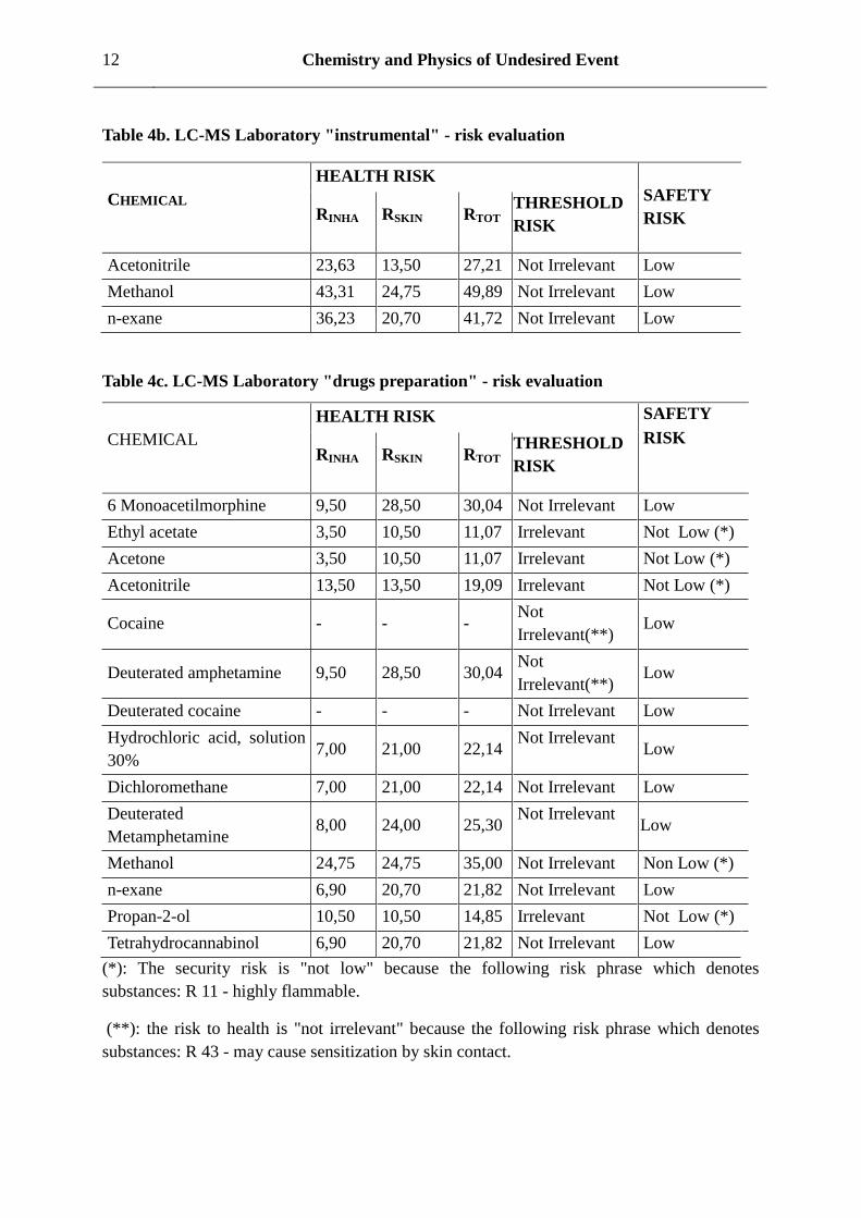
6. RESULTS
Table 3, 4 (a-d), and 5 show the health and safety risk level and the combinatorial effects on
health, calculated with the model, for the three laboratories, taking into account, among all
those analyzed, only the chemical showing critical issues. In this first phase (risk assessment)
the specific prevention and protection measures adopted in the laboratories have not been
taken into account.
In the laboratory LC-MS, the work process has been divided into two phases which are
performed in two separate rooms: the sample preparation (prep) and the subsequent
investigation, conducted by analytical instruments, in the room (instrumental). These phases
are in turn distinct for the analysis section of the drugs (preparative drugs and instrumental
drugs).
Table 3. ICP-MS Laboratory - risk evaluation
CHEMICAL
HEALTH RISK SAFETY
RISK
RINHA RSKIN RTOT THRESHOLD RISK
Hydrochloric acid, solution
30% 36,38 14,55 39,18 Not irrelevant Low
Fluoridric acid, solution
40% 49,88 28,50 57,44 Not irrelevant
Low
Nitric acid 65% 43,88 17,55 47,25 Not irrelevant Low
Cesium ICP standard
solution 18,00 24,00 30,00 Not irrelevant
Low
Mercury ICP standard
solution 15,75 21,00 26,25 Not irrelevant
Low
Molybdenum ICP standard
solution 15,70 21,00 26,25 Not irrelevant
Low
Gold ICP standard solution 18,00 24,00 30,00 Not irrelevant Low
Palladium ICP standard
solution 18,00 24,00 30,00 Not irrelevant
Low
International Journal of Risk Theory, Vol 2(no.2), 2012 11
CHEMICAL
HEALTH RISK SAFETY
RISK
RINHA RSKIN RTOT THRESHOLD RISK
Hydrogen peroxide 30% 13,16 5,85 14,40 Irrelevant Not Low(*)
Lead ICP standard solution 22,50 30,00 37,50 Not irrelevant Low
Potassium ICP standard
solution 7,43 23,10 24,26 Not irrelevant
Low
Selenium ICP standard
solution 16,31 21,75 27,19 Not irrelevant
Low
Silicon ICP standard
solution 18,00 24,00 30,00 Not Irrelevant
Low
Thallium ICP standard
solution 19,69 26,25 32,81 Not irrelevant
Low
Tellurium ICP standard
solution 18,00 24,00 30,00 Not Irrelevant
Low
Vanadium ICP standard
solution 19,13 25,50 31,88 Not Irrelevant
Low
(*): The security risk is "not low" because the following risk phrase that characterizes the
substance: R 5 - danger of explosion if heated
Table 4a. LC-MS Laboratory "Preparative" - risk evaluation
CHEMICAL
HEALTH RISK SAFETY
RISK RINHA RSKIN RTOT THRESHOLD
RISK
Acetone 24,50 10,50 26,66 Not Irrelevant Not Low(*)
Acetonitrile 13,50 13,50 19,09 Irrelevant Not Low(*)
Butyl hydroxy toluene 7,00 21,00 22,14 Not Irrelevant Low
Dichloromethane 21,00 21,00 29,70 Not Irrelevant Low
Methanol 8,25 8,25 11,67 Irrelevant Not Low (*)
n-exane 20,70 20,70 29,27 Not Irrelevant Low
Propan-2-ol 10,50 10,50 14,85 Irrelevant Not Low (*)
Trichloromethane 7,00 21,00 22,14 Not Irrelevant Low
(*)The security risk is "not low" because the following risk phrase that characterizes the
substances: R 11 – easily flammable
12 Chemistry and Physics of Undesired Event
Table 4b. LC-MS Laboratory "instrumental" - risk evaluation
CHEMICAL
HEALTH RISK SAFETY
RISK RINHA RSKIN RTOT THRESHOLD
RISK
Acetonitrile 23,63 13,50 27,21 Not Irrelevant Low
Methanol 43,31 24,75 49,89 Not Irrelevant Low
n-exane 36,23 20,70 41,72 Not Irrelevant Low
Table 4c. LC-MS Laboratory "drugs preparation" - risk evaluation
CHEMICAL
HEALTH RISK SAFETY
RISK RINHA RSKIN RTOT
THRESHOLD
RISK
6 Monoacetilmorphine 9,50 28,50 30,04 Not Irrelevant Low
Ethyl acetate 3,50 10,50 11,07 Irrelevant Not Low (*)
Acetone 3,50 10,50 11,07 Irrelevant Not Low (*)
Acetonitrile 13,50 13,50 19,09 Irrelevant Not Low (*)
Cocaine - - - Not
Irrelevant(**) Low
Deuterated amphetamine 9,50 28,50 30,04 Not
Irrelevant(**) Low
Deuterated cocaine - - - Not Irrelevant Low
Hydrochloric acid, solution
30% 7,00 21,00 22,14
Not Irrelevant Low
Dichloromethane 7,00 21,00 22,14 Not Irrelevant Low
Deuterated
Metamphetamine 8,00 24,00 25,30
Not Irrelevant Low
Methanol 24,75 24,75 35,00 Not Irrelevant Non Low (*)
n-exane 6,90 20,70 21,82 Not Irrelevant Low
Propan-2-ol 10,50 10,50 14,85 Irrelevant Not Low (*)
Tetrahydrocannabinol 6,90 20,70 21,82 Not Irrelevant Low
(*): The security risk is "not low" because the following risk phrase which denotes
substances: R 11 - highly flammable.
(**): the risk to health is "not irrelevant" because the following risk phrase which denotes
substances: R 43 - may cause sensitization by skin contact.
International Journal of Risk Theory, Vol 2(no.2), 2012 13
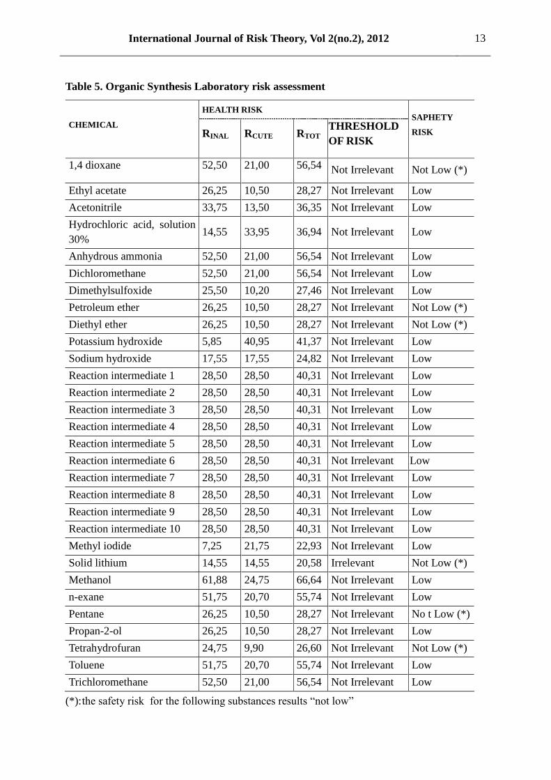
Table 5. Organic Synthesis Laboratory risk assessment
CHEMICAL
HEALTH RISK SAPHETY
RISK RINAL RCUTE RTOT THRESHOLD
OF RISK
1,4 dioxane 52,50 21,00 56,54 Not Irrelevant Not Low (*)
Ethyl acetate 26,25 10,50 28,27 Not Irrelevant Low
Acetonitrile 33,75 13,50 36,35 Not Irrelevant Low
Hydrochloric acid, solution
30% 14,55 33,95 36,94 Not Irrelevant Low
Anhydrous ammonia 52,50 21,00 56,54 Not Irrelevant Low
Dichloromethane 52,50 21,00 56,54 Not Irrelevant Low
Dimethylsulfoxide 25,50 10,20 27,46 Not Irrelevant Low
Petroleum ether 26,25 10,50 28,27 Not Irrelevant Not Low (*)
Diethyl ether 26,25 10,50 28,27 Not Irrelevant Not Low (*)
Potassium hydroxide 5,85 40,95 41,37 Not Irrelevant Low
Sodium hydroxide 17,55 17,55 24,82 Not Irrelevant Low
Reaction intermediate 1 28,50 28,50 40,31 Not Irrelevant Low
Reaction intermediate 2 28,50 28,50 40,31 Not Irrelevant Low
Reaction intermediate 3 28,50 28,50 40,31 Not Irrelevant Low
Reaction intermediate 4 28,50 28,50 40,31 Not Irrelevant Low
Reaction intermediate 5 28,50 28,50 40,31 Not Irrelevant Low
Reaction intermediate 6 28,50 28,50 40,31 Not Irrelevant Low
Reaction intermediate 7 28,50 28,50 40,31 Not Irrelevant Low
Reaction intermediate 8 28,50 28,50 40,31 Not Irrelevant Low
Reaction intermediate 9 28,50 28,50 40,31 Not Irrelevant Low
Reaction intermediate 10 28,50 28,50 40,31 Not Irrelevant Low
Methyl iodide 7,25 21,75 22,93 Not Irrelevant Low
Solid lithium 14,55 14,55 20,58 Irrelevant Not Low (*)
Methanol 61,88 24,75 66,64 Not Irrelevant Low
n-exane 51,75 20,70 55,74 Not Irrelevant Low
Pentane 26,25 10,50 28,27 Not Irrelevant No t Low (*)
Propan-2-ol 26,25 10,50 28,27 Not Irrelevant Low
Tetrahydrofuran 24,75 9,90 26,60 Not Irrelevant Not Low (*)
Toluene 51,75 20,70 55,74 Not Irrelevant Low
Trichloromethane 52,50 21,00 56,54 Not Irrelevant Low
(*): the safety risk for the following substances results “not low”
14 Chemistry and Physics of Undesired Event
- 1,4 dioxane (R 19)
- Petroleum ether (R 12)
- (Diethyl ether R 12 - R 19)
- Solid lithium (R 14/15)
- Pentane (R 12)
-Tetrahydrofuran (R 19)
For the proper management of chemical risk, for the only cases in which the index of potential
risk was not irrelevant to the health and not low to security, such measures have been
adopted:
- Use of adequate equipment and materials;
- Appropriate organizational and collective protection measures at source;
- Individual protection measures including personal protective equipment;
As measures of collective protection the use of fume hoods, has been provided, besides in
each laboratory there were systems for emergency eyewash and fire suppression systems.
Operators, already subject to health surveillance and receiving training in information and
formation, have been provided with personal protective equipment such as:
- Latex gloves, protection class 1 (breakthrough time> 10 min);
- Nitrile gloves, protective risk category III;
- Earpiece eye protection to stem.
Taking into account the specific adopted measures of prevention and protection, the new
levels of health risk have been determined in order to determine whether, as implemented in
the laboratories, it was sufficient to keep the risks to acceptable levels and content (
management of residual risk) .
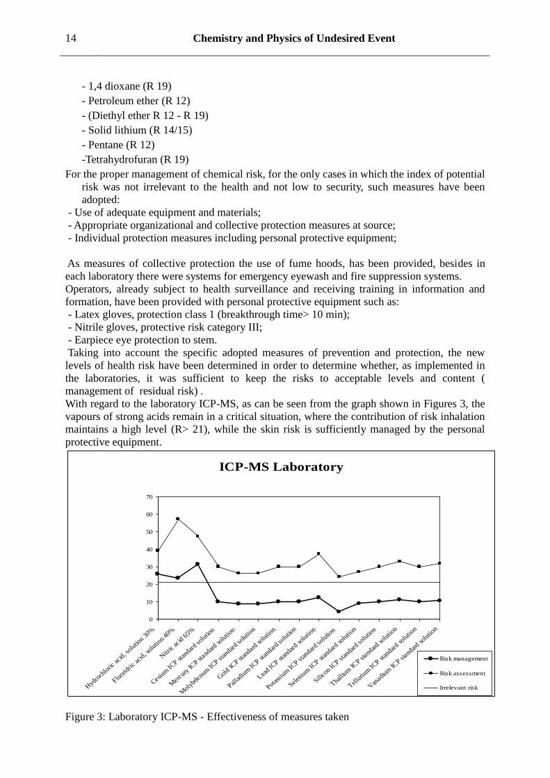
With regard to the laboratory ICP-MS, as can be seen from the graph shown in Figures 3, the
vapours of strong acids remain in a critical situation, where the contribution of risk inhalation
maintains a high level (R> 21), while the skin risk is sufficiently managed by the personal
protective equipment.
ICP-MS Laboratory
0
10
20
30
40
50
60
70
Hyd
roch
loric
acid
, sol
utio
n 30
%
Fluor
idric
aci
d, so
lutio
n 40
%
Nitr
ic ac
id 6
5%
Cesiu
m IC
P stan
dard
solu
tion
Mer
cury
ICP st
anda
rd so
lutio
n
Mol
ybde
num
ICP st
anda
rd so
lutio
n
Gol
d IC
P sta
ndar
d so
lutio
n
Palla
dium
ICP st
anda
rd so
lutio
n
Lead
ICP st
anda
rd so
lutio
n
Potas
sium
ICP st
anda
rd so
lutio
n
Selen
ium
ICP st
anda
rd so
lutio
n
Silico
n IC
P stan
dard
solu
tion
Thalli
um IC
P stan
dard
solu
tion
Tellu
rium
ICP st
anda
rd so
lutio
n
Van
adiu
m IC
P stan
dard
solu
tion
Risk management
Risk assessment
Irrelevant risk
Figure 3: Laboratory ICP-MS - Effectiveness of measures taken
International Journal of Risk Theory, Vol 2(no.2), 2012 15
With regard to the laboratory LC-MS, the new levels of health risk, show an acceptable
situation, except for the organic solvents used in the instrumental section and the presence of
sensitizers (cocaine and cocaine deuterated) in the section drugs. The data relating to solvents
are reported in Tables 6a-b.
Table 6a. Laboratory LC-MS “instrumental” –residual risk management
CHEMICAL
HEALTH RISK
RINHAL Rskin RTOT RISK
MANAGEMENT
acetonitrile 23,63 4,50 24,05 insufficient measures
methanol 43,31 8,25 44,09 insufficient measures
n- hexane 36,23 6,90 36,88 insufficient measures
Table 6b: Laboratory LC-MS “instrumental drugs” – residual risk management
CHEMICAL
HEALTH RISK
RINHAL RSKIN RTOT RISK
MANAGEMENT
acetonitrile 23,63 4,50 24,05 insufficient measures
methanol 43,31 8,25 44,09 insufficient measures
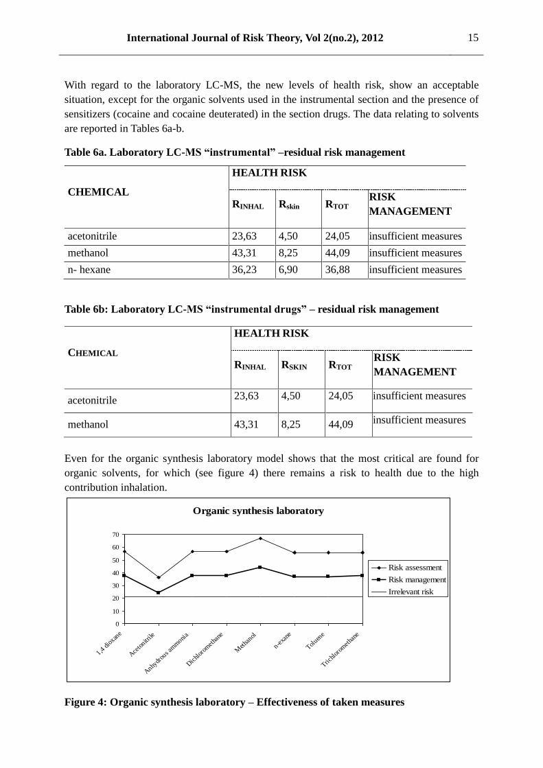
Even for the organic synthesis laboratory model shows that the most critical are found for
organic solvents, for which (see figure 4) there remains a risk to health due to the high
contribution inhalation.
Organic synthesis laboratory
0
10
20
30
40
50
60
70
1,4 d
ioxan
e
Ace
tonitr
ile
Anhy
drou
s am
moni
a
Dic
hlor
omet
hane
Met
hanol
n-exa
ne
Toluen
e
Trichl
orom
etha
ne
Risk assessment
Risk management
Irrelevant risk
Figure 4: Organic synthesis laboratory – Effectiveness of taken measures
16 Chemistry and Physics of Undesired Event
As can be seen from the results the greatest risk in the three laboratories is due to the
inhalation contribution, so it is necessary to strengthen the specific measures of prevention
and protection, with corrective actions such as adopting collection systems at source by local
exhaust ventilation, and, when possible , the change of the analytical methods for example by
decreasing the quantity of solvents used and the exposure times. Beyond this should be
assessed the feasibility of replacing the most hazardous substances with others of equal
efficiency but less problematic.
7. ASSESSMENT OF CUMULATIVE EFFECTS
This assessment is carried out automatically because the model uses all the data already
entered into the system to make individual assessments.
The calculation has been made with respect to the cumulative effects on target organs and the
information was derived from INAIL (Italian Workers' Compensation Authority) the table for
occupational diseases, with the exception of ototoxic effects derived from literature.
The cumulative risk on target organs has been calculated in both the absence of specific
measures (evaluation) and in the presence of these (management) in order to determine the
residual risk and the effectiveness of preventive and protective measures adopted.
The results obtained show that some organs are particularly fatigued by combinatorial effects,
even considering the measures put in place.
Specifically:
1. in the ICP-MS laboratory is the use of strong acids to create more problems, particularly
hydrofluoric acid, for which we observe a significant risk concerning the following
organs: respiratory tract, skin, eye and ocular annexes , the lymphatic system disorders ,
musculoskeletal and connective tissue.
2. in the LC-MS and organic synthesis laboratories, the contexts, in which the risk is not
negligible, mainly involves organic solvents, therefore the target organs of the cumulative
effects are: respiratory tract , skin, eye and ocular annexes, ear, central and peripheral
nervous system , liver and biliary tract.
The assessment of cumulative effects integrates the assessment of health risk and is useful to
the responsible physician for determining the health protocol.
8. CONCLUSIONS
The model A.r.chi.me.d.e. is simple, easy to apply and require a limited number of inputs.
However, we highlight some critical points that may be object of appropriate assessment to
adapt the algorithm to the examined context. The first consideration is on the unit measure,
Kg, the amount used by the algorithm, which is too high when put in relation to the amounts
International Journal of Risk Theory, Vol 2(no.2), 2012 17
used in research laboratories, where the weight used order is of grams or less.
The second consideration concern the intervals of exposure which are too wide and do not
allow to discriminate between phases having, for example, an exposure time of 16 minutes by
phases of 2 hours. On the basis of these considerations it can be seen as the score related to
the phrase R is preponderant in the calculation of P, without any attenuation for small amounts
and short times of exposure. The third critical point is that the frequencies of use are not
adequately considered and in this sector would be suitable to identify more precise
mechanisms linking the exposure times to the frequencies with which the work phases are
repeated throughout the day.
In conclusion it can be said that in chemical risk assessment for the research, the use of the
model Archi.me.de is a valid help to identify those situations where the risk is definitely
"irrelevant", and this is particularly useful when environmental monitoring is not possible,
but it should be improved, where critical issues were identified, for a better application it at
the university level.
REFERENCES
[1] European Commission, Regulation (EC) No 1907/2006 of the European Parliament and
of the Council of 18 December 2006 concerning the Registration, Evaluation,
Authorisation and Restriction of Chemicals (REACH), establishing a European
Chemicals Agency, amending Directive 1999/45/EC and repealing Council Regulation
(EEC) No 793/93 and Commission Regulation (EC) No 1488/94 as well as Council
Directive 76/769/EEC and Commission Directives 91/155/EEC, 93/67/EEC, 93/105/EC
and 2000/21/EC, Off. J. Eur. Commun L396; 1.
[2] European Commission, Regulation (EC) No 1272/2008 of the European Parliament and
of the Council of 16 December 2008 on classification, labelling and packaging of
substances and mixtures, amending and repealing Directives 67/548/EEC and
1999/45/EC, and amending Regulation (EC) No 1907/2006, Off. J. Eur. Commun L353.
[3] AA.VV. “La valutazione del rischio chimico nei laboratori chimici di ricerca pura e
applicata” Atti del Convegno: Esperienze del Servizio Prevenzione e Sicurezza Ambienti
di Lavoro della ASL RM, 2008. pp. 9-35.
[4] E. Strafella, M. Bracci, R. Calisti, M. Governa, L. Santarelli, LaboRisCh: un algoritmo
per la valutazione dei rischi per la salute da agenti chimici nei laboratori di ricerca e
negli ambienti di lavoro affini, Medicina del Lavoro, 99, 3, 2008, p.199-211.
[5] D.Lgs. n. 81 del 9 aprile 2008 “Attuazione dell'articolo 1 della legge 3 agosto 2007, n.
123, in materia di tutela della salute e della sicurezza nei luoghi di lavoro”, Gazzetta
Ufficiale n. 101 del 30 aprile 2008 - S.O. n. 108.
[6] European Commission, Council Directive 98/24/EC on the protection of the health and
safety of workers from the risks related to chemical agents at works, Off. J. Eur.
Commun. , L131; p.11-23.
18 Chemistry and Physics of Undesired Event
[7] Council Directive 98/24/EC of 7 April 1998 on the protection of the health and safety of
workers from the risks related to chemical agents at work. Off. J. Eur. Commun L131.
[8] R. Vincent, F. Bonthoux, G. Mallet, J.F. Iparraguirre, S. Rio, Methodologie d’evalutation
simplifiée du risque chimique : un outil d’aide à la decision, INRS – Hygiène et sécurité
du travail – Cathiers de notes documentaires, 3° trimestre 2005.
[9] Federal Institue for Occupational Safety and Health (BauA), Easy to use workplace
control scheme for hazardous substances, http://www.baua.de.
[10] H. Heussen, Stoffenmanager 4.0 – Exposure Modelling for Chemical safety Assessment,
http://www.stoffenmanager.nl.
[11] TURI Toxic Use Reduction Institute, Pollution Prevention Options Assessment System
(P2OASys), http://www.turi.org.
[12] Tuscany Region, Emilia-Romagna Region, Lombardia Region, Modello di Valutazione
del Rischio da agenti chimici pericolosi per la Salute ad uso delle piccole e medie
imprese (MoVaRisCH), aggiornamento ottobre 2008.
[13] European Commission Joint Research Centre, http://www.ecb.jrc.ec.europa.eu/
[14] ECETOC Target Risk Assessment, http://www.ecetoc.org/tra.
[15] J. Tickner, J. Friar, K.S. Creerly, J.W. Cherrie, D.E. Pryde, J. Kingston, The development
of the EASE model, Ann. occup. Hyg., 99, 2, 2005, pp.103-110.
[16] K.S. Creerly, J. Tickner, A,J. Soutar, G.W.Hughson, D.E. Pryde, N.D. Warren, R. Rae, C.
Money, A. Phillips, J.W. Cherrie, Evaluation and Further Development of EASE Model
2.0, Ann. occup. Hyg., 99, 2, 2005, pp.135-145.
[17] Council Directive of 27 June 1967 on the approximation of laws, regulations and
administrative provisions relating to the classification, packaging and labelling of
dangerous substances (67/548/EEC), Off. J. Eur. Commun., 196/1.
[18] Directive 1999/45/EC of the European Parliament and of the Council of 31 May 1999
concerning the approximation of the laws, regulations and administrative provisions of
the Member States relating to the classification, packaging and labelling of dangerous
preparation, Off. J. Eur. Commu.
International Journal of Risk Theory, Vol 2(no.2), 2012 19
MATHEMATICAL MODELS OF DECISION-MAKING IN COUNSELING
A. Maturo1, E. Sciarra
1, A. Ventre
2
1Department of Social Sciences, University of Chieti-Pescara 2Department of Culture of the Project and Benecon Center, Second University of Napoli
[email protected]; [email protected]; [email protected]
ABSTRACT
Some methodologies for practicing counseling are deepen in. The aim is in helping a
person to assume his/her autonomous decisions and then rational actions, coherent with
own identity and objectives. Moreover a mathematical formalization of the counseling
procedures is considered as a dynamical decision making problem, where the
awareness of alternatives and objectives and their evaluations are maieutically induced
by the Counselor. Finally it is shown that fuzzy reasoning can give a useful help to the
task of the Counselor, because of its flexibility and closeness to human reasoning.
KEYWORDS
Counseling, Multiobjective Decision Making, Fuzzy Reasoning, Uncertainty.
1. INTRODUCTION
In Sociology, there are many well-established methodologies for practicing counseling [2],
[5], [17], [18], [19], [20], [21], [25], [26]; on the other side in Mathematics and in Operational
Research there are many patterns of Decision Making [6], [7], [9], [11], [13], [16], [22] in
condition of certainty, randomness uncertainty [3], [4], [6], and semantic uncertainty [10],
[12], [29], [30]. The aim of our paper is to establish links among these theories and to look for
what possible help to practicing counseling can arise by suitable formalizations of problems in
terms of Decision Making theory.
The idea is that a cooperation among experts of different fields can give new points of view to
face problems of persons having unease. In particular the mathematical procedures utilized to
solve Decision Making problems can be very useful for the Counselor task of showing to the
Client the degree of coherence between his/her objectives and his/her actions and behaviors.
An important role is played by the de Finetti subjective probability [3], [4], [6]. Precisely, the
coherence between objectives and actions is obtained with a thought-out assessment of
probabilities to nature states and a rational aggregation of the issues associated to every
alternative. Moreover this prevents a too pessimistic or a too optimistic behavior, that are
consequences of not realistic evaluations of the possibility of occurrence of events.
Fuzzy reasoning and fuzzy algebra [1], [8], [14], [15], [24], [27], [28], [29], [30] can also give
a good contribution in the counseling procedure. Fuzzy reasoning permits a quantification and
a treatment of the semantic uncertainty and can help the Client to avoid extreme positions, and
to consider and mediate negative and positive aspects of every situation. Fuzzy algebra [8],

20 Economic and Financial Risk
[28], [29], [30] permits to consider the uncertainty in all the counseling processes, and
manage gradual modifications of the opinions of the Client induced by the maieutical activity
of the Counselor.
2. SOME MAIN FEATURES OF COUNSELING
Any counseling intervention pursues a general aim of development of competences and
resources, needed to confront and solve actual problems that a person may meet in the his/her
own path of life [2], [17], [18], [19], [20], [21], [25], [26].
The intervention concerns the support for the person to develop, in complete autonomy, a
knowledge of self, his/her own objectives, tools, contexts, actions, strategies to be able to
learn, confront and change the problems of his/her own personal and social development,
problems that are perceived like criticalities to solve.
The Counselor, in his own practices, exercises an aid process that, in a maieutic way, eases, in
the person, to emerge competences and the development of resources in the criticalities of the
own path of life. The aim consists in helping the person in his/her choices to assume
autonomous decisions and useful and rational behaviors in order to act with effectiveness and
satisfaction in own contexts perceived as problematic and difficult, with the ultimate aim to
reach self-realization and the wellness of the development.
This aim is realized with different methodologies and practices. In this paper we illustrate the
main features of the humanistic approach elaborated by Carl Rogers [20], [21] and Robert
Carkhuff [2]. This model presents the following main features, that are fundamental in
practicing counseling.
The practice of counseling by Carl Rogers, called ―non directive counseling‖, is centered on
the person of the Client, in order that an autonomous and positive base force of the person
emerges and operates.
Following Rogers, the Counselor accepts in the client the humanistic and existential dignity of
a capable person, that can address him/her-self. The Counselor non directive role assists the
person to implementing attitudes of reliance, authenticity, unconditional acceptation in the
interpersonal communicative climate between the Counselor and the interlocutor.
The helping relation has its main aim at inducing decision making autonomy, sense of dignity
and self-esteem of the person, who can experiment with a suitable climate of self-
determination, assumption of responsibilities, promotion.
Non directive method is not, however, the counterpart of a professional neutrality of the
Counselor, but an experience of full acceptation in the direction of the Client, to whom the
Counselor practices an interesting and tolerant communication. This disposition favors the
reliance of the person to change and develop him/her self toward a life more full and
satisfactory, inducing in the Client the capability of self-management to recognize and get
over the unease.

International Journal of Risk Theory, Vol 2(no.2), 2012 21
The empathetic technique of the Counselor consists in the attempt to understand and perceive
how the client perceives and understands, to come into his/her perceptive field of meanings,
where the whole situational experience finds fulfillments to realize the problem how it is lived
by the Client, with just his/her words and subjective universe.
The non directive role of the Counselor presents an empathetic and non judging
communication, without prejudices, that does not proceed by analysis and clinical
classification of the problems, but respecting the complete initiative of the Client, toward the
representation of his/her problem in the itinerary of the interview. The basis is a continuous
encouragement from the Counselor to a spontaneous expression of the Client autonomy, with
the goal to help him to search for his/her true self. Getting over the unease, the true
transformation of the situation and personality toward him/her-self, the environment and the
others, is just a client's concern: the Counselor can only help him to recover the freedom to be
him/her-self.
The task of the Counselor is to take care that the interviewee recovers his/her own integrity by
means of the consistent perception of his/her self. The person has a conceptual representation
organized by the self, like a fluid, but coherent, dynamic system of attributes and relations that
the ego assigns to the me in relation to the others. This system is self-organizing in front of the
natural and social context [23]. When lived experiences in the context are harmonic and
congruent with the concept of self, the person reach his/her own integrity and wellness,
otherwise the person is fragmented in the unease.
The existential humanistic approach of the Counselor is developed by his dispositional
attitudes, that consist in following the threads of Client's discourse, in a helping relational
climate of warm reception, comprehension, listening, without pre-determined schemes.
However, an operational methodology is outlined, mainly among Rogers followers, e. g.
Robert Carkhuff [2], with verbal reformulation technique of the Counselor, that aims to
deepen implicit meanings of the interviewee language and behavior, that give consistency and
visibility to the inner attitudes of the person.
Rogers' non directive and dispositional approach and the indirectly regulated and operational
one by Carkhuff are integrated on a level of greater complexity. The non directive aid of the
Counselor intends to make the Client's lived experience emerges autonomously, to help him to
find integrity, wellness, and coherence of his/her self. The indirect guide of the Counselor
does not neglect to reorganize the perceptions, the attitudes, the capabilities of the person
under unease, to help him/her to explore his/her own lived experience of behaviors in front of
the context, discover the contradictions, and find again the consistency between objectives
and effective actions.
In this way of operating, Carkhuff and his continuators elaborate a helping model, addressed
to the interpersonal processes management skills of the helper towards the helpee. The
operational methods of the Counselor are the verbal re-formulation of Client's words to
deepen the meaning of them, and the capability to pay attention, answer, personalize, involve,
explore, understand, compare, communicate and analyze impressions and evaluations… The
22 Economic and Financial Risk
aim of such sequential phases of the help process is to lead the person to awake to self, to
have knowledge of his/her problem, to make autonomous decisions, to reorganize perceptions,
behaviors and relations towards environment and persons. A progressive modification model
is sketched with the aim to solve the problems of wellness in a self-regulating way.
3. A MATHEMATICAL MODELING FOR COUNSELING
Some mathematical models for Counseling can be built starting from the patterns of Decision
Making and Game theories.
The first task of the Counselor is to obtain that, in a given instant t of the counseling
procedure, the Client is aware of a set At of own alternatives or strategies and a set Ot of own
objectives and is persuaded to look for the strategies that are coherent with own objectives
and to follow one of these strategies, dropping out the incoherent alternatives.
The sets At and Ot can change in the counseling process. The Counselor can obtain,
maieutically, that the Client be conscious of other alternatives and objectives, realizes that
some alternatives before considered are not feasible, or some objectives that seemed
important in a moment of emotion, actually are not important for his/her, and so can be
deleted from the list of the objectives.
A second task of the Counselor is to facilitate the Client in founding the relations between
his/her own objectives and each of his/her possible behaviors, in a coherent and realistic
vision of his/her wishes, tools, constraints, and possibilities; then the Client is assisted in
elaborating his/her evaluation of the situation with consequent framework of expectations,
perspectives of the possible alternatives, i.e. to understand how actions are tied with his/her
wishes.
The Counselor, using Ars Maieutica, and establishing together with the interlocutor a relation
that allows to attune his/her techniques to the emotional framework and the cognitive
objectives of the Client, has to get that the client himself builds his/her answers and decides
the own proper social actions.
Of course, the formalization should be understood ―as needed‖ and anyway it should be a
light, an ideal target, a far reference point, that gives the Client the logic framework of his/her
thoughts, in order that he/she avoids dispersions, incoherencies between wishes and effects of
his/her actions. A complete clarification of the objectives or a complete knowledge of the
alternatives is neither possible, nor desirable; indeed, an excess of detail increases the
complexity and loses sight of main logical thread.
The help of decision theory, in the construction of the frame of the expectations consequent to
each action, is important. The person to be oriented must be aware of what he/she gets, or the
frame of the possible outcomes related with any alternative and each his/her objective.
Decision theory helps to collect these data in order that the subject be oriented toward the
actions that are more coherent with his/her wishes.
Decisions may develop in certainty conditions or randomly. In other words an action may give
International Journal of Risk Theory, Vol 2(no.2), 2012 23
rise to just one or several possible consequences. The Counselor must help the Client to find
out the possible consequences of his/her actions and set choice criteria neither too optimist,
nor too pessimist. To this aim, a crucial help is given by subjective probability, based on the
coherence of the opinions. In fact, subjective probability allows to assess a coherent
probability distribution to the outcomes of an action.
Let {a1, a2, …, am} be the set of alternatives, {s1, s2, …, sr} the set of nature states, i.e. a set of
events pairwise disjoint and such that their union is the certain event. In the classical Decision
Making problem formalization the existence of the utility matrix U = (uih) is assumed, where
uih is a real number that represents the utility for the Decision Maker if he choose the
alternative ai and the event sh happens.
The pessimistic point of view leads to assume as score of ai the minimum, respect to h, of the
numbers mih, the optimistic one considers the maximum of such numbers. In [4], [6] it is
proved that a coherent point of view leads to obtain the score of every ai in two steps. Firstly,
a subjective probability assessment {p1, p2, …, pr} to the set of events {s1, s2, …, sr} is given.
After, the score of ai is assumed to be equal to the prevision of ai, given by the formula
P(ai) = p1 ui1 + p2 ui2 + … + pr uir. (1)
In [10], [12] fuzzy extensions of formula (1) are considered, starting by two different points of
view.
Of course, in practicing counseling, the Counselor must obtain probabilities pj and utilities mij,
in a maieutical way, by the Client. The coherent synthesis of the opinions of the Client is the
prevision (1).
The rational behavior is considering as scores of objectives a coherent synthesis of elements
of information or opinions. Lindley [6] claims that, if the utility matrix U = (uih) is given, only
the prevision is a coherent synthesis. But, in general, it is very difficult to obtain the matrix U.
In general, the maximum result of the activity of the Counselor is to lead the Client to give a
classification of pairs (ai, sj), from the most preferable to the least desirable, i.e. a preorder
relation is obtained.
In order to obtain numerical scores a useful procedure is Saaty’s AHP [13], [22]. This process
is based on questions that the Counselor proposes to the Client, with the aim to get measures
of the pairwise comparisons of the desirability of a set of objects (the pairs (ai, sj) in our case).
If there are many objectives and O = {o1, o2, …, on} is the set of objectives, then for every
objective oj, there is a different utility matrix Uj = (uih
j) and then, for every alternative ai and
objective oj, the prevision of ai with respect to oj is the real number
Pj(ai) = p1 ui1
j + p2 ui2
j + … + pr uir
j. (2)
24 Economic and Financial Risk
An important task of the Counselor is to help the Client to be aware of own objectives. Of
course, every person has a very high number of objectives in her/his life, and from the ars
maieutica of the Counselor the most important objectives of the Client must emerge and only
they are to be considered in the mathematical Decision Making model.
Moreover, the set O = {o1, o2, …, on} of the relevant objectives of the model must be
classified by the Client. The ideal situation is that the Client finds a rational way to associate
to every objective oj a positive real number wj that measures the importance that the Client
attributes to the objective oj.
Also for the weights of the objectives a suitable procedure is given by the AHP of Saaty [13],
[22]. For every pair (oj1, oj2) of objectives, the Counselor, with a set of questions, does the
Client say what is the one preferred or that the objective are equally preferred. In the first case
the Counselor must obtain by the client an integer number belonging to the interval [2, 9] that
measures to what extent the most preferred objective is more important for the Client than the
last preferred.
From the responses obtained, with the AHP procedure, a vector w = (w1, w2, …, wn) of
weights of objectives is obtained, where wj is a positive real number expressing the
importance that the Client gives to the objective oj, and the following normalization condition
is satisfied:
w1 + w2 + … + wn = 1. (3)
Before to implement the mathematical procedure to obtain the vector w a verification of the
coherence of the responses is necessary. In particular the transitivity of the preferences must
be verified. On the contrary, the Counselor, with a patient procedure, must propose the
questions in a different form in order to avoid incoherence.
When the previsions Pj(ai) and the weigths wj are obtained, a rational measure of the
opportunity of the action ai by the Client is given by the following score
s(ai) = w1 P1(ai) + w2 P
2(ai) + … + wn P
n(ai). (4)
The greater is the number s(ai), the more agreeable is the action ai. We emphasize that this
conclusion is only a coherent consequence of the opinions of the Client and the assumption of
particular mathematical procedures (e.g., the consideration of formula of prevision or formula
(4) to aggregate information on weights and previsions).
Obtaining scores s(ai) is important mainly as an help to the Decision Making, without a claim
to be definitive and not modifiable preference measure of the opportunity of the Client
actions.
International Journal of Risk Theory, Vol 2(no.2), 2012 25
4. FUZZY REASONING FOR COUNSELING
Fuzzy reasoning and arithmetic may help. They permit a gradual procedure in the changes of
points of view, gradual and dynamical attribution of the degrees of importance to the
objectives, management of semantic and emotional uncertainty.
Furthermore, the consequences of an action cannot be, in general, defined in a sharp way;
rather it is opportune that the Client does not renounce to his/her doubts in favor of a choice
that is rash, premature and of doubtful effectiveness. From this point of view, fuzzy logic and
linguistic variables may be effective, in that they are expressed as imprecise numbers, but
plastic and gradually modifiable numbers as far as the opinions of the Client become more
clear.
The fuzzy extensions of the decision theory are able to gather the various elements and shows
a clear framework, in a language that is close to the human language, of the path that goes
from the awareness of the own proper expectations to the coherent action.
In particular, the utility matrix U = (uih) considered in the previous Sec. is replaced by a
matrix U* = (uih*) where every uih* is a fuzzy number that expresses a value of a linguistic
variable [29], [30]. Moreover, the probability assessment is replaced by an assessment of
fuzzy probabilities {p1*, p2*, …, pr*} to the set of events {s1, s2, …, sr}, where every ph* is a
fuzzy number with support contained in the interval [0, 1].
By considering the Zadeh’s extensions [28], [29], [30] of the usual addition and multiplication
to fuzzy numbers, or alternative fuzzy operations [8], for every alternative ai, we can
introduce the fuzzy prevision [10], [12] by means of the formula
P*(ai) = p1* ui1* + p2* ui2* + … + pr* uir*. (5)
If the importance of the objectives is expressed by values of a linguistic variable, then also the
weights of objectives are fuzzy numbers wj*, j = 1, 2, …, n. Then formula (4) is replaced by
the more general
s*(ai) = w1* P*1(ai) + w2* P*
2(ai) + … + wn* P*
n(ai), (6)
where the addition is the extension of the usual addition with the Zadeh extension principle
and the multiplication is an approximation of the Zadeh multiplication, built with the aim to
preserve the shape of the class of the considered fuzzy numbers [8].
Unlike numbers s(ai), in general the fuzzy numbers s*(ai) are not totally ordered. This can
appear a drawback by a mathematical point of view, but, on the contrary, it is an advantage in
the practice of the counseling, as the fuzzy number s*(ai) contains, in its core and in its
support, the history of the uncertainty of the opinions of the Client and then it is a more
realistic global representation and it is a measure of the opportunities of his/her choices, more
coherent with his/her opinions.
26 Economic and Financial Risk
5. CONCLUSIONS
From previous Secs. it seems natural the conclusion that an interaction between the maieutical
ability and capability to find strategies of the Counselor and the power of the mathematical
models for Decision Making can be very useful to solve unease problems e to show to the
Client a clear vision of the consequence of her/his possible actions.
The illusory certainties, obtained by questionable assumptions, must be replaced by controlled
uncertainties. The tools to take into account the uncertainties and control their consequences
in all the counseling procedures are the probabilistic and fuzzy reasoning. In particular, before
any action it is necessary to have some information about the facility of occurrence of nature
states and this leads to consider the de Finetti subjective probability. More in general, the
uncertainty on the assessments of these probabilities can be controlled by considering fuzzy
subjective probabilities expressed by fuzzy numbers.
The utility of an action with respect to an objective is often very doubtful. Such uncertainty
can be controlled by measuring the utilities with fuzzy numbers.
In the fuzzy ambit, the aggregation of utilities and subjective probabilities associated to every
possible action of the Client is made with the tools of the fuzzy algebra and the fuzzy
reasoning. They permit to obtain, as a final score of every action, a fuzzy number that
provides not only a measure of the validity of this action, but also contains a résumé of the
whole history of doubts and uncertainties on the process of evaluation.
A treatment of the aggregation of the previsions and the weights of objectives more
sophisticated than the one considered in the previous Sec. takes into account also the logical
relations among the objectives [12], [14], [15], [16]. A generalization of the utilities is
obtained by utilizing fuzzy measures decomposable with respect to a t-conorm [1], [24],
[27]. From such a viewpoint a fuzzy prevision can be defined, in which the addition is
replaced by the operation . Applications of these theories to Decision Making may be found
in [12], [14], [15], [16].
However, as a final result of the application of the mathematical model, the Client obtains a
vector of fuzzy (in particular crisp) numbers s* = (s*(a1), s*(a2), …, s*(am)), where s*(ai)
measures the advisability of the action ai, taking into account all the opinions and doubts
expressed by the Client and the end of the maieutic work of the Counselor.
The vector s* is an important reference point for Counselor and Client, a basis for
understanding the consequences of their future activities, interactions, strategies and actions.
International Journal of Risk Theory, Vol 2(no.2), 2012 27
REFERENCES
[1] Banon G.: Distinction between several subsets of fuzzy measures. Int. J. Fuzzy Sets and
Systems 5, 291--305 (1981)
[2] Carkhuff R.R.: The Art of Helping. Amherst. MA: HRD Press (1972)
[3] Coletti G., Scozzafava R.: Probabilistic Logic in a Coherent Setting. Kluwer Academic
Publishers, Dordrecht (2002)
[4] de Finetti B.: Theory of Probability. J. Wiley, New York (1974)
[5] Di Fabio A.: Counseling. Dalla teoria all’applicazione. Firenze, Giunti. (1999)
[6] Lindley D.V.. Making Decisions. John Wiley & Sons, London (1985)
[7] March J.G.: A primer on Decision Making. How Decision Happen. The Free Press. New
York (1994)
[8] Maturo A.: Alternative Fuzzy Operations and Applications to Social Sciences.
International Journal of Intelligent Systems, Vol. 24, pp. 1243--1264 (2009)
[9] Maturo A, Ventre A.G.S.: Models for Consensus in Multiperson Decision Making. In:
NAFIPS 2008 Conference Proceedings. Regular Papers 50014. IEEE Press, New York.
(2008)
[10] Maturo A., Ventre A.G.S.: On Some Extensions of the de Finetti Coherent Prevision in a
Fuzzy Ambit. Journal of Basic Science 4, No. 1, 95--103 (2008)
[11] Maturo A, Ventre A.G.S.: Aggregation and consensus in multiobjective and multiperson
decision making. International Journal of Uncertainty, Fuzziness and Knowledge-Based
Systems, Vol. 17, No 4, 491--499 (2009)
[12] Maturo A, Ventre A.G.S.: Fuzzy Previsions and Applications to Social Sciences. In:
Kroupa T. and Vejnarová J. (eds.). Proceedings of the 8th Workshop on Uncertainty
Processing (Wupes’09) Liblice, Czech Rep. September 19-23, 2009, pp. 167--175 (2009)
[13] Maturo A, Ventre A.G.S.: An Application of the Analytic Hierarchy Process to Enhancing
Consensus in Multiagent Decision Making. In: ISAHP2009, Proceedings of the
International Symposium on the Analytic Hierarchy Process for Multicriteria Decision
Making, July 29- August 1, 2009, University of Pittsburg, Pittsburgh, Pennsylvania, paper
48, 1--12 (2009) [14] Maturo A., Squillante M., and Ventre A.G.S.: Consistency for assessments of uncertainty
evaluations in non-additive settings. In: Amenta, P., D'Ambra, L., Squillante, M., Ventre, A.G.S. (eds.) Metodi, modelli e tecnologie dell’informazione a supporto delle decisioni, pp. 75--88. Franco Angeli, Milano (2006)
[15] Maturo A., Squillante M., and Ventre A.G.S.: Consistency for nonadditive measures: analytical and algebraic methods. In: Reusch, B. (ed.) Computational Intelligence, Theory and Applications, pp. 29--40. Springer, Berlin (2006)
[16] Maturo A., Squillante M., and Ventre A.G.S.: Decision Making, Fuzzy Measures, and Hyperstructures, Advances and Applications in Statistical Sciences, to appear
[17] May R.: The art of Counseling. Human Horizons Series. Souvenir Press. New York (1989)
[18] Nanetti F.: Il Counseling: modelli a confronto. Pluralismo teorico e pratico. Quattroventi,
Urbino (2003)
[19] Perls F., Hefferline R.F., Goodman P.: Gestalt therapy. Julian Press, New York. (1951)
[20] Rogers C.R.: Client-Centered Therapy: Its Current Practice, Implications, and Theory.
Houghton Mifflin (1951)
[21] Rogers, C. R.: Counseling and psychotherapy, Rogers Press, Denton, Texas (2007)
[22] Saaty T.L.: The Analytic Hierarchy Process. McGraw-Hill, New York (1980)
[23] Sciarra E.: Paradigmi e metodi di ricerca sulla socializzazione autorganizzante. Edizioni
Scientifiche Sigraf, Pescara. Italy (2007)
[24] Sugeno M.: Theory of fuzzy integral and its applications, Ph. D. Thesis, Tokyo (1974)
[25] Thorensen C., Anton J.: Intensive Counseling, ―Focus on Guidance‖, 6, 1—11 (1973)

28 Economic and Financial Risk
[26] Tosi D.J., Leclair S.W., Peters H.J., Murphy M.A.: Theories and applications of
counseling. Charles Thomas publisher. Springfield (1987)
[27] Weber S.: Decomposable measures and integrals for Archimedean t-conorms. J. Math.
Anal. Appl. 101 (1), 114--138 (1984)
[28] Yager R.: A characterization of the extension principle. Fuzzy Sets Syst;18:205--217
(1986)
[29] Zadeh L.: The concept of a linguistic variable and its application to approximate
reasoning, Inf Sci 1975;8, Part I:199–249, Part 2: 301--357 (1975)
[30] Zadeh L.: The concept of a linguistic variable and its applications to approximate
reasoning, Part III. Inf Sci;9: 43--80 (1975)
International Journal of Risk Theory, Vol 2(no.2), 2012 29
A GAME THEORETIC APPROACH FOR A REINSURANCE MARKET
Manuela Ghica
Spiru Haret University, Faculty of Mathematics and Informatics, Bucharest
ABSTRACT
We give a survey for a reinsurance market. We present a game theoretic approach for some
important concepts useful in the analysis of reinsurance as the core, the bargaining set or the
Nash equillibrium. We propose some new results for a game model applied in the case of
reinsurance market and then we define and give some applications with exponental and power
utility functions for the market core, market core cover, stable sets of portfolios, the
Reasonable and the Weber sets for a reinsurance market.
KEYWORDS
reinsurance market, optimal allocations, core.
1. INTRODUCTION
The human desire for security and fighting against unpredictable future were first steps for
appearing ideas of insurance. At first, insurance means finding support in family, community
or guild and it has the origins in marine commerce. Even in Chistian era there were transport
covers but the oldest known contract with reinsurance characteristics was discovered much
later in 1370, in Genoa.
The reinsurance business has an important and vital role in country economies because it
represents a protection from the risks for the participants in the reinsurance market, i.e., for
the insurance companies. In a reinsurance market there is a transfer of risks to reinsurers for
reducing the fluctuations in the business performance of the insurance market, and, also, for
their capital costs.
"Reinsurance is a highly international industry with a limited number of large companies. In
2002, the total reinsurance premiums of the 40 largest reinsurance groups amounted to USD
138 601 200 000, whereof USD 58 544 000 000 stemmed from EU reinsurers. In EU,
Germany has a dominant position with companies as Munich Re, Hannover Re and Allianz
Re, Lloyd's is the largest UK writer of reinsurance, and SCOR together with Axa Re are the
largest French reinsurers"(Standard&Poor's, Global Reinsurance Highlights 2003 Edition,
London/New York, 2003). Today, Standard&Poor gives a list with almost 135 professional
reinsurers worldwide, as well as around 2000 direct insurers that also underwriting for the
insurance companies.
30 Economic and Financial Risk
The predecessor of the big group of professional reinsurance companies was the Cologne
Reinsurance Company, founded in Hamburg, in 1842, after a catastrophic fire which provoked
losses of 18 million marks. So, after marine insurance, the first big step in writing history of
reinsurance was insurance against fire hazards
The reinsurance market is the secondary market for insurance risks. The agents who are the
direct insurers rarely trade risks with each other. For this reason, they cede percent of their
initial risks to specialized professional reinsurers who have no primary business.
Reinsurance business is a prominent part of the non-life insurance market. From information
given by OECD it is known that only 10% of all insurance premiums are insured and, more,
18% of non-life insurance premiums are insured, compared to 3% for life insurance premium
average. The main roles of reinsurance for the cedant, i.e., the direct insurer who cede a some
percent of his risks, can be summarized as follows:
reduction of technical risks;
permanent transfer of technical risks to the reinsurer;
increase of homogeneity of insurance portfolio;
reduction of volatility of technical results;
substitute for capital/own funds;
supply of funds for financing purposes;
supply of service provision.
We can easily see that the underwriting policy of the cedant to a large extant is determined by
its reinsurance policy. The financial strength of a cedant and its ability to fulfill obligations
arising from insurance contracts vis-a-vis the policyholders depends clearly on the security of
the cedant's reinsurance arrangements.
In spite of its powerful connection to direct insurance industry, there are some characteristic of
reinsurance that may be important to underline before going into more specific issues. We will
describe some particularities of reinsurance:
there is no direct contractual relationship between the originally insured and the reinsurer,
and the policyholders have no priority to the assets of the reinsurer to cover their claims;
reinsurance is a business activity between professional parties;
reinsurers largely depend on information from the direct insurers to establish claims
reserves. There are furthermore significant delays in receiving claims information;
for reinsurers the volume of nonlife operations significantly exceeds that of life
operations;
International Journal of Risk Theory, Vol 2(no.2), 2012 31
reinsurance business has higher degrees of diversity in respect of geography and
combinations of insured lines than direct insurance business;
reinsurers have significant catastrophe exposure, and special retrocession and pooling
techniques to cope with those.
2. SOME MAIN DIRECTIONS
The theoretical study of insurance and reinsurance market equilibrium has been carry out
under a variety of models. The one of the first results were given by Arrow [10] and Debreu
[29] who used contigent space to study economic equilibrium in a simple risk exchange model
with two risk averse parties. In this way, using the contingent space, these authors were able to
extend certain fundamental results of economic equilibrium from an exchange of goods to an
exchange of risks. They proved that competitive equilibrium exists and that both the first and
the second social welfare theorems hold in an economy with uncertainty. Specifically, they
showed that competitive equilibrium is Pareto optimal, and every Pareto optimal solution can
be supported by a competitive equilibrium through the redistribution of endowments.
By using contingent space the economists can analyze uncertainty, it is far removed from
reality of most insurance markets. In 1962 Borch presented a risk exchange model of the
reinsurance market and he argued that this kind of market should contain only one price,
rather than the multiplicity of prices associated with all possible states in contingent space.
Because the Borch's model was over-specified, in 1971 Kihlstom and Pauly [38] showed the
form of this kind of risk loading was not consisting with the assumption's Borch that the
parties in the risk exchange had quadratic utility functions. Kihlstom and Pauly demonstrated
that the single price of insurance is correlated with the prices of contingent claims, and that
the competitive equilibrium of a risk exchange in price/quantity space is consistent with
competitive equilibrium of a risk exchange in contigent space.
Subsequently, Arrow [11] noted the risk transfer - as opposed to risk exchange- model
recognizes the reality that the parties in most traditional insurance markets are either buyers
and sellers, and not suitable both to cede and to assume risk as in a risk exchange.
The reinsurance problem appears at first sight to be a problem which can be analyzed in terms
of classical economic theory, if the objectives of the companies have been formulated in an
operational manner by the help of Bernoulli's utility concept: it must not be maximized the
expected gain, but the expected utility of the gain. "The ideas of Bernoulli reappeared in
insurance literature only when the game theory of von Neumann and Morgenstein had made
utility fashionable, and demonstrated that this concept must occupy a central position in any
theory of decisions under risks and uncertainty"[24]. However, closer investigations show that
the economic theory is only relevant part of the way. Then the problem becomes a problem of
cooperation between parties who have conflicting interests, and who are free to form and
break any coalitions which may serve their particular interests. Classical economic theory is
powerless when it comes to analyze such problems. The only theory which at present seems to
32 Economic and Financial Risk
hold some promise of being able to sort out and explain this apparently chaotic situation, is
Games Theory.
In insurance mathematics, beginning perhaps with the works of Borch [17, 18, 21, 22], later,
Baton and Lemaire [15, 16] applied the Nash bargaining framework of cooperative game
theory to the analysis of a reinsurance market. Kihlstrom and Roth showed in a similar
analysis of a risk transfer between one insured and one insurer [39]. Game theoretic ideas
have been used in the context of reinsurance by many authors but the recent papers belong to
Aase [3, 8].
To succeed the implementation of the real cases from a reinsurance market in a theoretical
structure who belong to game theory some elements hold:
Participants have some benefits to share ( political power, savings, or money);
The opportunity to divide results have to results from cooperation of all participants or a
sub-group of participants;
Individuals are free to engage in negotiations, bargaining, coalition formation;
Participants have conflicting objectives; each wants to secure the largest part of the
benefits for himself.
Cooperative game theory studies those situations where participants' objectives are partially
cooperative and partially conflicting. The biggest interest of the participants is to cooperate
because in this way they can achieve the greatest possible total benefits. When it comes to
sharing the benefits of cooperation, however, individuals have conflicting goals. Such cases
are usually modeled as n - person cooperative games in characteristic function form.
3. REINSURANCE MARKET. OPTIMAL PORTFOLIOS
The economists propose two theoretical patterns to analyze reinsurance. K. Borch, in 1962,
was the first one, who proposed a new method [21], for studying the reinsurance market,
based on optimal risk sharing among risk-averse agents.
Later, in 1990, the second pattern to investigate a reinsurance market was taken from
corporate hedging theory. This approach is based on the decision of a insurer to get
reinsurance looks like the decision of any nonfinancial business to acquire reinsurance.
It was revealed that both approaches keep unexplained problems and, also, pass up the dual
approach of the theory of reinsurance. The last observation was attacked in them study by
Garven and Lamm-Tennant [32], when the reinsurance is both a risk management and a
financing decision.
The optimal allocation problem, based on Borch theory, is the problem of allocation a risk in a
optimal way to n players supplied with risk measures. K. Borch used in his theoretical
approach an utility function Pareto to characterize optimal exchanges but without unique
International Journal of Risk Theory, Vol 2(no.2), 2012 33
solution [17, 18, 21]. This kind of solution may carry on substantial fixed sidepoints. These
results give to many authors the idea of game theoretic approach, or additional, concepts like
fairness. With this new point of view, game theory way, they reached to some specific
elements in the set of Pareto optimal rules [18, 30, 13, 40, 15, 27, 3].
The reinsurance market can be analyzed as a game. The players seen as traders enter in the
game with an initial allocation of risks, transform these goods and they go out with final
allocation with a higher utility.
This section presents a short overview on reinsurance market and it is based on results
established by Borch [17, 18, 23], Baton and Lemaire [15, 16], Aase [2, 3, 4, 6, 8].
Karl Henrik Borch is considered as the founding father of modern insurance economics. He is,
in fact, more originally an actuary then in economics and finance. Since 1960 till 1974, he
published the study of traditional actuarial problems as the theory of risk, optimal reinsurance
or optimal insurance asset allocation. In his study he used expected utility analysis and the
theory of games. Utility theory it is involved for the first time by Borch [20] for solving
actuarial problems. The theory about Pareto-optimal risk exchanges and general economic
equilibrium under uncertainty was developed for reinsurance markets but, later, it is shown
that it could be applied also for capital markets. In this research it is proof the Borch's theorem
on optimal risk exchange. The theorem shows that the exchange of risks is Pareto optimal if
and only if a pool contains all risks, and each agent takes a part in this pool. All risk exchange
model was developed during many research years [17, 19, 21, 25]. Also, there are some
important textbooks which it can be found self-contained presentations of the Borch's model
as Borch [25], B ..u hlmann [26], Gerber [33], among many others.
With his research in study of insurance and reinsurance markets K. Borch create a connection
between actuarial science and the economic under uncertainty.
We present in the following some important theorems which belong to the basic model, in its
original version:
Consider a set N C1 , . . . ,Cn of n agents (policyholders, insurance companies,
reinsurers,...) willing to improve their level of security through a risk exchange treaty. C j has
an initial wealth Rj and is subject to a risk, characterized by its distribution function F jx j
. Assume Cj evaluates his situation by means of utility function ujx, such that
ujx 0 and uj
x 0 for all x . The expected utility of C j 's initial situation
Rj,Fjx j is
U jx j U jRj,F jx j
0
ujRj x j dFjx j.
The members of the set of agents will then try to increase their utilities by concluding a treaty,
y y1x1 , . . . ,xn , . . . ,ynx1 , . . . ,xn
34 Economic and Financial Risk
where yjx1 , . . . ,xn yjx is the sum C j has to pay if the claims for the different agents
respectively amount to x1 , . . . ,xn .
Since all claims have to be indemnified, the treaty has to satisfy the following admissibility
condition.
Condition
i1
n
yjx i1
n
x j z *
where z denotes the total amount of all claims.
After the risk exchange, the expected utility of agent C j becomes
U jy N
ujRj yjxdFNx
where N is the positive orthant of En , and FNx is the n dimensional distribution
function of the claims x x1 , . . . ,xn . Thus, U j was extended from individual x j to
vector y1 , . . . ,yn .
A treaty y is obviously preferred to y if U jy U jy, for all j, with at least one
strict inequality. y is then said to be dominated by y. The set of undominated treaties is
called the efficient set or the pareto-optimal set.
Condition A treaty y is Pareto-optimal if there is no y such that U jy U jy for all
j, with at least one strict inequality.
Theorem A treaty y is Pareto-optimal if and only if there exists n non-negative constants
k1 , . . . ,kn , such that, almost surely,
k jujRj yjx k1u1
R1 y1x j 1, . . . ,n **
Note that F jx j does not appear in equation (**). Hence, the shape of the Pareto-optimal
treaties does not depend on the claim amounts distribution functions.
Later, du Mouchel proofs that there exists at least one Pareto-optimal treaty if there are mild
technical conditions [31].
Theorem If the k j can be chosen in such a way that the domains of the functions k jujx
have a nonvoid intersection, then there exists a Pareto-optimal treaty.
International Journal of Risk Theory, Vol 2(no.2), 2012 35
Theorem If the yjx are differentiable, a Pareto-optimal treaty depends only on the
individual claim amounts x j through their sum z .
The Borch's risk exchange model of reinsurance, researched as a n person cooperative
game, was studied by Lemaire [40, 41, 42], Lemaire and Baton [15]. In them studies they
approached game theoretic characteristics as the Pareto-optimal payoffs, core, bargaining set,
value of the game. Also, Lemaire found some applications of the famous Borch's theorem
[43].
Lemaire completed the existence theorem with a new result:
Theorem For each set K of constants k1 , . . . ,kn satisfying the assumption of the Borch's
existence theorem, there exists one, and only one, the Pareto-optimal treaty.
It was shown by Lemaire that the risk exchange model could be seen as a n -person
cooperative game without transferable utilities [43]. From this point of view was natural to
characterize the set of Pareto optimal treaties using ideas from game theory. Indeed, it was
obvious to introduce the condition about individual rationality.
Condition
U jy U jx j, j 1, . . . ,n.
When we have exponential utilities and independent claim amounts distribution Lemaire by
helping the Individual Rationality Condition reduce the upon bounds on the monetary
payments [42]:
yj0 P j
j P jN, j 1, . . . ,n.
The last two conditions don't exclude the phenomenon like some agents could win more if
they go out and constitute a subcoalition. This phenomenon is characterized in game theory as
a core of a game. Let define firstly this notion.
Let N be a set with n players. Let S N be a subcoalition, and vS be the set of Pareto-
optimal treaties for S ; y is said to dominate y with respect to coalition S if
1) U jy U jy , j S
2) S can impose y : y vS
or y is said to dominate y with respect to S . Hence, the core is said to be the set of all
the nondominated treaties. With this approach the Individual Rationality Condition could be
replaced with a stronger one, Collective Rationality Condition, which implies both last two
36 Economic and Financial Risk
conditions.
Condition No coalition has interest in leaving the pool.
Baton and Lemaire studied the case of risk exchange market for exponential utility with the
following result [15]:
Theorem y belongs to the core of the pool if and only if
yjx1 , . . . ,xn qjz yj0
with
jS
yj0 jS
P jS P j
N S N
defining Pj 0.
According to Baton and Lemaire [15]: "the main disadvantage of the core is that there exists
large classes of games for which it is empty. Fortunately, the next theorem shows the core of
the risk exchange market always exists."
Theorem The core of the market is non-void.
Not only the concept about core was studied in a risk exchange market, but, game theory has
produced other important solutions like:
1) Bargaining set
This is a solution concept introduced by Aumann and Mascheler [13], but the most used
definition belong to Davis and Mascheler [28]. If the core solution consists of all
allocations such that no coalition can propose an alternative set of trades, perception about
bargaining set that it limits the ability of coalitions to refrain a proposed payoff allocation
because of the apprehension that a second coalition can cause another counter object (set
of trades).
2) Kernel
The kernel solution was introduced by Davis and Mascheler and is defined in the same
way as the bargaining set relative to a partition Q of N . The perception about this
concept is that if two agents i , j belong to the same partition, then the higher excess
that i can realize in a coalition without j should be the same as the same excess like j
in the same situation with i .
3) Nucleolus
International Journal of Risk Theory, Vol 2(no.2), 2012 37
This solution concept was introduced by Schmeidler [48]. It is an imputation which is
reached minimizing, firstly, the largest excess among all coalitions, and so on till the end,
when remaining only one, so the kernel is unique imputation. If the core is non-empty
then the nucleolus belong to the core, also, it is always in kernel and, since the kernel is
contained in bargaining set.
These concepts were studied by Baton and Lemaire [16], Lucas [44], Owen [46], Maschler
[45] in a exchange economy context.
If in the model proposed by Borch it has the property to be essentially, later, in 1993, A. Aase
considered a stochastic process by introducing the risk. He proposed in his first approach that
the preferences can depend only of the final estate of the company, so, Aase succeeded to
transform a dynamic model in to a static one, or equivalent, in to a problem of equilibrium.
Aase proved in his paper from 1993 that an equilibrium exists based on a theorem of existence
which belong to Araujo and Monteiro [9]. Later, in 2008, Aase studied the existence and the
uniqueness of the equilibrium in a reinsurance market from a new point of approaching as a
finite dimensional Euclid space. He transformed the general exchange economy proposed by
Arrow&Debreu [12] in a syndicate, where the negative variables were allowed because they
could signify gains or losses measured in some units of account and not consumption. If it
happens to a member then that person may be interpreted as a bankrupt.
In his paper from 2002, A. Aase gives a brief and oversimplified presentation for some
essential elements from a market of pure exchange such that it can be seen as a game [3]:
1) Let N 1,2, . . . ,n be a set of agents and let S be an arbitrary subset of N . The
characteristic function of the game v : 2N gives the total payoff for the players who
belong to the coalition S, S 2N, payoff obtained by cooperating.
2) Let zi be the payoff to player i who cooperates in this game.
3) The "collective rationality" or the fact that the players who will obtain by cooperating the
maximum total payoff can be represented in this way:
i1
n
zi vN
4) This assumption corresponds to Pareto optimality in our reinsurance market, i.e., the
optimal solution Y solver
i1
n
iEuiYi EuNXN
where N 1 ,2 , . . . ,n , i , represent the agent weights and representative
38 Economic and Financial Risk
agent pricing denoted by XN.
5) Another important condition zi vi represents " individual rationality" and
corresponds to EuiYi EuiXi, i N, which implies that no player will participate
in the game if he can obtain more alone.
6) The rationality assumption for any coalition of all players, i.e., for any S 2N, we have
iS
zi vS, S 2N
7) We can name this condition: " social stability" and it corresponds in reinsurance market to
a further restriction on the investor weights 0 such that
iS
iEuiYi EuSXS
where
EuSXS :Zi,iS
sup iS
iEuiZi s.t. iS
Zi iS
X i : XS , a.s.
and S i1,i2
, . . . ,is iiS
, i , S i1 , . . . , is, S 2N , |S| s.
In many cases the core will be characterized by the Pareto optimal allocations according to
investor weights i in some region restricted by inequalities given in the following
inequalities.
The initial portfolios are denoted by X1 ,X2 , . . ,Xn , the " market portfolio" is XN i1
nXi
and the reinsurers have the exponential utility functions given by: uix 1 aie x
ai ,
x , i N.
From Aase,the Pareto optimal allocations which result from coalition are [2, 3]:
YiXN a i
AXN biN, where biN ai lni ai
K
A, A
i1
nai and
K i1
nai lni
and for any subset S N the formulas from above becomes:
YiXS
a i
ASXS biS,
where biS ai lni ai
KS
AS, AS iS
ai ,
KS iSai lni, XS iS
Xi
International Journal of Risk Theory, Vol 2(no.2), 2012 39
The values i appear as "investor weights" are arbitrary positive constants and Aase found
constraints for the values sets of these constants, or equivalently, to obtain constraints on the
zero-sum side payments b i.
He used for these requirements the expected utility of the representative agents for any
S N :
EuSXS E
iS
i ASeKSXS
AS .
Example In case of the reinsurance market with n 3 agents, the market core will be
characterized by the Pareto optimal allocations corresponding to investor weights i , who
are solutions of the system of inequalities:
i E e
XNA
E e Xi
ai
eKA
ASdi,jE e XS
AS aiE eXNA ajE e
XNA
2AE eXNA
i,j 1, 2, 3 ,ij
ASdi,jE e
XiXj
aiaj
b1N b2N b3N 0
i, j 1, 2, 3 , i j,S N, where di,j ebibj
aiaj .
Example In case of the reinsurance market with n 3 agents, the market core will be
characterized by the Pareto optimal allocations corresponding to investor weights i ,
i N, the solutions of the system of inequalities:
i 1
EXNa
E X i1a
E XN1a
a
1a
,i 1,2,3
i 2a i1
3 i
1a
a
ai,j ai,k ak,j a,i, j,k 1,2,3, i j k, i k
2 i1
3 i
1a
a
i,j1,2,1,3,2,3
i
1a j
1a
a
ai,j1a
where ai,j
EX iX j 1a
EXN1a
1
1a
for i, j 1,2,1,3,2,3.
The core allocations Y Y1 ,Y2 , . . . ,Yn are given by
40 Economic and Financial Risk
YiXN i
1a
i1
n i
1a
XN a.s. for all i
and i are defined by the inequalities remembered above.
In all studies, who are focused in finding the better solution concept of outcomes for the
classical exchange model, [15, 16], [13], [14], [3, 8], it is argued that the bargaining solution
is more advantageous than the core solution because in many cases just the last one, the core,
is empty. Another argument, in the cases of the reinsurance market, when the core solution
always exists, the bargaining set reflects better then the core solution the real behavior of the
reinsurance syndicate. In 1973, Aumann, after some researches, proved that, after coalition,
the core of the original game become more wide because it includes outcomes that are worse
for the agents [14]; there are some situations were only outcomes that are worst for the
coalition are added.
Aase considered the initial portfolio allocation of the agents denoted by X X1 , . . . ,Xn ,
or, the realizations at time zero if no reinsurance exchanges took place. The random vector X
appears in his paper with the probability distribution Fx PX1 x1 , . . . ,Xn xn [8] .
After take reinsurance it will be result the final portfolio, denoted, the random vector
Y Y1 , . . . ,Yn .
Definition The bargaining solution is the allocation Y which solves the problem
Z1,...,Zn
max
i1
n
EuiZi EuiX i criterion of maximization
and satisfies
1u1 Y1 . . . nun
Yn Pareto optimality
and
n
i1
Yi n
i1
X i XN market clearing
where ui, i N are the utility functions of the agents.
The objective in the Nash bargaining solution is to maximization the utility gains, where the
utility functions are increasing and concave.
For the first time, the Nash solution in the standard reinsurance treat was analyzed by Borch
in 1960 with two parties and for various utility functions [18, 19]. In the following text we
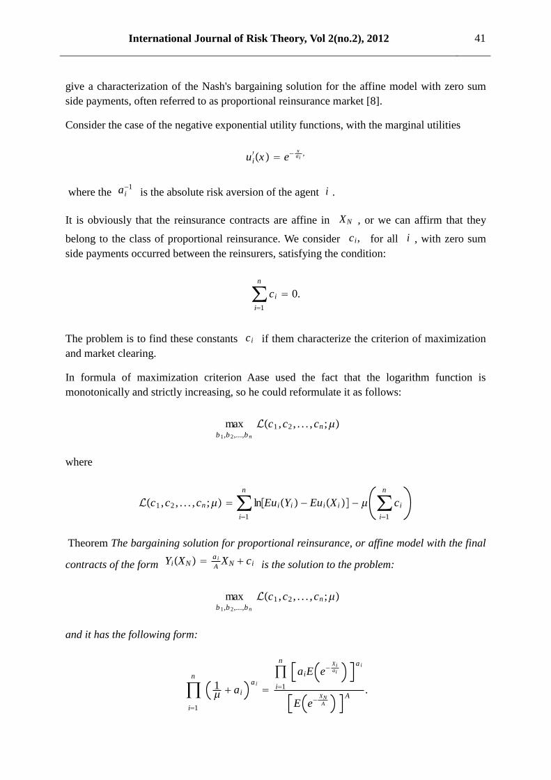
International Journal of Risk Theory, Vol 2(no.2), 2012 41
give a characterization of the Nash's bargaining solution for the affine model with zero sum
side payments, often referred to as proportional reinsurance market [8].
Consider the case of the negative exponential utility functions, with the marginal utilities
uix e
xai
,
where the ai1
is the absolute risk aversion of the agent i .
It is obviously that the reinsurance contracts are affine in XN , or we can affirm that they
belong to the class of proportional reinsurance. We consider ci, for all i , with zero sum
side payments occurred between the reinsurers, satisfying the condition:
i1
n
ci 0.
The problem is to find these constants c i if them characterize the criterion of maximization
and market clearing.
In formula of maximization criterion Aase used the fact that the logarithm function is
monotonically and strictly increasing, so he could reformulate it as follows:
b 1,b 2,...,b n
max Lc1 ,c2 , . . . ,cn ;
where
Lc1 ,c2 , . . . ,cn ; i1
n
lnEuiYi EuiX i i1
n
ci
Theorem The bargaining solution for proportional reinsurance, or affine model with the final
contracts of the form YiXN a i
AXN ci is the solution to the problem:
b 1,b 2,...,b n
max Lc1 ,c2 , . . . ,cn ;
and it has the following form:
i1
n
1 ai
a i
i1
n
aiE eXiai
a i
E eXNA
A.
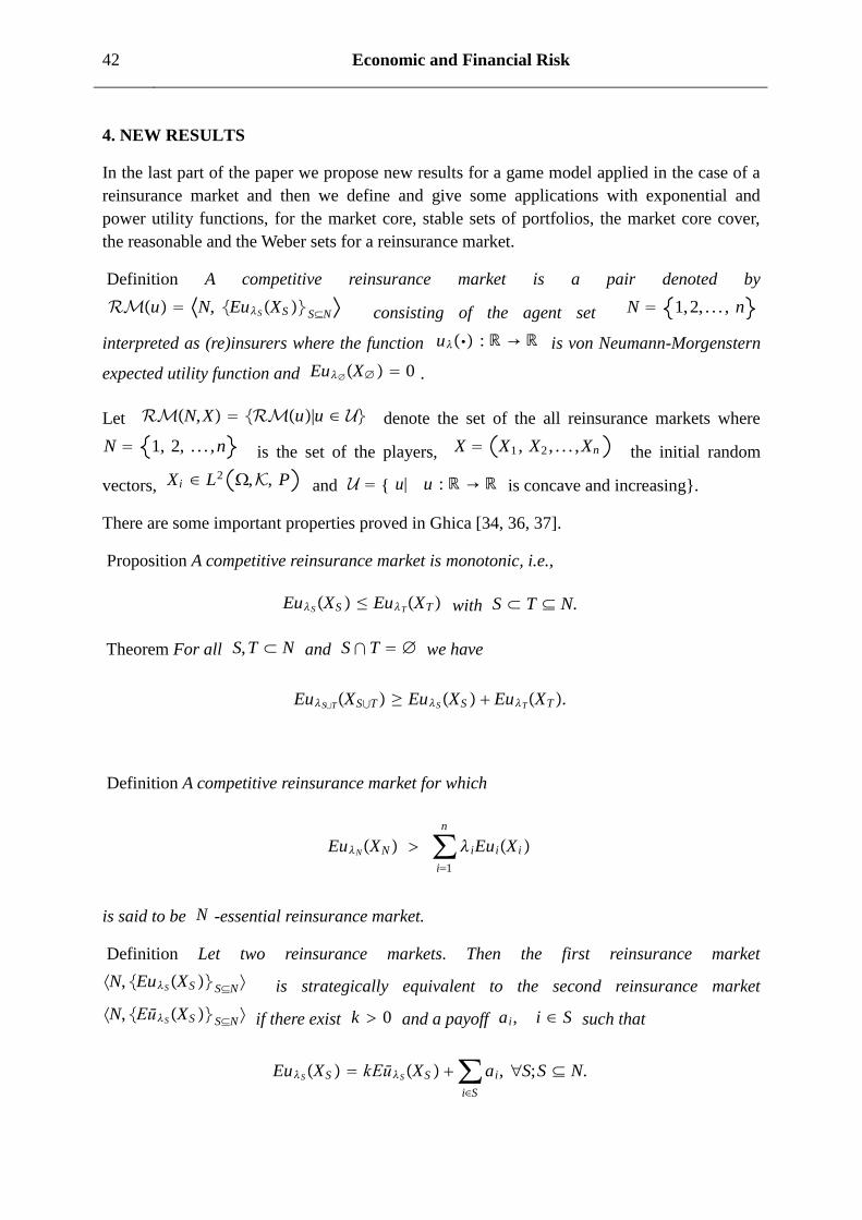
42 Economic and Financial Risk
4. NEW RESULTS
In the last part of the paper we propose new results for a game model applied in the case of a
reinsurance market and then we define and give some applications with exponential and
power utility functions, for the market core, stable sets of portfolios, the market core cover,
the reasonable and the Weber sets for a reinsurance market.
Definition A competitive reinsurance market is a pair denoted by
RMu N, EuSXS SN consisting of the agent set N 1,2, . . . , n
interpreted as (re)insurers where the function u : is von Neumann-Morgenstern
expected utility function and EuX 0 .
Let RMN,X RMu|u U denote the set of the all reinsurance markets where
N 1, 2, . . . ,n is the set of the players, X X1 , X2 , . . . ,Xn the initial random
vectors, Xi L2 ,K, P and U { u| u : is concave and increasing}.
There are some important properties proved in Ghica [34, 36, 37].
Proposition A competitive reinsurance market is monotonic, i.e.,
EuSXS EuTXT with S T N.
Theorem For all S,T N and S T we have
EuSTXST EuSXS EuTXT.
Definition A competitive reinsurance market for which
EuNXN i1
n
iEuiX i
is said to be N -essential reinsurance market.
Definition Let two reinsurance markets. Then the first reinsurance market
N,EuSXS SN is strategically equivalent to the second reinsurance market
N,EūSXS SN if there exist k 0 and a payoff a i, i S such that
EuSXS kEūSXS iS
ai, S;S N.
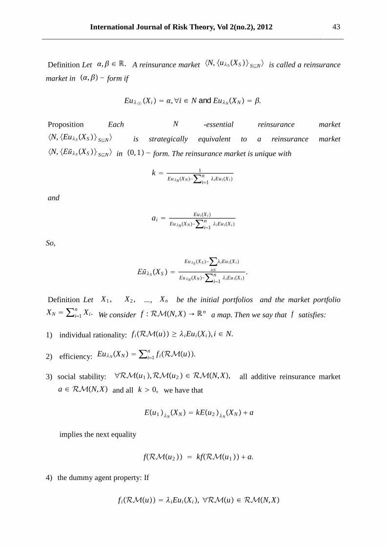
International Journal of Risk Theory, Vol 2(no.2), 2012 43
Definition Let , . A reinsurance market N,uSXS SN is called a reinsurance
market in , form if
EuiXi ,i N and EuNXN .
Proposition Each N -essential reinsurance market
N,EuSXS SN is strategically equivalent to a reinsurance market
N,EūSXS SN in 0,1 form. The reinsurance market is unique with
k 1
EuNXNi1
niEu iX i
and
ai
Eu iX i
EuNXNi1
niEu iX i
So,
EūSXS
EuSXS iS
iEu iX i
EuNXNi1
n iEu iX i
.
Definition Let X1 , X2 , ..., Xn be the initial portfolios and the market portfolio
XN i1
nXi. We consider f : RMN,X n
a map. Then we say that f satisfies:
1) individual rationality: f iRMu iEuiXi, i N.
2) efficiency: EuNXN i1
nf iRMu.
3) social stability: RMu1 ,RMu2 RMN,X, all additive reinsurance market
a RMN,X and all k 0, we have that
Eu1 NXN kEu2 N
XN a
implies the next equality
fRMu2 kfRMu1 a.
4) the dummy agent property: If
f iRMu iEuiXi, RMu RMN,X
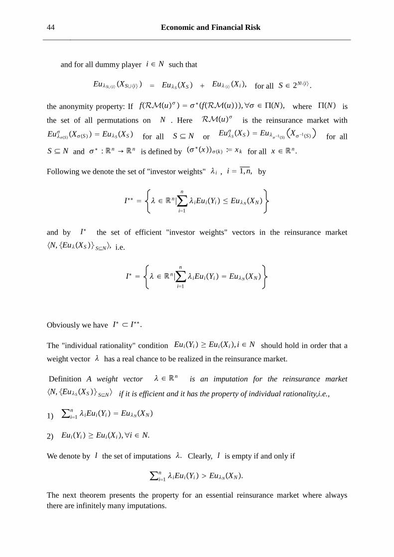
44 Economic and Financial Risk
and for all dummy player i N such that
EuSiXSi EuSXS EuiXi, for all S 2N\i.
the anonymity property: If fRMu fRMu, N, where N is
the set of all permutations on N . Here RMu is the reinsurance market with
EuS XS EuSXS for all S N or
EuS
XS Eu1S
X1S for all
S N and : n n is defined by xk : x k for all x n .
Following we denote the set of "investor weights" i , i 1,n, by
I n |i1
n
iEuiYi EuNXN
and by I the set of efficient "investor weights" vectors in the reinsurance market
N,EuXS SN, i.e.
I n |i1
n
iEuiYi EuNXN
Obviously we have I I.
The "individual rationality" condition EuiYi EuiXi, i N should hold in order that a
weight vector has a real chance to be realized in the reinsurance market.
Definition A weight vector n is an imputation for the reinsurance market
N,EuSXS SN if it is efficient and it has the property of individual rationality,i.e.,
1) i1
n iEuiYi EuNXN
2) EuiYi EuiXi,i N.
We denote by I the set of imputations . Clearly, I is empty if and only if
i1
n iEuiYi EuNXN.
The next theorem presents the property for an essential reinsurance market where always
there are infinitely many imputations.
International Journal of Risk Theory, Vol 2(no.2), 2012 45
Moreover, I is a simplex with extreme points the next vectors: f1 , f2 , . . . , fn for i N
where fi f1
i , f2i , . . . , fn
i defined by:
f ji
iEuiX i , if i j
EuNXN kNi
kEukXk , if i j
Theorem Let N,EuSXS SN be a reinsurance market . If the market
N, EuSXS SN is an essential market, then
1) I is an infinite set.
2) I is a convex hull of the points f1 , f2 , . . . , fn .
5. SOME GAME THEORY'S SETS STUDIED FOR A REINSURANCE MARKET
Because the set of imputations is too large for an essential reinsurance market, so, we need
some criteria to single out those imputations who have the chance to appear. So, we could
obtain some subsets of I as solution concepts. One of this solution concept is the core of a
reinsurance market.
Definition The market core denoted by MC of a reinsurance market
N, EuSXS SN is the set
MC I|iS
iEuiYi EuSXS ,S N
If MC then the elements of MC can easily be obtained because the core is defined
with the aid of a finite system of inequalities.
We introduce a set related on the market core namely: the market core cover. We can refer on
it like a "market core catcher" because it contains the market core as a subset.
We denote with M the upper allocation and with m the lower allocation who is important
for definition the new element. For each i N , the i -th coordinate Mi of the upper vector
M is the marginal contribution of the reinsurer i in the grand group of agents; it is also
called the utopia payoff for reinsurer i in the grand group of agents in the sense that if the
reinsurer i wants more then it is advantageous for the other agents in N to throw agent i
out.
46 Economic and Financial Risk
Definition Let N,EuSXS SN be a reinsurance market. For each i N and for each
S N with i S the marginal contribution of agent i to the coalition S is
MiS EuSXS EuS\iXS\i
Definition Let S N, i S. The remainder RS, i of reinsurer i in the group of agents
S is the amount which remains for reinsurer i if group of agents S forms and all other
agents in S obtain their utopia payoffs, i.e.,
RS, i : EuSXS jS\i
Mj
and for each i N, the i -th coordinate m i of the lower vector m is then defined by
m i :S; Si
max RS, i
Definition For a reinsurance market N, EuSXS SN the market core cover consists
of all weight vectors for which we have
MCC I| m i iEuiYi Mi, i N .
That MCC is a core catcher follows from the next theorem which presents that the lower
(upper) vector is a lower (upper) bound for the market core.
Theorem Let N,EuSXS SN be a reinsurance market and MC. Then
m i iEuiYi Mi, i N.
To describe a new kind of the set we will use the same notation: S i1, i2
, ...,is
where we have the set S i1 , i2 , ...,is and |S| s. In what it follows we present
another market core catcher: the reasonable set. This set was introduced in game theory by
Milnor in 1952.
Definition The reasonable set R of the reinsurance market denoted by
N,EuSXS SN is the set
R iN
R i
where, for i N, R i has the next form:
n | iEuiX i iEuiYi S; Si
max EuSXS EuS\iXS\i .
International Journal of Risk Theory, Vol 2(no.2), 2012 47
Remark Obviously MC MCC R.
The last market core catcher presented here correspond to the Weber set from game theory
[49].
Definition The Weber set W of the reinsurance market denoted by
N,EuSXS SN is the convex hull of the n! marginal vectors m , corresponding to
the n! permutations N :
m1
Z1Z1X1
sup 1Eu1Z1
m2
Z1,Z2Z1Z2X1X2
sup Eu1,2Z1,2
Z1
Z1X1
sup 1Eu1 Z1
. . . . . . . . . . . . . . . . . . . . . . . . . . . . . . .
mk
Z1,..,ZkZ1...ZkX1...Xk
sup Eu1,...,kZ1,...,k
Z1,..,Zk1
Z1...Zk1X1...Xk1
sup Eu1,...,k1Z1,...,k1
for each k N.
The payoff vector m can be created as follows. Let the agents enter in a room one by one in
the order: 1, . . . ,n and give each agent the marginal contribution which he creates by
entering.
We propose in the following a result who is necessary for proving the next theorem.
Proposition The set MC is a convex set.
The Weber set is a market core catcher as shown in the next theorem. We will prove that
MC W.
Theorem Let N,EuSXS SN be the reinsurance market. Then MC W.
48 Economic and Financial Risk
6. SOME APPLICATIONS. THE EXPONENTIAL UTILITY FUNCTION
In general the core will be characterized by the Pareto optimal allocations according to
investor weights i in some region restricted by inequalities given in the following
theorems.
The initial portfolios are denoted by X1 ,X2 , . . ,Xn , the " market portfolio" is XN i1
nXi
and the reinsurers have the exponential utility functions given by: uix 1 aie x
ai ,
x , i N.
From Aase The Pareto optimal allocations who result from coalition are [2, 3]:
YiXN a i
AXN biN, where biN ai lni ai
K
A, A
i1
nai and
K i1
nai lni
and for any subset S N the formulas from above becomes:
YiXS a i
ASXS biS,
Where
biS ai lni aiKS
AS, AS iS
ai , KS iSai lni, XS iS
Xi
The values i appear as "investor weights" are arbitrary positive constants and we want to
find the constraints for the values sets of these constants, or equivalently, to deceive
constraints on the zero-sum side payments b i.
We use for these requirements the expected utility of the representative agents for any
S N :
EuSXS E
iS
i ASeKSXS
AS
We can see that the market core is characterized by the Pareto optimal allocations
corresponding to investor weights i in some region restricted by inequalities of the above
kind, in general a polyhedron from intn .
Theorem The Pareto optimal allocations who correspond to the market core cover are given
by weights i, i N , the solutions of the system of next inequalities:
i i i, i N,
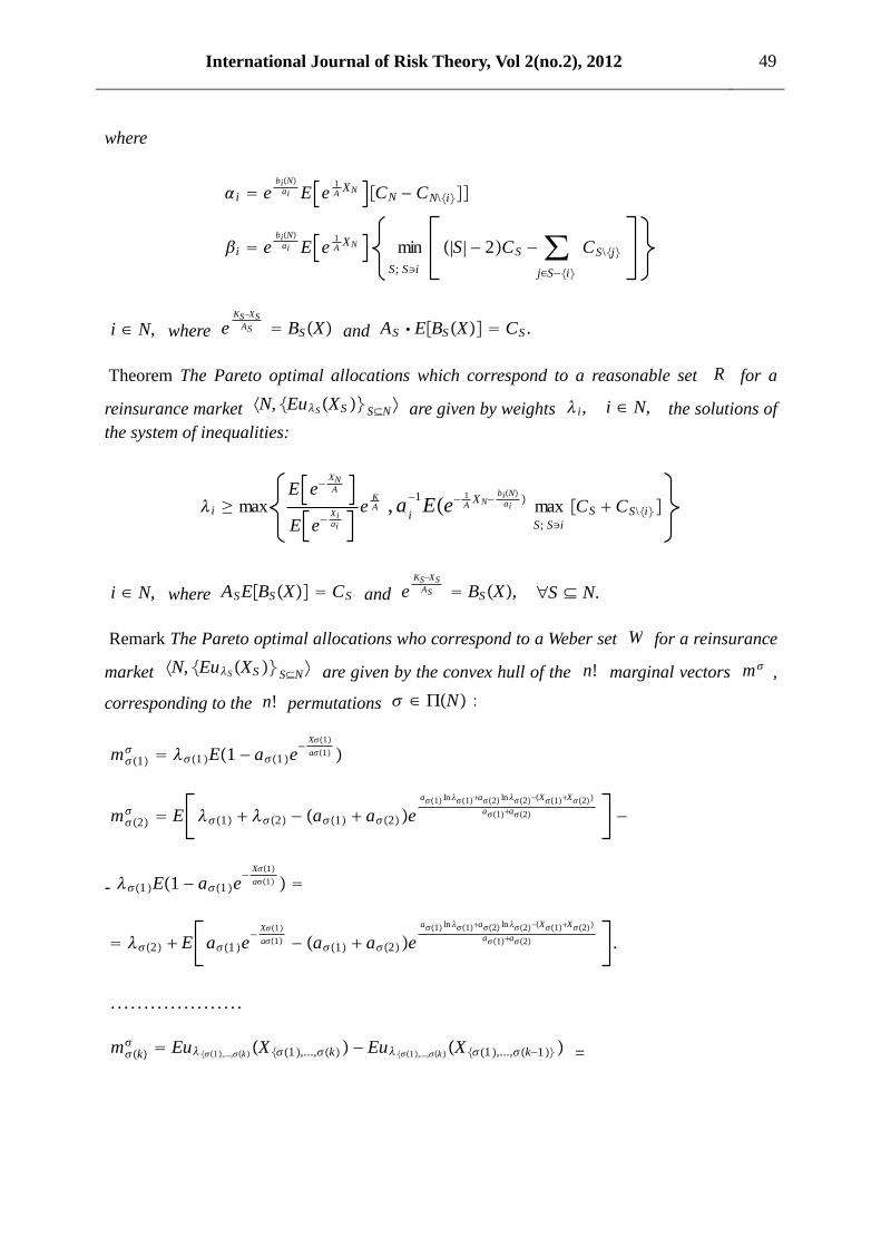
International Journal of Risk Theory, Vol 2(no.2), 2012 49
where
i ebiN
ai E e1A
XN CN CN\i
i ebiN
ai E e1A
XN
S; Si
min |S| 2CS jSi
CS\j
i N, where eKSXS
AS BSX and AS EBSX CS .
Theorem The Pareto optimal allocations which correspond to a reasonable set R for a
reinsurance market N,EuSXS SN are given by weights i, i N, the solutions of
the system of inequalities:
i maxE e
XNA
E eXiai
eKA , a
i
1Ee
1A
XNbiN
ai
S; Si
max CS CS\i
i N, where ASEBSX CS and eKSXS
AS BSX, S N.
Remark The Pareto optimal allocations who correspond to a Weber set W for a reinsurance
market N,EuSXS SN are given by the convex hull of the n! marginal vectors m ,
corresponding to the n! permutations N :
m1 1E1 a1e
X1
a1
m2
E 1 2 a1 a2ea1 ln1a2 ln2X1X2
a1a2
- 1E1 a1e X1
a1
2 E a1e
X1
a1 a1 a2ea1 ln1a2 ln2X1X2
a1a2 .
. . . . . . . . . . . . . . . . . . . .
mk Eu1,...,kX1,...,k Eu1,...,kX1,...,k1 =
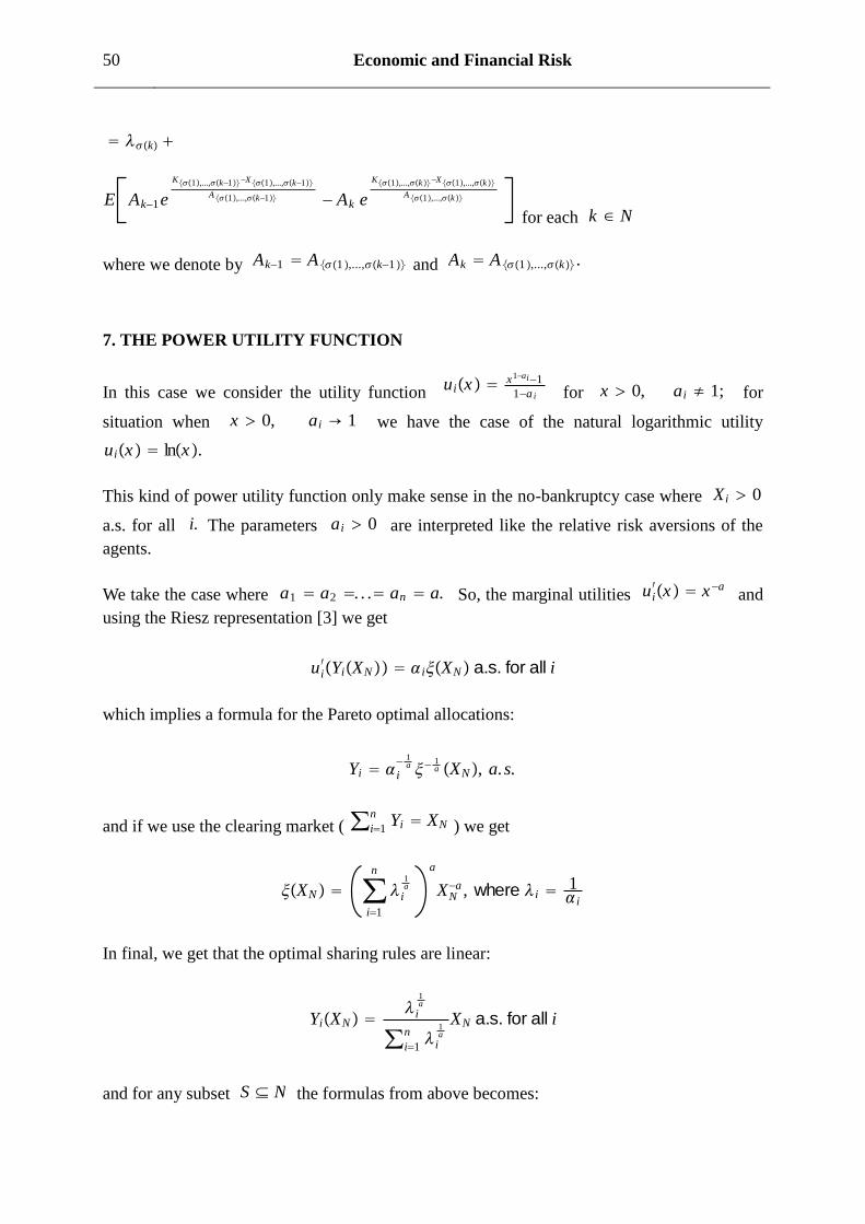
50 Economic and Financial Risk
k
E Ak1e
K1,...,k1X1,...,k1A1,...,k1 Ak e
K1,...,kX1,...,kA1,...,k
for each k N
where we denote by Ak1 A1,...,k1 and Ak A1,...,k.
7. THE POWER UTILITY FUNCTION
In this case we consider the utility function uix x1ai1
1a i for x 0, ai 1; for
situation when x 0, ai 1 we have the case of the natural logarithmic utility
uix lnx.
This kind of power utility function only make sense in the no-bankruptcy case where Xi 0
a.s. for all i. The parameters ai 0 are interpreted like the relative risk aversions of the
agents.
We take the case where a1 a2 . . . an a. So, the marginal utilities uix xa
and
using the Riesz representation [3] we get
uiYiXN iXN a.s. for all i
which implies a formula for the Pareto optimal allocations:
Yi i
1a
1a XN, a.s.
and if we use the clearing market ( i1
nYi XN ) we get
XN i1
n
i
1a
a
XNa , where i 1
i
In final, we get that the optimal sharing rules are linear:
YiXN i
1a
i1
n i
1a
XN a.s. for all i
and for any subset S N the formulas from above becomes:
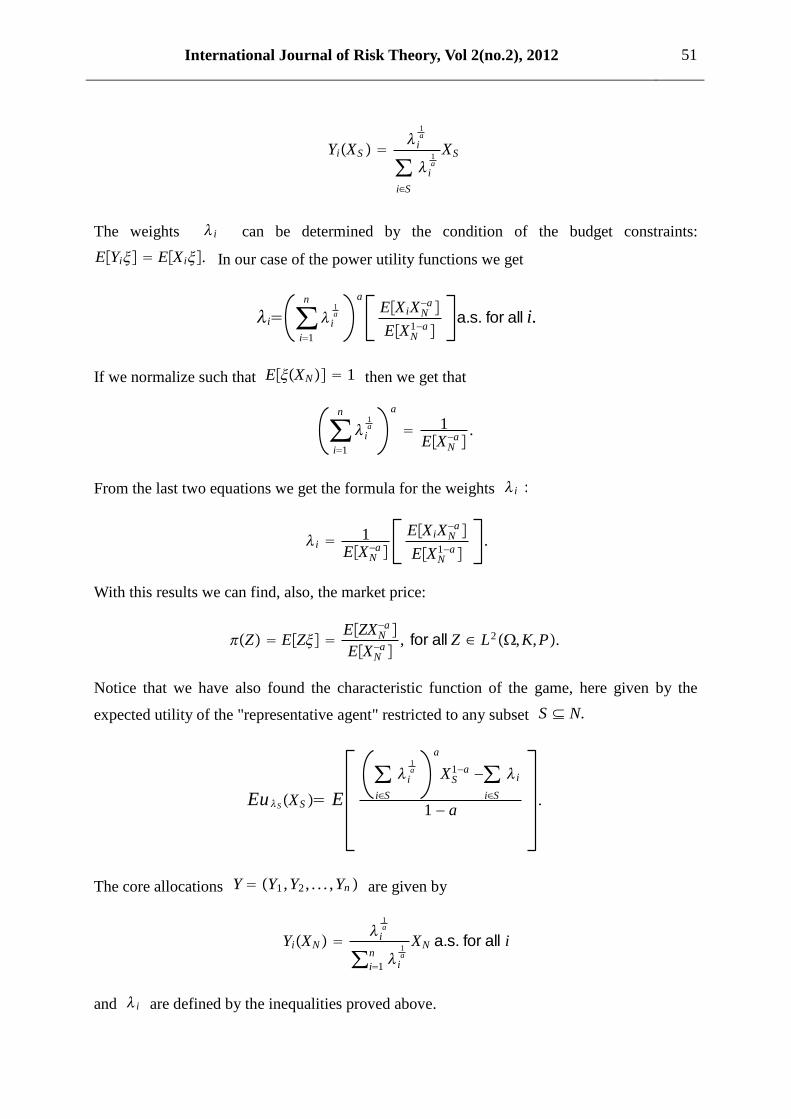
International Journal of Risk Theory, Vol 2(no.2), 2012 51
YiXS i
1a
iS
i
1a
XS
The weights i can be determined by the condition of the budget constraints:
EYi EXi. In our case of the power utility functions we get
i i1
n
i
1a
a
EX iXNa
EXN1a
a.s. for all i.
If we normalize such that EXN 1 then we get that
i1
n
i
1a
a
1EXN
a .
From the last two equations we get the formula for the weights i :
i 1EXN
a EX iXN
a
EXN1a
.
With this results we can find, also, the market price:
Z EZ EZXN
a EXN
a , for all Z L2,K,P.
Notice that we have also found the characteristic function of the game, here given by the
expected utility of the "representative agent" restricted to any subset S N.
EuSXS E iS
i
1a
a
XS1a
iS
i
1 a.
The core allocations Y Y1 ,Y2 , . . . ,Yn are given by
YiXN i
1a
i1
n i
1a
XN a.s. for all i
and i are defined by the inequalities proved above.

52 Economic and Financial Risk
Theorem The Pareto optimal allocations which correspond to the market core cover are
given by weights i i N, the solutions of the system of next inequalities:
i 1
E XN1a
S; Si
max 2 |S|a,SEXS1a
jSi
a,S\jE XS\j1a
i E XN
1a
E XNa a,N\iE XN\i
1a
E XN1a
where
iS
i
1a
a
a,S ,S N.
Theorem The Pareto optimal allocations who correspond to a reasonable set R for a
reinsurance market N,EuSXS SN are given by weights i i N, the solutions of
the system of inequalities:
i maxR1X,R2X
with
R1,iX EXN
1a
EX i1a
EXNa and
R2,iX S; Si
max a,SEXS1a a,S\iE XS\i
1a
a
EXN1a EXN a
.
Remark The Pareto optimal allocations who correspond to a Weber set W for a reinsurance
market N,EuSXS SN are given by the convex hull of the n! marginal vectors m ,
corresponding to the n! permutations N :
m1
1
1aEX1
1a 1
m2
E 1 2 a1 a2ea1 ln1a2 ln2X1X2
a1a2
- 1E1 a1e X1
a1
2
1a 1
1aE 1
1/a 21/a a
X1 X21a 1X1
1a
International Journal of Risk Theory, Vol 2(no.2), 2012 53
. . . . . . . . . . . . . . . . . . . .
mk EuX1,...,k EuX1,...,k1 =
kE
a, 1,..kX1...Xk
1aa, 1,..k1
X1...Xk1 1a
1a
for each k N,
where
a,1,..k i1,..k
i
1a
a
.
8. CONCLUSIONS
An important part of the actuarial mathematics is constituted by elements of mathematical
stochastic, in particular theories like: probability theory, statistical theory or risk theory. In
many cases the conditions and the assumptions for the assessment of risk sharing or
equilibrium market are by far less favorable. As we presented in this paper, few authors
showed that original objectives of game theory was to analyze markets in many particular
forms, situations when the assumptions behind the neoclassical competitive equilibrium
appears unreasonable.
Despite of the fact that the most researches in life insurance mathematics are sustained by the
theory of risk there are difficulties to put in the practice the results like competitive
equilibrium, Pareto optimality, representative agent pricing and its implications for insurance
premiums. We presented in this paper an alternative model based on game theoretic approach
and we have tried to show that game theory can be applied to a number of problems in
insurance, problems with unsatisfactory results in other theories who belong to general
economic theory or to a stochastic theory.
REFERENCES
[1] Aase, K.K. Premium in a Dynamic Model of a Reinsurance Market, Scand. Actuarial
Journal, 1993a.
[2] Aase, K.K. Equilibrium in a Reinsurance Syndicate; Existance, Uniqueness and
Characterization, ASTIN Bulletin 22,2, 1993b, 185-211.
[3] Aase, K.K. Perspectives of Risk Sharing, Scand. Actuarial Journal 2, 2002, 73-128.
[4] Aase, K.K. Optimal Risk Sharing, In J. L. Teugels& B. Sundt (Eds.) Encyclopedia of
actuarial science vol 3, 2004a, 1212-1215, Chichester, UK: Wiley.
[5] Aase, K.K. A Pricing Model for Quantity Contracts, The Journal of Risk and Insurance,
54 Economic and Financial Risk
vol 71, 4, 2004b, 617- 642.
[6] Aase, K.K. Equilibrium in Marine Mutual Insurance Markets with Convex Operating
Costs, The Journal of Risk and Insurance, vol 74, 1, 2007, 239-268.
[7] Aase, K.K. Existance and Uniqueness of Equilibrium in a Reinsurance Syndicate,
Norvegian School of Economics and Business Administration, Department of Finance and
Management Science, 2008.
[8] Aase, K.K. The Nash Solutions Bargaining Solution vs. Equillibrium in a Reinsurance
Syndicate, Scand. Actuarial Journal 3, 2009, 219-238.
[9] Araujo, A and Monteiro, P.K. Equillibrium Without Uniform Conditions J. Econ. Theory,
48, 1989, 416-427.
[10] Arrow, K.J. The Role of Securities in the Optimal Allocation of Risk-Bearing,
Econometrie, as translated and reprinted in 1964, Review of Economic, studies, 31, 1953, 6-
91.
[11] Arrow, K.J. The Theory of Risk-Bearing: Small and Great Risks, Journal of Risk and
Uncertainty 12, 1996, 103-111.
[12] Arrow, K.J. and Debreu, G. Existance of an Equillibrium for a Competitive Economy,
Econometrica, 22, 1954, 265-290.
[13] Aumann, R. J. and Mascheler, M. The Bargaining Set for Cooperative Games, Annals of
Mathematical Studies 52, 1964, 443-476.
[14] Aumann, R. J. Disadvantageous Monopolies, J. of Economic Theory, 6, 1973, 1-11.
[15] Baton, B. and Lemaire, J. The Core of a Reinsurance Market, ASTIN Bulletin 12,1,
1981a, 57-71.
[16] Baton, B. and Lemaire, J. The Bargaining Set of a Reinsurance Market, ASTIN Bulletin
12, 2, 1981b, 101-114.
[17] Borch, K. The Safety Loading of Reinsurance Premiums, Skadinavisk Aktuarietidskrift,
1960a, 163-184.
[18] Borch, K. Reciprocal Reinsurance Treaties Seen as a Two-person Cooperative Game,
Skadinavisk Aktuarietidskrift 43, 1960b, 29-58.
[19] Borch, K. Reciprocal Reinsurance Treaties, ASTIN Bulletin, 1, 1960c, 170-191.
[20] Borch, K. The utility concept applied to the theory of insurance, ASTIN Bulletin, 1,
1961, 245-255.
[21] Borch, K. Application of Game Theory to Some Problems in Automobile Insurance,
ASTIN Bulletin 2, 1962, 208-221.
International Journal of Risk Theory, Vol 2(no.2), 2012 55
[22] Borch, K. Recent Developments in Economic Theory and Their Aplication to Insurance,
ASTIN Bulletin 2, 1963, 322-341.
[23] Borch, K. The Theory of Risk Journal of the Royal Statistical Society, Series B 29, 1967,
432-453.
[24] Borch, K. A Note on Uncertainty and Indifference Curves, Rev. Econ. Stud., 1969, 1-4.
[25] Borch, K. The Mathematical Theory of Insurance , D. C. Heath: Lexington, MA, 1974.
[26] Bühlmann, H. Mathematical Methods in Risk Theory, Springer -Verlag, New York, 1970.
[27] Buhlmann, H. and Jewell, W.S. Ooptimal Risk Exchanges, ASTIN Bulletin, 10, 1979,
243-262.
[28] Davis, M. and Mascheler, M. The Kernel of the Cooperative Games Naval Research
Logistics Quarterly 12, 1965, 223-259.
[29] Debreu, G. Une Economie de l'Incertain, Miméo Électricité de France, 1953.
[30] Debreu, G. and Scarf H. A Limit Theorem on the Core of an Economy, International
Economic Review 4, 1963, 235-246.
[31] Du Mouchel, W. The Pareto-Optimality of an n-Company Reinsurance Treaty,
Skandinavisk Aktuarietidskrift 51, 1968, 165-170.
[32] Garven, J.R. and Lamm-Tennant, J. The Demand for Reinsurance: Theory and Empirical
Tests , Insurance and Risk Management, 71(2), 2003, 217-237.
[33] Gerber, H. An Introduction to Mathematical Risk Theory, Huebner Foundation
Monograph, Wharten School, University of Pennsylvania, 1979.
[34] Ghica, M. The Core of a Reinsurance Market, Mathematical Reports 10(60), 2, 2008,
155-164.
[35] Ghica, M. Portfolio optimization. A Game Approach in a Reinsurance Market, Ed
Universitătii Bucuresti, 2011.
[36] Ghica, M. A Game Theoretic Model for a Reinsurance Market. Some Theoretical results,
Mathematical Reports, 2013a, submitted.
[37] Ghica, M. Market cores and stable sets for a reinsurance market, Proceedings of the
Romanian Academy, 2013b, submitted.
[38] Kihlstrom, R. and Pauly, M. The Role of Insurance in the Allocation of Risk, American
Economic Review, 61, 1971, 371-379.
[39] Kihlstrom, R. and Roth, A.E. Risk Aversion and the Negotation of Insurance Contracts,
Journal of Risk and Insurance, 49, 1982, 372-387.
56 Economic and Financial Risk
[40] Lemaire, J. Echange de Risques entre Assureurs et Theorie des Jeux, ASTIN Bulletin, 9,
1977, 155-180.
[41] Lemaire, J. A non-Simmetrical Value for Games without Transferable Utilities.
Application to Reinsurance, ASTIN Bulletin, 10, 1979, 195-214.
[42] Lemaire, J. Cooperative Game Theory and its insurance Applications, ASTIN Bulletin,
21, 1990a, 17-40.
[43] Lemaire, J. Borch's theorem, In Louberge, H. (ed) Risk, Information and insurance.
Essays in the Memory of Karl h. Borch. Kluwer Academic Publisher, Boston, London, 1990b,
15-37.
[44] Lucas W. Game Theory and its Applications Proceedings of Symposia in Applied Maths
24, American Math. Soc.: Providence, 1981.
[45] Maschler, M. The Bargaining Set, Kernel and Nucleolus, in R. J. Aumann and S. Hart
(eds.), Handbook of Game Theory, Vol I (Amsterdam: Elsevier), 1992, 591-665.
[46] Owen, G. Game Theory Academic Press: Orlando, FL, 1982.
[47] von Neumann, J. and Morgenstern, O. Theory of Games and Economic Behaviour,
Princeton University Press, 1944.
[48] Schmeidler, D. The Nucleolus of a Characterstic Function Game SIAM Journal of
Applied Maths, 1969, 1163-1170.
[49] Weber, R. Probabilistic Values for Games, in: Roth, A.E. (Ed.), The Shapley Value:
Essays in Honour of Lloyd S. Shapley, Cambridge University Press, 1988, 101-119.
International Journal of Risk Theory, Vol 2(no.2), 2012 57
BLACK-SCHOLES MODEL AND GARCH PROCESSES
WITH RISK MANAGEMENT
Muhammad Sheraz1
1 Doctoral School of Mathematics, Faculty of Mathematics
and Computer Science, University of Bucharest, Romania
ABSTRACT
The Black-Scholes option pricing model is a mathematical description of financial market and derivative
investment instrument. In BS-model volatility is a constant function where trading option is indeed, risky due to
random component such as volatility. Bs-model can be used to derive the hedging strategies. The concept of non
constant volatility has been introduced in GARCH processes. Time varying volatility is a natural extension of the
diffusion models widely applied in the asset pricing literature (Hull-White). Jump processes are characterized by
discontinuous development of the analyzed random variable. In this paper a BS-model with jump has been
considered to calculate the Greeks of the model and to prove that model’s call option is a monotonous function in
volatility. Finally the concepts of locally risk natural value relationship (LRNVR) and GARCH option pricing are
discussed.
KEYWORDS
Option Pricing, Black-Scholes model, Jump diffusion process, LRNVR, GARCH Processes.
1. INTRODUCTION
Equally spaced increments are stationary in Brownian motion that is it can be assumed that
they are independently and identically distributed, but the most of the empirical studies shows
that this is generally not true. The introduction of stochastic volatility in stock prices, refine
the pricing of derivative instruments. In 1973 Black and Scholes introduced that, the option is
implicitly priced if the stock is traded [1]. The Black-Scholes option pricing model is a
mathematical description of financial market and derivative investment instrument. The model
has some contradictory assumptions, for example the model assumes that volatility of the
asset remain constant while empirical studies shows that generally this is not the case and
constant volatility model is not adequate for the log returns. These pricing errors resulting
from unrealistic assumption of the model have serious consequences for measuring the risk of
portfolios [9]. Risk measurement is becoming more and more important in the financial risk
management of banks and other institutions involved in financial markets. The need to
quantify risk typically arises when a financial institution has to determine the amount of
capital to hold as a protection against unexpected losses. In fact, risk measurement is
concerned with all types of risks encountered in finance. Market risk, the best-known type of
risk, is the risk of change in the value of a financial position.
Trading options is particularly risky due to the possibly high random component. An option
pricing formula was derived for the more general case when the underlying stock exchanges
are generated by a mixture of both continuous and jump process [10]. Advanced strategies to
58 Economic and Financial Risk
reduce and manage this risk can be derived from the Black–Scholes formula. An expensive
hedging strategy, i.e. a strategy to decrease the risk associated with the sale of a call, is the so
called stop–loss strategy: The bank selling the option takes an uncovered position as long as
the stock price is below the exercise price, < , and sets up a covered position as soon as
the call is in–the–money, > . The shares to be delivered in case of options exercise are
bought as soon as the stock trades above the exercise price , and are sold as soon as
falls below the exercise price . Since all stocks are sold and bought at after time 0 and at
maturity T either the stock position is zero, ( < ), or the stocks are sold at to the option
holder, ( > , this strategy bears no costs. In order to apply the concept of risk neutral
valuation (see Cox and Ross (1976)) the probability measure has to be transformed such that
the price process under this new measure is a martingale. In incomplete markets, however, a
multitude of such transformations exist, Harrison and Kreps (1979). In contrast to complete
markets the trader cannot build up a self–financing portfolio reproducing the options payoff at
maturity when the market is incomplete. Therefore hedging is no longer risk free, and option
prices depend on risk preferences.
The notion of non constant volatility has been introduced by GARCH processes [3]. The study
of stock price models under GARCH volatility is a new horizon in derivative investment
instruments. Duan (1995) was the first to provide a solid theoretical foundation for GARCH
option pricing [5]. Duan generalize the concept of risk neutral valuation and introduced the
notion of Locally Risk Neutral Valuation Relationship (LRNVR), which provides a solid
economic argument to choose a particular equivalent martingale measure under the GARCH
model with conditionally Normal innovations. Duan model contain the Black-Scholes model
as a special case of homoskedasticity and it has been proved that the discounted price
processes for underlying asset is a martingale measure under . In Duan GARCH option
pricing model, the conditional variance process of the underlying asset under the risk
neutralized pricing probability specified by LRNVR is a nonlinear asymmetric GARCH
model.
In this article section 2 is consisting of a general frame work for the famous Black-Scholes
option pricing model. In section 3 using more general case of BS-formula with jump, the
Greeks for the model have been obtained and it is also shown that model’s call option is
monotonous function in volatility. In section 4 the notion of locally risk natural value
relationship (LRNVR) and GARCH model for option pricing has been studied. Finally section
5 is consisting of conclusions.
2. PRICING EUROPEAN OPTIONS
In finance, a derivative is a financial instrument whose value depends on other underlying
variables and such variables can be price of other financial instruments (underlying asset) like
interest rates, volatilities and indices. A European option is a derivative which at some
terminal time has a value given by some known functions of the asset prices at time .
A European call option is a contract that gives it holder the right, but not the obligation to buy
International Journal of Risk Theory, Vol 2(no.2), 2012 59
one unit of an underlying asset for a predetermined strike price on the maturity date . If
is a price of underlying asset at maturity then value of this contract at maturity will be
or
Here in the first case the holder will exercise the option and make a portfolio by
buying the stock for and selling it immediately at market price , while in the second case
the option is not exercised.
Similarly a European put option is a contract that gives its holder the right to sell a unit of
asset for strike price at then payoff is
or
At time this contract has a value known as the derivative price. Black and Scholes used
the model for Stock prices
Let be the risk free interest rate. The probability measure is called an equivalent
martingale measure to probability measure and we can write
According to fundamental theorem of asset pricing an arbitrage free price of an option at
time is
And
For a European call option as described the Black-Scholes Partial Differential Equation is
solved with final condition . Let us denote the pricing of
European calls at time for an observed risky asset price some mathematical
calculations yields the closed form solution of Black-Scholes PDE.
in equation we obtain the explicit solution of European call option
(2.1)
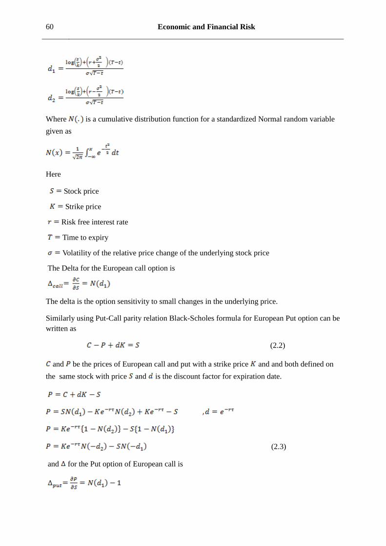
60 Economic and Financial Risk
Where is a cumulative distribution function for a standardized Normal random variable
given as
Here
Stock price
Strike price
Risk free interest rate
Time to expiry
Volatility of the relative price change of the underlying stock price
The Delta for the European call option is
The delta is the option sensitivity to small changes in the underlying price.
Similarly using Put-Call parity relation Black-Scholes formula for European Put option can be
written as
(2.2)
and be the prices of European call and put with a strike price and and both defined on
the same stock with price and is the discount factor for expiration date.
(2.3)
and for the Put option of European call is
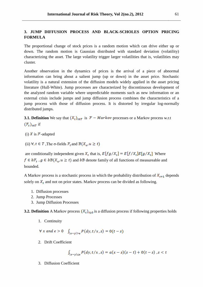
International Journal of Risk Theory, Vol 2(no.2), 2012 61
3. JUMP DIFFUSION PROCESS AND BLACK-SCHOLES OPTION PRICING
FORMULA
The proportional change of stock prices is a random motion which can drive either up or
down. The random motion is Gaussian distributed with standard deviation (volatility)
characterizing the asset. The large volatility trigger larger volatilities that is, volatilities may
cluster.
Another observation in the dynamics of prices is the arrival of a piece of abnormal
information can bring about a salient jump (up or down) in the asset price. Stochastic
volatility is a natural extension of the diffusion models widely applied in the asset pricing
literature (Hull-White). Jump processes are characterized by discontinuous development of
the analyzed random variable where unpredictable moments such as new information or an
external crisis include jumps and jump diffusion process combines the characteristics of a
jump process with those of diffusion process. It is distorted by irregular log-normally
distributed jumps.
3.1. Definition We say that is processes or a Markov process w.r.t
if
(i) is -adapted
(ii) ,The σ-fields and
are conditionally independent given that is, Where
and denote family of all functions of measureable and
bounded.
A Markov process is a stochastic process in which the probability distribution of depends
solely on and not on prior states. Markov process can be divided as following.
1. Diffusion processes
2. Jump Processes
3. Jump Diffusion Processes
3.2. Definition A Markov process is a diffusion process if following properties holds
1. Continuity
2. Drift Coefficient
3. Diffusion Coefficient
62 Economic and Financial Risk
Stochastic volatility models let volatility follow a diffusion process and the occasional
discontinuous jumps add more mass to the tails and help to match excess kurtosis in the
empirical distribution of stock returns. We suppose that jump is a Poisson random variable.
3.3. Definition A c dl g process is a Poisson process with parameter if
a. take values in and is a L vy process
b. , The increment has Poisson distribution of parameter
i.e
If is a Poisson distribution then
In addition is a L vy if it is c dl g with stationary independent increments
and for any
Further more if is a continuous real process with then following are
equivalent
(i) is Brownian motion
(ii) is L vy process
We have considered jump is Poisson random variable so we consider in time interval the
probability distribution for the number of jumps is and let is a jump indicator
function as
We say if a jump occurs then stock variable changes by amount
(3.1)
Here is another random variable and we say value of
i.e value of drops to zero and
International Journal of Risk Theory, Vol 2(no.2), 2012 63
otherwise
So change in value of a function and expected change in from
jump events at time is
Assuming that jump risk is not symmetric in order to use continuous modeling because
introduction of jump may eliminate continuous time modeling. Using Ito lemma for jump
diffusion processes, we can write
(3.2)
Here we can see that any stochastic process can be represented as combination of diffusion
and Poisson processes.
Rewriting equation (3.2) using above results
(3.3)
We know that we have set change in stock variable by occurrence of jump as and let
.
Where the expected gain or loss is conditional on jump so we obtain probability of jump
multiplied by returns given the jump is or so we can write
(3.4)
where is the total rate of return on stock. Rewriting equation (3.2)
(3.5)
Here can be symmetric jump risk is not continuously hedged, mixing options and stocks
to eliminate risk . Using It lemma again for jump diffusion
(3.6)
64 Economic and Financial Risk
The portfolio is consist of shares and written call with
(3.7)
Here
If
From (3.7) we get
( (3.8)
Equation (3.8) is similar as Black-Scholes PDE just replacing by .
Equation (2.1) of section 2 can be written as
(3.9)
( (3.10)
Equation (3.3) is similar with Black-Scholes Partial Differential Equation just replacing by
Following the equation (3.10) Black-Scholes Call Option can be written as
(3.11)
Theorem.3.1 The Greeks of BS-call option with jump corresponding to the equation (3.11)
are given by:
i. Delta=
International Journal of Risk Theory, Vol 2(no.2), 2012 65
ii. Gamma=
iii. Theta=
iv. Rho=
v. Vega=
Proof.
i.
where =
and ,
ii. =
iii.
=
where
iv.
v.
=
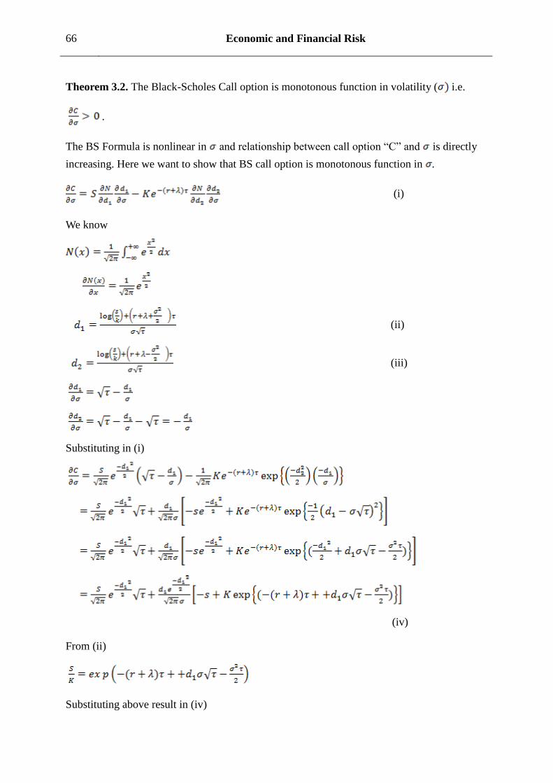
66 Economic and Financial Risk
Theorem 3.2. The Black-Scholes Call option is monotonous function in volatility ( i.e.
.
The BS Formula is nonlinear in and relationship between call option ―C‖ and is directly
increasing. Here we want to show that BS call option is monotonous function in .
(i)
We know
(ii)
(iii)
Substituting in (i)
(iv)
From (ii)
Substituting above result in (iv)
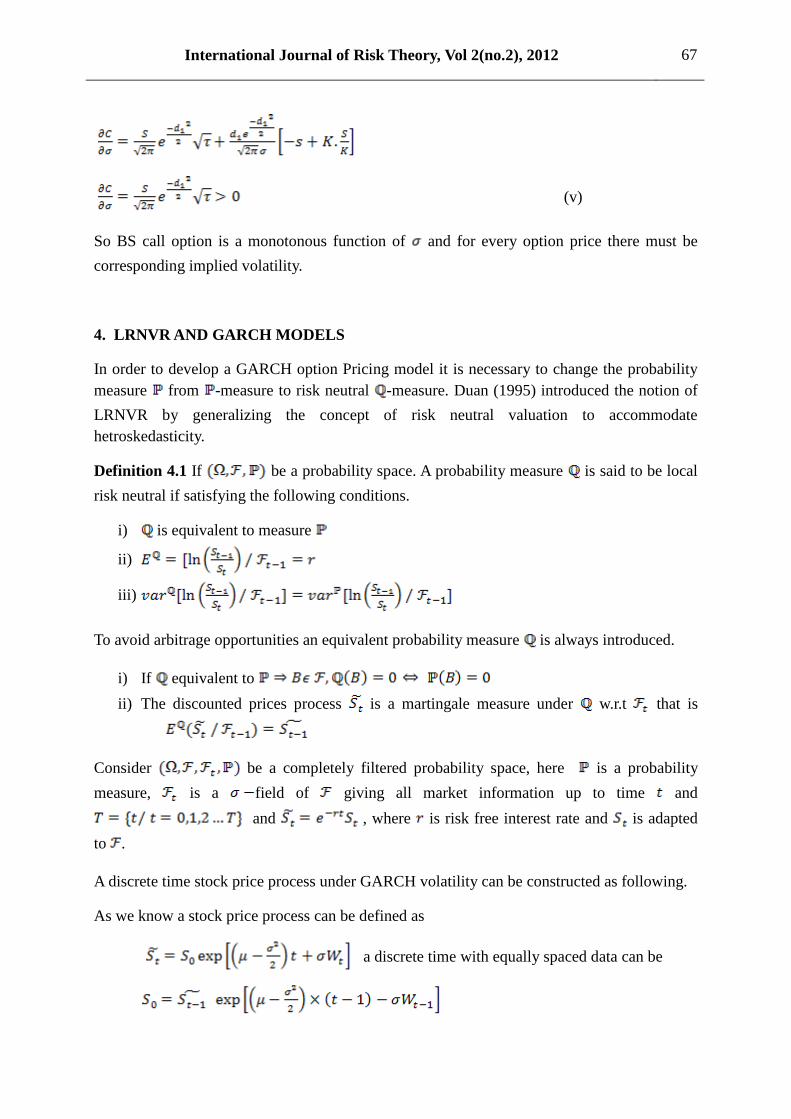
International Journal of Risk Theory, Vol 2(no.2), 2012 67
(v)
So BS call option is a monotonous function of and for every option price there must be
corresponding implied volatility.
4. LRNVR AND GARCH MODELS
In order to develop a GARCH option Pricing model it is necessary to change the probability
measure from -measure to risk neutral -measure. Duan (1995) introduced the notion of
LRNVR by generalizing the concept of risk neutral valuation to accommodate
hetroskedasticity.
Definition 4.1 If be a probability space. A probability measure is said to be local
risk neutral if satisfying the following conditions.
i) is equivalent to measure
ii)
iii)
To avoid arbitrage opportunities an equivalent probability measure is always introduced.
i) If equivalent to
ii) The discounted prices process is a martingale measure under w.r.t that is
Consider be a completely filtered probability space, here is a probability
measure, is a field of giving all market information up to time and
and , where is risk free interest rate and is adapted
to .
A discrete time stock price process under GARCH volatility can be constructed as following.
As we know a stock price process can be defined as
a discrete time with equally spaced data can be
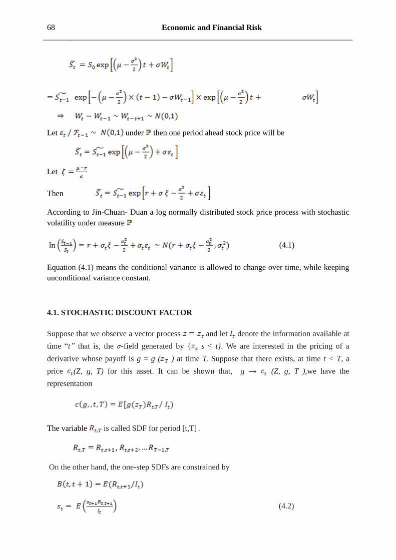
68 Economic and Financial Risk
Let under then one period ahead stock price will be
Let
Then
According to Jin-Chuan- Duan a log normally distributed stock price process with stochastic
volatility under measure
(4.1)
Equation (4.1) means the conditional variance is allowed to change over time, while keeping
unconditional variance constant.
4.1. STOCHASTIC DISCOUNT FACTOR
Suppose that we observe a vector process and let denote the information available at
time ―t” that is, the σ-field generated by { s ≤ t}. We are interested in the pricing of a
derivative whose payoff is g = g ( ) at time T. Suppose that there exists, at time t < T, a
price (Z, g, T) for this asset. It can be shown that, g → (Z, g, T ),we have the
representation
The variable is called SDF for period [t,T] .
,
On the other hand, the one-step SDFs are constrained by
(4.2)
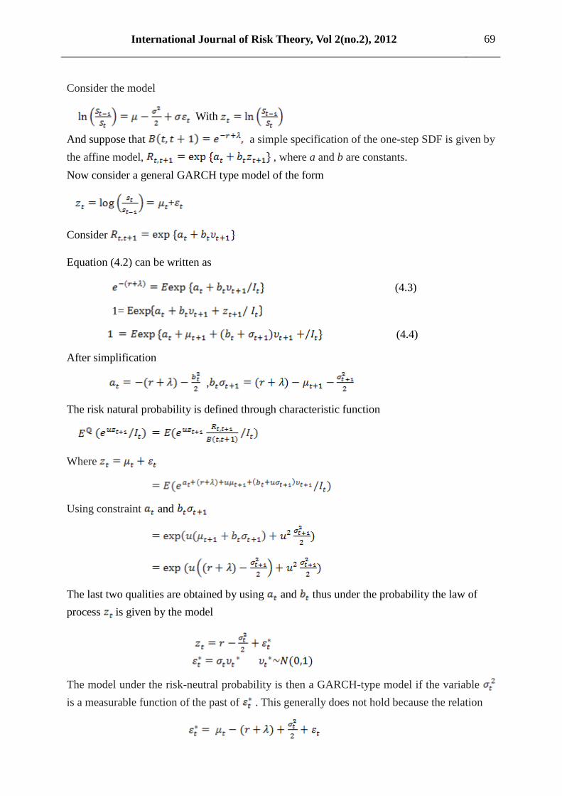
International Journal of Risk Theory, Vol 2(no.2), 2012 69
Consider the model
With
And suppose that a simple specification of the one-step SDF is given by
the affine model, , where a and b are constants.
Now consider a general GARCH type model of the form
+
Consider
Equation (4.2) can be written as
(4.3)
1=
(4.4)
After simplification
,
The risk natural probability is defined through characteristic function
Where
Using constraint and
The last two qualities are obtained by using and thus under the probability the law of
process is given by the model
The model under the risk-neutral probability is then a GARCH-type model if the variable
is a measurable function of the past of . This generally does not hold because the relation
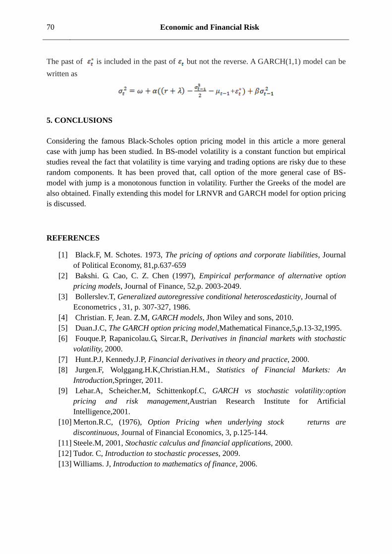
70 Economic and Financial Risk
The past of is included in the past of but not the reverse. A GARCH(1,1) model can be
written as
+
5. CONCLUSIONS
Considering the famous Black-Scholes option pricing model in this article a more general
case with jump has been studied. In BS-model volatility is a constant function but empirical
studies reveal the fact that volatility is time varying and trading options are risky due to these
random components. It has been proved that, call option of the more general case of BS-
model with jump is a monotonous function in volatility. Further the Greeks of the model are
also obtained. Finally extending this model for LRNVR and GARCH model for option pricing
is discussed.
REFERENCES
[1] Black.F, M. Schotes. 1973, The pricing of options and corporate liabilities, Journal
of Political Economy, 81,p.637-659
[2] Bakshi. G. Cao, C. Z. Chen (1997), Empirical performance of alternative option
pricing models, Journal of Finance, 52,p. 2003-2049.
[3] Bollerslev.T, Generalized autoregressive conditional heteroscedasticity, Journal of
Econometrics , 31, p. 307-327, 1986.
[4] Christian. F, Jean. Z.M, GARCH models, Jhon Wiley and sons, 2010.
[5] Duan.J.C, The GARCH option pricing model,Mathematical Finance,5,p.13-32,1995.
[6] Fouque.P, Rapanicolau.G, Sircar.R, Derivatives in financial markets with stochastic
volatility, 2000.
[7] Hunt.P.J, Kennedy.J.P, Financial derivatives in theory and practice, 2000.
[8] Jurgen.F, Wolggang.H.K,Christian.H.M., Statistics of Financial Markets: An
Introduction,Springer, 2011.
[9] Lehar.A, Scheicher.M, Schittenkopf.C, GARCH vs stochastic volatility:option
pricing and risk management,Austrian Research Institute for Artificial
Intelligence,2001.
[10] Merton.R.C, (1976), Option Pricing when underlying stock returns are
discontinuous, Journal of Financial Economics, 3, p.125-144.
[11] Steele.M, 2001, Stochastic calculus and financial applications, 2000.
[12] Tudor. C, Introduction to stochastic processes, 2009.
[13] Williams. J, Introduction to mathematics of finance, 2006.
International Journal of Risk Theory, Vol 2(no.2), 2012 71
ON CERTAIN FUNDAMENTAL PROPERTIES of HYPERGROUPS and
FUZZY HYPERGROUPS – MIMIC FUZZY HYPERGROUPS
Christos G. Massouros1, Gerasimos G. Massouros
1
1Technological Institute of Chalkis, GR34400, Evia, Greece
E-mail: [email protected]; [email protected]
ABSTRACT
In this paper, properties of hypergroups pertaining to the relationship between the hypercomposition and
induced hypercompositions with the empty set are presented. Analogous fuzzy hypergroup properties are also
proven. Finally, the study of these properties leads to the introduction of the mimic fuzzy hypergroup (fuzzyM -
hypergroup).
KEYWORDS
hypergroup, fuzzy hypergroup.
AMS
Classification number: 20N20
1. INTRODUCTION
Almost all fields of science desire to and attempt to utilize mathematical models in the
process of not only describing the various phenomena under study, but in also predicting,
wherever and whenever possible, the results generated through the influence of various
causes. Several of the mathematical models thus utilized are non-deterministic, as several
phenomena incorporate numerous uncertainties. Theory of probability, stochastic processes,
fuzzy set theory, soft set theory, vague set theory, hypercompositional algebra, etc., are all
different ways of expressing uncertainty. The self-contained development, as well as the
cross-linking of the above theories hold great attraction for mathematicians. For example, A.
Maturo, in a series of articles of his, (e.g. [39, 40, 41, 42] delved into linking the theory of
probability with hypercompositional algebra. On the other hand, several mathematicians
worked on linking fuzzy set theory with hypercompositional algebra.
One can distinguish three approaches, which were employed in order to connect these
two topics. One approach is to consider a certain hyperoperation defined through a fuzzy set
(P. Corsini [4], P. Corsini - V. Leoreanu, [6], I. Cristea e.g. [7, 8, 9], I. Cristea - S. Hoskova
[10], M. Stefanescu - I. Cristea [49], K. Serafimidis et al. [48] etc.). Another is to consider
fuzzy hyperstructures in a similar way as Rosenfeld did for fuzzy groups [46] (Zahedi, A.
72 Mathematics and Informatics for Risk Theory
Hasankhani [12, 54, 55], B. Davvaz [11] and others). The third approach is employed in the
pioneering papers by P. Corsini - I. Tofan [5] and by I. Tofan - A. C. Volf [50, 51], which
introduce fuzzy hyperoperations that induce fuzzy hypergroups. This approach was further
adopted by other researchers (Ath. Kehagias e.g. [15, 16, 17, 18], V. Leoreanu-Fotea e.g. [22,
23] etc.). M. K. Sen, R. Ameri and G. Chowdhury utilized this concept in defining fuzzy
hypersemigroups [47].
This paper deals with the algebra of hypergroups and fuzzy hypergroups. In researching
all relevant bibliography, we came to realize that there exists a certain amount of confusion in
some fundamental matters. For example, in attempting to define the hypergroup, some authors
view the hyperoperation on a non-void set H as a function from HH to the power set P(H)
of H, while others view it as a function from HH to P*(H), i.e. to the set of all non-empty
subsets of H. Certain fundamental properties of hypergroups and fuzzy hypergroups, which
are proven herein, afford us a clearer view of such matters.
2. ON CRISP HYPERCOMPOSITIONS
Hypercompositional algebra was born in 1934, when F. Marty, in order to study problems
in non-commutative algebra, such as cosets determined by non-invariant subgroups,
generalized the notion of the group, thus defining the hypergroup [24]. The hypergroup is an
algebraic structure in which the result of the composition of two elements is not an element
but a set of elements. To make this paper self-contained, we begin by listing some definitions
from the theory of hypercompositional structures (see also [35]). A (crisp) hypercomposition
or hyperoperation in a non-empty set H is a function from HH to the power set P(H) of H. A
non-void set H endowed with a hypercomposition “” is called hypergroupoid if ab for
any a,b in H, otherwise it is called partial hypergroupoid. Note that, if A, B are subsets of
H , then AB signifies the union a,b A B
ab
. Since AB= A= or B=, one can
observe that if A= or B=, then AB= and vice versa. aA and Aa have the same meaning
as a A and A a respectively. Generally, the singleton a is identified with its member
a .
A hypergroup is a non-void set H endowed with a hypercomposition which satisfies the
following axioms:
i. ab c a bc for every a,b,c H (associativity) and
ii. aH Ha H for every a H (reproduction).
If only (i) is valid, then the hypercompositional structure is called semi-hypergroup, while if
only (ii) is valid, then it is called quasi-hypergroup. The quasi-hypergroups in which the
weak associativity is valid, i.e. (ab)ca(bc) for every a,b,cH, were named HV-groups
[52].
Remark. If a non-void set H is endowed with a composition which satisfies the
International Journal of Risk Theory, Vol 2(no.2), 2012 73
associative and the reproduction axioms, then H is a group. Indeed let x H . Per
reproduction x xH . Therefore there exists e H such that xe x . Next let y be an
arbitrary element in H . Per reproduction there exists z H such that y zx . Consequently
ye zx e z xe zx y . Hence e is a right neutral element. Now, per reproduction
e xH . Thus there exists x H , such that e xx . Hence any element in H has a right
inverse.
Proposition 2.1. The result of the hypercomposition of any two elements in a hypergroup
is always non-void.
Proof. Let H be a hypergroup and suppose that ab= for some a,bH . Per
reproduction, aH=H and bH=H . Hence, H=aH=a(bH)=(ab)H=H= , which is
absurd.
Proposition 2.2. If the weak associativity is valid in a hypercompositional structure, then
the result of the hypercomposition of any two elements is always non-void.
Proof. Let H be a non-void set endowed with a hypercomposition satisfying the weak
associativity. Suppose that ab= for some a,bH. Then, (ab)c= for any cH .
Therefore, (ab)ca(bc)= , which is absurd. Hence, ab is non-void.
Corollary 2.1. The result of the hypercomposition of any two elements in a HV-group is
always a non-void set.
F. Marty also defined in [24] the two induced hypercompositions (right and left division)
resulting from the hypercomposition of the hypergroup, i.e.:
a
x H | a xbb
and
ax H | a bx
b
.
It is obvious that, if the hypergroup is commutative, then the two induced hypercompositions
coincide. For the sake of notational simplicity, a / b or a : b is used to denote the right
division (as well as the division in commutative hypergroups) and b\ a or a..b is used to
denote the left division. F. Marty's life was cut short, as he was killed during a military
mission in World War II. [24, 25, 26] are the only works on hypergroups he left behind.
However, several relevant papers by other authors began appearing shortly thereafter (e.g.
Krasner [19, 20], Kuntzmann [21] etc). Up to the present, a vast number of papers has been
produced on this subject (e.g.: see [3, 6])
In [13] and then in [14], a principle of duality is established in the theory of hypergroups.
More precisely, two statements of the theory of hypergroups are dual, if each results from the
other by interchanging the order of the hypercomposition, i.e. by interchanging any
hypercomposition ab with the hypercomposition ba . One can observe that the associativity
axiom is self-dual. The left and right divisions have dual definitions, thus they must be
interchanged in a construction of a dual statement. Therefore, the following principle of
duality holds true:
74 Mathematics and Informatics for Risk Theory
Given a theorem, the dual statement resulting from interchanging the order
of hypercomposition “” (and, by necessity, interchanging of the left and the
right divisions), is also a theorem.
This principle is used throughout this paper. The following properties are direct consequences
of the hypergroup axioms and the principle of duality is used in their proofs.
Proposition 2.3. a/b and b\a for all the elements a,b of a quasi-hypergroup H.
Proof. Per reproduction, Hb=H for every bH . Hence, for every aH there exists
xH , such that axb . Thus, xa/b and, therefore, a/b . Dually, b \a .
Proposition 2.4. In a quasi-hypergroup H, the non-empty result of the induced
hypercompositions is equivalent to the reproduction axiom.
Proof. Suppose that x/a for every a,xH . Thus, there exists yH , such that
xya . Therefore, xHa for every xH and so HHa . Next, since HaH for every aH ,
it follows that H=Ha . Per duality, H=aH . Conversely now, per Proposition 2.3, the
reproduction axiom implies that a/b and that a \b for every a,b in H.
Based on Proposition 2.4, we are now in a position to give an equivalent definition of the
hypergroup.
Definition 2.1. A hypergoup is a non-void (crisp) set H endowed with a (crisp)
hypercomposition, i.e. a function from H H to the powerset P H of H , which satisfies
the following axioms:
i. ab c a bc for every a,b,c H (associativity) and
ii. a/b and b\a for every a,b H .
Proposition 2.5. In a hypergroup H , equalities (i) H=H/a=a/H and (ii) H=a \H=H \a
are valid for every a in H.
Proof. (i) Per Proposition 2.1, the result of hypercomposition in H is always a non-
empty set. Thus, for every xH there exists yH , such that yxa , which implies that
xy/a . Hence, HH/a . Moreover, H/aH . Therefore, H=H/a . Next, let xH . Since
H=xH , there exists yH such that axy , which implies that xa/y . Hence, /H a H .
Moreover, /a H H . Therefore, H a / H . (ii) follows by duality.
The hypergroup is a very general structure, which was progressively enriched with
additional axioms, either more or less powerful. This created a significant number of specific
hypergroups. Moreover, some of these hypergroups constituted a constructive origin for the
development of other new hypercompositional structures (e.g.: see [3, 6, 27, 28, 29, 32, 34,
36, 43]). Thus, W. Prenowitz enriched hypergroups with an axiom, in order to utilize them in
the study of geometry [e.g.: see 44, 45]. More precisely, he introduced into the commutative
hypergroup the transposition axiom
a / b c / d implies ad bc for every a,b,c,d H
International Journal of Risk Theory, Vol 2(no.2), 2012 75
and named this new hypergroup join space [44]. For the sake of terminology unification, join
spaces are also called join hypergroups [30]. It has been proven that these hypergroups also
comprise a useful tool in the study of languages and automata [34, 37]. Later on, J. Jantosciak
generalized the above axiom in an arbitrary hypergroup as follows:
b\ a c / d implies ad bc for every a,b,c,d H .
He named this particular hypergroup transposition hypergroup [13]. Clearly, if A,B,C
and D are subsets of H , then B\ A C / D implies that AD BC . In [31, 38]
specialized transposition hypergroups were studied and, in [33], the transposition axiom was
introduced into ΗV-groups and the transposition ΗV-group was thus defined.
3. ON FUZZY HYPERCOMPOSITIONS
Zadeh, in 1965, in order to provide «a natural way of dealing with problems in which
the source of imprecision is the absence of sharply defined criteria of class membership,
rather than the presence of random variables» [53] introduced the notion of fuzzy sets. If H is
a non-void crisp set, then a fuzzy subset of H is a mapping from H to the interval of real
numbers [0,1]. If A H , then the characteristic function A of A
AX : H [0,1], 1
0
A
if x Ax X x
if x A
is a fuzzy subset of H . Thus, if A , then its characteristic function is the identically zero
function 0H , i.e. 0 0HX x x for every x H . Moreover, if A H , H , then
the characteristic function of the entire set H, is ( ) 1 ( ) 1H HX x x for every x H . Thus,
we can consider crisp sets as special case of fuzzy sets and identify every set (crisp or fuzzy)
with its membership function. The collection of all fuzzy subsets of H is denoted by F H .
A fuzzy hypercomposition maps the pairs of elements of the Cartesian product H H to fuzzy
subsets of H, i.e. : H H F H . Hence, if is a fuzzy hyperoperartion, then a b is a
function and the notation a b x means the value of a b at the element x. The definition
of the fuzzy hyperoperartion subsumes the relevant one of crisp hyperoperation as a special
case, since the later results from the former using the characteristic function.
Definition 3.1. [17, 18] If : HH F(H) is a fuzzy hypercomposition, then for every
aH, BF(H), the fuzzy sets a B and B a are defined respectively by
y Ha B z a y z B y
y HB a z y a z B y .
Per definition 3.1, if a,b,c H , then:
76 Mathematics and Informatics for Risk Theory
y Ha b c z a y z b c y
and y Ha b c z y c z a b y
Definition 3.2. [17, 18] If : HH F(H) is a fuzzy hypercomposition, then, for every
A,BF(H), the fuzzy set A B is defined by
x,y HA B z x y z A x B y .
As mentioned above, these definitions subsume the relevant ones of crisp hyperoperations as
special cases. For example, if AX is the characteristic function of the crisp set A, then, per
Definition 2.1:
A y H A Ay:z x yx X z x y z X y X y
.
Hence Ax X is the characteristic function of the crisp set y AxA xy (see also [17]).
Definition 3.3. If aH and A, BP(H), then Ba B a X , BB a X a and
A BA B X X .
Definition 3.4. [5, 51] If : HH F(H) is a fuzzy hypercomposition, then H is called
fuzzy hypergroup, if the following two axioms are valid:
i. a b c a b c for every a,b,c H (associativity),
ii. Ha H H a X for every a H (reproduction).
If (i) is only valid, then H is called a fuzzy semi-hypergroup [47] while if (ii) is only valid, then
H is called a fuzzy quasi-hypergroup.
Lemma 3.1. For every a, b H and C F(H), the following is true:
a b C a b C .
Proof. x,y Ha b C z y x z a b y C x =
x H y H y x z a b y C x =
x H x Ha b x z C x a b x z C x =
x H y H a y z b x y C x
x,y H a y z b x y C x
International Journal of Risk Theory, Vol 2(no.2), 2012 77
y H x Ha y z b x y C x
y H a y z b C y a b C z .
Proposition 3.1. 0Ha b is valid for any pair of elements a, b in a fuzzy hypergroup H.
Proof. Suppose that 0Ha b for some a,bH . Per reproduction, Ha H X and
Hb H X . Hence, HX a H a b H . Per Lemma 3.1, the equality
a b H a b H is valid. Since 0Ha b , we have: 0H Ha b H X . But
0 0 0H H x,y H H H HX z x y z x X y z . Therefore, 0H HX ,
which is absurd because H .
The fuzzy HV-groups were defined in [15]. If A, BF(H) and 0,1p , then we write
pA B , if there exists x H such that A x B x p . The fuzzy quasi-hypergroups in
which the weak associativity is valid, i.e. pa b c a b c for every a,b,cH, are named
fuzzy HV-groups.
Proposition 3.2. If a fuzzy hypercompositional structure ,H is endowed with the weak
associativity, then 0Ha b is valid for every ,a b H .
Proof. Suppose that 0Ha b for some a,bH . Then 0Ha b c c , for any
cH . Since 0 0 0H y H Hc z y c z y , it follows that 0 0H Hc and,
therefore, 0Ha b c . Hence, the weak associativity is not valid in ,H , which
contradicts our supposition.
Corollary 3.1. The result of the hypercomposition of any two elements in a fuzzy HV-
group is always a non-zero function.
4. THE MIMIC FUZZY HYPERGROUP
If H is a non-void set endowed with a fuzzy hypercomposition , then two new induced
fuzzy hypercompositions “/” and “\” can be defined as follows:
/a b x x b a for every , ,a b x H and
\b a x b x a for every , ,a b x H .
As in the case of crisp hypercompositions, the two induced fuzzy hypercompositions will
be called fuzzy right division and fuzzy left division respectively (see also [2]).
78 Mathematics and Informatics for Risk Theory
Proposition 4.1. For any pair of elements a,b in a fuzzy hypergroup H, 0Ha / b and
0Ha\b is valid.
Proof. Per reproduction, HH b X is valid for every bH . Thus, equality
HH b a X a is true for any aH . Since
y H HH b a y b a X y ,
it follows that there exists yH such that 1y b a or, equivalently, 1a / b y .
Therefore, 0Ha / b . Dually, 0Ha\b .
It becomes obvious that a statement analogous to Proposition 2.4 is not valid in the case
of fuzzy hypergroups. Indeed:
Example 4.1. Let H a,b and suppose that
a a a a a b a b a b b a
and a a b a b b b a a b a b b b a b b b
Then, H , is a fuzzy semi-hypergroup. Suppose that 0x y z for every , ,x y z H .
Then, in this fuzzy semi-hypergroup, 0Ha / b and 0Ha\b is valid for every ,a b H .
Yet, if 1x y z for any , ,x y z H , one can easily see that the reproduction is not
verified.
These ideas lead to the introduction of the following definition:
Definition 4.1. If : HH F(H) is a fuzzy hypercomposition, then H is called mimic
fuzzy hypergroup (fuzzyM-hypergroup), if the following two axioms are valid:
i. a b c a b c for every a,b,c H (associativity),
ii. 0Ha / b and 0Ha\b for every a,b H .
If (ii) is only valid, then H is called mimic fuzzy quasi-hypergroup (fuzzyM-quasi-hypergroup)
while, if instead of (i) the weak associativity is valid, then H is called mimic fuzzy Hv- group
(fuzzyM Hv-group).
Proposition 4.2. In a fuzzyM-hypergroup H , it holds that 0H a x and
0a H x for every a,xH.
Proof. Since 0Hx / a for every a,x H , it follows that there exists yH such that
0x / a y . Hence, there exists yH such that 0y a x , for any a,x H . Since
International Journal of Risk Theory, Vol 2(no.2), 2012 79
y H HH a x y a x X y , it follows that 0H a x for every a,x H .
Per duality, 0a H x for every a,x H .
Proposition 4.3. In a fuzzyM-hypergroup H , it holds that 0Ha b for every a,bH.
Proof. Suppose that there are a,b H such that 0Ha b . Then 0Ha b H . Per
Lemma 3.1, a b H a b H . Hence 0Ha b H . But
y Ha b H z a y z b H y
Per Proposition 4.2, 0b H y , for every b,yH. Therefore 0a y z for every
z,yH. Thus 0a\ z y for every y H , which is absurd.
It is obvious that if a fuzzyM-hypergroup H is commutative, then a H H a for any
a H . However, generally speaking, this equality is not valid. Hence, we have the
following definition:
Definition 4.2. A fuzzyM-hypergroup H will be called commutable fuzzyM-hypergroup, if
a H H a for any a H .
Example 4.2. Let H a,b and suppose that:
0 1 0 2
0 2 0 5
0 7 0 9
a a a , ; a a b ,
b a a a b b b a b , ; a b a ,
b b a , ; b b b ,
Then H , is a non-commutative fuzzyM-hypergroup, since a b a b a a .
Furthermore H , is non-commutable. Next if we define:
0 1
0 9
a a b b a a ,
a a a b b a b b b a b a a b b b a b ,
then H , is a non-commutative fuzzyM-hypergroup, since a b a b a a .
However H , is commutable. Moreover if we define:
0 1
0 2
a a a b b a a b a b a a ,
a a b b b b a b b b a b ,
then H , is a commutative fuzzyM-hypergroup.
As in the case of fuzzy hypergroups [1, 2, 15, 16], the transposition axiom can be
80 Mathematics and Informatics for Risk Theory
introduced in fuzzyM-hypergroups as well. Thus, we have the definition:
Definition 4.3. A fuzzyM-hypergroup H will be called transposition fuzzyM-hypergroup, if
for any a, b, c, d H for which there exists 0,1p such that pb\ a c / d , there exists
also 0,1q such that qa d b c . If p q for every a, b, c, d H, then H will be
called p-transposition fuzzyM-hypergroup.
REFERENCES
[1] R. Ameri, Fuzzy transposition hypergroups, Ital. J. Pure Appl. Math. No. 18, 167-174,
2005
[2] G. Chowdhury, Fuzzy transposition hypergroups, Iranian Journal of Fuzzy Systems Vol.
6, No. 3, pp. 37-52, 2009
[3] P. Corsini, Prolegomena of hypergroup theory, Aviani Editore, 1993.
[4] P. Corsini, Join spaces, power sets, fuzzy sets, Algebraic Hyperstructures and
Applications, ed. M. Stefanescu, Hadronic Press, pp. 45-52, 1994.
[5] P. Corsini, I. Tofan, On fuzzy hypergroups. Pure Math Appl 8, pp. 29-37, 1997.
[6] P. Corsini, V. Leoreanu, Applications of Hyperstructures Theory, Kluwer Academic
Publishers, 2003.
[7] I. Cristea, Hyperstructures and fuzzy sets endowed with two membership functions,
Fuzzy Sets and Systems 160 (8), 1114-1124, 2009.
[8] I. Cristea, About the fuzzy grade of the direct product of two hypergroupoids, Iran. J.
Fuzzy Syst. 7, No. 2, 95-108, 2010
[9] I. Cristea, On the Fuzzy Subhypergroups of Some Particular Complete Hypergroups (I),
World Applied Sciences Journal 7 pp. 57-63, 2009
[10] I. Cristea, S. Hoskova, Fuzzy Pseudotopological Hypergroupoids, Iranian Journal of
Fuzzy Systems Vol. 6, No. 4, pp. 11-19, 2009.
[11] B. Davvaz, Fuzzy HV –groups, Fuzzy Sets and Systems 101, 191-195, 1999
[12] A. Hasankhani, M.M. Zahedi, Fuzzy sub-F-polygroups, Ratio Mathematica 12, pp. 35-
44, 1997.
[13] J. Jantosciak, Transposition hypergroups, Noncommutative Join Spaces, Journal of
Algebra, 187, pp. 97-119, 1997.
[14] J. Jantosciak, Ch. G. Massouros, Strong Identities and fortification in Transposition
hypergroups, Journal of Discrete Mathematical Sciences & Cryptography 6, no 2-3, pp.
169-193, 2003.
[15] Ath. Kehagias, An example of L-fuzzy Join Space, Rendiconti del Circolo Matematico del
Palermo, vol.51, pp.503-526, 2002.
[16] Ath. Kehagias, L-fuzzy Meet and Join Hyperoperations, Proc. of 8th Conference on
Algebraic Hyperstructures and Applications, Samothraki, 2002.
[17] Ath. Kehagias, K. Serafimidis, The L-Fuzzy Nakano Hypergroup, Information Sciences,
vol. 169, pp.305-327, 2005.
[18] Ath. Kehagias, The Construction of Fuzzy-valued t-norms and t-conorms, Studies in
Computational Intelligence (SCI) 67, pp. 361-370, 2007.
International Journal of Risk Theory, Vol 2(no.2), 2012 81
[19] M. Krasner, La loi de Jordan - Holder dans les hypergroupes et les suites generatrices
des corps de nombres P - adiqes. (I) Duke Math. J. 6, pp. 120-140, 1940, (II) Duke
Math. J. 7, pp. 121-135, 1940.
[20] M. Krasner, La characterisation de hypergroupes de classes et le probleme de Schreier
dans ces hypergroupes, C. R. Acad. Sci. (Paris), 212, 1941, pp. 948-950, 218, pp. 483-
484 et pp. 542-544, 1944.
[21] J. Kuntzmann, Opérations multiformes. Hypergroupes, Comptes Rendus Acad. Sci., vol
204, pp. 1787-1788 (Paris, 1937)
[22] V. Leoreanu, About hyperstructures associated with fuzzy sets of type 2, Italian J. of Pure
and Appl. Math., 17, 127-136, 2005.
[23] V. Leoreanu-Fotea, Fuzzy join n-ary spaces and fuzzy canonical n-ary hypergroups,
Fuzzy Sets and Systems 161, pp. 3166–3173, 2010.
[24] F. Marty, Sur un généralisation de la notion de groupe. Huitième Congrès des
mathématiciens Scand., Stockholm 1934, pp. 45-49.
[25] F. Marty, Rôle de la notion de hypergroupe dans l' étude de groupes non abéliens, C.R.
Acad. Sci. (Paris) 201, pp. 636-638, 1935.
[26] F. Marty, Sur les groupes et hypergroupes attachés à une fraction rationelle, Annales de
l’ école normale, 3 sér., vol. 53, pp. 83-123, 1936.
[27] Ch. G. Massouros, On the theory of hyperrings and hyperfields, Algebra i Logika 24,
No 6, pp. 728-742, 1985.
[28] Ch. G. Massouros, Free and cyclic hypermodules, Annali Di Mathematica Pura ed
Applicata, Vol. CL. pp. 153-166, 1988.
[29] Ch. G. Massouros, On the Hypercompositional Structures, Fuzzy Systems & A.I.-
Reports and Letters, Academia Romana, Vol. 3, no. 3, pp. 15-27, 1994.
[30] Ch. G. Massouros, Canonical and Join Hypergroups, An. Stiintifice Univ. "Al. I. Cuza",
Iasi, Tom. XLII, Matematica, fasc.1, pp. 175-186, 1996.
[31] Ch. G. Massouros, G. G. Massouros, Transposition Polysymmetrical Hypergroups with
Strong Identity, Journal of Basic Science Vol. 4, No. 1, pp. 85-93, 2008.
[32] Ch. G. Massouros, G. G. Massouros, On Join Hyperrings. Proceedings of the 10th
Internat. Cong. on Algebraic Hyperstructures and Applications. pp. 203-216, Brno,
Czech Republic 2008
[33] Ch. G. Massouros, A. Dramalidis, Transposition Hv-groups, Ars Combinatoria, Vol. 105,
2012.
[34] G. G. Massouros, Automata and Hypermoduloids, Proceedings of the 5th Internat. Cong.
on Algebraic Hyperstructures and Applications, pp. 251-266, Iasi 1993, Hadronic Press
1994.
[35] G. G. Massouros, On the Hypergroup Theory, Fuzzy Systems & A.I. - Reports and
Letters, Academia Romana, IV, no. 2/3, pp. 13-25, 1995.
[36] G. G. Massouros, The Hyperringoid, Multiple Valued Logic, Vol. 3, pp. 217-234, 1998.
[37] G. G. Massouros, Hypercompositional Structures from the Computer Theory, Ratio
Matematica, no 13, pp. 37-42, 1999.
[38] G. G. Massouros, F. A. Zafiropoulos and Ch. G. Massouros, Transposition
Polysymmetrical Hypergroups, Proceedings of the 8th Internat. Cong. on Algebraic
Hyperstructures and Applications, Samothraki 2002, Spanidis Press 2003, pp. 191-202.
[39] A. Maturo, Conditional events, conditional probabilities and hyperstructures, in
Proceedings EUFIT ’97, September 8-11, 1997, pp. 1509/1513, Aachen, Germany
[40] A. Maturo, On a non-standard algebraic hyperstructure and its applications to the
coherent probability assessments, Italian Journal of Pure and Applied Mathematics, n. 7,
pp. 33-50, 2000.
82 Mathematics and Informatics for Risk Theory
[41] A. Maturo, Finitely additive conditional probability with value on a hyperstructure, J. of
Information & Optimization Sciences ,vol. 22, 1, 2001
[42] A. Maturo, Hypergroups and Generalized probabilities, Advances in Generalized
Structures, Approssimate Reasoning and Applications, pp. 13-29, Performantica Press,
Iasi, Romania, 2001
[43] J. Mittas, Sur certaines classes de structures hypercompositionnelles. Proceedings of the
Academy of Athens, Vol. 48, pp. 298 - 318, Athens 1973.
[44] W. Prenowitz, A Contemporary Approach to Classical Geometry, Amer. Math. Month.
vol. 68, no 1, part II, pp. 1-67, 1961.
[45] W. Prenowitz, J. Jantosciak, Geometries and Join Spaces. J. Reine Angew. Math. 257, pp.
100-128, 1972.
[46] A. Rosenfeld, Fuzzy Groups, J. Math. Anal. Appl. 35, pp. 512-517, 1971.
[47] M. K. Sen, R. Ameri, G. Chowdhury, Fuzzy hypersemigroups, Soft Comput. 12 pp. 891-
900, 2008.
[48] K. Serafimidis, Ath. Kehagias, M. Konstantinidou, The L-Fuzzy Corsini Join
Hyperoperation, Italian Journal of Pure and Applied Mathematics, vol.12, pp.83-90,
2002.
[49] M. Stefanescu, I. Cristea, On the fuzzy grade of hypergroups, Fuzzy Sets and Systems
159 (9), pp. 1097-1106, 2008.
[50] I. Tofan, A. C. Volf, On some connections between hyperstructures and fuzzy sets, Italian
J. of Pure and Appl. Math., 7, 63-68, 2000.
[51] I. Tofan, A. C. Volf, Algebraic aspects of information organization, Systematic
Organisation of Information in Fuzzy Systems, P. Melo-Pinto et al. (Eds) IOS Press, pp.
71-87, 2003.
[52] T. Vougiouklis, The fundamental relation in hyperrings. The general hyperfield. Proc. of
the 4th AHA, Xanthi, Greece 1990, World Scientific 1991, pp. 209-217.
[53] L. A. Zadeh, Fuzzy sets, Inform. Control, 8, 338-353, 1965.
[54] M. M. Zahedi, A. Hasankhani, F-Polygroups, Int. J. Fuzzy Math., vol. 4, pp.533 -548,
1996.
[55] M. M. Zahedi, A. Hasankhani, F-Polygroups (II), Inf. Sciences, vol.89, pp.225-243,
1996.
International Journal of Risk Theory, Vol 2(no.2), 2012 83
AUTHOR GUIDELINES
JOURNAL TOPICS
Technological Risk
Economic and Financial Risk
Chemistry and Physics of Undesired Events
Mathematics and Informatics for Risk Theory
Natural Risk
PAPER FORMAT
Content will be in English, in doc format (for Microsoft Word), and the following format of
paragraph will be used: Identation: left 0, right 0; Spacing: before 0, after 0; Line spacing:
Multiple At 1.15.
Paper Title
Paper title will be written in 12-point bold type, Times New Roman in uppercase and will be
centered across the top of the page.
Paper Authors
Author's names will be written under the paper title, centered across the page, in 12 point
type, Times New Roman in lowercase.
Author's Affiliation
Author's affiliation will be written under the author's names, centered across the page, in 12
point type italic, Times New Roman in lowercase, specifying: title, university affiliation,
country and e-mail address.
Paper Abstract
The abstract must include sufficient information for readers to judge the nature and
significance of the topic, the adequacy of the investigative strategy, the nature of the results
and the conclusions. An abstract is not an introduction, it summarizes the substantive results
of the work, not merely list topics that are discussed in the paper.
The abstract will be written in 10 point type italic, Times New Roman. It must have 200 to
300 words, single spaced type.
84 Author Guidelines
Keywords
Select four to eight keywords (words or expressions) that capture the essence of your paper.
List the words in decreasing order of importance.
Introduction
The function of the Introduction is to establish the context of the paper. This is accomplished
by discussing the relevant primary research literature (with quotations) and summarizing
current understanding of the problem you are investigating. State the purpose of the work in
the form of the hypothesis, questions or problems you investigate and, briefly explain your
approach and the necessary arguments. Whenever possible, present the possible outcomes
your study can reveal.
Paper Body
Organize the body of the paper using titles and subtitles to emphasize both content and clarity.
Consider the following: use the accepted terminology of the field to describe any subjects or
experimental procedures used to gather and analyze data; include detailed methods, so readers
could be able to follow the investigation; state the results clearly and succinctly; thoroughly
discuss, interpret and analyze the implications of the findings and minutely discuss the impact
of the results, both globally and specifically.
The section titles will be written in 12-point bold type, Times New Roman in uppercase and
will be aligned to left. Typeface must be 12-point Times New Roman type single spaced.
Tables and figures should be sized and placed in the body of the paper just as the authors want
them printed in the journal. Care should be taken so that tables and figures could be on one
page. The tables contents will be written in 10 point type, Times New Roman and the heading
of the tables will be in 10 point type bold, Times New Roman. The titles and numbers will be
positioned above the table and the title and number of the figures bellow. When it is needed,
the source will be mentioned. The number of the tables and figures are to be positioned in the
body of the text, in a parenthesis, wherever they are mentioned, for example: (fig. nr.1), (table
nr. 1). The graphs must be executed clearly so as to give clear black and white copies. Number
all the equations and formulas used positioning the numbers in parenthesis on their right side.
Define abbreviations and acronyms the first time they are used in the text, even after they had
already been defined in the abstract. Avoid the use of footnotes or endnotes.
Conclusions
A conclusion section is required. Conclusions may review the main points of the paper, do not
replicate the abstract as the conclusion. A conclusion might elaborate on the importance of the
work or suggest applications and extensions and extensions of the research.

International Journal of Risk Theory, Vol 2(no.2), 2012 85
References
References will be written in the format of the following model:
[1] A. Edalat, M.B. Smyth, Information categories, Applied Categorical Structures, 1, 1993,
p. 197–232.
Also, references in the articles will be numbered with [1] and if there are more than one
reference with, [1,3] or [1-5]. Sources should be in alphabetical order by author’s last name.
When certain studies, research, articles are published in a volume, the volume numbers and
pages will be specified.
Recommended