Generalized acoustic energy density
Buye Xu,a) Scott D. Sommerfeldt, and Timothy W. LeishmanDepartment of Physics and Astronomy, Brigham Young University, Provo, Utah 84602
(Received 15 September 2010; revised 8 July 2011; accepted 21 July 2011)
The properties of acoustic kinetic energy density and total energy density of sound fields in lightly
damped enclosures have been explored thoroughly in the literature. Their increased spatial uniform-
ity makes them more favorable measurement quantities for various applications than acoustic
potential energy density (or squared pressure), which is most often used. In this paper, a generalized
acoustic energy density (GED), will be introduced. It is defined by introducing weighting factors
into the formulation of total acoustic energy density. With an additional degree of freedom, the
GED can conform to the traditional acoustic energy density quantities, or it can be optimized for
different applications. The properties of the GED will be explored in this paper for individual room
modes, a diffuse sound field, and a sound field below the Schroeder frequency.VC 2011 Acoustical Society of America. [DOI: 10.1121/1.3624482]
PACS number(s): 43.55.Br, 43.20.Ye, 43.55.Cs, 43.50.Ki [SFW] Pages: 1370–1380
I. INTRODUCTION
Since the pioneering work by Sabine,1 measurements
based on acoustic pressure, squared pressure, or acoustic
potential energy density have become a primary focus for
room acoustics. In the early 1930s, Wolff experimentally
studied the kinetic energy density as well as total energy
density in a room with the use of pressure gradient micro-
phones.2,3 His results indicated a better spatial uniformity of
both the kinetic energy density and total energy density over
the potential energy density.
In 1974, the preliminary experimental study by Sep-
meyer et al.4 showed that for a pure-tone diffuse sound field,
the potential energy density has a relative spatial variance of
1, which is consistent with the theoretical results by Water-
house5 and Lyon.6 In addition, they also found that the var-
iance of potential energy density is approximately twice that
of the total energy density. In the same year, Cook et al.showed that the spatial variance of total energy density is
smaller than that of the squared pressure for standing waves.7
Following Waterhouse’s free-wave concept,8,9 Jacobsen
studied the statistics of acoustic energy density quantities
from a stochastic point of view.10 Moryl et al.11,12 experi-
mentally investigated the relative spatial standard deviation
of acoustic energy densities in a pure tone reverberant field
with a four-microphone probe. Their results are in fair agree-
ment with Jacobsen’s prediction.
Jacobsen, together with Molares, revised his 1979
results10 by applying the weak Anderson localization argu-
ments,13 and they were able to extend the free-wave model to
low frequencies.14,15 The new formulas for sound power radi-
ation variance and ensemble variance of pure-tone excitations
are very similar to those derived from the modal model,6,16,17
but with a simpler derivation. The same authors then investi-
gated the statistical properties of kinetic energy density and
total acoustic energy density in the low frequency range.18
The pressure microphone gradient technique for meas-
uring acoustic energy quantities has been studied and
improved over time.3,4,11,19–22 Recently, a novel particle ve-
locity measurement device, Microflown, has been made avail-
able to acousticians,23,24 expanding the methods available to
measure acoustic energy density quantities. More and more
attention is consequently being devoted to their study and use.
By recognizing the increased uniformity of the total
energy density field, Parkins et al. implemented active noise
control (ANC) by minimizing the total energy density in
enclosures. Significant attenuation was achieved at low fre-
quencies.25,26 In 2007, Nutter et al. investigated acoustic
energy density quantities for several key applications in
reverberation chambers and explored the benefits introduced
by the uniformity of both kinetic energy density and total
acoustic energy density.27
Most studies of kinetic energy density and total energy
density have focused on their improved uniformity in rever-
berant sound fields. A new energy density quantity, the gen-
eralized acoustic energy density (GED), will be introduced
in this paper and shown to be more uniform than all other
commonly used acoustic energy density quantities. Yet it
requires no more effort to obtain than kinetic energy and
total energy density.
The paper will be organized as follows. The GED and
some of its general properties will be introduced in Sec. II.
In Sec. III its behavior will be explored for room modes. Its
properties in a diffuse field will be investigated in Sec. IV
with a focus on single-tone excitation and certain character-
istics of narrow-band excitation. In Sec. V its spatial var-
iance will be studied for frequencies below the Schroeder
frequency of a room. Computer simulation results will be
presented in Sec. VI to validate some of the GED properties
introduced in the paper. In Sec. VII three applications of the
GED will be studied experimentally and numerically.
II. GENERALIZED ENERGY DENSITY
The total acoustic energy density is defined as the acous-
tic energy per unit volume at a point in a sound field. The
a)Author to whom correspondence should be addressed. Electronic mail:
1370 J. Acoust. Soc. Am. 130 (3), September 2011 0001-4966/2011/130(3)/1370/11/$30.00 VC 2011 Acoustical Society of America
Redistribution subject to ASA license or copyright; see http://acousticalsociety.org/content/terms. Download to IP: 128.187.97.22 On: Thu, 13 Mar 2014 23:07:28
time-averaged total acoustic energy density can be expressed
in the frequency domain as
ET ¼ EP þ EK
¼ 1
2
pp�
q0c2þ 1
2q0u � u�; (1)
where p and u represent the complex acoustic pressure and
particle velocity, respectively, in the frequency domain, q0 is
the ambient fluid density, and c is the speed of sound. On the
right-hand side of this expression, the first term represents
the time-averaged potential energy density (EP) and the sec-
ond term represents the time-averaged kinetic energy density
(EK). The time-averaged kinetic energy density can be writ-
ten as the sum of three orthogonal components as
EK ¼ EKx þ EKy þ EKz
¼ 1
2q0uxu�x þ
1
2q0uyu�y þ
1
2q0uzu
�z : (2)
The GED is defined as follows:
EGðaÞ ¼ aEP þ ð1� aÞEK; (3)
where a is an arbitrary real number. The GED is simply the
sum of EP and EK with weighting factors that add to 1. One
can cause the GED to represent the traditional energy density
quantities by appropriately varying a. In other words, EP
¼ EGð1Þ, EK ¼ EGð0Þ, and ET ¼ 2EGð1=2Þ. Although, in theory,
a could be any real number, the range 0 � a � 1 will be the
focus of this work, because it contains all values of a that
make GED favorable for the applications studied herein.
However, most theoretical derivations presented in this paper
are general enough that the results can be implemented
directly for the entire domain of real numbers.
The spatial mean of GED for a sound field can be calcu-
lated as
lG ¼ E½EG� ¼ E½aEP þ ð1� aÞEK �¼ alP þ ð1� aÞlK; (4)
where E½� � �� represents the expectation operator and lG, lP,
and lK represent the spatial mean value of EG, EP, and EK ,
respectively. Given that lP ¼ lK for most enclosed sound
fields,10 one can conclude from Eq. (4) that lG does not vary
due to a, and lG ¼ lP ¼ lK .
The relative spatial variance of GED can similarly be
calculated as
�2G ¼
r2 EG½ �E2 EG½ �
¼ E½E2G��E2½EG�E2½EG�
¼ a2E½E2P�þ 2að1� aÞE½EPEK�þ ð1� aÞ2E½E2
K��l2G
l2G
¼ a2ðE½E2P��l2
PÞl2
P
þð1� aÞ2ðE½E2K��l2
KÞl2
K
þ 2að1� aÞðE½EPEK� �lPlKÞlPlK
¼ a2�2Pþð1� aÞ2�2
K þ 2að1� aÞ�2PK; (5a)
¼ a2ð�2P þ �2
K � 2�2PKÞ þ 2að�2
PK � �2KÞ þ �2
K; (5b)
where r2 � � �½ � represents the spatial variance; �2G, �2
P, and �2K
represent the relative spatial variances of EG, EP, and EK
respectively; and �2PK represents the relative spatial co-var-
iance of EP and EK . In the derivation of the equations above,
the relations of lG ¼ alP þ ð1� aÞlK and lG ¼ lP ¼ lK
are utilized. One can show by substituting appropriate values
for a that Eq. (5a) can revert to �P (a ¼ 1) and �K (a ¼ 0).
Equation (5b) shows that the relative variance of GED is a
quadratic function of a. In addition, recognizing that
�2P þ �2
K > 2�2PK , one can conclude that �2
G has a global
minimum,
minf�2Gg ¼
�2P�
2K � �4
PK
ð�2P þ �2
K � 2�2PKÞ
; (6)
when
a ¼ ð�2K � �2
PKÞð�2
P þ �2K � 2�2
PKÞ: (7)
As explained in the following discussion, the kinetic energy
density and total energy density may not be the most spa-
tially uniform quantities.
III. MODAL ANALYSIS
Below the Schroeder frequency, distinct room modes of-
ten dominate an enclosed sound field. Consider a hard-
walled rectangular room with dimensions Lx � Ly � Lz, with
a single mode dominating the response at a resonance fre-
quency. Ignoring any constants, EP and EK can be expressed
approximately as28
EP ¼ cos2ðkxxÞ cos2ðkyyÞ cos2ðkzzÞ;
EK ¼k2
x sin2ðkxxÞ cos2ðkyyÞ cos2ðkzzÞk2
(8a)
þk2
y cos2ðkxxÞ sin2ðkyyÞ cos2ðkzzÞk2
þ k2z cos2ðkxxÞ cos2ðkyyÞ sin2ðkzzÞ
k2; (8b)
where kx, ky, and kz are eigenvalues and k2 ¼ k2x þ k2
y þ k2z .
For an axial mode, where two of the three eigenvalues
vanish (assumed here in the y and z directions),
EG ¼ a cos2ðkxÞ þ ð1� aÞ sin2ðkxÞ;
�2G ¼ 2a2 � 2aþ 1
2: (9)
With no surprise, the relative variance reaches its minimum
value of zero when a ¼ 1=2, which corresponds to the total
acoustic energy density being uniform for an axial mode.
For a tangential mode (only 1 eigenvalue equals zero),
the expression for the relative variance is not as simple as
that for an axial mode. It depends on both a and the ratio
J. Acoust. Soc. Am., Vol. 130, No. 3, September 2011 Xu et al.: Generalized acoustic energy density 1371
Redistribution subject to ASA license or copyright; see http://acousticalsociety.org/content/terms. Download to IP: 128.187.97.22 On: Thu, 13 Mar 2014 23:07:28

c ¼ ky=kx (assuming kz ¼ 0), as shown in Table I. Some
examples of the spatial variance for different c values are
shown in Fig. 1(a). By assuming kx � ky, it is not difficult to
prove that �2G increases with c for all a values less than 1,
and as c tends to infinity, �2G converges to
�2G
��c!1¼
5
4� 3aþ 3a2: (10)
The optimized value of a, which minimizes the relative var-
iance, ranges between 1=4, when c ¼ 1, and 1=2, when
c!1. With the optimal a value, the relative variance can
become a tenth that of EP and half that of ET .
For an oblique mode, the relative variance again
depends on a as well as all the eigenvalues. With ratios
cxy ¼ ky=kx and cyz ¼ kz=ky, one can derive the expression
for �2G shown in Table I. When cxy approaches infinity while
cyz remains finite, the behavior of �2G is very similar to that of
the tangential modes. As a limiting case, when cxy !1 and
cyz ¼ 1, �2G converges to
�2G
��cxy!1;cyz¼1
¼ 7
8� 3a
2þ 3a2; (11)
which, similar to the tangential mode with c ¼ 1, reaches the
minimum when a ¼ 1=4. As the value cyz approaches infin-
ity, �2G converges to
�2G
��cyz!1
¼ 19
8� 9a
2þ 9a2
2; (12)
regardless of the value of cxy [see Fig. 1(b)]. The optimal avalue varies from 1=10 to 1=2 depending on the values of cxy
and cyz. However, as can be observed from Fig. 1(c), if
cyz < 2 the optimal a value is generally in the range of 0:1 to
0:35. With the optimal a value, the relative variance can
become a factor of 6:8 smaller than that of EP and half that
of ET . It is interesting to note that for all possible values of c,
cxy, and cyz, EP has the highest relative variance, which is a
constant for each type of mode.
IV. GED IN DIFFUSE FIELDS
The free-wave model5 has been successfully used to study
the statistical properties of diffuse sound fields. It assumes that
TABLE I. Relative variance of single modes.
Mode l �2P �2
G
Axial 1=2 1=2 ð2a� 1Þ2
2Tangential 1=4 5=4 5� 6c2 þ 5c4 � 4 3� 2c2 þ 3c4ð Þaþ 4 3þ 2c2 þ 3c4ð Þa2
4 1þ c2ð Þ2
Oblique 1=8 19=8 19� 10c2xyð1þ c2
yzÞ þ c4xyð19� 10c2
yz þ 19c4yzÞ
8 1þ c2xy þ c2
xyr22
� �2
�½3� 2c2
xyð1þ c2yzÞ þ c4
xyð3� 2c2yz þ 3c4
yz�a
2 1þ c2xy þ c2
xyr22
� �2
þ½3þ 2c2
xyð1þ c2yzÞ þ c4
xyð3þ 2c2yz þ 3c4
yz�a2
2 1þ c2xy þ c2
xyr22
� �2
FIG. 1. (Color online) Relative spatial variance of GED for (a) a tangential
mode and (b) an oblique mode. The contour plot (c) shows the optimal val-
ues of a that minimize �2G for the oblique modes.
1372 J. Acoust. Soc. Am., Vol. 130, No. 3, September 2011 Xu et al.: Generalized acoustic energy density
Redistribution subject to ASA license or copyright; see http://acousticalsociety.org/content/terms. Download to IP: 128.187.97.22 On: Thu, 13 Mar 2014 23:07:28

the sound field at any arbitrary point is composed of a large
number of plane waves with random phases and directions.
For a single-tone field, the complex acoustic pressure ampli-
tude for a given frequency can thus be written as
p ¼X
m
Ameiðknm�rþ/mÞ; (13)
where Am is a random real number representing the peak am-
plitude of the mth wave, and the unit vector nm and phase /m
are uniformly distributed in their spans.
It can be shown, based on the central limit theorem, that
the rms value of squared pressure has an exponential distribu-
tion,5,10 and the probability density function (PDF) of Ep is
fEPðxÞ ¼ 1
lG
e�x=lG ; x � 0: (14)
The mean and variance are lG and l2G, respectively, for the
exponentially distributed EP, so the relative variance is 1.
Using a similar argument, Jacobsen was able to show
that the three components of kinetic energy density (EKx,
EKy, and EKz) are independent and follow an exponential dis-
tribution. Therefore, the kinetic energy density is distributed
as Cð3; lG=3Þ,10 and the PDF is
fEKðxÞ ¼ 27x2e�3x=lG
2l3G
; x > 0: (15)
The mean and variance for this distribution are lG and l2G=3,
respectively, and the relative variance is 1=3, which is signif-
icantly less than that of the potential energy density.
Because EP and EK are independent,10 one can compute
the cumulative distribution function (CDF) and PDF for the
GED with the following equations:
FEGðxÞ ¼
ðx=a
0
fEPðyÞð x�ayð Þ= 1�að Þ
0
fEKðzÞdzdy; (16)
fEGðxÞ ¼ dFEG
ðxÞdx
: (17)
The calculation is rather involved, so only the final result for
the PDF will be shown here:
fEGðxÞ ¼27a2 e�3x=lGð1�aÞ � e�x=ðlGaÞ� �
lGð1� 4aÞ3
þ 27x xð1� 4aÞ � 2lGað1� aÞ½ �e�3x=lGð1�aÞ
2l3Gð1� aÞ2ð1� 4aÞ2
: (18)
It is not hard to show that Eq. (18) converges to Eq. (14) and
Eq. (15) for the limiting cases wherein a! 1 and a! 0,
respectively.
With the use of Eq. (18) [or Eq. (5a)], one can obtain
the relative spatial variance
�2G ¼
1
3ð4a2 � 2aþ 1Þ; (19)
as plotted in Fig. 2. The minimum relative variance is 1=4
when a ¼ 1=4. At this optimal a value, the distribution of
the GED turns out to be simply Cð4; lG=4Þ, which should
not be surprising if it is rewritten as
EGð1=4Þ ¼1
4EP þ
3
4EK
¼ 1
4EP þ
3
4ðEKx þ EKy þ EKzÞ
¼ 3
4ðEP=3þ EKx þ EKy þ EKzÞ; (20)
which is essentially the sum of four independent Cð1; lG=3Þrandom variables multiplied by a shape factor of 3=4.
For narrow-band excitation, the relative spatial variance of
the GED is approximately equal to the relative spatial variance
for the single-tone excitation multiplied by 1þ BT60=6:9ð Þ�1,
where B is the bandwidth and T60 represents the reverberation
time.29
The spatial correlation between pressures at two sepa-
rated field points in a single-tone diffuse field was first stud-
ied by Cook and Waterhouse.30 At any arbitrary time t, the
spatial correlation coefficient between p1 ¼ pðr1; tÞ and
p2 ¼ pðr2; tÞ can be calculated as
qpðrÞ ¼Cov p1; p2½ �r½p1�r½p2�
¼ sinðkrÞkr
; (21)
where r½� � �� represents standard deviation, k is the wave
number, and r ¼ r2 � r1j j. Lubman31 obtained a formula for
the spatial correlation coefficients for the squared pressures
and EP:
qEP¼ qp2 ¼ sinðkrÞ
kr
� �2
: (22)
Jacobsen10 later derived the formulas for squared particle ve-
locity components, as well as squared velocity and squared
pressure. These formulas can be applied to EK and EP
directly to obtain the spatial autocorrelation and cross corre-
lation coefficients:
FIG. 2. (Color online) Relative spatial variance of GED in a diffuse field.
The minimum variance is reached at a ¼ 1=4.
J. Acoust. Soc. Am., Vol. 130, No. 3, September 2011 Xu et al.: Generalized acoustic energy density 1373
Redistribution subject to ASA license or copyright; see http://acousticalsociety.org/content/terms. Download to IP: 128.187.97.22 On: Thu, 13 Mar 2014 23:07:28
qEK¼ qu2 ¼ 3 6þ 2k2r2 þ k4r4ð Þ
2k6r6þ 3 4kr �3þ k2r2ð Þ sinð2krÞ � 6� 10k2r2 þ k4r4ð Þ cosð2krÞ½ �
2k6r6; (23)
qEP;EK¼ qp2;u2 ¼
ffiffiffi3p sinðkrÞ � kr cosðkrÞ
ðkrÞ2
" #2
: (24)
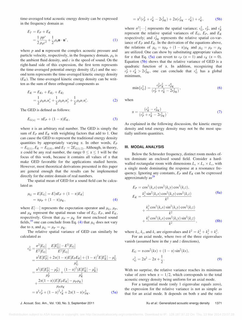
The spatial correlation coefficient for the GED at two field
points can then be calculated as
qEG¼ 1
�2G
a2�2PqEP
þ að1� aÞ�P�KqEP;EKþ ð1� aÞ2�2
KqEK
h i;
(25)
where �2P ¼ 1 and �2
K ¼ 1=3, as indicated earlier. Note that
qEG, as qEP
and qEK, is also a function of r, although it is not
shown explicitly in Eq. (25). There is not a concise expression
for qEG, but some examples for different values of a are plotted
in Fig. 3. It is well accepted that the spatial correlation can be
neglected for the potential energy density if the distance
between two field points is greater than half a wavelength
(0:5k).10 In order to achieve a similarly low level of correlation
(roughly q � 0:05), the separation distance needs to be greater
than approximately 0:8k for EK , ET , and EGð1=4Þ. This may not
be favorable for some applications, such as sound power meas-
urements in a reverberant room, because statistically independ-
ent sampling is required. It is, in some sense, a trade off for
achieving better uniformity. However, for other applications,
i.e., active noise control in diffuse fields,32 a slowly decaying
spatial correlation function may be beneficial.
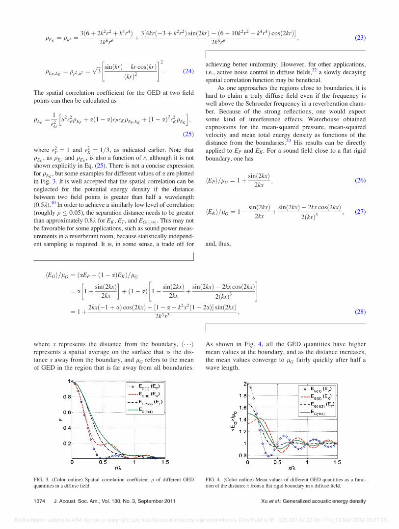
As one approaches the regions close to boundaries, it is
hard to claim a truly diffuse field even if the frequency is
well above the Schroeder frequency in a reverberation cham-
ber. Because of the strong reflections, one would expect
some kind of interference effects. Waterhouse obtained
expressions for the mean-squared pressure, mean-squared
velocity and mean total energy density as functions of the
distance from the boundaries.33 His results can be directly
applied to EP and EK . For a sound field close to a flat rigid
boundary, one has
EPh i=lG ¼ 1þ sinð2kxÞ2kx
; (26)
EKh i=lG ¼ 1� sinð2kxÞ2kx
þ sinð2kxÞ � 2kx cosð2kxÞ2ðkxÞ3
; (27)
and, thus,
EGh i=lG ¼ aEP þ ð1� aÞEKð Þ=lG
¼ a 1þ sinð2kxÞ2kx
� �þ ð1� aÞ 1� sinð2kxÞ
2kxþ sinð2kxÞ � 2kx cosð2kxÞ
2ðkxÞ3
" #
¼ 1þ 2kxð�1þ aÞ cosð2kxÞ þ 1� a� k2x2ð1� 2aÞ½ � sinð2kxÞ2k3x3
; (28)
where x represents the distance from the boundary, � � �h irepresents a spatial average on the surface that is the dis-
tance x away from the boundary, and lG refers to the mean
of GED in the region that is far away from all boundaries.
As shown in Fig. 4, all the GED quantities have higher
mean values at the boundary, and as the distance increases,
the mean values converge to lG fairly quickly after half a
wave length.
FIG. 3. (Color online) Spatial correlation coefficient q of different GED
quantities in a diffuse field.
FIG. 4. (Color online) Mean values of different GED quantities as a func-
tion of the distance x from a flat rigid boundary in a diffuse field.
1374 J. Acoust. Soc. Am., Vol. 130, No. 3, September 2011 Xu et al.: Generalized acoustic energy density
Redistribution subject to ASA license or copyright; see http://acousticalsociety.org/content/terms. Download to IP: 128.187.97.22 On: Thu, 13 Mar 2014 23:07:28

Jacobsen rederived similar results from the stochastic
perspective, and found that both the potential energy density
and all components of kinetic energy density near a bound-
ary (either perpendicular or parallel to the boundary) are in-
dependently distributed with the exponential distribution.10
Therefore, the relative variance of GED near a boundary can
be shown to be
�2EGðxÞ ¼
a2r2EPðxÞ þ ð1� aÞ2r2
EKðxÞ
EGð Þ2; (29)
where
r2EPðxÞ¼ EPð Þ2;
r2EKðxÞ¼ EK?ð Þ2þ2 EKk
� �2
(30)
¼ 1
3þ�2kxcosð2kxÞþ sinð2kxÞ
8k3x3
� �2
þ 1
3� 4kxcosð2kxÞ� 2sinð2kxÞþ 4k2x2 sinð2kxÞ
8k3x3
� �2
;
(31)
where EK? represents the component of EK perpendicular to
the boundary, and EKk represents the component parallel to
the boundary.10 Immediately adjacent to the boundary
(x! 0), Eq. (29) can be simplified to the form
�2EGð0Þ ¼ 2� 4aþ 11a2
ð2þ aÞ2; (32)
which has a minimum value of 1=3 at a ¼ 1=4. Figure 5
plots Eqs. (29) and (32). It is apparent that EGð1=4Þ is more
uniform than EP, EK , and ET everywhere, both near the
boundary and in the region away from the boundary where a
diffuse sound field can be claimed.
V. ENSEMBLE VARIANCE
In a recent publication, Jacobsen obtained the ensemble
variance for the potential, kinetic, and total energy densities
by introducing an independent normally distributed random
variable W to the diffuse field models discussed previ-
ously.15 The variable W has zero mean and a variance of
2=Ms, and is meant to represent the relative variance of the
point source sound power emission associated with the sta-
tistical modal overlap Ms.15 Following his approach, the rel-
ative ensemble variance of GED can be expressed as
�2EG¼
E ½aEP þ ð1� aÞðEKx þ EKy þ EKzÞ�2ð1þWÞ2� �E2 ½aEP þ ð1� aÞðEKx þ EKy þ EKzÞ�ð1þWÞ � � 1
¼3ð1� aÞ2 E E2
Kx
�þ 2E2 EKx½ �
� �þ a2E E2
P
�þ 6að1� aÞE EP½ �E EKx½ �
l2G
1þ E W2 �� �
� 1
¼ 4
3ð1� aÞ2 þ 2a2 þ 2að1� aÞ
� �1þ 2
Ms
� � 1
¼ 8þMs � 2ð2þMsÞaþ 4ð2þMsÞa2
3Ms: (33)
It is interesting to note that the optimal a value is again
1=4, and the minimum variance is 1=4þ 5=2Ms, com-
pared to 1þ 4=Ms for EP and 1=3þ 8=3Ms for both EK
and ET .
The modal overlap can be calculated according to
Ms ¼12p lnð10ÞVf 2
T60c3; (34)
FIG. 5. (Color online) Relative spatial variance of GED close to a flat rigid
boundary bounding a diffuse field. Plot (a) compares the relative variance
for different GED quantities as a function of the distance x from the bound-
ary. Plot (b) shows the relative variance of GED as a function of a at the
boundary (x! 0).
J. Acoust. Soc. Am., Vol. 130, No. 3, September 2011 Xu et al.: Generalized acoustic energy density 1375
Redistribution subject to ASA license or copyright; see http://acousticalsociety.org/content/terms. Download to IP: 128.187.97.22 On: Thu, 13 Mar 2014 23:07:28

where V is the volume of the room and T60 is the reverbera-
tion time.14 Figure 6 plots Eq. (33) for a room with volume
136:6 m3 and a T60 of 6:2 s that is constant over frequency.
VI. NUMERICAL VERIFICATION
A hybrid modal expansion model34 was applied to com-
pute the internal sound field (both complex pressure and
complex particle velocity) of a rectangular room with dimen-
sions 5:4 m� 6:3 m� 4:0 m. The room is very lightly
damped with a uniform wall impedance z ¼ ð50þ 100iÞq0cand a Schroeder frequency of 347:6 Hz. Both the complex
pressure and complex particle velocity fields are computed
over the bandwidth of 50–1000 Hz with 1 Hz increment.
Because of the fast convergence rate of the hybrid model,
only about 3� 104 modes were required for even the highest
frequency. The source location was randomly selected for
each frequency.
The relative variance of EG with different a values is
estimated by calculating the relative variance for EG at 100
randomly selected receiver locations inside the room. The
receiver locations are chosen to be at least a half wavelength
away from the source as well as the boundary. The relative
variance for 100 samples is then averaged over ten frequency
bins to simulate the ensemble variance.15,18 As shown in
Fig. 7, the simulation results match the theoretical predic-
tions reasonably well (compare Fig. 6). The variation of the
curves in Fig. 7 is due to the modal effects. Strictly speaking,
in order to simulate the ensemble variance, a large (ideally
infinite) number of rooms that vary in dimensions need to be
considered. Averaging over a frequency band can only com-
pensate for the lack of room variation to some degree.
The spatial correlation coefficient was estimated at 800
Hz using 11 000 pairs of field points randomly sampled with
the constraint that the separation distance between any two
points of a pair is less than one and a half wavelengths. In
addition, the sampling process was carefully designed so
there were about 500 pairs falling into each of 22 intervals
that equally divided one and a half wavelengths. The spatial
correlation coefficient was calculated for each interval based
on the samples. The results are shown in Fig. 8. Although
the frequency (800 Hz) is above the Schroeder frequency
(347:6 Hz), the sound field still does not correspond to an
ideal diffuse field; therefore some variations are apparent in
the numerical results. Nonetheless, in general, the simulation
results are in fairly good agreement with the theoretical pre-
dictions shown in Fig. 3.
VII. APPLICATIONS
One of the key elements of many applications in a rever-
beration chamber is the estimation of the statistical mean of
the sound field based on a finite number of sampling loca-
tions. Two somewhat contradictory requirements, however,
have to be met in order to achieve a good estimation: (1) the
sound field being sampled at a sufficient number of locations
to achieve the desired level of uncertainty and (2) the choice
of the locations being random, independent, and limited to
the diffuse field region to eliminate bias. Historically,
squared pressure has been the predominant measurement
focus in reverberation chambers, because it is relatively easy
to measure. However, because of its larger spatial variance,
its use does not help resolve the conflict stated above and
may end up either requiring more effort to select measure-
ment locations or a sacrifice in accuracy. Based on the capa-
bility of GED to achieve smaller spatial variance, the
following preliminary studies have demonstrated its utility
in acoustical measurements and active noise control.
A. Reverberation time estimation
In the paper by Nutter et al.,27 the procedure of the
reverberation time (T60) estimation based on the totalFIG. 7. (Color online) Numerical simulation results for the ensemble var-
iance of different GED quantites for a lightly damped room.
FIG. 8. (Color online) Numerical simulation results for the spatial correla-
tion coefficient of GED in a diffuse field.
FIG. 6. (Color online) Ensemble variance of different GED quantities for a
reverberation chamber with V ¼ 136:6 m2 and uniform T60 ¼ 6:2 s.
1376 J. Acoust. Soc. Am., Vol. 130, No. 3, September 2011 Xu et al.: Generalized acoustic energy density
Redistribution subject to ASA license or copyright; see http://acousticalsociety.org/content/terms. Download to IP: 128.187.97.22 On: Thu, 13 Mar 2014 23:07:28

acoustic energy density is investigated in detail. It was
shown for varying numbers of sensor locations that a small
number of energy density measurements can achieve the
same accuracy as larger numbers of pressure measurements.
The impulse responses of multiple source-receiver locations
were obtained for both acoustic pressure and particle veloc-
ity, from which an impulse response associated with the total
energy density, hET, was computed as
hETðtÞ ¼ 1
2q0c2h2
pðtÞ þq0
2h2
uðtÞ; (35)
where hp and hu represent the impulse responses of acoustic
pressure and particle velocity, respectively. The filtered
impulse for each frequency band of interest was then back-
ward integrated to reduce the estimation variance.35 After
averaging the backward integrated curves for the source-re-
ceiver combinations, T60 values could be estimated from the
slopes of the averaged curves. To utilize GED, the procedure
is very much the same, except that the impulse response
associated with GED is calculated by changing the coeffi-
cients in Eq. (35) from 1=2 to a and 1� a for the first and
second terms, respectively.
Reverberation times were thus obtained for a reverbera-
tion chamber based on GED with different values of a. The
reverberation chamber dimensions were 4:96 m� 5:89 m
� 6:98 m. Its volume was 204 m3 and it incorporated sta-
tionary diffusers. The Schroeder frequency for the chamber
was 410 Hz without the presence of low-frequency absorbers.
A dodecahedron loudspeaker was placed sequentially at two
locations within the chamber and driven by white noise. The
acoustic pressure and particle velocity fields were sampled
with a GRAS six-microphone probe at six chamber locations
for each source location. The probe consisted of three pairs of
phase-matched 1=2-inch microphones mounted perpendicular
to each other with spacers, so three orthogonal particle veloc-
ity components could be estimated based on the pressure dif-
ferences. The spacing between microphones in each pair was
5 cm, which is optimal for the frequencies below 1000 Hz.
The acoustic pressure was estimated by averaging the pres-
sure signals from all six microphones in the probe.
The impulse responses were computed by taking the
inverse Fourier transform of the frequency responses between
the acoustic pressure or particle velocity signals and the white
noise signal input to the source. Technically, these impulse
responses represent responses of both the chamber and the
dodecahedron loudspeaker. However, the impulse response
of the loudspeaker was too short to appreciably influence the
T60 estimations. The impulse responses were filtered with
one-third-octave band filters and backward integrated to esti-
mate the T60 values within the bands. Figure 9(a) compares
the averaged T60 estimation based on GED with different avalues. The various GED quantities result in almost identical
reverberation times in most one-third-octave bands. However,
the variance due to source-receiver locations differs, espe-
cially in the low frequency range. As shown in Fig. 9(b), the
estimations based on EK , ET , and EGð1=4Þ have notably less
variance than EP. Less variance implies a smaller number of
measurements or better accuracy. Although the improvement
over EK and ET is not large, the variance is the smallest for
EGð1=4Þ. Considering that there is essentially no additional
effort added for measuring EG as compared to EK and ET ,
EGð1=4Þ is recommended.
B. Sound power measurement in a reverberationchamber
Sound power measurements based on the use of kinetic
energy density or total energy density were also investigated
by Nutter et al.27 Their procedure is relatively simple and
very similar to that based on the squared pressure method
described in the ISO 3741 standard.36 The spatially averaged
sound level is the key parameter in the sound power estima-
tion. In general, the more spatially uniform the sound field
is, the fewer measurements are required to estimate the aver-
aged sound level. The sound power measurement based on
GED was investigated experimentally with the same equip-
ment and in the same reverberation chamber described in the
previous section. With the source being placed close to a
corner in the reverberation chamber (the source was about
1:5 m away from the floor and walls), the GED field was
sampled with the microphone gradient probe at six well sep-
arated locations (at least 1:5 m apart). The locations were
randomly chosen with the constraint of being at least 1:5 m
from the source and the walls. Figure 10(a) shows the
averaged GED levels, which can be calculated as
LG ¼ 10 logðEG=EGrefÞ, where EGref ¼ ð20lPaÞ2=ð2q0c2Þ.The agreement among different a values is good below the
1 kHz one-third-octave band. Above that frequency, the esti-
mations diverge due to the increased errors caused by the
pressure gradient technique. The large difference at 100 Hz
FIG. 9. (Color online) Reverberation time measurements using GED. (a)
Averaged T60 estimation based on different GED quantities for a reverbera-
tion chamber. (b) Variance of the T60 estimations due to the different
source-receiver locations.
J. Acoust. Soc. Am., Vol. 130, No. 3, September 2011 Xu et al.: Generalized acoustic energy density 1377
Redistribution subject to ASA license or copyright; see http://acousticalsociety.org/content/terms. Download to IP: 128.187.97.22 On: Thu, 13 Mar 2014 23:07:28

is caused by the large variance for the sound level of EP.
This can be seen in Fig. 10(b), which shows the standard
deviation of the sound level for different measurement loca-
tions and different GED a values. Again, less variance for
GED with a < 1 can be observed, especially in the low-fre-
quency range. In general, the sound level of EGð1=4Þ has the
smallest standard deviation, but the improvement is not too
dramatic when compared to EK and ET . However EGð1=4Þ is
again recommended due to its improved uniformity with a
measurement effort similar to those of ET and EK .
For the results presented here, the focus is on comparing
results obtained using GED with various values of a. It should
be noted that earlier work27 in the same reverberation cham-
ber provided an extensive comparison of results obtained
using pressure measurements and total acoustic energy den-
sity measurements. That work indicated that for applications
where spatial uniformity is desirable, energy density-based
measurements are generally preferable to pressure measure-
ments. The results presented here provide guidance as to what
value of a can be expected to yield the best results for GED-
based measurements.
C. Global active noise cancellation (ANC) in thelow-frequency range of an enclosure
In a lightly damped enclosure, the total acoustic potential
energy can be reduced at resonance frequencies below the
Schroeder frequency by actively minimizing the squared
acoustic pressure at error sensor locations using one or more
secondary sources.37–39 However, for given primary and sec-
ondary source locations, the global attenuation may vary over
a large range for different error sensor placements. At off res-
onance frequencies, negative attenuation can often be
observed. There is an upper-bound limit for the attenuation
that can be achieved by minimizing the global acoustic poten-
tial energy. However, in principle, this requires an infinite
number of error sensors placed in the enclosure. If, instead of
squared pressure, the total acoustic energy density is mini-
mized at discrete locations, the undesirable effects of the
error sensor positions can be reduced.19,26 With the same
number of error sensors, the global attenuation of the total-
energy-density-based ANC is closer to the upper bound limit
than the squared-pressure-based ANC.
In this section, the active noise cancellation based on
GED in a lightly damped enclosure is simulated numerically.
The dimensions of the enclosure are 2:7 m� 3:0 m� 3:1 m
and a few of the normal modes are listed in Table II. One of
the corners of the enclosure sits at the origin with the three
adjoining edges lying along the positive directions of the x, y,
and z axes. One primary source is located close to a corner at
ð0:27 m; 0:3 m; 0:31 mÞ, and one secondary source is located
at ð2:2 m; 2:0 m; 0:94 mÞ. One error sensor is randomly
placed in the enclosure with the only constraint being that it
is at least one wavelength away from both sources. One
TABLE II. Room modes of a lightly damped enclosure (dimensions:
2:7 m� 3 m� 3:1 m).
Mode (0,0,1) (1,2,0) (0,0,2) (2,0,1) (1,2,1) (1,1,2)
Modal frequency (Hz) 54.59 126.10 126.18 126.70 138.45 138.53
FIG. 10. (Color online) Sound level data for sound power measurements
using GED. (a) Spatially averaged sound levels for different GED quantities
in a reverberation chamber where the source under test is placed in a corner
and 1:5 m away from the floor and walls. (b) Standard deviation of sound
levels for the different source-receiver locations.
FIG. 11. (Color online) Average global attenuation using GED-based active
noise cancellation in an enclosure with random error sensor locations. (a)
Average attenuation based on EGð1Þ (EP), EGð0Þ (EK) and EGð1=2Þ (ET). (b)
Average attenuation based on EGð1=2Þ, EGð1=4Þ, EGð1=10Þ and the total potential
energy upper-bound limit. The attenuation based on total potential energy is
considered optimal (Ref. 37).
1378 J. Acoust. Soc. Am., Vol. 130, No. 3, September 2011 Xu et al.: Generalized acoustic energy density
Redistribution subject to ASA license or copyright; see http://acousticalsociety.org/content/terms. Download to IP: 128.187.97.22 On: Thu, 13 Mar 2014 23:07:28

hundred tests were performed, with the secondary source
strength being adjusted each time to minimize GED at the
randomly chosen error sensor location. The bandwidth of 40
to 180 Hz was studied, with 1 Hz increments. The average
attenuation over the tests of the total potential acoustic energy
in the enclosure was compared for the various control
schemes. As shown in Fig. 11(a), the ET-based ANC is nota-
bly better than the EP-based ANC and slightly better than the
EK based ANC. The EP (or squared pressure) based ANC can
result in large boosts (negative attenuation) for off resonance
frequencies, while the EK and ET-based ANC result in much
smaller boosts. Figure 11(b) compares GED-based ANC for
the a values of 1=10, 1=4, and 1=2(ET), along with the upper
bound limit. These three ANC results are very similar. The
EGð1=4Þ-based ANC tends to achieve a slightly better attenua-
tion than the other two. The difference, however, is small
except for the frequencies around 154 Hz. It can also be
observed that the EGð1=4Þ-based ANC generally has less
attenuation variance than the other schemes (Fig. 12).
VIII. CONCLUSIONS
Generalized acoustic energy density (GED) has been
introduced in this paper. When averaged over the volume of
an enclosure, it has the same mean value as the acoustic total
energy density. It can revert to the traditional energy density
quantities, such as acoustic potential energy density, acoustic
kinetic energy density, and acoustic total energy density. By
varying its weighting factors for the combination of acoustic
potential energy density and acoustic kinetic energy density,
an additional degree of freedom is added to the summed
energy density quantity so that it can be optimized for differ-
ent applications. Properties of GED with different values of ahave been studied for individual room modes, diffuse sound
fields, and sound fields below the Schroeder frequency.
The uniformity of a measured sound field often plays an
important role in many applications. This work has shown
that optimal weighting factors based on a single parameter acan minimize the spatial variance of the GED. For a single
room mode, the optimal value of a may vary from 1=10 to
1=2, depending on the specific mode shape. For a diffuse
field, the optimal value is 1=4 for both single frequency and
narrow-band frequency excitations, even for the region close
to a rigid reflecting surface. For a diffuse field excited by a
single tone source, EGð1=4Þ follows the distribution of
Cð4; lG=4Þ and has a relative spatial variance of 1=4, com-
pared to 1=3 for EK and ET . Below the Schroeder frequency
of a room, a smaller ensemble variance can also be reached
when a ¼ 1=4.
Benefits of total-energy-density-based techniques have
been shown in the past. Experimental studies of GED-based
reverberation time and sound power measurements in a
reverberation chamber confirm the improved uniformity of
EGð1=4Þ, especially in the low-frequency region. They indi-
cate that more reliable results may be obtained using EGð1=4Þfor those measurements. Global active noise control in a
lightly damped enclosure has also been studied through com-
puter simulation. The results demonstrated that when
a � 1=2, the average global attenuation is not particularly
sensitive to the specific value of a, but EGð1=4Þ introduces
less variance for the attenuation than other quantities.
In general, EGð1=4Þ based techniques do result in improve-
ments compared to ET and EP based techniques. The degree
of the improvements were not large compared to the ET-
based techniques. However, since EGð1=4Þ requires no addi-
tional effort to implement in most applications, and since it is
very simple to modify existing ET-based techniques, the
EGð1=4Þ-based techniques may be considered to be superior.
1W. C. Sabine, Collected Papers on Acoustics (Dover Publications, New
York, 1964), p. 279.2I. Wolff and F. Massa, “Direct meaurement of sound energy density and
sound energy flux in a complex sound field,” J. Acoust. Soc. Am. 3, 317–
318 (1932).3I. Wolff and F. Massa, “Use of pressure gradient microphones for acousti-
cal measurements,” J. Acoust. Soc. Am. 4, 217–234 (1933).4L. W. Sepmeyer and B. E. Walker, “Progress report on measurement of
acoustic energy density in enclosed spaces,” J. Acoust. Soc. Am. 55, S12
(1974).5R. V. Waterhouse, “Statistical properties of reverberant sound fields,”
J. Acoust. Soc. Am. 43, 1436–1444 (1968).6R. H. Lyon, “Statistical analysis of power injection and response in struc-
tures and rooms,” J. Acoust. Soc. Am. 45, 545–565 (1969).7R. K. Cook and P. A. Schade, “New method for measurement of the total
energy density of sound waves,” Proc. Inter-Noise 74, Washington, DC,
1974, pp. 101–106.8R. V. Waterhouse and R. K. Cook, “Diffuse sound fields: Eigenmode and
free-wave models,” J. Acoust. Soc. Am. 59, 576–581 (1976).9R. V. Waterhouse and D. W. v. W. Palthe, “Space variance for rectangular
modes,” J. Acoust. Soc. Am. 62, 211–213 (1977).10F. Jacobsen, “The diffuse sound field: statistical considerations concerning
the reverberant field in the steady state,” Technical Report, Technical Uni-
versity of Denmark, 1979.
FIG. 12. (Color online) Variance of the attenuation. (a) Variance of the
attenuation for EGð1Þ (EP), EGð0Þ (EK), and EGð1=2Þ (ET). (b) Variance of the
attenuation for EGð1=2Þ, EGð1=4Þ, and EGð1=10Þ.
J. Acoust. Soc. Am., Vol. 130, No. 3, September 2011 Xu et al.: Generalized acoustic energy density 1379
Redistribution subject to ASA license or copyright; see http://acousticalsociety.org/content/terms. Download to IP: 128.187.97.22 On: Thu, 13 Mar 2014 23:07:28

11J. A. Moryl and E. L. Hixson, “A total acoustic energy density sensor with
applications to energy density measurement in a reverberation room,”
Proc. Inter-Noise 87, Beijing, China, Vol. II, pp. 1195–1198.12J. A. Moryl, “A study of acoustic energy density in a reverberation room,”
Ph.D. thesis, The University of Texas at Austin (1987).13R. L. Weaver and J. Burkhardt, “Weak Anderson localization and
enhanced backscatter in reverberation rooms and quantum dots,” J.
Acoust. Soc. Am. 96, 3186–3190 (1994).14F. Jacobsen and A. R. Molares, “Sound power emitted by a pure-tone source
in a reverberation room,” J. Acoust. Soc. Am. 126, 676–684 (2009).15F. Jacobsen and A. R. Molares, “The ensemble variance of pure-tone
measurements in reverberation rooms,” J. Acoust. Soc. Am. 127, 233–237
(2010).16J. L. Davy, “The relative variance of the transmission function of a rever-
beration room,” J. Sound Vib. 77, 455–479 (1981).17R. L. Weaver, “On the ensemble variance of reverberation room transmis-
sion functions, the effect of spectral rigidity,” J. Sound Vib. 130, 487–491
(1989).18F. Jacobsen and A. R. Molares, “Statistical properties of kinetic and total
energy densities in reverberant spaces,” J. Acoust. Soc. Am. 127, 2332–
2337 (2010).19J. W. Parkins, S. D. Sommerfeldt, and J. Tichy, “Error analysis of a practi-
cal energy density sensor,” J. Acoust. Soc. Am. 108, 211–222 (2000).20B. S. Cazzolato and C. H. Hansen, “Errors arising from three-dimensional
energy density sensing in one-dimensional sound fields,” J. Sound Vib.
236, 375–400 (2000).21J. Ghan, B. Cazzolato, and S. Snyder, “Statistical errors in the estimation
of time-averaged acoustic energy density using the two-microphone
method,” J. Acoust. Soc. Am. 115, 1179–1184 (2004).22J.-C. Pascal and J.-F. Li, “A systematic method to obtain 3d finite-differ-
ence formulations for acoustic intensity and other energy quantities,”
J. Sound Vib. 310, 1093–1111 (2008).23H.-E. de Bree, P. Leussink, T. Korthorst, H. Jansen, T. S. J. Lammerink,
and M. Elwenspoek, “The u-flown: A novel device for measuring acoustic
flows,” Sens. Actuators A, 54, 552–557 (1996).24T. G. H. Basten and H.-E. de Bree, “Full bandwidth calibration procedure
for acoustic probes containing a pressure and particle velocity sensor,”
J. Acoust. Soc. Am. 127, 264–270 (2010).
25J. W. Parkins, “Active minimization of energy density in a three-dimen-
sional enclosure,” Ph.D. thesis, The Pennsylvania State University
(1998).26J. W. Parkins, S. D. Sommerfeldt, and J. Tichy, “Narrowband and broad-
band active control in an enclosure using the acoustic energy density,”
J. Acoust. Soc. Am. 108, 192–203 (2000).27D. B. Nutter, T. W. Leishman, S. D. Sommerfeldt, and J. D. Blotter,
“Measurement of sound power and absorption in reverberation chambers
using energy density,” J. Acoust. Soc. Am. 121, 2700–2710 (2007).28P. M. Morse and R. H. Bolt, “Sound waves in rooms,” Rev. Mod. Phys.
16, 69–150 (1944).29D. Lubman, “Fluctuations of sound with position in a reverberant room,”
J. Acoust. Soc. Am. 44, 1491–1502 (1968).30R. K. Cook, R. V. Waterhouse, R. D. Berendt, S. Edelman, and J. M. C.
Thompson, “Measurement of correlation coefficients in reverberant sound
fields,” J. Acoust. Soc. Am. 27, 1072–1077 (1955).31D. Lubman, “Spatial averaging in a diffuse sound field,” J. Acoust. Soc.
Am. 46, 532–534 (1969).32S. J. Elliott, P. Joseph, A. J. Bullmore, and P. A. Nelson, “Active cancellation at
a point in a pure tone diffuse sound field,” J. Sound Vib. 120, 183–189 (1988).33R. V. Waterhouse, “Interference patterns in reverberant sound fields,”
J. Acoust. Soc. Am. 27, 247–258 (1955).34B. Xu and S. D. Sommerfeldt, “A hybrid modal analysis for enclosed
sound fields,” J. Acoust. Soc. Am. 128, 2857–2867 (2010).35M. R. Schroeder, “New method of measuring reverberation time,”
J. Acoust. Soc. Am. 37, 409–412 (1965).36ISO 3741:1999(E), “Acoustics—Determination of sound power levels of
noise sources using sound pressure—Precision methods for reverberation
rooms” (International Organization for Standardization, Geneva, 1999).37P. A. Nelson, A. R. D. Curtis, S. J. Elliott, and A. J. Bullmore, “The active
minimization of harmonic enclosed sound fields, part I: Theory,” J. Sound
Vibr. 117, 1–13 (1987).38A. J. Bullmore, P. A. Nelson, A. R. D. Curtis, and S. J. Elliott, “The active
minimization of harmonic enclosed sound fields, part II: A computer simu-
lation,” J. Sound Vibr. 117, 15–33 (1987).39S. J. Elliott, A. R. D. Curtis, A. J. Bullmore, and P. A. Nelson, “Active
minimization of harmonic enclosed sound fields, part III: Experimental
verification,” J. Sound Vibr. 117, 35–58 (1987).
1380 J. Acoust. Soc. Am., Vol. 130, No. 3, September 2011 Xu et al.: Generalized acoustic energy density
Redistribution subject to ASA license or copyright; see http://acousticalsociety.org/content/terms. Download to IP: 128.187.97.22 On: Thu, 13 Mar 2014 23:07:28
Recommended