
Forecasting commodity currencies: the role of fundamentals with short-lived predictive content
NORGES BANKRESEARCH
14 | 2015
AUTHORS: CLAUDIA FORONI,FRANCESCO RAVAZZOLO ANDPINHO J. RIBEIRO
WORKING PAPER

NORGES BANK
WORKING PAPERXX | 2014
RAPPORTNAVN
2
Working papers fra Norges Bank, fra 1992/1 til 2009/2 kan bestilles over e-post: [email protected]
Fra 1999 og senere er publikasjonene tilgjengelige på www.norges-bank.no Working papers inneholder forskningsarbeider og utredninger som vanligvis ikke har fått sin endelige form. Hensikten er blant annet at forfatteren kan motta kommentarer fra kolleger og andre interesserte. Synspunkter og konklusjoner i arbeidene står for forfatternes regning.
Working papers from Norges Bank, from 1992/1 to 2009/2 can be ordered by e-mail:[email protected]
Working papers from 1999 onwards are available on www.norges-bank.no
Norges Bank’s working papers present research projects and reports (not usually in their final form) and are intended inter alia to enable the author to benefit from the comments of colleagues and other interested parties. Views and conclusions expressed in working papers are the responsibility of the authors alone.
ISSN 1502-8143 (online) ISBN 978-82-7553-879-4 (online)

Forecasting Commodity Currencies:
The Role of Fundamentals with Short-Lived
Predictive Content∗
Claudia Foroni†, Francesco Ravazzolo‡, Pinho J. Ribeiro§
October 30, 2015
Abstract
Recent evidence highlights that commodity price changes exhibit a short-lived, yet ro-
bust contemporaneous effect on commodity currencies, which is mainly detectable in daily-
frequency data. We use MIDAS models in a Bayesian setting to include mixed-frequency
dynamics while accounting for time-variation in predictive ability. Using the random walk
Metropolis-Hastings technique as a new tool to estimate our class of MIDAS regressions, we
find that for most of the commodity currencies in our sample exploiting this short-lived re-
lationship yields to statistically more precise out-of-sample exchange rate point and density
forecasts relative to the no-change benchmark. Further, the usual low-frequency predictors,
such as money supplies and interest rates differentials, typically receive little support from
the data at monthly forecasting horizons. In contrast, models featuring daily commodity
prices are highly likely.
Keywords: Exchange rate point and density forecasting; Commodity prices; MIDAS model;
Bayesian model averaging; Metropolis-Hastings algorithm
JEL Classification: C53, C55, F37.
∗This working paper should not be reported as representing the views of Norges Bank. The views expressedare those of the authors and do not necessarily reflect those of Norges Bank. We benefited from constructivecomments by Raffaella Giacomini, Barbara Rossi, and seminar participants at Norges Bank. This research wasconducted while Ribeiro was a Ph.D. Intern at Norges Bank. Correspondence to: Pinho Ribeiro, University ofGlasgow, Adam Smith Building, Glasgow G12 8RT - United Kingdom. E-mail: [email protected]†Norges Bank.‡Norges Bank and Centre for Applied Macro and Petroleum Economics at BI Norwegian Business School.§University of Glasgow, Adam Smith Business School.
1 Introduction
Exchange rate fluctuations constitute a major source of risk to several economic agents. Not
surprisingly, academics, market practitioners and policymakers have long been concerned about
the determinants of exchange rate movements. In their seminal paper, Meese and Rogoff (1983)
examine whether exchange rate fluctuations can be predicted using macroeconomic variables.
They show that forecasts based on standard models that relate exchange rates dynamics to
macroeconomic variables do not outperform forecasts based on a driftless random walk. Their
results triggered a large literature examining the weak predictive power of macroeconomic vari-
ables on exchange rates, and three decades later, Rossi (2013) notes that Meese and Rogoff’s
(1983) findings have not yet been overturned. As she points out, the main issue is that the pre-
dictive ability of macroeconomic fundamentals is ephemeral.1 In other words, although some
fundamentals exhibit predictive content at short horizons and others at long horizons, none of
them have systematic forecasting power.
In a recent paper, however, Ferraro et al. (2015) suggest that the frequency of the data used
in the predictive regressions for exchange rates may be important in pinning down forecasting
ability. They argue that the most probable reason for the failure to uncover predictive power
in fundamentals such as commodity prices is the emphasis of the literature on data sampled at
low frequency. At this frequency, the predictive content of this sort of fundamental is transitory.
In fact, using monthly/quarterly data on oil price changes to predict fluctuations in exchange
rates at similar frequencies, Ferraro et al. (2015) hardly detect predictive content (see also
Chen et al., 2010 for congruent results). When instead they regress the contemporaneous daily
change in the exchange rate on the current daily fluctuation on oil prices, they find a significant
and consistent relationship. The relationship is short-lived, in the sense that it can mainly
be detected using high frequency data and it washes away quickly. Indeed, in a strict out-of-
sample exercise, where lagged rather than contemporaneous daily price changes are used to
predict future exchange rate movements, predictability is found to be time-varying and subject
to large instabilities.
In this paper we employ a systematic approach to exploit the short-lived effect of commodity
prices on exchange rates, in a pseudo out-of-sample context. In contrast with the existing
1A very limited list of other papers highlighting this conclusion includes Berge (2013), Fratzscher at al.(2015), Giacomini and Rossi (2010), Ferraro et al. (2015), Rogoff and Stavrakeva (2008) and Sarno and Valente(2009).
1
exchange rate studies, we allow the effect of daily fluctuations in commodity prices to carry on
to the end-of-month change in the exchange rate. Using the so-called MIxed DAta Sampling
(MIDAS) framework, each daily observation on price fluctuations can have a different weight or
impact on the end-of-month observation on the exchange rate change. The MIDAS regression
is a simple, parsimonious, and flexible modeling approach that allows the variables entering
a time series regression to be sampled at different frequencies (Ghysels, 2007). For instance,
fluctuations at the end of the month can have more predictive power than fluctuations further
back. With our approach we can attribute more importance to these observations that are
closer in time, while the literature typically would aggregate them to the lowest frequency with
equal weights.
Further, the empirical literature also suggests that the predictive content of either commod-
ity prices or the standard macroeconomic fundamentals is time-varying. Ferraro et al. (2015),
for example, find that lagged daily fluctuations in oil prices were better predictors of daily
changes in the Canadian/U.S. dollar exchange rate around 2006-2007, while at the monthly and
quarterly frequencies predictive ability is never found.2 Hence, in our approach, we let each of
the high-frequency commodity prices we consider be potentially relevant at each point in time.
More specifically, our MIDAS predictive models allow for changing sets of high and/or low fre-
quency regressors at each period in time. In this setting, we make two additional contributions.
First, we use a likelihood-based approach to shed light on whether regressors sampled at high
frequency are more informative about monthly changes in exchange rates than predictors sam-
pled at low/same frequency. Second, we equally employ the likelihood information to account
for potential time-variation in the predictive content of our predictors (i.e., commodity prices
and standard macroeconomic fundamentals). Therefore, we forecast with the predictors with
the highest support from the data at each period in time. Alternatively, we compute the fore-
cast as a weighted average of each model’s forecast. In this methodical manner, we analyze if
accounting for the time-changing predictive ability improves forecast accuracy. More generally,
in our framework, we check whether the predictive content of fundamentals sampled at high
and low frequency should be regarded as complementary, rather than substitute of commodity
prices.
All our models are estimated with Bayesian methods, and we introduce the random walk
2See also an explanation for the time-variation in predictive content based on a scapegoat theory of exchangerates of Bacchetta and van Wincoop (2004, 2013) or the empirical evidence in Fratzscher et al. (2015).
2
chain Metropolis-Hastings algorithm as a tool for estimating MIDAS regressions. Bayesian
methods are progressively being applied in MIDAS papers, owing to their advantage in terms
of providing a systematic framework to incorporate model and parameter uncertainty by focus-
ing on the full predictive density (see Pettenuzzo et al., 2015, for a recent application). These
methods also allow us to systematically achieve our goals of (i) examining the degree of infor-
mativeness of predictors sampled at different frequencies and (ii) accounting for time-variation
in forecasting performance.
We focus on commodity prices/currency pairs of three major commodity exporting coun-
tries: (a) Australia with emphasis on gold and copper prices; (b) Canada, concentrating on oil
and copper prices, and (c) Norway with oil and gas prices. In addition, following the indication
in Chen et al. (2010) that commodity price movements may induce exchange rates fluctuations
for large commodity importers, we examine the case of Japan (focusing on oil prices and a com-
modity price index), as an example of this category of countries. Overall, while our left-hand
side variable is always sampled at monthly frequency, on the right-hand-side our regressions
allow for commodity prices sampled at daily or monthly frequency, or standard macroeconomic
predictors sampled at monthly frequency (e.g., interest rate differentials, money supply differ-
entials, and price differentials).
Using monthly and the corresponding daily data from September 1986 to March 2014 we
recursively forecast the 1–month ahead change in the exchange rate. Our forecasts are com-
pared to those of the driftless Random Walk, which according to Rossi (2013), is the toughest
benchmark in the exchange rate literature. To assess the forecasting performance of our meth-
ods we employ the root mean squared forecast error (RMSFE) for point forecasts and log-score
differentials for density forecasts. We examine the statistical significance of our forecasts using
the Clark and West (2006, 2007) test-statistic.
What we find is that exploiting the properties of daily commodity prices in a MIDAS set-
ting leads to forecast improvements. In terms of point forecasts for example, MIDAS regressions
with daily copper prices improve upon the RW benchmark for the Australian dollar and the
Canadian dollar. In contrast, and consistent with the existing evidence, standard regressions
with commodity prices sampled at low frequency hardly improve upon our benchmark. Regard-
ing density forecasts, our results suggest that once we account for the full forecast distribution,
the RW never forecasts better than the commodity or fundamentals-based regressions. As well,
when we account for time-variation in forecasting ability by combining the forecasts from our
3
MIDAS models and from regressions based on standard macroeconomic fundamentals we also
improve upon the RW. Inspection of the data-driven weights underlying our forecast combi-
nations approaches reveals that daily commodity prices are relatively more informative about
monthly changes in exchange rates than monthly commodity prices or the typical macroeco-
nomic variables.
The paper proceeds as follows. In Section 2 we use a small simulation example to illustrate
why a MIDAS setup might be appropriate to pin down the forecasting ability of daily commodity
prices. In Section 3 we detail our methodology, including our new contribution in terms of
estimation of MIDAS regression using the random walk Metropolis-Hastings algorithm. Section
4 describes the essential features of our empirical exercise. In Section 5 we report our main
forecasting results. Section 6 examines the empirical attributes underlying our Bayesian forecast
combination methods. Robustness checks are in Section 7, while Section 8 concludes.
2 A Small Simulation Example
To visualize the importance of considering our approach, Figure 1 shows a simulation exercise
based on the moments (mean and standard deviation) taken from the data we consider in
our empirical section. The econometric procedure underlying the simulation is detailed in the
methodological section.
In Panel A we assume a Data Generating Process (DGP) in which monthly fluctuations
in the exchange rate, ∆st, are driven by a daily-frequency variable, denoted xtd, where each
observation is allowed to have a different effect on ∆st. The simulated DGP is:3
∆st= −0.001 + 0.50× [f(θ1, θ2)(xtd21+xtd20+...+ xd1)]+εt (1)
where εt is an i.i.d. error term with var(εt) = 0.11. The subscript d() attached to xt indicates the
occurrence of the daily observation in a month. Essentially, we consider 22 working days within a
month. Further, we assume that the previous 21 daily observations affect the value of ∆st. The
function, f(θ1, θ2), is a polynomial that allows us to smooth the past daily observations on the
basis of the two parameters. We set these parameters to θ1= 0.3 and θ2 = −0.1, implying that
for this DGP, observations close to the end of the month have higher impact on ∆st than those at
3The DGP is a MIDAS model based on the exponential Almon lag polynomial with the parameters thatdetermine the weights defined by θ1and θ2. A complete description of this type of model is given in Section 3.
4
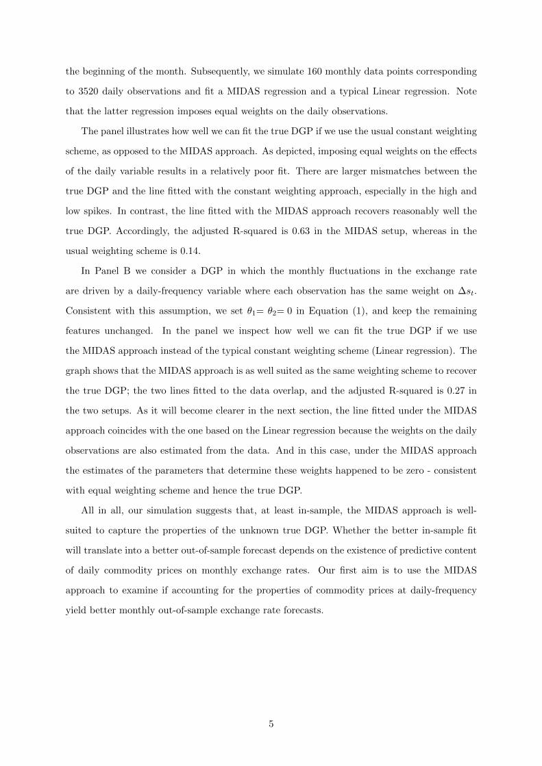
the beginning of the month. Subsequently, we simulate 160 monthly data points corresponding
to 3520 daily observations and fit a MIDAS regression and a typical Linear regression. Note
that the latter regression imposes equal weights on the daily observations.
The panel illustrates how well we can fit the true DGP if we use the usual constant weighting
scheme, as opposed to the MIDAS approach. As depicted, imposing equal weights on the effects
of the daily variable results in a relatively poor fit. There are larger mismatches between the
true DGP and the line fitted with the constant weighting approach, especially in the high and
low spikes. In contrast, the line fitted with the MIDAS approach recovers reasonably well the
true DGP. Accordingly, the adjusted R-squared is 0.63 in the MIDAS setup, whereas in the
usual weighting scheme is 0.14.
In Panel B we consider a DGP in which the monthly fluctuations in the exchange rate
are driven by a daily-frequency variable where each observation has the same weight on ∆st.
Consistent with this assumption, we set θ1= θ2= 0 in Equation (1), and keep the remaining
features unchanged. In the panel we inspect how well we can fit the true DGP if we use
the MIDAS approach instead of the typical constant weighting scheme (Linear regression). The
graph shows that the MIDAS approach is as well suited as the same weighting scheme to recover
the true DGP; the two lines fitted to the data overlap, and the adjusted R-squared is 0.27 in
the two setups. As it will become clearer in the next section, the line fitted under the MIDAS
approach coincides with the one based on the Linear regression because the weights on the daily
observations are also estimated from the data. And in this case, under the MIDAS approach
the estimates of the parameters that determine these weights happened to be zero - consistent
with equal weighting scheme and hence the true DGP.
All in all, our simulation suggests that, at least in-sample, the MIDAS approach is well-
suited to capture the properties of the unknown true DGP. Whether the better in-sample fit
will translate into a better out-of-sample forecast depends on the existence of predictive content
of daily commodity prices on monthly exchange rates. Our first aim is to use the MIDAS
approach to examine if accounting for the properties of commodity prices at daily-frequency
yield better monthly out-of-sample exchange rate forecasts.
5
3 Methodology
3.1 Predictive MIDAS Model
In our empirical analysis, we are firstly interested in forecasting the h-month-ahead change in
the exchange rate, using a predictor sampled daily. The usual procedure would be to aggregate
the data on the daily-frequency variable to match the frequency of the low-sampled one. As
shown in Section 2, this aggregation might result in a poor fit, as well as loss of the properties
of the data, and econometric estimation issues related to inconsistent estimators (see Andreou
et al., 2010). To potentially avoid these issues, a MIDAS regression allows mixing variables
sampled at different frequencies. A simple MIDAS regression for our forecasting problem is:
∆st+h = β0 + β1B1(L1/m; θ1)x
(m)t + εt+h; εt+h ∼ N(0, σ2), (2)
where
β1B1(L1/m; θ1) ≡ B(L1/m; θ) =
K−1∑k=0
B(k; θ)Lk/m, (3)
for t = 1, ..., T − h, and h = 1 (a similar model is used by Pettenuzzo et al., 2015).
In Equation (2), ∆st+h is the period-ahead change in the exchange rate at monthly frequency.
Our daily regressor, denoted x(m)t , is sampled m times between t and t+1, and m = 22 assuming
that there are always 22 observations within a month.4 The key ingredient in the MIDAS model
is the polynomial function, B(L1/m; θ), which allows to smooth K past observations of x(m)t on
the basis of a few number of parameters θ = (θ0, θ1, ..., θp), where p+ 1 << K. In this function,
Lk/m is a lag operator such that L1/mx(m)t = x
(m)t−1/m, i.e., we denote lags of x
(m)t by x
(m)t−j/m.
Once the parameters of this function are obtained, the effect of past values of x(m)t on ∆st+h is
captured by β1.
To gain insights on these concepts, consider for instance that a time t monthly change
in the exchange rate is affected by the previous 21 daily observations of x(m)t . Without using
a smoothing function or restricting the parameters in B(L1/m; θ), we would have to include
K = 21 daily lags in Equation (2) and estimate 21 + 2 parameters. Instead, in a MIDAS
4To create balanced monthly observations we assume the following. First, for months with less than 22observations, we consider that the observation in the last working day of the previous month extends to one daybefore the first working day of the current month. If this does not complete 22 days, we further posit that thelast observation of the current month is valid for one extra day. Second, for months with more than 22 days,typically 23, we average the first two daily observations.
6
regression the smoothing function, B(L1/m; θ), uses fewer parameters (two in our application).
We can extend the model in (2) to include n other regressors, zt = (z1t, ..., znt)′, sampled at
the same frequency as ∆st+h:
∆st+h = β0 + β1B(L1/m; θ1)x(m)t + δ′zt + εt+h, (4)
where δ is a vector of n coefficients associated with zt. The model in (4) nests two specifications
that we consider in our empirical work: (i) a MIDAS model if we exclude the predictors in zt
and (ii) a typical Linear regression, if we exclude the daily (x(m)t ) variables and forecast the
monthly change in the exchange only with commodity prices or macroeconomic fundamentals
sampled at the same frequency as ∆st+h.
To complete the specification of the MIDAS regression we need to define the functional
form of the polynomial B(L1/m; θ). While several alternatives exist, and the adoption of any
particular depends on the application at hand, we employ the exponential Almon lag polynomial
following Ghysels et al. (2007):5
B(k; θ) =e(θ1k+θ2k
2)∑Ki=1 e
θ1i+θ2i2, (5)
with θ = (θ1, θ2). This polynomial is flexible enough to take various shapes for different values
of its parameters, (θ1, θ2), and Ghysels et al. (2005) have found it to work well in practice.
If we consider that only the past 21 trading days affect the value of ∆st+h, then under this
polynomial Equation (2) is a compact representation of:
∆st+h = β0+β1
(e(θ1×1+θ2×1
2)∑Ki=1 e
θ1i+θ2i2xtd21 +
e(θ1×2+θ2×22)∑K
i=1 eθ1i+θ2i2
xtd20 + ...+e(θ1×21+θ2×21
2)∑Ki=1 e
θ1i+θ2i2xtd1
)+εt+h.
(6)
This MIDAS regression is non-linear, requiring non-linear methods for estimation. We focus on
an appropriate algorithm to implement in the next subsection.
5In our empirical exercise we also experimented with the unrestricted MIDAS approach of Foroni et al.(2013). In unreported results we find that forecasts based on this approach were generally less precise than theRW benchmark. A possible explanation for this weak performance might be the loss of precision in parameterestimates, since in this approach and given our daily-frequency predictors, a relatively large number of parametershave to be estimated.
7
3.2 Bayesian Estimation and Forecasting
We use Bayesian methods to estimate the parameters of our regressions. These methods are
increasingly being applied in MIDAS studies (see, e.g., Pettenuzzo et al., 2015 and references
there in). The major advantage of Bayesian techniques over the typical frequentist methods is to
account for model and parameter uncertainty. This is achieved by obtaining the full predictive
density, rather than solely a point forecast underlying the frequentist approach. As we elaborate
next, in a Bayesian setup we can also combine forecasts in a more methodical fashion.
To describe the mechanics of our novel MIDAS estimation techniques with a simple notation,
first express Equation (6) in the following functional form:
S = f(X, γ)+ε, ε ∼ N(0,1
η), and
1
η= σ2; (7)
where we have suppressed, for notational simplicity, the dependence on the forecast horizon h
and time t. Moreover, f(.) indicates that our function of interest depends on the data (X) and
parameters in γ, where X contains our daily predictors (xtd), and γ includes the parameters
β0, β1, θ1, θ2.
Bayesian estimation involves the definition of prior distributions, the likelihood function,
and the posterior distribution. We use independent Normal-Gamma priors. As such, the prior
for γ is independent of the prior for η and is defined as:
γ ∼ N(γ, V ). (8)
For the error precision, η, the prior is:
η ∼ G(s−2, ν). (9)
We set γ = (0, 0, 0, 0)′, V = 0.35I, ν = 1, and s−2 is based on OLS estimate of Equation (2)
assuming that the data is aggregated to the monthly frequency under the constant weighting
scheme. All these choice of priors are sensible but relatively diffuse. For instance, the elements
of the prior mean in γ incorporate the view that the driftless Random Walk model provides
better exchange rate forecasts. At the same time, the prior variance, V , allows the coefficients
estimates to wander in the region [−1.2, 1.2] with 95% prior probability assuming normality.
We further note that only data available up to the beginning of our first forecast are used to
8
estimate any data-based quantity such as s−2.
If we combine these priors with the likelihood we obtain the following conditional posterior
for η (see Appendix A for details):
p(η|S,γ) ∼ G(s−2,ν), (10)
where s2 = [S−f(X,γ)]′[S−f(X,γ)]+νs2ν and ν = ν + T. As shown in Koop (2003, Ch. 5), the
conditional posterior distribution of γ is:
p(γ|S, η) ∝ exp[−η
2
{S − f(X, γ)}′{S − f(X, γ)
}](11)
exp
[(−1
2(γ−γ)′V −1(γ−γ))
].
This latter conditional posterior (p(γ|S, η)) does not suggest any density from which to directly
sample from. We propose the random walk chain Metropolis-Hasting (RW-MH) posterior sim-
ulator to sequentially draw parameters from a suitable candidate generating density, in the
spirit of Koop (2003, Ch. 5). Essentially, candidate draws of γ, denoted by γ∗, are generated
according to a random walk. Following a typical procedure, we choose the multivariate Normal
distribution as the candidate generating density:
q(γ(dr−1), γ) ∼ fN(γ|γ(dr−1),Σ), (12)
where γ(dr−1) denotes the last accepted draw of γ, and Σ is a pre-selected covariance matrix
which guarantees that the acceptance probability is within a reasonable range, typically [0.2, 0.5].
Using data available up to the beginning of our first forecast we set this covariance matrix to
the maximum likelihood variance estimate, Σ = var(γ̂ML). The acceptance probability of the
candidate draw is calculated as:
a(γ(dr−1), γ∗) = min
[p(γ = γ∗|S, η)
p(γ = γ(dr−1)|S, η), 1
]. (13)
with p() at the current and previous draw evaluated using Equation (11).
The RW-MH algorithm simulates draws for p(γ|S, η), but we also require draws from
p(η|S,γ). Since we know the form of this density (see Equation (10)), we can easily com-
bine the RW-MH step with the Gibbs sampler. Such Metropolis-within-Gibbs algorithm allows
9
us to sequentially draw η conditional on γ. Refer to Appendix A for further details and exact
steps.
To forecast with our model we need the predictive density. This is given by:
p(S∗|S, γ) = t(S∗|f(X∗, γ), s2IT , T ), (14)
where s2 = (S−f)′(S−f)/T. Using the Gibbs sampler we can obtain draws from this predictive
density, from which we can compute point and density forecasts. In our empirical exercise, we
generate 31000 draws from which we discard the first 1000 and keep every third draw for
inference. Details about the convergence measures are relegated to Appendix C.6
3.3 Bayesian Model Averaging or Selection and Optimal Predictive Pool
So far we have focused on estimating and forecasting with a model defined according to the
predictors it includes. Since we estimate and obtain predictive densities for several alternative
models at each point in time, we can optimally exploit the predictive content of each predictor.
For example, we compute forecast combinations based on each model’s relative importance over
time. Alternatively, we forecast with the model that yields the highest weight (i.e., probability)
at each point in time or compute the optimal predictive pool of Geweke and Amisano (2011).
The first two approaches assume that the true model is in the model set and the selection
or combination converges asymptotically to it. The optimal predictive pool, on the contrary,
allows for model incompleteness, meaning the true model might not be present in the model set,
see Mitchell and Hall (2007) and Geweke and Amisano (2011). Moreover, apart from allowing
to account for instabilities in the model’s forecasting performance, the weights permit to make
inference about which predictors are more informative about exchange rate fluctuations.
To visualize these weighting and forecasting schemes, let Mi identify a specific model from
the set of MN models, such that the predictive density in (14) is now also model-specific,
p(S∗|S, γ,Mi). Bayesian Model Selection (BMS) uses weights derived from the realized likelihood
of the model’s prediction to select a single model. Bayesian Model Averaging (BMA) employs
the weights to average results over all models.
The starting point is to assign prior probabilities to each model, and subsequently obtaining
6We checked the convergence and adequacy of the number of draws using standard procedures, such asGeweke’s (1992) numerical standard errors (NSE) and acceptance rates in the RW-MH algorithm. Overallresults indicate an acceptable degree of efficiency of the algorithm.
10
posterior probabilities (weights) based on the model’s realized likelihood. We assume a priori
that each model has the same chance of becoming probable, hence, the prior is: Pr(Mi) = 1/MN .
The posterior probability of model i, defined by Pr(Mi|Dt), is given by:
Pr(Mi|Dt) =Pr(Dt|Mi) Pr(Mi)∑MN
j=1 Pr(Dt|Mj) Pr(Mj), (15)
where Pr(Dt|Mi) is the marginal likelihood of the ith model. We compute this likelihood using
the method of Gelfand and Dey (1994), see Appendix A for details. Note that the posterior
model probability also allows us to infer about which predictor receive more support from the
data.
The forecasts from BMA are computed by weighting each model’s forecast by the model’s
posterior probability:
p(S∗|S, γ) =MN∑i=1
Pr(Mi|Dt)p(S∗|S, γ,Mi). (16)
In BMS, instead, the forecasts are based on the model with the highest posterior probability.
Finally, the optimal predictive pool combines the forecasts of the MN models according to
weights related to the model’s past predictive performance:
p(S∗|S, γ) =MN∑i=1
w∗i (S∗|S, γ,Mi), (17)
with w∗i denoting an (MN × 1) vector of weights obtained by solving a maximization problem
conditional on information available at the time the forecast is made:
w∗i = arg maxw
log
MN∑i=1
w∗i × exp(LSi)
. (18)
where w∗i∈ [0,1] and LSi is the log score for model i computed using information available up
to time t. In the next section we describe our predictors, and hence the set of models contained
in MN .
11
4 Forecasting Exercise
4.1 Choice of Regressors
While our left-hand side variable is always sampled at monthly frequency, on the right-hand-side
our regressions allow for commodity prices sampled at daily or monthly frequency, or standard
macroeconomic predictors at monthly frequency. The menu of commodity-related regressors
includes changes in prices of oil, gold, gas, and copper and a commodity price index. These
choices reflect the main commodities exported by the countries we focus upon and are in line
with recent studies on the commodity price - exchange rate relationship, such as Chen et al.
(2010) and Ferraro et al. (2015).
The selection of the macroeconomic variables is guided by the standard models of exchange
rate determination (see, among others, Engel and West (2005), Molodtsova and Papell (2009),
and Rossi (2013)). In addition to commodity prices changes at monthly frequency, in zt we
equally include predictors derived from:
• The Monetary Model (MM):
zt,MM ≡ (mt −m∗t )− (yt − y∗t )− st, (19)
where mt is the log of money supply, yt is the log of income, and asterisks denote foreign
country variables;7
• Purchasing Power Parity (PPP) condition:
zt,PPP ≡ pt − p∗t − st, (20)
where pt is the log of price level;
• Uncovered Interest Rate Parity (UIP) condition:
zt,UIP ≡ it − i∗t , (21)
with it denoting the short-term nominal interest rate;
7Note that we have assumed an income elasticity of one in the monetary model (zt,MM ), following Mark(1995) and Engel and West (2005).
12
• A symmetric and an asymmetric Taylor rule (TRsy and TRasy, respectively):
zt,TRsy ≡ 1.5(πt − π∗t ) + 0.5(yt − y∗t ), (22)
zt,TRasy ≡ 1.5(πt − π∗t ) + 0.1(yt − y∗t ) + 0.1(st + p∗t − p), (23)
where πt is the inflation rate, and yt the output gap.8
4.2 Data and Forecasting Mechanics
The data consists of exchange rates of the following (home) countries relative to the U.S. dollar:
Australia (AUD), Canada (CAD), Norway (NOK) and Japan (YEN). The first three countries
can be currently categorized as net commodity exporters, while Japan is a net oil importer.
We include the latter to examine the hypothesis in Chen et al. (2010) that commodity price
movements may induce exchange rates fluctuations for large commodity importers. The ex-
change rate is the end-of-month value of the national currency per U.S. dollar. Our effective
sample period runs from 1986M9 to 2014M3 for all countries, except Norway. Due to un-
availability of data on daily gas prices fluctuations, the sample period for Norway comprises
1997M1 - 2014M3. Further details on exact data sources, definitions, and descriptive statistics
are provided in Appendix (B).
We employ a recursive forecasting scheme, while generating direct forecasts at 1-month
horizon.9 In Diagram 1 we exemplify the mechanics of our forecasting procedure with our
MIDAS regression. We use data from 1986:M9:D22 to 1998:M9:D22 to estimate parameters of
our MIDAS regression (as in Equation (2)). Data from 1998:M10:D1 to 1998:M10:D21 is used
to forecast the period ahead change in the exchange rate (s1998:M12 − s1998:M11). In this sense,
we use information up to one day before the end-of-the month to generate the forecast. We then
add one month worth of daily data and repeat, until the end of the sample. This procedure
provide us with a long series of P out-of-sample forecasts, where P = 167 for all currencies
except for the Norwegian Kroner, whose P = 102.
8The proxy for the output is monthly industrial production (IP). In line with the standard practice in exchangerate economics, the output gap is obtained by applying the Hodrick and Prescott (1997) filter recursively to theoutput series. We also use the conventional smoothing parameter for monthly data - 14400. To correct for theuncertainty about these estimates at the recursive sample end-points, we follow Watson’s (2007) method. Weestimate bivariate VAR(`) regressions on the first difference of inflation and the change in the log IP, with thelag length in the VAR determined by AIC. These regressions are then used to forecast and backcast three yearsworth of monthly data on IP, and the filter is applied to the resulting extended series.
9The MIDAS approach is a direct forecasting tool. Marcellino et al. (2006) compare direct and iterated fore-casting approaches and according to Wright (2008), direct and iterated forecasting approaches yield qualitativelysimilar conclusions.
13
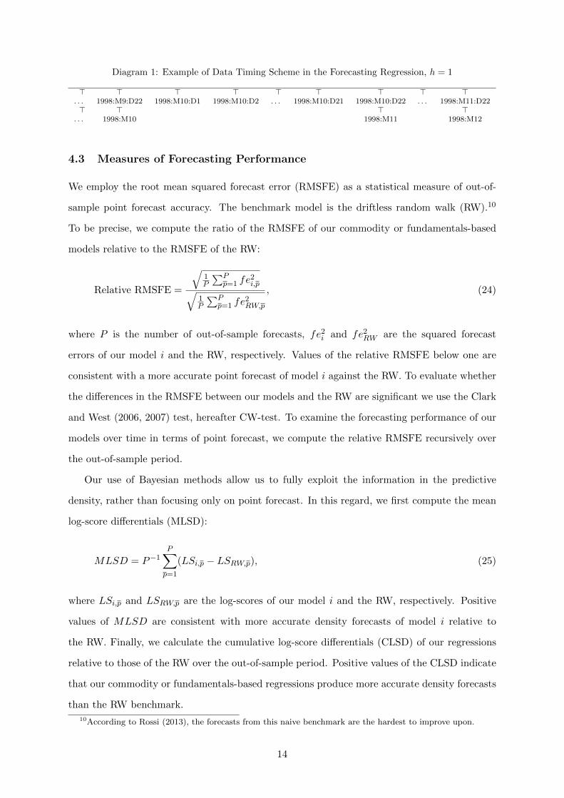
Diagram 1: Example of Data Timing Scheme in the Forecasting Regression, h = 1
> > > > > > > > >. . . 1998:M9:D22 1998:M10:D1 1998:M10:D2 . . . 1998:M10:D21 1998:M10:D22 . . . 1998:M11:D22> > > >
. . . 1998:M10 1998:M11 1998:M12
4.3 Measures of Forecasting Performance
We employ the root mean squared forecast error (RMSFE) as a statistical measure of out-of-
sample point forecast accuracy. The benchmark model is the driftless random walk (RW).10
To be precise, we compute the ratio of the RMSFE of our commodity or fundamentals-based
models relative to the RMSFE of the RW:
Relative RMSFE =
√1P
∑Pp=1 fe
2i,p√
1P
∑Pp=1 fe
2RW,p
, (24)
where P is the number of out-of-sample forecasts, fe2i and fe2RW are the squared forecast
errors of our model i and the RW, respectively. Values of the relative RMSFE below one are
consistent with a more accurate point forecast of model i against the RW. To evaluate whether
the differences in the RMSFE between our models and the RW are significant we use the Clark
and West (2006, 2007) test, hereafter CW-test. To examine the forecasting performance of our
models over time in terms of point forecast, we compute the relative RMSFE recursively over
the out-of-sample period.
Our use of Bayesian methods allow us to fully exploit the information in the predictive
density, rather than focusing only on point forecast. In this regard, we first compute the mean
log-score differentials (MLSD):
MLSD = P−1P∑p=1
(LSi,p − LSRW,p), (25)
where LSi,p and LSRW,p are the log-scores of our model i and the RW, respectively. Positive
values of MLSD are consistent with more accurate density forecasts of model i relative to
the RW. Finally, we calculate the cumulative log-score differentials (CLSD) of our regressions
relative to those of the RW over the out-of-sample period. Positive values of the CLSD indicate
that our commodity or fundamentals-based regressions produce more accurate density forecasts
than the RW benchmark.
10According to Rossi (2013), the forecasts from this naive benchmark are the hardest to improve upon.
14
5 Forecasting Performance: Empirical Results
5.1 Single Predictor Models
In Table 1 we assess the forecasting performance of models conditioned on each of the regressors
we consider. While in the left panel we focus on the relative RMSFE to examine performance
in terms of point forecast, in the right panel we look at log-score differentials to inspect density
forecast improvements. Focusing on point forecasts, models conditioned on daily regressors,
i.e. the MIDAS models, yield a lower RMSFE than the RW benchmark for some commodity-
currency pairs. This is the case for the Australian and Canadian dollar MIDAS regressions
with copper prices. For instance, for the Australian dollar and changes in copper prices the
MIDAS regression reduces the RMSFE by 1.1% relative to the benchmark. An improvement of
the same magnitude is also patent in the non-commodity currency we examine - the Japanese
Yen. While these reductions in the RMSFE are seemingly low, our tests of equal predictive
ability suggest that the differences in the RMSFE we detect are statistically significant. Later,
we will examine other metrics to gain more insights on the consistence of these gains over the
out-of-sample period.
Also using the RMSFE metric, regressions with monthly commodity prices fail to forecast
better than the RW benchmark, as in these cases the relative RMSFE are all above one. Hence,
in line with Ferraro et al. (2015) and Chen et al. (2010), we affirm the lack of predictive content
of commodity prices sampled at low frequency for monthly variations in exchange rates. As
well, our results support the prevalent view in the literature regarding the predictive ability of
fundamentals derived from Taylor rules. See, for instance, Molodtsova and Papell (2009) and
Rossi (2013). As shown in the table, among the standard macroeconomic fundamentals we use,
only those from the Taylor rule display a significant predictive content for at least one currency
- the Canadian dollar. In contrast, fundamentals from the Monetary Model (MM), PPP, and
UIP yield a relative RMSFE above one, with MM exhibiting the weakest performance for most
currency pairs.
Turning to density forecasts in the right panel, results reveal that once we account for the
entire forecast distribution, the RW never outperforms our commodity or fundamentals-based
regressions. In all cases, the log-score differentials are significantly positive, with MIDAS models
on certain commodity-currency pairs exhibiting the largest values. For example, the MIDAS
model with daily gold prices changes displays the largest log-score differentials among all the
15
forecasting models for the Australian dollar. A similar assertion holds for daily copper prices
and the Canadian dollar, as well as daily oil prices and the Norwegian Kroner.
On balance, we find that when we exploit the full predictive density, all the commodity
or fundamentals-based models provide more accurate forecasts than the RW benchmark. In
terms of point forecasts, daily commodity prices and Taylor rule fundamentals improve forecast
accuracy relative to the RW benchmark in several cases.11
5.2 Forecast Combinations
The results in the previous section are based on individual model performance and therefore
do not exploit the possibility that one regressor might have forecasted well in parts of the
out-of-sample period and poorly in other parts. To exploit this possibility and account for
time-variation in forecasting performance, we now turn to forecast combinations methods.
Table 2 reports results for forecast combinations under BMA, BMS, the optimal predictive
pool, and a simple average of all individual model’s forecasts. This latter case is equivalent
to assigning constant weights of 1/MN to each model’s forecast. We notice immediately the
benefits of forecast combinations, since in most cases we improve upon the benchmark. In the
case of the Australian dollar, for instance, either combining forecasts from daily regressors or,
both, daily and monthly predictors leads to better performance with all Bayesian combination
methods. For the Yen, instead, combining only daily regressors produces the best outcomes,
while for the Australian dollar the best results are achieved with monthly commodity prices
and macroeconomic fundamentals. In the case of the Norwegian Kroner/USD exchange rate,
we note the inability of either method to improve upon the RW, consistent with results from
the single predictor forecast evaluation.
Whilst the results show that combination methods based on time-varying weights are supe-
rior to the constant weighting scheme, among the former methods there is no clear ranking in
terms of the overall best method across currencies. When the forecasts from monthly regressors
are combined, the optimal predictive pool delivers the largest reduction in the relative RMSFE
for the Canadian dollar. But for Australian dollar and combination of daily regressors, BMS
achieves the best performance. In some instances, such as for the Yen with daily regressors,
both BMA and BMS perform equally well.
11In Appendix D we experiment with a 3-months forecasting horizon. Results are less favorable to either dailyor monthly commodity prices in terms of point forecasts. Results for density forecasts are comparable to thosewe find for 1-month horizon.
16
5.3 Forecasting Performance Over Time
All our results so far are based on measures of global performance since they are based on
averages over the out-of-sample (OOS) period. These metrics leave open the question of whether
they are influenced by a few data-points in the OOS period and if the performance we obtain
is consistent over the entire OOS period. To shed light on these questions, we next examine
metrics of local relative performance, namely the recursive relative RMSFE and the cumulative
log-score differentials.
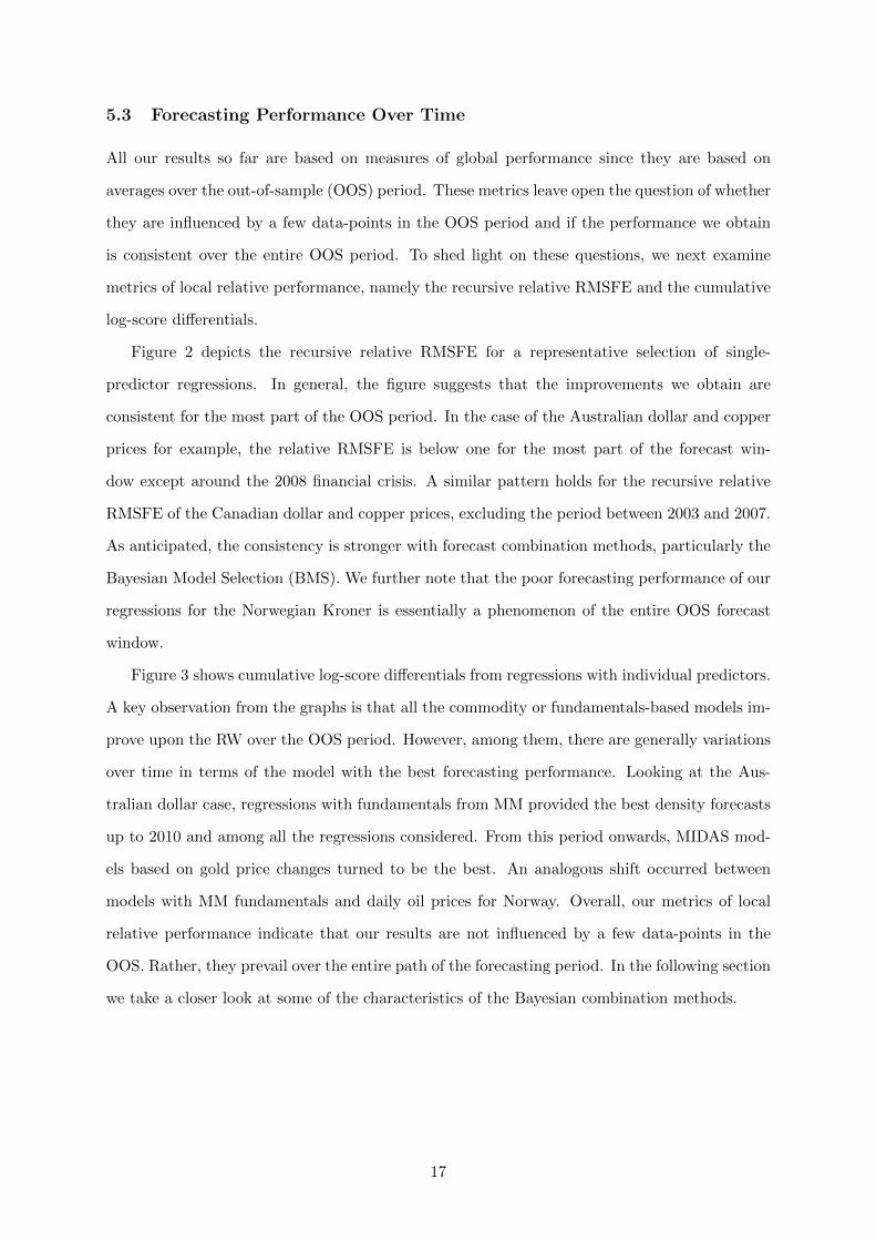
Figure 2 depicts the recursive relative RMSFE for a representative selection of single-
predictor regressions. In general, the figure suggests that the improvements we obtain are
consistent for the most part of the OOS period. In the case of the Australian dollar and copper
prices for example, the relative RMSFE is below one for the most part of the forecast win-
dow except around the 2008 financial crisis. A similar pattern holds for the recursive relative
RMSFE of the Canadian dollar and copper prices, excluding the period between 2003 and 2007.
As anticipated, the consistency is stronger with forecast combination methods, particularly the
Bayesian Model Selection (BMS). We further note that the poor forecasting performance of our
regressions for the Norwegian Kroner is essentially a phenomenon of the entire OOS forecast
window.
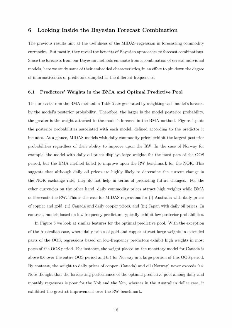
Figure 3 shows cumulative log-score differentials from regressions with individual predictors.
A key observation from the graphs is that all the commodity or fundamentals-based models im-
prove upon the RW over the OOS period. However, among them, there are generally variations
over time in terms of the model with the best forecasting performance. Looking at the Aus-
tralian dollar case, regressions with fundamentals from MM provided the best density forecasts
up to 2010 and among all the regressions considered. From this period onwards, MIDAS mod-
els based on gold price changes turned to be the best. An analogous shift occurred between
models with MM fundamentals and daily oil prices for Norway. Overall, our metrics of local
relative performance indicate that our results are not influenced by a few data-points in the
OOS. Rather, they prevail over the entire path of the forecasting period. In the following section
we take a closer look at some of the characteristics of the Bayesian combination methods.
17
6 Looking Inside the Bayesian Forecast Combination
The previous results hint at the usefulness of the MIDAS regression in forecasting commodity
currencies. But mostly, they reveal the benefits of Bayesian approaches to forecast combinations.
Since the forecasts from our Bayesian methods emanate from a combination of several individual
models, here we study some of their embedded characteristics, in an effort to pin down the degree
of informativeness of predictors sampled at the different frequencies.
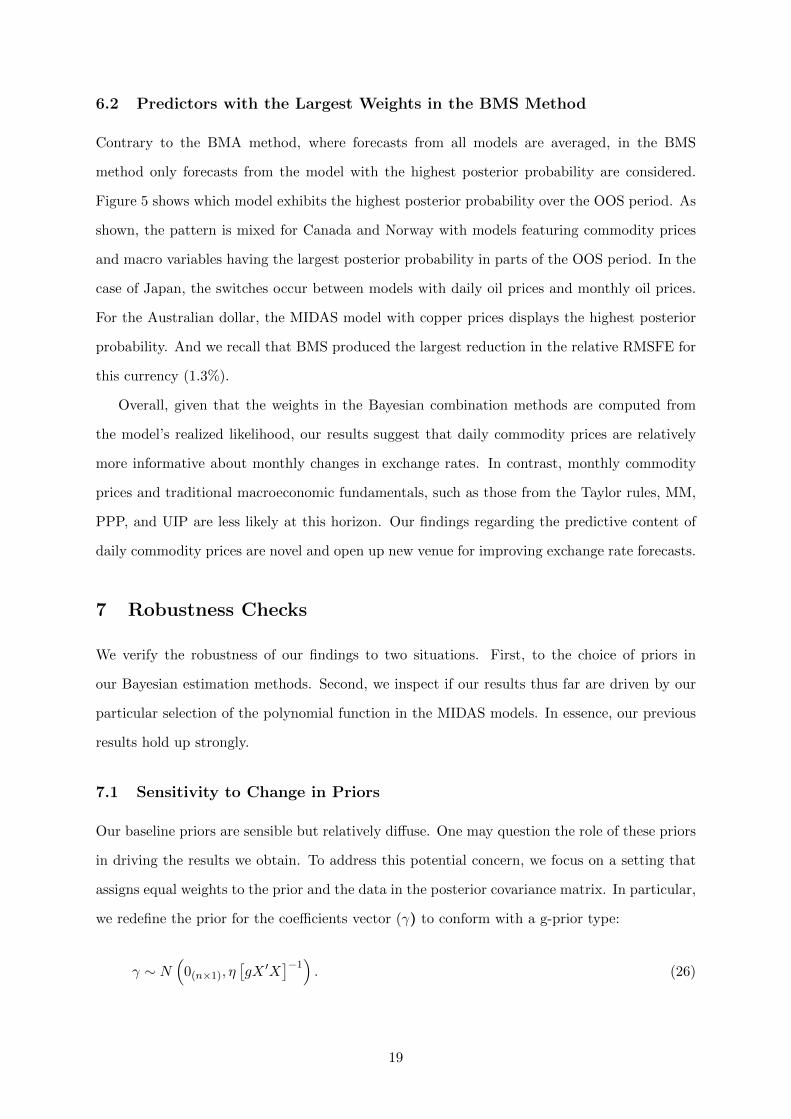
6.1 Predictors’ Weights in the BMA and Optimal Predictive Pool
The forecasts from the BMA method in Table 2 are generated by weighting each model’s forecast
by the model’s posterior probability. Therefore, the larger is the model posterior probability,
the greater is the weight attached to the model’s forecast in the BMA method. Figure 4 plots
the posterior probabilities associated with each model, defined according to the predictor it
includes. At a glance, MIDAS models with daily commodity prices exhibit the largest posterior
probabilities regardless of their ability to improve upon the RW. In the case of Norway for
example, the model with daily oil prices displays large weights for the most part of the OOS
period, but the BMA method failed to improve upon the RW benchmark for the NOK. This
suggests that although daily oil prices are highly likely to determine the current change in
the NOK exchange rate, they do not help in terms of predicting future changes. For the
other currencies on the other hand, daily commodity prices attract high weights while BMA
outforecasts the RW. This is the case for MIDAS regressions for (i) Australia with daily prices
of copper and gold, (ii) Canada and daily copper prices, and (iii) Japan with daily oil prices. In
contrast, models based on low frequency predictors typically exhibit low posterior probabilities.
In Figure 6 we look at similar features for the optimal predictive pool. With the exception
of the Australian case, where daily prices of gold and copper attract large weights in extended
parts of the OOS, regressions based on low-frequency predictors exhibit high weights in most
parts of the OOS period. For instance, the weight placed on the monetary model for Canada is
above 0.6 over the entire OOS period and 0.4 for Norway in a large portion of this OOS period.
By contrast, the weight to daily prices of copper (Canada) and oil (Norway) never exceeds 0.4.
Note thought that the forecasting performance of the optimal predictive pool among daily and
monthly regressors is poor for the Nok and the Yen, whereas in the Australian dollar case, it
exhibited the greatest improvement over the RW benchmark.
18
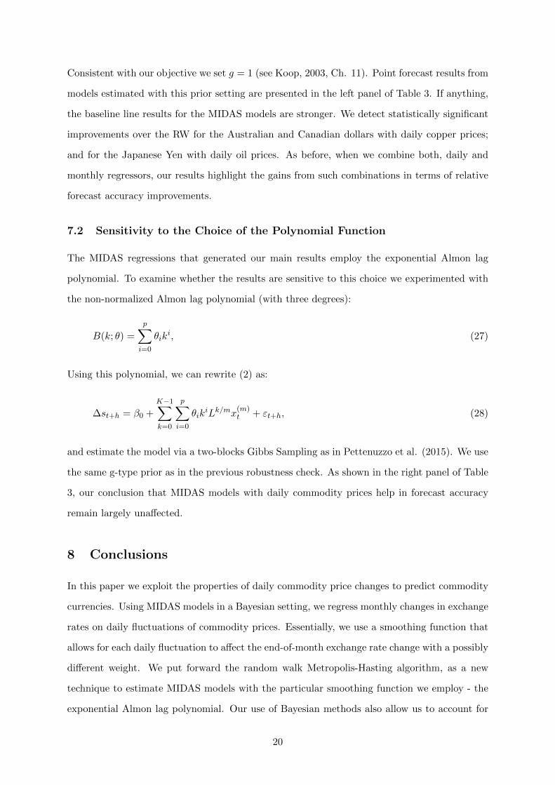
6.2 Predictors with the Largest Weights in the BMS Method
Contrary to the BMA method, where forecasts from all models are averaged, in the BMS
method only forecasts from the model with the highest posterior probability are considered.
Figure 5 shows which model exhibits the highest posterior probability over the OOS period. As
shown, the pattern is mixed for Canada and Norway with models featuring commodity prices
and macro variables having the largest posterior probability in parts of the OOS period. In the
case of Japan, the switches occur between models with daily oil prices and monthly oil prices.
For the Australian dollar, the MIDAS model with copper prices displays the highest posterior
probability. And we recall that BMS produced the largest reduction in the relative RMSFE for
this currency (1.3%).
Overall, given that the weights in the Bayesian combination methods are computed from
the model’s realized likelihood, our results suggest that daily commodity prices are relatively
more informative about monthly changes in exchange rates. In contrast, monthly commodity
prices and traditional macroeconomic fundamentals, such as those from the Taylor rules, MM,
PPP, and UIP are less likely at this horizon. Our findings regarding the predictive content of
daily commodity prices are novel and open up new venue for improving exchange rate forecasts.
7 Robustness Checks
We verify the robustness of our findings to two situations. First, to the choice of priors in
our Bayesian estimation methods. Second, we inspect if our results thus far are driven by our
particular selection of the polynomial function in the MIDAS models. In essence, our previous
results hold up strongly.
7.1 Sensitivity to Change in Priors
Our baseline priors are sensible but relatively diffuse. One may question the role of these priors
in driving the results we obtain. To address this potential concern, we focus on a setting that
assigns equal weights to the prior and the data in the posterior covariance matrix. In particular,
we redefine the prior for the coefficients vector (γ) to conform with a g-prior type:
γ ∼ N(
0(n×1), η[gX ′X
]−1). (26)
19
Consistent with our objective we set g = 1 (see Koop, 2003, Ch. 11). Point forecast results from
models estimated with this prior setting are presented in the left panel of Table 3. If anything,
the baseline line results for the MIDAS models are stronger. We detect statistically significant
improvements over the RW for the Australian and Canadian dollars with daily copper prices;
and for the Japanese Yen with daily oil prices. As before, when we combine both, daily and
monthly regressors, our results highlight the gains from such combinations in terms of relative
forecast accuracy improvements.
7.2 Sensitivity to the Choice of the Polynomial Function
The MIDAS regressions that generated our main results employ the exponential Almon lag
polynomial. To examine whether the results are sensitive to this choice we experimented with
the non-normalized Almon lag polynomial (with three degrees):
B(k; θ) =
p∑i=0
θiki, (27)
Using this polynomial, we can rewrite (2) as:
∆st+h = β0 +K−1∑k=0
p∑i=0
θikiLk/mx
(m)t + εt+h, (28)
and estimate the model via a two-blocks Gibbs Sampling as in Pettenuzzo et al. (2015). We use
the same g-type prior as in the previous robustness check. As shown in the right panel of Table
3, our conclusion that MIDAS models with daily commodity prices help in forecast accuracy
remain largely unaffected.
8 Conclusions
In this paper we exploit the properties of daily commodity price changes to predict commodity
currencies. Using MIDAS models in a Bayesian setting, we regress monthly changes in exchange
rates on daily fluctuations of commodity prices. Essentially, we use a smoothing function that
allows for each daily fluctuation to affect the end-of-month exchange rate change with a possibly
different weight. We put forward the random walk Metropolis-Hasting algorithm, as a new
technique to estimate MIDAS models with the particular smoothing function we employ - the
exponential Almon lag polynomial. Our use of Bayesian methods also allow us to account for
20

potential instabilities in forecasting performance and examine the degree of informativeness of
the daily commodity price changes, as opposed to the monthly commodity prices and standard
macroeconomic fundamentals.
Focusing on data for Australia, Canada, Norway, and Japan we first find evidence favouring
daily commodity prices fluctuations in terms of providing more accurate forecasts than the naive
no-change benchmark. In particular, daily changes in copper prices yield point forecast improve-
ments for the Australian and Canadian dollar at the 1-month horizon we consider. In addition,
we detect significant predictive content of daily oil prices changes for the non-commodity cur-
rency we examine, the Japanese Yen. In contrast and as reported in other studies, we identify
rare instances in which monthly commodity prices changes lead to systematic point forecast
improvements. However, consistent with the existing evidence, macroeconomic fundamentals
derived from Taylor rules do exhibit predictive power for some commodity currencies.
We then proceed and combine forecasts from regressions based on daily and monthly com-
modity prices and monthly traditional macroeconomic fundamentals, in an effort to account
for time-variation in forecasting ability of our predictors. Here our empirical findings reveal
the usefulness of such combinations in terms of forecast accuracy improvements relative to our
benchmark. Our results also hint at the importance of accounting for the full forecast distribu-
tion, since in terms of density forecasts, our predictions are always better than those from the
RW. Finally, when we inspect the weights underlying our forecast combinations approaches we
find that daily commodity prices are relatively more informative about 1-month changes in the
exchange rate than monthly commodity prices or the typical macroeconomic variables.
Overall, we interpret our results as endorsing the view that the key to establishing predictive
content of daily commodity prices for exchange rates, hinges upon exploiting their short-lived
content in a MIDAS setup.
21
References
Andreou, E., E. Ghysels, and A. Kourtellos (2010). Regression models with mixed sampling
frequencies. Journal of Econometrics 158 (2), 246–261.
Bacchetta, P. and E. V. Wincoop (2004). A scapegoat model of exchange-rate fluctuations.
American Economic Review 94 (2), 114–118.
Bacchetta, P. and E. V. Wincoop (2013). On the unstable relationship between exchange rates
and macroeconomic fundamentals. Journal of International Economics 91 (1), 18–26.
Berge, T. J. (2013). Forecasting disconnected exchange rates. Journal of Applied Economet-
rics 29 (5), 713–735.
Chen, Y.-C., K. S. Rogoff, and B. Rossi (2010). Can exchange rates forecast commodity
prices? The Quarterly Journal of Economics 125 (3), 1145–1194.
Clark, T. E. and K. D. West (2006). Using out-of-sample mean squared prediction errors to
test the martingale difference hypothesis. Journal of Econometrics 135 (1), 155–186.
Clark, T. E. and K. D. West (2007). Approximately normal tests for equal predictive accuracy
in nested models. Journal of Econometrics 138 (1), 291–311.
Engel, C. and K. D. West (2005). Exchange rates and fundamentals. Journal of Political
Economy 113 (3), 485–517.
Ferraro, D., K. Rogoff, and B. Rossi (2015). Can oil prices forecast exchange rates? An em-
pirical analysis of the relationship between commodity prices and exchange rates. Journal
of International Money and Finance 54 (0), 116 – 141.
Foroni, C., M. Marcellino, and C. Schumacher (2013). Unrestricted mixed data sampling
(MIDAS): MIDAS regressions with unrestricted lag polynomials. Journal of the Royal
Statistical Society: Series A (Statistics in Society) 178 (1), 57–82.
Fratzscher, M., D. Rime, L. Sarno, and G. Zinna (2015). The scapegoat theory of exchange
rates: the first tests. Journal of Monetary Economics 70, 1 – 21.
Gelfand, A. E. and D. K. Dey (1994). Bayesian model choice: asymptotics and exact calcula-
tions. Journal of the Royal Statistical Society. Series B (Methodological) 56 (3), 501–514.
Geweke, J. (1992). Evaluating the accuracy of sampling-based approaches to the calculation
of posterior moments. Bayesian Statistics 4, 169–194.
22
Geweke, J. and G. Amisano (2011). Optimal prediction pools. Journal of Economet-
rics 164 (1), 130 – 141. Annals Issue on Forecasting.
Ghysels, E., P. Santa-Clara, and R. Valkanov (2005). There is a risk-return trade-off after
all. Journal of Financial Economics 76 (3), 509–548.
Ghysels, E., A. Sinko, and R. Valkanov (2007). Midas regressions: further results and new
directions. Econometric Reviews 26 (1), 53–90.
Giacomini, R. and B. Rossi (2010). Forecast comparisons in unstable environments. Journal
of Applied Econometrics 25 (4), 595–620.
Hodrick, R. J. and E. C. Prescott (1997). Postwar us business cycles: an empirical investiga-
tion. Journal of Money, Credit and Banking 29 (1), 1–16.
Koop, G. (2003). Bayesian econometrics. London: John Wiley & Sons, Ltd.
Marcellino, M., J. Stock, and M. Watson (2006). A comparison of direct and iterated multistep
ar methods for forecasting macroeconomic time series. Journal of Econometrics 135, 499–
526.
Mark, N. C. (1995). Exchange rates and fundamentals: evidence on long-horizon predictabil-
ity. The American Economic Review 85 (1), 201–218.
Meese, R. A. and K. Rogoff (1983). Empirical exchange rate models of the seventies: do they
fit out of sample? Journal of International Economics 14 (1), 3–24.
Mitchell, J. and S. G. Hall (2005). Evaluating, comparing and combining density forecasts
using the KLIC with an application to the Bank of England and NIESER fan charts of
inflation. Oxford Bulletin of Economics and Statistics 67, 995–1033.
Molodtsova, T. and D. H. Papell (2009). Out-of-sample exchange rate predictability with
taylor rule fundamentals. Journal of International Economics 77 (2), 167–180.
Pettenuzzo, D., A. G. Timmermann, and R. I. Valkanov (2015). A Bayesian midas approach
to modeling first and second moment dynamics. Technical Report CEPR Discussion Paper
No. DP10160.
Rogoff, K. S. and V. Stavrakeva (2008). The continuing puzzle of short horizon exchange rate
forecasting. NBER Working Paper 14071, National Bureau of Economic Research.
Rossi, B. (2013). Exchange rate predictability. Journal of Economic Literature 51 (4), 1063–
1119.
23

Sarno, L. and G. Valente (2009). Exchange rates and fundamentals: footloose or evolving
relationship? Journal of the European Economic Association 7 (4), 786–830.
Watson, M. W. (2007). How accurate are real-time estimates of output trends and gaps?
Economic Quarterly 93 (2), 143–161.
Wright, J. H. (2008). Bayesian model averaging and exchange rate forecasts. Journal of
Econometrics 146 (2), 329–341.
24
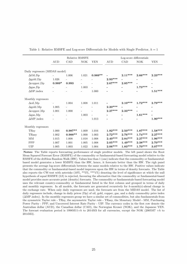
Table 1: Relative RMSFE and Log-score Differentials for Models with Single Predictor, h = 1
Relative RMSFE Log-score differentials
AUD CAD NOK YEN AUD CAD NOK YEN
Daily regressors (MIDAS model)
∆Oil Dp - 1.006 1.021 0.989** - 2.11*** 2.66*** 2.23***
∆gold Dp 1.026 - - - 2.93*** - - -
∆copper Dp 0.989* 0.993 - - 2.67*** 2.85*** - -
∆gas Dp - - 1.003 - - - 1.73*** -
∆DP index - - - 1.000 - - - 1.51***
Monthly regressors
∆oil Mp - 1.004 1.008 1.011 - 2.10*** 1.72*** 2.79***
∆gold Mp 1.005 - - - 2.20*** - - -
∆copper Mp 1.001 1.000 - - 2.27*** 2.33*** - -
∆gas Mp - - 1.003 - - - 1.61*** -
∆MP index - - - 1.013 - - - 1.90***
Monthly regressors
TRsy 1.000 0.987** 1.009 1.016 1.92*** 2.50*** 1.87*** 1.58***
TRasy 1.002 0.988** 1.000 1.003 2.72*** 2.76*** 1.74*** 2.27***
MM 1.015 1.008 1.018 1.008 2.40*** 2.84*** 2.27*** 1.96***
PPP 1.007 1.001 1.005 1.008 2.05*** 1.49*** 2.38*** 2.70***
UIP 1.005 1.003 1.022 1.004 2.06*** 1.83*** 1.70*** 3.07***
Notes: The Table reports forecasting performance of single preditor models. The left panel shows the RootMean Squared Forecast Error (RMSFE) of the commodity or fundamental-based forecasting model relative to theRMSFE of the driftless Random Walk (RW). Values less than 1 (one) indicate that the commodity or fundamental-based model generates a lower RMSFE than the RW, hence, it forecasts better than the RW. The righ panelpresents the average log-score differentials between the same models relative to the RW. Positive values indicatethat the commodity or fundamental-based model improves upon the RW in terms of density forecasts. The Tablealso reports the CW-test with asterisks (10%, **5%, ***1%) denoting the level of significance at which the nullhypothesis of equal RMSFE (LS) is rejected, favouring the alternative that the commodity or fundamental-basedmodel provides more accurate point (density) forecasts. The commodity or fundamentals-based forecasting modeluses the relevant country-commodity or fundamental listed in the first column and grouped in terms of dailyand monthly regressors. In all models, the forecasts are generated recursively for h-month(s)-ahead change inthe exchange rate. When only daily regressors are used, the forecasts are from the MIDAS model. The list ofdaily regressors include, change in daily prices (Dp) of oil, gold, copper, gas, and a daily commodity price index(∆MP index). In the monthly regressors group we have a similar set of commodities, but also fundamentals fromthe symmetric Taylor rule - TRsy, the asymmetric Taylor rule - TRasy, the Monetary Model - MM, PurchasingPower Parity - PPP, and Uncovered Interest Rate Parity - UIP. The currency codes in the first row denote theAustralian dollar (AUD), the Canadian dollar (CAD), the Norwegian Kroner (NOK), and the Japanese YEN.The forecast evaluation period is 1998M11+h to 2014M3 for all currencies, except the NOK (2005M7 +h to2014M3).
25

Table 2: Relative RMSFE and CW-test for Forecast Combinations, h = 1
Daily regressors -Commodity Prices(CmdtyP)
Monthly regressors (Cmd-tyP and macro fundamen-tals)
Daily and monthly regres-sors (CmdtyP and macrofundamentals)
BMA BMS BMA BMS BMA BMS
AUD 0.992 0.987* 1.002 1.000 0.993 0.987*
CAD 1.000 0.999 0.991** 0.995* 0.996 0.998
NOK 1.014 1.016 1.009 1.005 1.019 1.017
YEN 0.989** 0.989** 1.004 1.003 0.998 0.999
OptPool EqWeights OptPool EqWeights OptPool EqWeights
AUD 0.990* 1.000 1.013 1.002 0.990* 1.000
CAD 1.002 1.002 0.990** 0.997 0.996 0.997
NOK 1.019 1.007 1.029 1.008 1.036 1.007
YEN 0.990** 0.995* 1.011 1.003 1.009 1.001
Notes: The table reports the Root Mean Squared Forecast Error (RMSFE) for forecast combination methodsrelative to the RMSFE of the driftless Random Walk (RW). The methods include, Bayesian Model Averaging(BMA), Bayesian Model Selection, (BMS), the Optimal Predictive Pool (OptPool) of Geweke and Amisano(2011), and a simple equal-weighting scheme (EqWeights). Values less than 1 (one) indicate that the combinationmethod generates a lower RMSFE than the RW, hence, it forecasts better than the RW. The table also reportsthe CW-test with asterisks (10%, **5%, ***1%) denoting the level of significance at which the null hypothesisof equal RMSFE is rejected, favouring the alternative that the combination method has a lower RMSFE. Theforecast combinations are based on the relevant commodity-currency and standard macroeconomic fundamentals.For the Australian dollar (AUD) the relevant commodities are gold and copper; for the Canadian dollar (CAD)- oil and copper; and for the Norwegian Kroner (NOK) these include oil and gas. When only daily regressors areused the combination is based on forecasts from the MIDAS models - reported in columns [2-3]. In columns [4-5]the combination is based on forecasts from monthly regressors, while the last two columns report results fromcombining daily and monthly regressors. In all cases, the forecasts are generated recursively for h-month(s)-aheadchange in the exchange rate. In the group of monthly regressors we have a set of commodity pairs similar to thedaily group, but also fundamentals from the symmetric Taylor rule - TRsy, the asymmetric Taylor rule - TRasy,the Monetary Model - MM, Purchasing Power Parity - PPP, and Uncovered Interest Rate Parity - UIP. Theforecast evaluation period is 1998M11+h to 2014M3 for all currencies, except the NOK (2005M7 +h to 2014M3).
26
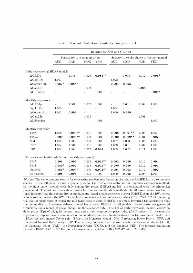
Table 3: Forecast Evaluation Sensitivity Analysis, h = 1
Relative RMSFE and CW-test
Sensitivity to change in priors Sensitivity to the choice of the polynomial
AUD CAD NOK YEN AUD CAD NOK YEN
Daily regressors (MIDAS model)
∆Oil Dp - 1.011 1.026 0.983** - 1.005 1.012 0.991*
∆Gold Dp 1.007 - - - 1.022 - - -
∆Copper Dp 0.987* 0.988* - - 0.994 0.993 - -
∆Gas Dp - - 1.002 - - - 0.995 -
∆DP index - - - 1.003 - - - 0.994*
Monthly regressors
∆Oil Mp - 1.001 1.002 1.002 - 1.001 1.004 1.002
∆gold Mp 1.003 - - - 1.004 - - -
∆Copper Mp 1.001 0.999 - - 1.000 0.999 - -
∆Gas Mp - - 1.003 - - - 1.001 -
∆MP index - - - 1.002 - - - 1.001
Monthly regressors
TRsy 1.000 0.993** 1.007 1.006 0.998 0.991** 1.005 1.007
TRasy 0.999 0.993** 1.000 1.001 0.999 0.992** 1.001 0.997
MM 1.005 1.003 1.006 1.003 1.007 1.003 1.009 1.000
PPP 1.004 1.001 1.001 1.000 1.003 1.001 1.002 1.001
UIP 1.001 1.003 1.012 0.998 1.003 1.002 1.011 1.002
Forecast combination (daily and monthly regressors)
BMA 0.991 0.993 1.015 0.991** 0.992 0.996 1.019 0.994
BMS 0.989* 0.994 1.013 0.991** 0.990 0.996 1.017 0.994
OptPool 0.986* 0.990* 1.030 0.992** 0.994 0.993 1.012 0.992
EqWeights 0.998 0.998 1.005 1.000 1.000 0.998 1.003 1.000
Notes: The table presents results for forecasting performance based on the relative RMSFE for two robustnesschecks. In the left panel we use a g-type prior for the coefficients vector in our Bayesian estimation method.In the right panel, models with daily commodity prices (MIDAS models) are estimated with the Almon lagpolynomial. The last four rows show results for forecast combination methods. In all cases, values less than 1(one) indicate that the commodity or fundamental-based model generates a lower RMSFE than the RW, hence,it forecasts better than the RW. The table also reports the CW-test with asterisks (10%, **5%, ***1%) denotingthe level of significance at which the null hypothesis of equal RMSFE is rejected, favouring the alternative thatthe commodity or fundamental-based model has a lower RMSFE. In all models, the forecasts are generatedrecursively for h-month(s)-ahead change in the exchange rate. The list of daily regressors include, change indaily prices (Dp) of oil, gold, copper, gas, and a daily commodity price index (∆MP index). In the monthlyregressors group we have a similar set of commodities, but also fundamentals from the symmetric Taylor rule- TRsy, the asymmetric Taylor rule - TRasy, the Monetary Model - MM, Purchasing Power Parity - PPP, andUncovered Interest Rate Parity - UIP. The currency codes in the first row denote the Australian dollar (AUD),the Canadian dollar (CAD), the Norwegian Kroner (NOK), and the Japanese YEN. The forecast evaluationperiod is 1998M11+h to 2014M3 for all currencies, except the NOK (2005M7 +h to 2014M3).
27
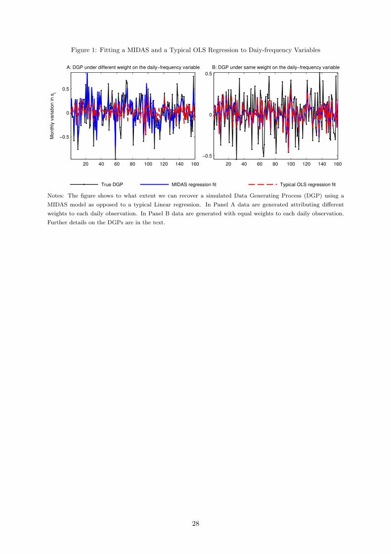
Figure 1: Fitting a MIDAS and a Typical OLS Regression to Daiy-frequency Variables
20 40 60 80 100 120 140 160
−0.5
0
0.5
A: DGP under different weight on the daily−frequency variable
Month
ly v
ariation in s
t
20 40 60 80 100 120 140 160
−0.5
0
0.5
B: DGP under same weight on the daily−frequency variable
True DGP MIDAS regression fit Typical OLS regression fit
Notes: The figure shows to what extent we can recover a simulated Data Generating Process (DGP) using a
MIDAS model as opposed to a typical Linear regression. In Panel A data are generated attributing different
weights to each daily observation. In Panel B data are generated with equal weights to each daily observation.
Further details on the DGPs are in the text.
28
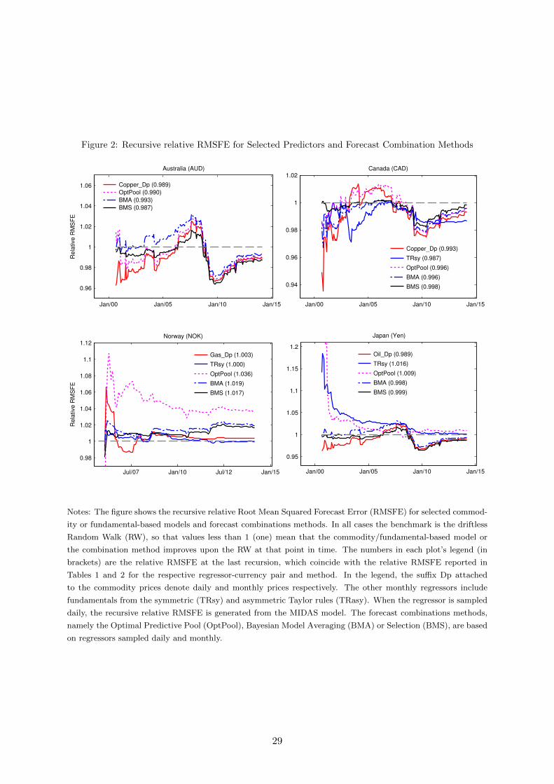
Figure 2: Recursive relative RMSFE for Selected Predictors and Forecast Combination Methods
Jan/00 Jan/05 Jan/10 Jan/15
0.96
0.98
1
1.02
1.04
1.06
Australia (AUD)
Rela
tive R
MS
FE
Copper_Dp (0.989)
OptPool (0.990)
BMA (0.993)
BMS (0.987)
Jan/00 Jan/05 Jan/10 Jan/15
0.94
0.96
0.98
1
1.02Canada (CAD)
Copper_Dp (0.993)
TRsy (0.987)
OptPool (0.996)
BMA (0.996)
BMS (0.998)
Jul/07 Jan/10 Jul/12 Jan/15
0.98
1
1.02
1.04
1.06
1.08
1.1
1.12Norway (NOK)
Rela
tive R
MS
FE
Gas_Dp (1.003)
TRsy (1.000)
OptPool (1.036)
BMA (1.019)
BMS (1.017)
Jan/00 Jan/05 Jan/10 Jan/15
0.95
1
1.05
1.1
1.15
1.2
Japan (Yen)
Oil_Dp (0.989)
TRsy (1.016)
OptPool (1.009)
BMA (0.998)
BMS (0.999)
Notes: The figure shows the recursive relative Root Mean Squared Forecast Error (RMSFE) for selected commod-
ity or fundamental-based models and forecast combinations methods. In all cases the benchmark is the driftless
Random Walk (RW), so that values less than 1 (one) mean that the commodity/fundamental-based model or
the combination method improves upon the RW at that point in time. The numbers in each plot’s legend (in
brackets) are the relative RMSFE at the last recursion, which coincide with the relative RMSFE reported in
Tables 1 and 2 for the respective regressor-currency pair and method. In the legend, the suffix Dp attached
to the commodity prices denote daily and monthly prices respectively. The other monthly regressors include
fundamentals from the symmetric (TRsy) and asymmetric Taylor rules (TRasy). When the regressor is sampled
daily, the recursive relative RMSFE is generated from the MIDAS model. The forecast combinations methods,
namely the Optimal Predictive Pool (OptPool), Bayesian Model Averaging (BMA) or Selection (BMS), are based
on regressors sampled daily and monthly.
29
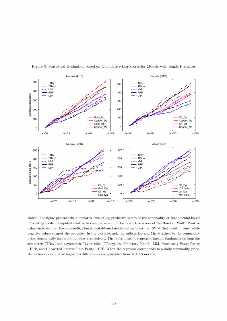
Figure 3: Statistical Evaluation based on Cumulative Log-Scores for Models with Single Predictor
Jan/00 Jan/05 Jan/10 Jan/15
0
100
200
300
400
500
Australia (AUD)
cum
ula
tive log s
core
Gold_Dp
Copper_Dp
Gold_Mp
Copper_Mp
TRsy
TRasy
MM
PPP
UIP
Jan/00 Jan/05 Jan/10 Jan/15
0
100
200
300
400
500
Canada (CAD)
Oil_Dp
Copper_Dp
Oil_Mp
Copper_Mp
TRsy
TRasy
MM
PPP
UIP
Jul/07 Jan/10 Jul/12 Jan/15
0
50
100
150
200
250
Norway (NOK)
cum
ula
tive log s
core
Oil_Dp
Gas_Dp
Oil_Mp
Gas_Mp
TRsy
TRasy
MM
PPP
UIP
Jan/00 Jan/05 Jan/10 Jan/15
0
100
200
300
400
500
Japan (Yen)
Oil_Dp
�DP_index
Oil_Mp
MP_index
TRsy
TRasy
MM
PPP
UIP
Notes: The figure presents the cumulative sum of log predictive scores of the commodity or fundamental-based
forecasting model, computed relative to cumulative sum of log predictive scores of the Random Walk. Positive
values indicate that the commodity/fundamental-based model outperforms the RW at that point in time, while
negative values suggest the opposite. In the plot’s legend, the suffixes Dp and Mp attached to the commodity
prices denote daily and monthly prices respectively. The other monthly regressors include fundamentals from the
symmetric (TRsy) and asymmetric Taylor rules (TRasy), the Monetary Model - MM, Purchasing Power Parity
- PPP, and Uncovered Interest Rate Parity - UIP. When the regressor corresponds to a daily commodity price,
the recursive cumulative log-scores differentials are generated from MIDAS models.
30
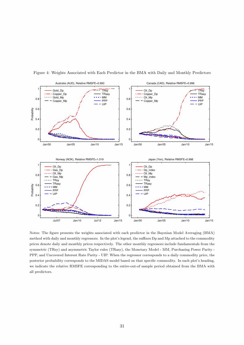
Figure 4: Weights Associated with Each Predictor in the BMA with Daily and Monthly Predictors
Jan/00 Jan/05 Jan/10 Jan/15
0
0.2
0.4
0.6
0.8
1
Pro
babili
ty
Australia (AUD), Relative RMSFE=0.993
Gold_Dp
Copper_Dp
Gold_Mp
Copper_Mp
TRsy
TRasy
MM
PPP
UIP
Jan/00 Jan/05 Jan/10 Jan/15
0
0.2
0.4
0.6
0.8
1
Canada (CAD), Relative RMSFE=0.996
Oil_Dp
Copper_Dp
Oil_Mp
Copper_Mp
TRsy
TRasy
MM
PPP
UIP
Jul/07 Jan/10 Jul/12 Jan/15
0
0.2
0.4
0.6
0.8
1
Pro
babili
ty
Norway (NOK), Relative RMSFE=1.019
Oil_Dp
Gas_Dp
Oil_Mp
Gas_Mp
TRsy
TRasy
MM
PPP
UIP
Jan/00 Jan/05 Jan/10 Jan/15
0
0.2
0.4
0.6
0.8
1
Japan (Yen), Relative RMSFE=0.998
Oil_Dp
Dp_index
Oil_Mp
Mp_index
TRsy
TRasy
MM
PPP
UIP
Notes: The figure presents the weights associated with each predictor in the Bayesian Model Averaging (BMA)
method with daily and monthly regressors. In the plot’s legend, the suffixes Dp and Mp attached to the commodity
prices denote daily and monthly prices respectively. The other monthly regressors include fundamentals from the
symmetric (TRsy) and asymmetric Taylor rules (TRasy), the Monetary Model - MM, Purchasing Power Parity -
PPP, and Uncovered Interest Rate Parity - UIP. When the regressor corresponds to a daily commodity price, the
posterior probability corresponds to the MIDAS model based on that specific commodity. In each plot’s heading,
we indicate the relative RMSFE corresponding to the entire-out-of sample period obtained from the BMA with
all predictors.
31
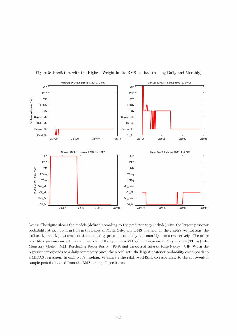
Figure 5: Predictors with the Highest Weight in the BMS method (Among Daily and Monthly)
Jan/00 Jan/05 Jan/10 Jan/15
Gold_Dp
Copper_Dp
Gold_Mp
Copper_Mp
TRsy
TRasy
MM
PPP
UIP
Australia (AUD), Relative RMSFE=0.987
Pre
dic
tor
with
ma
x P
rob
.
Jan/00 Jan/05 Jan/10 Jan/15
Oil_Dp
Copper_Dp
Oil_Mp
Copper_Mp
TRsy
TRasy
MM
PPP
UIP
Canada (CAD), Relative RMSFE=0.998
Jul/07 Jan/10 Jul/12 Jan/15
Oil_Dp
Gas_Dp
Oil_Mp
Gas_Mp
TRsy
TRasy
MM
PPP
UIP
Norway (NOK), Relative RMSFE=1.017
Pre
dic
tor
with
ma
x P
rob
.
Jan/00 Jan/05 Jan/10 Jan/15
Oil_Dp
Dp_index
Oil_Mp
Mp_index
TRsy
TRasy
MM
PPP
UIP
Japan (Yen), Relative RMSFE=0.999
Notes: The figure shows the models (defined according to the predictor they include) with the largest posterior
probability at each point in time in the Bayesian Model Selection (BMS) method. In the graph’s vertical axis, the
suffixes Dp and Mp attached to the commodity prices denote daily and monthly prices respectively. The other
monthly regressors include fundamentals from the symmetric (TRsy) and asymmetric Taylor rules (TRasy), the
Monetary Model - MM, Purchasing Power Parity - PPP, and Uncovered Interest Rate Parity - UIP. When the
regressor corresponds to a daily commodity price, the model with the largest posterior probability corresponds to
a MIDAS regression. In each plot’s heading, we indicate the relative RMSFE corresponding to the entire-out-of
sample period obtained from the BMS among all predictors.
32
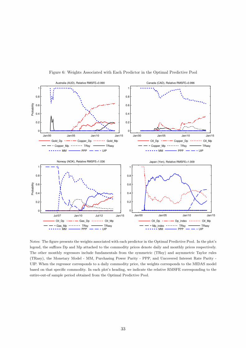
Figure 6: Weights Associated with Each Predictor in the Optimal Predictive Pool
Jan/00 Jan/05 Jan/10 Jan/15
0
0.2
0.4
0.6
0.8
1
Pro
ba
bili
ty
Australia (AUD), Relative RMSFE=0.990
Gold_Dp Copper_Dp Gold_Mp
Copper_Mp TRsy TRasy
MM PPP UIP
Jan/00 Jan/05 Jan/10 Jan/15
0
0.2
0.4
0.6
0.8
1
Canada (CAD), Relative RMSFE=0.996
Oil_Dp Copper_Dp Oil_Mp
Copper_Mp TRsy TRasy
MM PPP UIP
Jul/07 Jan/10 Jul/12 Jan/15
0
0.2
0.4
0.6
0.8
1
Pro
ba
bili
ty
Norway (NOK), Relative RMSFE=1.036
Oil_Dp Gas_Dp Oil_Mp
Gas_Mp TRsy TRasy
MM PPP UIP
Jan/00 Jan/05 Jan/10 Jan/15
0
0.2
0.4
0.6
0.8
1
Japan (Yen), Relative RMSFE=1.009
Oil_Dp Dp_index Oil_Mp
Mp_index TRsy TRasy
MM PPP UIP
Notes: The figure presents the weights associated with each predictor in the Optimal Predictive Pool. In the plot’s
legend, the suffixes Dp and Mp attached to the commodity prices denote daily and monthly prices respectively.
The other monthly regressors include fundamentals from the symmetric (TRsy) and asymmetric Taylor rules
(TRasy), the Monetary Model - MM, Purchasing Power Parity - PPP, and Uncovered Interest Rate Parity -
UIP. When the regressor corresponds to a daily commodity price, the weights corresponds to the MIDAS model
based on that specific commodity. In each plot’s heading, we indicate the relative RMSFE corresponding to the
entire-out-of sample period obtained from the Optimal Predictive Pool.
33
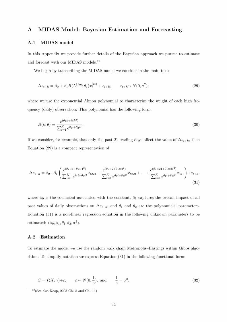
A MIDAS Model: Bayesian Estimation and Forecasting
A.1 MIDAS model
In this Appendix we provide further details of the Bayesian approach we pursue to estimate
and forecast with our MIDAS models.12
We begin by transcribing the MIDAS model we consider in the main text:
∆st+h = β0 + β1B(L1/m; θ1)x(m)t + εt+h, εt+h∼ N(0, σ2); (29)
where we use the exponential Almon polynomial to characterize the weight of each high fre-
quency (daily) observation. This polynomial has the following form:
B(k; θ) =e(θ1k+θ2k
2)∑Ki=1 e
θ1i+θ2i2. (30)
If we consider, for example, that only the past 21 trading days affect the value of ∆st+h, then
Equation (29) is a compact representation of:
∆st+h = β0+β1
(e(θ1×1+θ2×1
2)∑Ki=1 e
θ1i+θ2i2xtd21 +
e(θ1×2+θ2×22)∑K
i=1 eθ1i+θ2i2
xtd20 + ...+e(θ1×21+θ2×21
2)∑Ki=1 e
θ1i+θ2i2xtd1
)+εt+h.
(31)
where β0 is the coefficient associated with the constant, β1 captures the overall impact of all
past values of daily observations on ∆st+h, and θ1 and θ2 are the polynomials’ parameters.
Equation (31) is a non-linear regression equation in the following unknown parameters to be
estimated: (β0, β1, θ1, θ2, σ2).
A.2 Estimation
To estimate the model we use the random walk chain Metropolis–Hastings within Gibbs algo-
rithm. To simplify notation we express Equation (31) in the following functional form:
S = f(X, γ)+ε, ε ∼ N(0,1
η), and
1
η= σ2. (32)
12(See also Koop, 2003 Ch. 5 and Ch. 11)
34
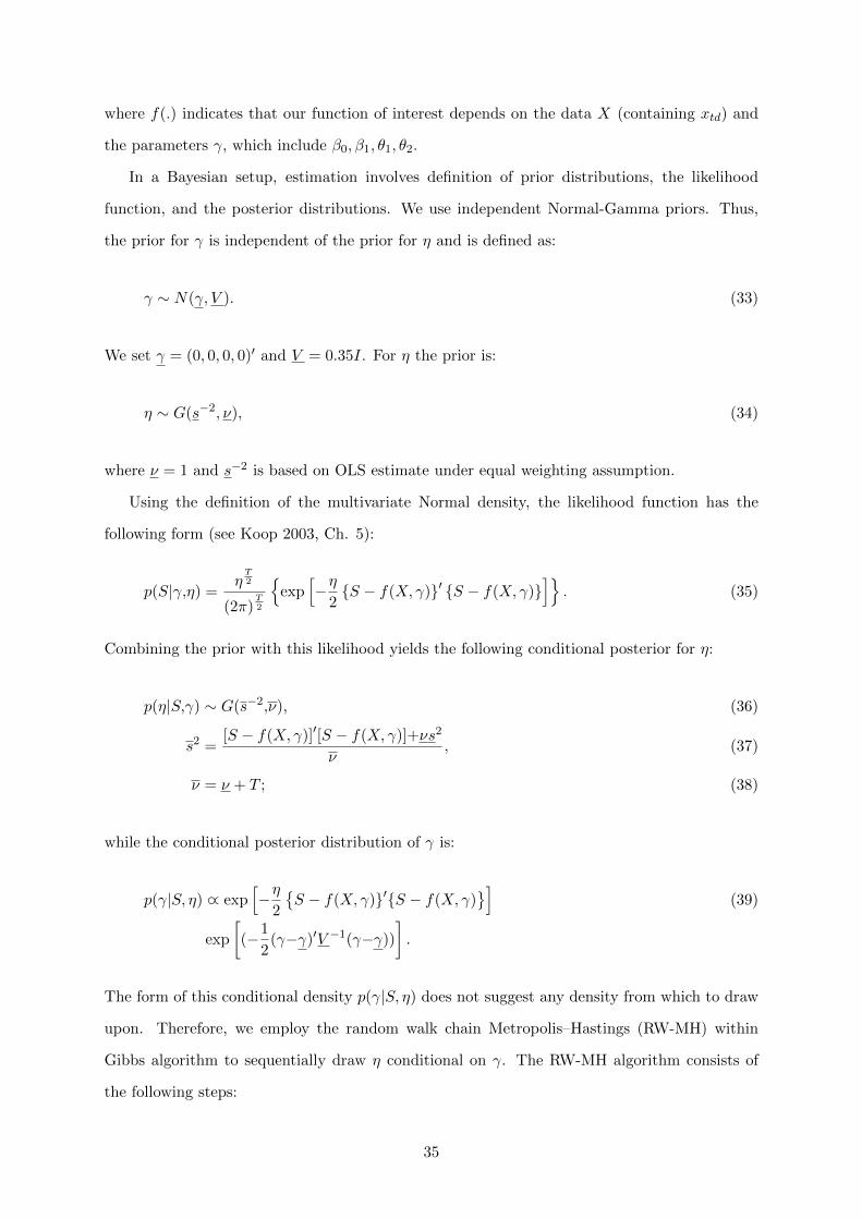
where f(.) indicates that our function of interest depends on the data X (containing xtd) and
the parameters γ, which include β0, β1, θ1, θ2.
In a Bayesian setup, estimation involves definition of prior distributions, the likelihood
function, and the posterior distributions. We use independent Normal-Gamma priors. Thus,
the prior for γ is independent of the prior for η and is defined as:
γ ∼ N(γ, V ). (33)
We set γ = (0, 0, 0, 0)′ and V = 0.35I. For η the prior is:
η ∼ G(s−2, ν), (34)
where ν = 1 and s−2 is based on OLS estimate under equal weighting assumption.
Using the definition of the multivariate Normal density, the likelihood function has the
following form (see Koop 2003, Ch. 5):
p(S|γ,η) =η
T2
(2π)T2
{exp
[−η
2{S − f(X, γ)}′ {S − f(X, γ)}
]}. (35)
Combining the prior with this likelihood yields the following conditional posterior for η:
p(η|S,γ) ∼ G(s−2,ν), (36)
s2 =[S − f(X, γ)]′[S − f(X, γ)]+νs2
ν, (37)
ν = ν + T ; (38)
while the conditional posterior distribution of γ is:
p(γ|S, η) ∝ exp[−η
2
{S − f(X, γ)}′{S − f(X, γ)
}](39)
exp
[(−1
2(γ−γ)′V −1(γ−γ))
].
The form of this conditional density p(γ|S, η) does not suggest any density from which to draw
upon. Therefore, we employ the random walk chain Metropolis–Hastings (RW-MH) within
Gibbs algorithm to sequentially draw η conditional on γ. The RW-MH algorithm consists of
the following steps:
35
1. Choose starting values for η and γ(0):
We use data available up to the beginning of our first forecast to fix these values. Precisely,
we set η = 1/s2, where s2 is based on OLS estimates assuming that θ1 = θ2 = 0. Using
the same data, we maximize the likelihood function in (35) and set γ(0) = γ̂ML; i.e., to
maximum likelihood estimates under θ1 = θ2 = 0;
2. Draw η from its conditional posterior as given by Expression (36);
3. Conditional on η take a candidate draw, γ(∗), from the candidate candidate generating
density:
γ(∗) ∼ N(γ(0),Σ),
where Σ = var(γ̂ML) is the covariance matrix of the maximum likelihood estimator ob-
tained in step 1;
4. Calculate acceptance probability:
α(γ(dr−1), γ(∗)) = min[
p(γ=γ(∗)|S)p(γ=γ(dr−1)|S) , 1
],
where p() is evaluated at the current, γ(∗), and previous, γ(dr−1), draw using (39);
5. Set γ(dr) = γ(∗) with probability α(γ(dr−1), γ(∗)) else γ(dr) = γ(dr−1);
6. Repeat above steps many times (e.g. 31000) and after discarding the first draws (e.g.
1000), keep every third draw. Point estimates of the parameters are obtained as average
of the retained draws.
A.3 Prediction
Prediction is based on the predictive density (Koop 2003, Ch. 5):
p(S∗|S, γ) = t(S∗|f(X∗, γ), s2IT , T ), where s2 = (S − f)′(S − f)/T.
Given MN models defined by the predictors included, we first assign (diffuse) prior proba-
bilities to each: Pr(Mi) = 1/MN . Based on the model’s realized likelihood we obtain posterior
probabilities:
Pr(Mi|Dt) =Pr(Dt|Mi) Pr(Mi)∑MN
j=1 Pr(Dt|Mj) Pr(Mj), (40)
where Pr(Dt|Mi) is the marginal likelihood of the ith model. We use the Gelfand and Dey
(1994) method for marginal likelihood calculation. The method requires careful selection of the
36

probability density function from which to simulate draws. We follow the usual practice and
use a multivariate Normal density truncated to the region Θ̂:
Θ̂ = {γ : (γ̂ − γ)′v̂ar(γ)−1
(γ̂ − γ) ≤ χ21−p(dof)} (41)
where χ21−p(dof) is the (1-p) percentile of the Chi-squared distribution with degrees of freedom
(dof) determined by the number of parameters in γ. Thus, our truncated multivariate Normal
density function is:
f(γ) =1
p(2π)12dof
∣∣∣v̂ar(γ)∣∣∣− 1
2exp
[−1
2(γ̂ − γ)′v̂ar(γ)
−1(γ̂ − γ)
]1(γ ∈ Θ̂) (42)
with 1() denoting the indicator function.
37
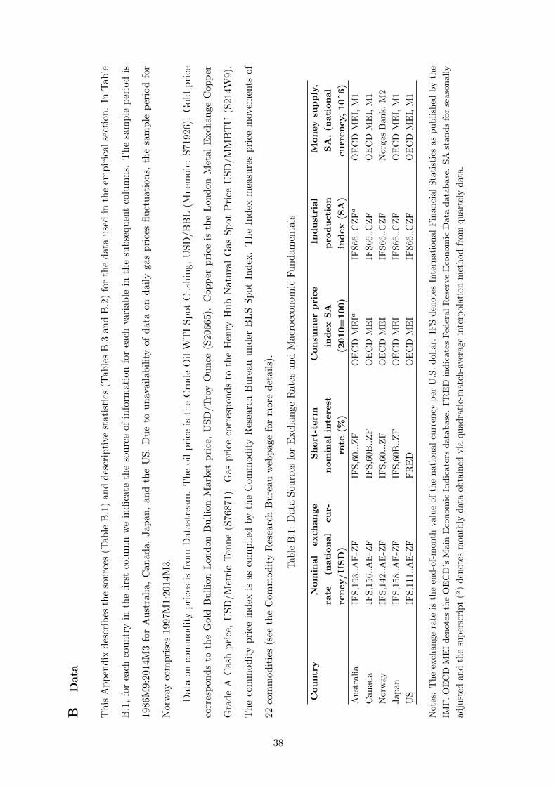
BData
Th
isA
pp
end
ixd
escr
ibes
the
sou
rces
(Tab
leB
.1)
and
des
crip
tive
stat
isti
cs(T
able
sB
.3an
dB
.2)
for
the
data
use
din
the
emp
iric
al
sect
ion
.In
Tab
le
B.1
,fo
rea
chco
untr
yin
the
firs
tco
lum
nw
ein
dic
ate
the
sou
rce
ofin
form
atio
nfo
rea
chva
riab
lein
the
sub
sequ
ent
colu
mn
s.T
he
sam
ple
per
iod
is
1986
M9:
2014
M3
for
Au
stra
lia,
Can
ada,
Jap
an,
and
the
US
.D
ue
tou
nav
aila
bil
ity
ofd
ata
on
dail
ygas
pri
ces
flu
ctu
ati
on
s,th
esa
mp
lep
erio
dfo
r
Nor
way
com
pri
ses
1997
M1:
2014
M3.
Dat
aon
com
mod
ity
pri
ces
isfr
omD
atas
trea
m.
Th
eoi
lp
rice
isth
eC
rud
eO
il-W
TI
Sp
otC
ush
ing,
US
D/B
BL
(Mn
emoic
:S
71926).
Gold
pri
ce
corr
esp
ond
sto
the
Gol
dB
ull
ion
Lon
don
Bu
llio
nM
arke
tp
rice
,U
SD
/Tro
yO
un
ce(S
2066
5).
Cop
per
pri
ceis
the
Lon
don
Met
al
Exch
an
ge
Cop
per
Gra
de
AC
ash
pri
ce,
US
D/M
etri
cT
onn
e(S
7687
1).
Gas
pri
ceco
rres
pon
ds
toth
eH
enry
Hu
bN
atu
ral
Gas
Sp
ot
Pri
ceU
SD
/M
MB
TU
(S214W
9).
Th
eco
mm
od
ity
pri
cein
dex
isas
com
pil
edby
the
Com
mod
ity
Res
earc
hB
ure
auu
nd
erB
LS
Sp
ot
Ind
ex.
Th
eIn
dex
mea
sure
sp
rice
mov
emen
tsof
22co
mm
od
itie
s(s
eeth
eC
omm
od
ity
Res
earc
hB
ure
auw
ebp
age
for
mor
ed
etai
ls).
Tab
leB
.1:
Dat
aS
ourc
esfo
rE
xch
ange
Rat
esan
dM
acro
econ
om
icF
un
dam
enta
ls
Country
Nominal
exch
ange
rate
(national
cur-
rency/USD)
Short-term
nominalintere
st
rate
(%)
Consu
merprice
indexSA
(2010=100)
Industrial
pro
duction
index(S
A)
Moneysu
pply,
SA,(n
ational
currency,10ˆ6)
Au
stra
lia
IFS
,193
..A
E-Z
FIF
S,6
0...
ZF
OE
CD
ME
IaIF
S66
..C
ZFa
OE
CD
ME
I,M
1
Can
ada
IFS,1
56.
.AE
-ZF
IFS
,60B
..Z
FO
EC
DM
EI
IFS
66..
CZ
FO
EC
DM
EI,
M1
Nor
way
IFS
,142
..A
E-Z
FIF
S,6
0...
ZF
OE
CD
ME
IIF
S66
..C
ZF
Nor
ges
Ban
k,
M2
Jap
anIF
S,1
58..
AE
-ZF
IFS
,60B
..Z
FO
EC
DM
EI
IFS
66..
CZ
FO
EC
DM
EI,
M1
US
IFS
,111
..A
E-Z
FF
RE
DO
EC
DM
EI
IFS
66..
CZ
FO
EC
DM
EI,
M1
Not
es:
Th
eex
chan
gera
teis
the
end
-of-
mon
thva
lue
ofth
en
atio
nal
curr
ency
per
U.S
.d
olla
r.IF
Sd
enot
esIn
tern
atio
nal
Fin
anci
alS
tati
stic
sas
pu
bli
shed
by
the
IMF
.O
EC
DM
EI
den
otes
the
OE
CD
’sM
ain
Eco
nom
icIn
dic
ator
sd
atab
ase.
FR
ED
ind
icat
esF
eder
alR
eser
ve
Eco
nom
icD
ata
dat
abas
e.S
Ast
and
sfo
rse
aso
nall
y
adju
sted
and
the
sup
ersc
rip
t(a
)d
enot
esm
onth
lyd
ata
obta
ined
via
qu
adra
tic-
mat
ch-a
ver
age
inte
rpol
atio
nm
eth
od
from
qu
arte
lyd
ata.
38
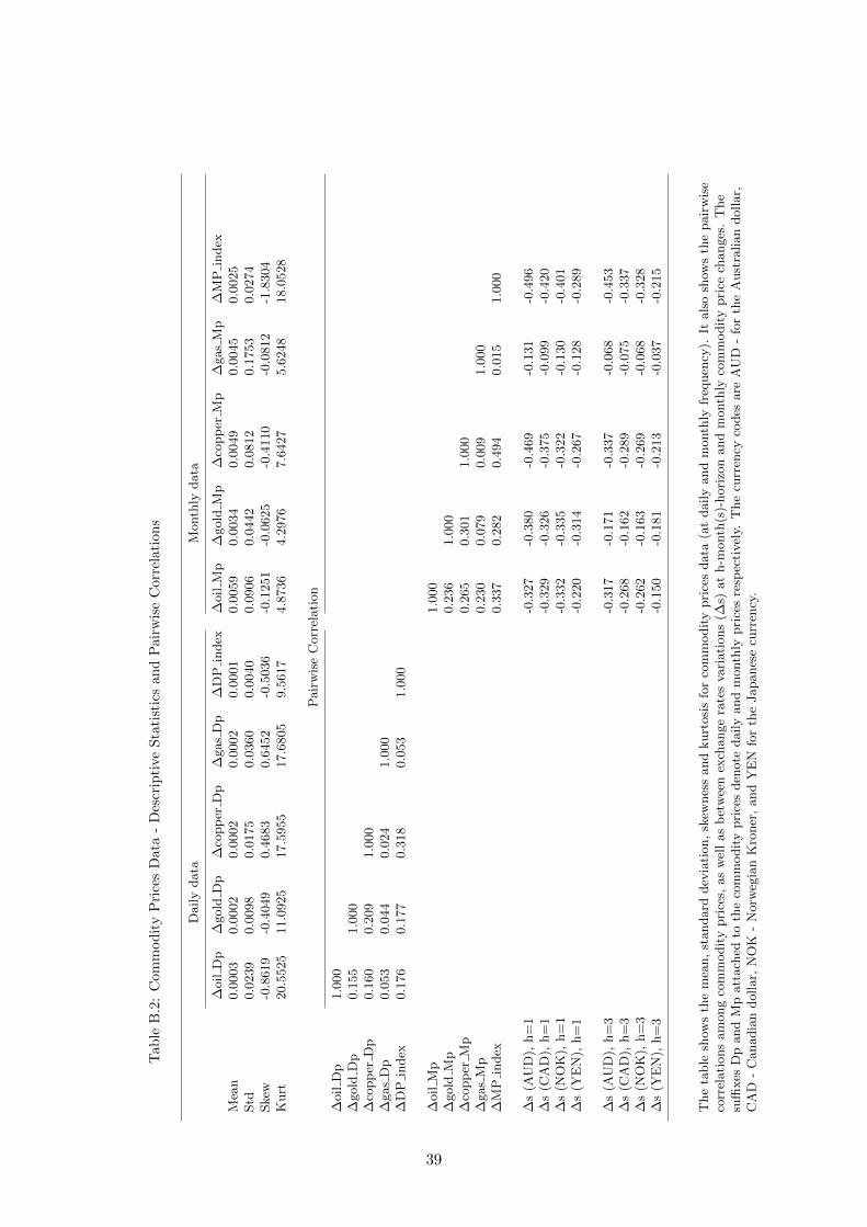
Tab
leB
.2:
Com
mod
ity
Pri
ces
Dat
a-
Des
crip
tive
Sta
tist
ics
and
Pai
rwis
eC
orre
lati
ons
Daily
data
Month
lydata
∆oil
Dp
∆gold
Dp
∆co
pp
erD
p∆
gas
Dp
∆D
Pin
dex
∆oil
Mp
∆gold
Mp
∆co
pp
erM
p∆
gas
Mp
∆M
Pin
dex
Mea
n0.0
003
0.0
002
0.0
002
0.0
002
0.0
001
0.0
059
0.0
034
0.0
049
0.0
045
0.0
025
Std
0.0
239
0.0
098
0.0
175
0.0
360
0.0
040
0.0
906
0.0
442
0.0
812
0.1
753
0.0
274
Skew
-0.8
619
-0.4
049
0.4
683
0.6
452
-0.5
036
-0.1
251
-0.0
625
-0.4
110
-0.0
812
-1.8
304
Kurt
20.5
525
11.0
925
17.5
955
17.6
805
9.5
617
4.8
736
4.2
976
7.6
427
5.6
248
18.0
528
Pair
wis
eC
orr
elati
on
∆oil
Dp
1.0
00
∆gold
Dp
0.1
55
1.0
00
∆co
pp
erD
p0.1
60
0.2
09
1.0
00
∆gas
Dp
0.0
53
0.0
44
0.0
24
1.0
00
∆D
Pin
dex
0.1
76
0.1
77
0.3
18
0.0
53
1.0
00
∆oil
Mp
1.0
00
∆gold
Mp
0.2
36
1.0
00
∆co
pp
erM
p0.2
65
0.3
01
1.0
00
∆gas
Mp
0.2
30
0.0
79
0.0
09
1.0
00
∆M
Pin
dex
0.3
37
0.2
82
0.4
94
0.0
15
1.0
00
∆s
(AU
D),
h=
1-0
.327
-0.3
80
-0.4
69
-0.1
31
-0.4
96
∆s
(CA
D),
h=
1-0
.329
-0.3
26
-0.3
75
-0.0
99
-0.4
20
∆s
(NO
K),
h=
1-0
.332
-0.3
35
-0.3
22
-0.1
30
-0.4
01
∆s
(YE
N),
h=
1-0
.220
-0.3
14
-0.2
67
-0.1
28
-0.2
89
∆s
(AU
D),
h=
3-0
.317
-0.1
71
-0.3
37
-0.0
68
-0.4
53
∆s
(CA
D),
h=
3-0
.268
-0.1
62
-0.2
89
-0.0
75
-0.3
37
∆s
(NO
K),
h=
3-0
.262
-0.1
63
-0.2
69
-0.0
68
-0.3
28
∆s
(YE
N),
h=
3-0
.150
-0.1
81
-0.2
13
-0.0
37
-0.2
15
The
table
show
sth
em
ean,
standard
dev
iati
on,
skew
nes
sand
kurt
osi
sfo
rco
mm
odit
ypri
ces
data
(at
daily
and
month
lyfr
equen
cy).
Itals
osh
ows
the
pair
wis
eco
rrel
ati
ons
am
ong
com
modit
ypri
ces,
as
wel
las
bet
wee
nex
change
rate
sva
riati
ons
(∆s)
at
h-m
onth
(s)-
hori
zon
and
month
lyco
mm
odit
ypri
cech
anges
.T
he
suffi
xes
Dp
and
Mp
att
ach
edto
the
com
modit
ypri
ces
den
ote
daily
and
month
lypri
ces
resp
ecti
vel
y.T
he
curr
ency
codes
are
AU
D-
for
the
Aust
ralian
dollar,
CA
D-
Canadia
ndollar,
NO
K-
Norw
egia
nK
roner
,and
YE
Nfo
rth
eJapanes
ecu
rren
cy.
39
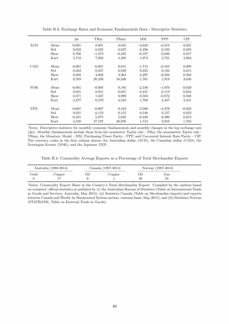
Table B.3: Exchange Rates and Economic Fundamentals Data - Descriptive Statistics
∆s TRsy TRasy MM PPP UIP
AUD Mean -0,001 0,001 0,033 -2,629 -0,319 0,031Std 0,032 0,035 0,037 0,498 0,192 0,025Skew 0,766 -1,373 -0,485 -0,197 0,036 0,917Kurt 5,718 7,092 4,385 1,974 2,731 3,983
CAD Mean -0,001 -0,001 0,015 -1,713 -0,165 0,008Std 0,022 0,037 0,039 0,335 0,133 0,015Skew 0,688 4,002 3,364 0,297 -0,350 0,568Kurt 9,359 20,236 16,326 1,761 1,919 3,638
NOK Mean -0,001 -0,005 0,185 -2,549 -1,870 0,029Std 0,031 0,031 0,031 0,447 0,119 0,024Skew 0,471 1,467 0,999 0,504 -0,872 0,848Kurt 4,277 6,579 4,583 1,780 3,447 3,431
YEN Mean -0,001 -0,007 0,442 0,586 -4,478 -0,023Std 0,031 0,153 0,155 0,548 0,137 0,023Skew -0,231 5,075 5,032 -0,340 0,390 0,012Kurt 4,556 27,197 26,950 1,513 3,010 1,704
Notes: Descriptive statistics for monthly economic fundamentals and monthly changes in the log exchange rate(∆s). Monthly fundamentals include those from the symmetric Taylor rule - TRsy, the asymmetric Taylor rule -TRasy, the Monetary Model - MM, Purchasing Power Parity - PPP, and Uncovered Interest Rate Parity - UIP.The currency codes in the first column denote the Australian dollar (AUD), the Canadian dollar (CAD), theNorwegian Kroner (NOK), and the Japanese YEN.
Table B.4: Commodity Average Exports as a Percentage of Total Merchandise Exports
Australia (1988-2014) Canada (1997-2014) Norway (1997-2014)
Gold Copper Oil Copper Oil Gas6 17 6 1 39 16
Notes: Commodity Export Share in the Country’s Total Merchandise Export. Compiled by the authors basedon countries’ official statistics as publised by (i) the Australian Bureau of Statistics (Table on International Tradein Goods and Services, Australia, May 2015); (ii) Statistics Canada (Table on Merchandise imports and exportsbetween Canada and World, by Harmonized System section, customs basis, May 2015); and (iii) Statistics Norway(STATBANK, Table on External Trade in Goods).
40
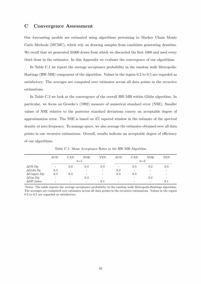
C Convergence Assessment
Our forecasting models are estimated using algorithms pertaining to Markov Chain Monte
Carlo Methods (MCMC), which rely on drawing samples from candidate generating densities.
We recall that we generated 31000 draws from which we discarded the first 1000 and used every
third draw in the estimates. In this Appendix we evaluate the convergence of our algorithms.
In Table C.1 we report the average acceptance probability in the random walk Metropolis-
Hastings (RW-MH) component of the algorithm. Values in the region 0.2 to 0.5 are regarded as
satisfactory. The averages are computed over estimates across all data points in the recursive
estimations.
In Table C.2 we look at the convergence of the overall RW-MH within Gibbs algorithm. In
particular, we focus on Geweke’s (1992) measure of numerical standard error (NSE). Smaller
values of NSE relative to the posterior standard deviations convey an acceptable degree of
approximation error. The NSE is based on 4% tapered window in the estimate of the spectral
density at zero frequency. To manage space, we also average the estimates obtained over all data
points in our recursive estimations. Overall, results indicate an acceptable degree of efficiency
of our algorithms.
Table C.1: Mean Acceptance Rates in the RW-MH Algorithm
AUD CAD NOK YEN AUD CAD NOK YENh=1 h=3
∆Oil Dp - 0.2 0.3 0.3 - 0.3 0.2 0.3∆Gold Dp 0.3 - - - 0.2 - - -∆Copper Dp 0.3 0.3 - - 0.3 0.3 - -∆Gas Dp - - 0.3 - - - 0.2 -∆DP index - - - 0.1 - - - 0.1
Notes: The table reports the average acceptance probability in the random walk Metropolis-Hastings algorithm.The averages are computed over estimates across all data points in the recursive estimations. Values in the region0.2 to 0.5 are regarded as satisfactory.
41
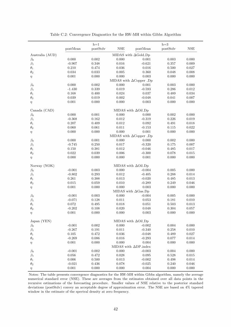
Table C.2: Convergence Diagnostics for the RW-MH within Gibbs Algorithm
h=1 h=3postMean postStdv NSE postMean postStdv NSE
Australia (AUD) MIDAS with ∆Gold Dpβ0 0.000 0.002 0.000 0.001 0.003 0.000β1 -0.907 0.348 0.016 -0.621 0.357 0.009θ1 0.210 0.474 0.036 0.016 0.500 0.027θ2 0.034 0.033 0.005 0.360 0.048 0.008η 0.001 0.000 0.000 0.003 0.000 0.000
MIDAS with ∆Copper Dpβ0 0.000 0.002 0.000 0.001 0.003 0.000β1 -1.430 0.339 0.019 -0.593 0.286 0.012θ1 0.168 0.400 0.024 0.037 0.489 0.034θ2 0.039 0.019 0.002 -0.048 0.041 0.007η 0.001 0.000 0.000 0.003 0.000 0.000
Canada (CAD) MIDAS with ∆Oil Dpβ0 0.000 0.001 0.000 0.000 0.002 0.000β1 -0.368 0.162 0.012 -0.319 0.226 0.019θ1 0.207 0.409 0.012 0.092 0.491 0.018θ2 0.060 0.061 0.011 -0.153 0.115 0.022η 0.000 0.000 0.000 0.001 0.000 0.000
MIDAS with ∆Copper Dpβ0 0.000 0.001 0.000 0.000 0.002 0.000β1 -0.745 0.250 0.017 -0.320 0.175 0.007θ1 0.150 0.381 0.012 -0.046 0.485 0.017θ2 0.022 0.039 0.006 -0.300 0.078 0.015η 0.000 0.000 0.000 0.001 0.000 0.000
Norway (NOK) MIDAS with ∆Oil Dpβ0 -0.001 0.003 0.000 -0.004 0.005 0.000β1 -0.802 0.293 0.012 -0.405 0.288 0.014θ1 0.261 0.388 0.013 -0.020 0.485 0.013θ2 0.015 0.059 0.010 -0.289 0.249 0.046η 0.001 0.000 0.000 0.003 0.000 0.000
MIDAS with ∆Gas Dpβ0 -0.001 0.003 0.000 -0.004 0.005 0.000β1 -0.071 0.128 0.011 0.053 0.181 0.010θ1 0.072 0.495 0.018 0.051 0.503 0.013θ2 -0.202 0.108 0.020 0.048 0.304 0.057η 0.001 0.000 0.000 0.003 0.000 0.000
Japan (YEN) MIDAS with ∆Oil Dpβ0 -0.001 0.002 0.000 -0.002 0.004 0.000β1 -0.267 0.191 0.011 -0.340 0.258 0.010θ1 0.105 0.472 0.036 -0.048 0.489 0.027θ2 -0.269 0.086 0.016 -0.293 0.077 0.014η 0.001 0.000 0.000 0.004 0.000 0.000
MIDAS with ∆DP indexβ0 -0.001 0.002 0.000 -0.003 0.004 0.000β1 0.056 0.472 0.028 0.095 0.528 0.015θ1 0.006 0.500 0.013 -0.002 0.498 0.014θ2 -0.021 0.436 0.078 -0.025 0.240 0.046η 0.001 0.000 0.000 0.004 0.000 0.000
Notes: The table presents convergence diagnostics for the RW-MH within Gibbs algorithm, namely the averagenumerical standard error (NSE). These are averages from the estimates obtained over all data points in therecursive estimations of the forecasting procedure. Smaller values of NSE relative to the posterior standarddeviations (postStdv) convey an acceptable degree of approximation error. The NSE are based on 4% taperedwindow in the estimate of the spectral density at zero frequency.
42
D Further Results Appendix
This Appendix reports further empirical results, including:
• Forecast assessment for single predictor models at 3-months horizon, in Table D.3;
• Forecast assessment for combination methods at 3-months horizon, in Table D.4.
The key findings are as follows. First, point forecasts based on daily commodity price
fluctuations are generally less precise than forecasts from the driftless Random Walk (RW) at
3-months forecasting horizon. This result is contrary to our findings at 1-month forecasting
horizon in the main text. Second, like our results at 1-month horizon, when we exploit density
forecasts we always find improvement over the RW at 3-months horizon. As shown in the right
panel of Table D.3, the log-score differentials are significantly positive in all cases. As well,
forecast combinations methods lead to more accurate forecasts than our benchmark.
43
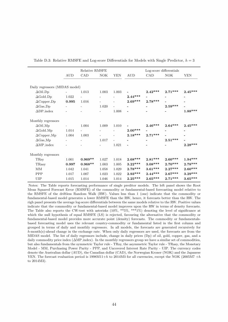
Table D.3: Relative RMSFE and Log-score Differentials for Models with Single Predictor, h = 3
Relative RMSFE Log-score differentials
AUD CAD NOK YEN AUD CAD NOK YEN
Daily regressors (MIDAS model)
∆Oil Dp - 1.013 1.003 1.003 - 2.42*** 2.71*** 2.45***
∆Gold Dp 1.022 - - - 2.44*** - - -
∆Copper Dp 0.995 1.016 - - 2.69*** 2.78*** - -
∆Gas Dp - - 1.020 - - - 2.59*** -
∆DP index - - - 1.008 - - - 1.88***
Monthly regressors
∆Oil Mp - 1.004 1.009 1.010 - 2.46*** 2.64*** 2.45***
∆Gold Mp 1.014 - - - 2.00*** - - -
∆Copper Mp 1.004 1.003 - - 2.18*** 2.71*** - -
∆Gas Mp - - 1.017 - - - 2.51*** -
∆MP index - - - 1.021 - - - 2.28***
Monthly regressors
TRsy 1.001 0.969** 1.027 1.018 2.68*** 2.81*** 2.60*** 1.94***
TRasy 0.997 0.968** 1.003 1.005 3.22*** 3.08*** 2.70*** 2.78***
MM 1.042 1.041 1.058 1.029 2.78*** 3.61*** 2.27*** 2.60***
PPP 1.017 1.007 1.023 1.022 2.93*** 2.44*** 2.67*** 3.29***
UIP 1.015 1.014 1.046 1.014 2.25*** 2.65*** 2.71*** 3.65***
Notes: The Table reports forecasting performance of single preditor models. The left panel shows the RootMean Squared Forecast Error (RMSFE) of the commodity or fundamental-based forecasting model relative tothe RMSFE of the driftless Random Walk (RW). Values less than 1 (one) indicate that the commodity orfundamental-based model generates a lower RMSFE than the RW, hence, it forecasts better than the RW. Therigh panel presents the average log-score differentials between the same models relative to the RW. Positive valuesindicate that the commodity or fundamental-based model improves upon the RW in terms of density forecasts.The Table also reports the CW-test with asterisks (10%, **5%, ***1%) denoting the level of significance atwhich the null hypothesis of equal RMSFE (LS) is rejected, favouring the alternative that the commodity orfundamental-based model provides more accurate point (density) forecasts. The commodity or fundamentals-based forecasting model uses the relevant country-commodity or fundamental listed in the first column andgrouped in terms of daily and monthly regressors. In all models, the forecasts are generated recursively forh-month(s)-ahead change in the exchange rate. When only daily regressors are used, the forecasts are from theMIDAS model. The list of daily regressors include, change in daily prices (Dp) of oil, gold, copper, gas, and adaily commodity price index (∆MP index). In the monthly regressors group we have a similar set of commodities,but also fundamentals from the symmetric Taylor rule - TRsy, the asymmetric Taylor rule - TRasy, the MonetaryModel - MM, Purchasing Power Parity - PPP, and Uncovered Interest Rate Parity - UIP. The currency codesdenote the Australian dollar (AUD), the Canadian dollar (CAD), the Norwegian Kroner (NOK) and the JapaneseYEN. The forecast evaluation period is 1998M11+h to 2014M3 for all currencies, except the NOK (2005M7 +hto 2014M3).
44

Table D.4: Relative RMSFE and CW-test for Forecast Combinations, h = 3
Daily regressors -Commodity Prices(CmdtyP)
Monthly regressors (Cmd-tyP and macro fundamen-tals)
Daily and monthly regres-sors (CmdtyP and macrofundamentals)
BMA BMS BMA BMS BMA BMS
AUD 0.998 0.996 0.999 0.998 0.997 0.997
CAD 0.995 0.995 0.975** 0.987** 0.975** 0.980**
NOK 1.007 1.001 1.025 1.013 1.021 1.006
YEN 0.996 0.994 1.014 1.018 1.012 1.016
OptPool EqWeights OptPool EqWeights OptPool EqWeights
AUD 0.998 1.004 1.026 1.009 1.024 1.008
CAD 0.991 0.996 0.980* 0.995 0.976** 0.998
NOK 1.005 1.008 1.042 1.022 1.040 1.019
YEN 0.999 1.001 1.041 1.004 1.047 1.003
Notes: The table reports the Root Mean Squared Forecast Error (RMSFE) for forecast combination methodsrelative to the RMSFE of the driftless Random Walk (RW). The methods include, Bayesian Model Averaging(BMA), Bayesian Model Selection, (BMS), the Optimal Predictive Pool (OptPool) of Geweke and Amisano(2011), and a simple equal-weighting scheme (EqWeights). Values less than 1 (one) indicate that the combinationmethod generates a lower RMSFE than the RW, hence, it forecasts better than the RW. The table also reportsthe CW-test with asterisks (10%, **5%, ***1%) denoting the level of significance at which the null hypothesisof equal RMSFE is rejected, favouring the alternative that the combination method has a lower RMSFE. Theforecast combinations are based on the relevant commodity-currency and standard macroeconomic fundamentals.For the Australian dollar (AUD) the relevant commodities are gold and copper; for the Canadian dollar (CAD)- oil and copper; and for the Norwegian Kroner (NOK) these include oil and gas. When only daily regressors areused the combination is based on forecasts from the MIDAS models - reported in columns [2-3]. In columns [4-5]the combination is based on forecasts from monthly regressors, while the last two columns report results fromcombining daily and monthly regressors. In all cases, the forecasts are generated recursively for h-month(s)-aheadchange in the exchange rate. In the group of monthly regressors we have a set of commodity pairs similar to thedaily group, but also fundamentals from the symmetric Taylor rule - TRsy, the asymmetric Taylor rule - TRasy,the Monetary Model - MM, Purchasing Power Parity - PPP, and Uncovered Interest Rate Parity - UIP. Theforecast evaluation period is 1998M11+h to 2014M3 for all currencies, except the NOK (2005M7 +h to 2014M3).
45
Recommended