Embed Size (px)
Citation preview
Forecasting Agricultural Commodity Transportation Costs:
Mississippi River Barge Rates
Brian Wetzstein, Zen-Noh Grain Corporation
Selected Paper prepared for presentation at the 2016 Agricultural & Applied Economics Association
Annual Meeting, Boston, Massachusetts, July 31-August 2
Copyright 2016 by [authors]. All rights reserved. Readers may make verbatim copies of this document for non-commercial purposes by any means, provided that this copyright notice appears on all such copies.
2
Forecasting Agricultural Commodity Transportation Costs:
Mississippi River Barge Rates
A commodities trader’s success is directly tied to his/her ability to foresee future changes in the
marketplace and to adapt a position accordingly. This is especially true in trading of agricultural
commodity markets that are characterized by low margins and high volumes. Intuition and
experience may provide a sense for the current feel of the market or even into the future;
however it is often difficult to convert feelings into numerical forecasts. Traders may then base
decisions on gut feelings or non-quantitative predictions based on intuition. A case in point is
commodity trading where transaction and transportation costs are generally a major variable-cost
component of the commodity being traded. These costs can represent a significant portion of
commodity-procurement costs, and in the case of Mississippi River barge shipping can be highly
volatile. Persistent changes in price volatility can heighten the risk exposure of both agricultural
producers and procurers, which negatively impacts efficiency by presenting a barrier to more
efficient trading and reduce the efficiency and competitiveness of U.S. exports. Organizations
augmenting their intuition with quantifiable predictions of commodity-procurement costs (barge
rates for example) may enhance their returns. Further, the Army Corps of Engineers as well as
state and federal governments are interested in barge rate forecasts as they are essentially
predictions of river traffic and commerce levels. These forecasts relate directly to the health of
the U.S. agricultural export market and domestic farmers.
When looking at how barge rates may behave in the future, many current traders rely simply
on a historical average or the barge rate in the previous period, which are naïve forecasting
scenarios that are unable to account for a changing market or external factors. An alternative is
3
developing an economic forecasting model to which improve the accuracy and reliability of
forecasts. Developing a simple model that yields more accurate forecasts than the current naïve
scenarios can increase trading profitability and transportation efficiency. However, the worth of
developing such a model extends farther than just improving trading efficiency and profitability.
It provides a case study on how applied economists are market engineers in designing tools for
improving efficiency. The real test of economic theory is not only how well it provides an
understanding of how an economy operates, but how well economists can apply the tools
developed from it to solve practical questions in a real world environment.
Thus, the aim of this analysis is to investigate the supply and demand dynamics of
agricultural commodity barge transportation and to produce simple spatial forecasts of barge
rates. These forecasts, along with increased understanding of variables affecting barge rates, can
lead to potential efficiency and monetary gains. The main goal is to predict barge rates and their
associated volatilities by river segment. The testable hypothesis is a simple spatial forecasting
model will out preform a naïve model in terms of yielding higher commodity trading returns
from taking advantage of more accurate barge rate forecasts.
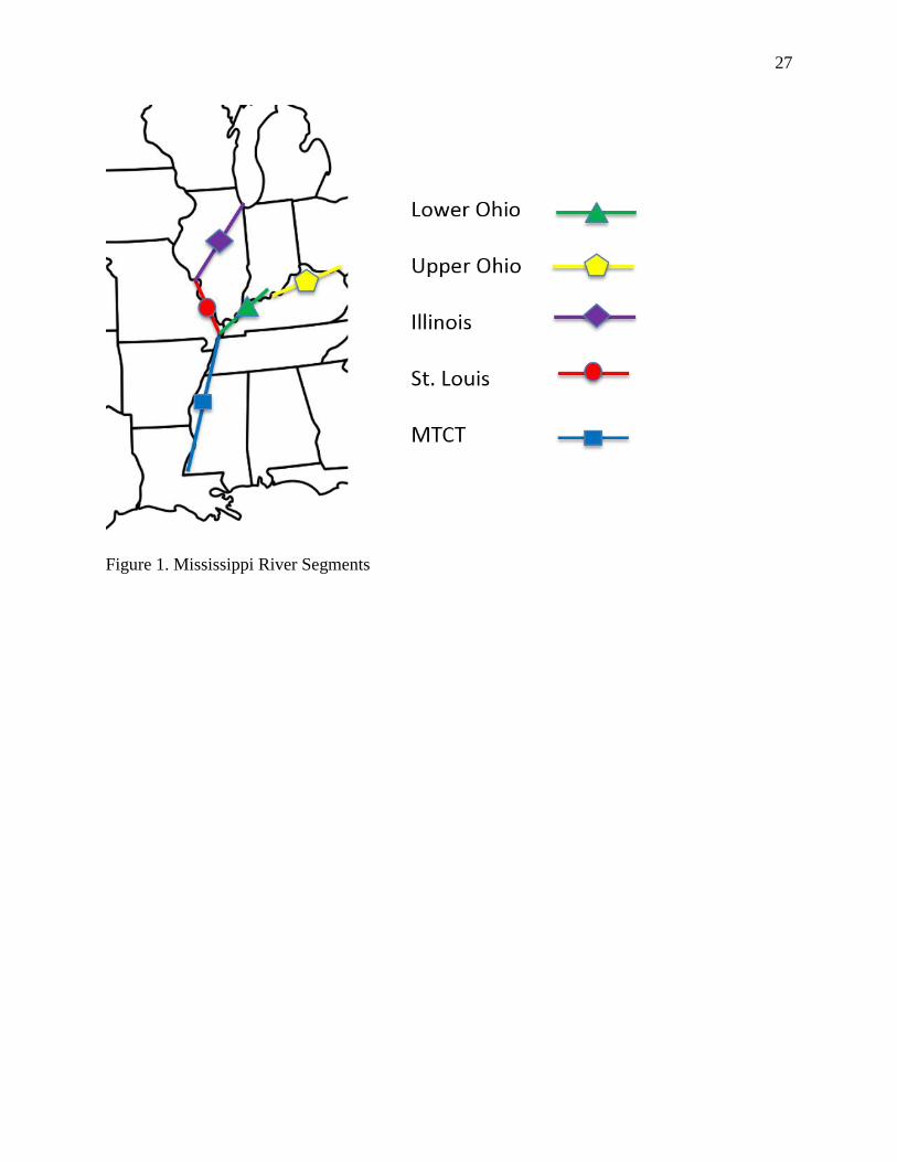
For forecasting barge rates by sector, a spatial vector autoregressive model is developed with
the dependent variables measuring the prices of barge transportation. Prices are in terms of five
distinct river segments: St. Louis, Illinois, Upper Ohio, Lower Ohio, and Lower Mississippi
(MTCT). The lagged spatial vector characteristics of the model capture segment price interaction
through time and space. In addition, exogenous variables of barge draft depth, Mississippi River
imports and exports, Midwest diesel prices, and first differenced corn prices are also included.
One-, two-, and five-week forecasts are constructed for an out-of-sample period. The
effectiveness and accuracy of the forecasts are then compared on the basis of RMSE, RMSPE,
4
stochastic dominance analysis, and the Henriksson-Merton test. Trader’s returns are then
conducted based on the resulting forecasts and the associated returns of conducting trades during
a period of low barge rates. Results support the hypothesis by indicating the forecasts have the
ability to improve on returns relative to a naïve forecasting scenario.
Literature
A wealth of literature exists on agricultural commodity pricing with the classic Tomek and
Robinson book as a foundation (Tomek and Robinson, 1972). Brandt and Bessler (1983) were
one of the first applications to apply time series analysis for forecasting agricultural commodity
prices. This was followed by efforts including Yang and Brorsen (1992) and Ramirez and
Fadiga (2003) who employ a GARCH model in forecasting. This research has resulted in regular
agricultural commodity price forecasts by various agencies including the World Bank (World
Bank, 2015).
In contrast, a review of the literature on forecasting within country U.S. agricultural
commodity transportation costs associated with barge transportation revealed no pertinent
articles. This is surprising given that transportation costs can represent a major proportion of
commodity costs (Schnepf, 2006; Volpe et al., 2013). A commodities trader considering future
purchases in the grain market for shipment to the Gulf of Mexico must forecast the cost of
transporting the grain from point-of-sale to the export port destination. Forecasting accuracy of
barge transportation rates directly impacts potential returns. There are some research efforts in
forecasting global rates of the large ocean going Panamax vessels. These include Batchelor et al.
(2007), Chang et al. (2012), and Chen et al. (2012) who employ VECM, ARIMA, and VARX
approaches, respectively, to forecast seaborne freight rates.
5
In terms of spatial econometrics, Kuethe and Pede (2011) indicate that estimating a
spatial VARX or SpVARX model for housing prices produced significantly more reliable short-
term forecasts than a conventional VARX model based on the mean-square forecast error. While
the variables affecting barge freight rate and housing prices are different, the underlying
methodology leading to a SpVARX model is still applicable. In a similar manner that nearby
housing prices can affect each other, barge rates in neighboring river segments do as well. The
inclusion of a spatial weight matrix to capture spillover effects in barge freight can aid in
improved model specification and the resulting forecasts.
Instead of developing improved methods or model specifications for predicting Mississippi
River barge rates, the literature improving the efficiency of river trade generally focuses on
infrastructure improvements to the lock and dam system. Current estimates from the Corps of
Engineers (2010) indicate it would cost approximately $3 billion dollars to renovate the aging
lock system to full working order. Yu et al. (2006) link lock delays to barge transportation
efficiency by employing a VAR model. Results suggest the strongest relation affecting barge
rates in different segments, apart from their own lagged values, are the lagged values of barge
rates in neighboring segments. If a segment’s barge rate can be reduced by increasing barge
supply, barge rates in neighboring segments will also decline. This suggests spatial
characteristics and interactions, which may be captured with a SpVARX model.
Barge Rates and Draft Depth
For analysis, the river is dissected into five distinct segments consisting of the Illinois, Upper
Ohio, Lower Ohio, Lower Mississippi (MTCT), and St. Louis rivers (Figure 1). This collection
of river segments comprises over 2000 miles of barge navigable waterways whose locks, dams,
6
and channels are maintained by the Army Corps of Engineers. The cost to ship commodities
between a specified river segment and a demand node to a Gulf port is given by lock tariff rates.
The Waterways Freight Bureau (WFB) was originally set up to regulate barge pricing. Each lock
had its own tariff rate measured as a dollar per ton cost to ship commodities between that lock
and a destination Gulf port. Since 1976, WFB no longer exists and market forces are allowed to
determine barge rates with 1976 tariffs as benchmarks.
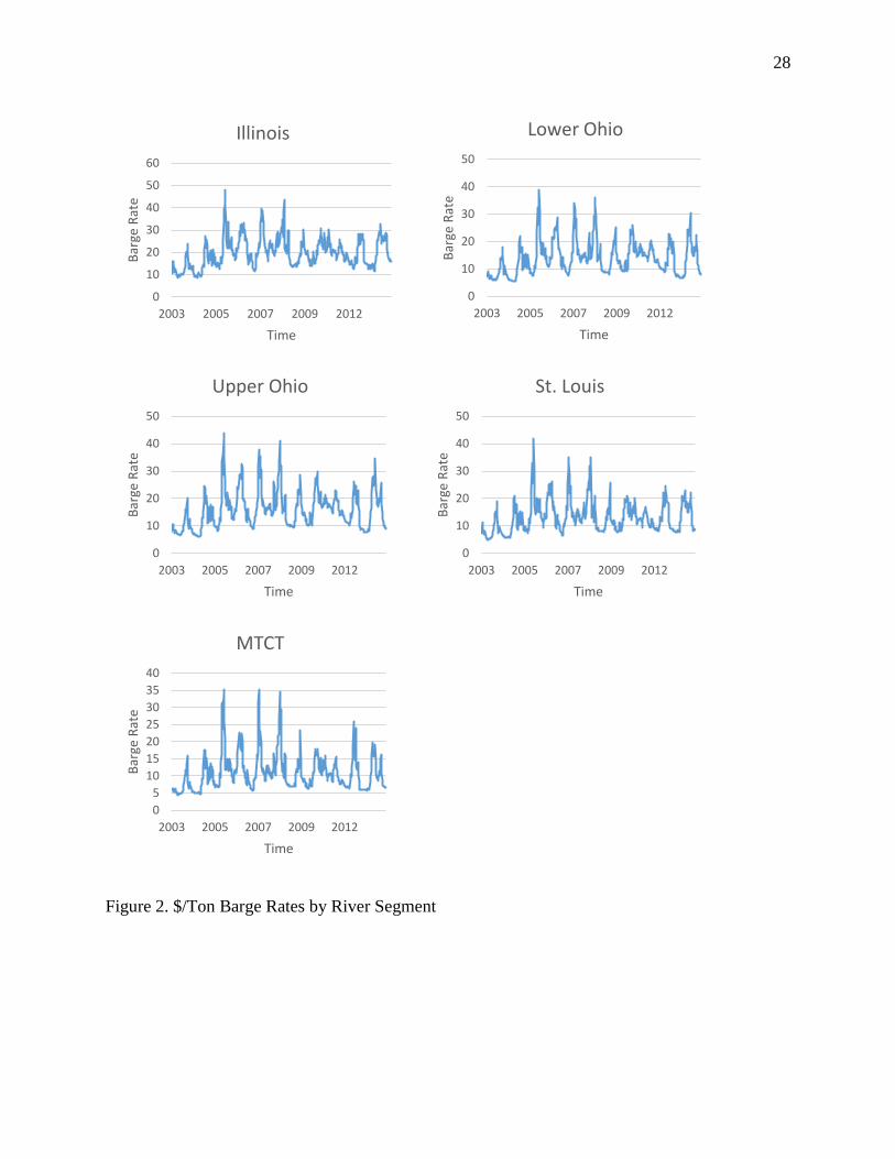
Barge operators on the Mississippi River employ a barge percent-of-tariff (BPOT) as the
price of traversing the river. Market forces then result in stochastic barge rates over time.
Multiplying the stochastic BPOT rate at a given time by the fixed historic tariff rate for a specific
lock within a given segment provides a dollar/ton price for shipping commodities. This price is
the cost per ton to ship a commodity from its starting location to a Gulf port. Overall, the rates
vary from approximately $2.00 to $7.00 per ton and are higher the farther north the lock location.
Figure 2 displays the barge rates in a dollar per ton value over the five river segments.
Market Structure
Miljkovic et al. (1999) concluded barge rates are determined by market forces with no
information asymmetries. Thus, the main elements to include in a forecasting model of barge
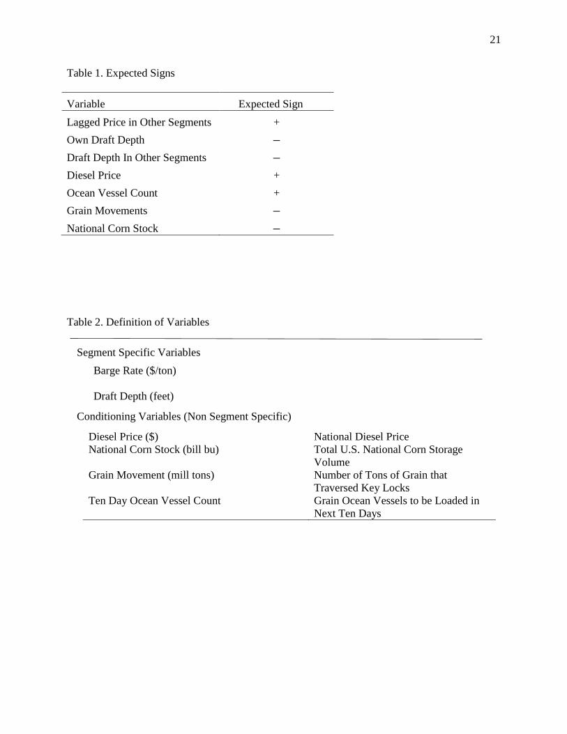
rates are variables influencing barge supply and demand. The list of the included variables along
with their expected signs are listed in Table 1.
One variable which influences the supply of barge transportation in the market is how
heavily barges can be loaded depending on current river conditions. The Army Corps of
Engineers attempt to maintain a minimum river channel depth of nine feet through dredging
policies, but are not always able to do so during drought or irregular river flow. However, most
7
of the volatility in loaded draft depth arises when natural river conditions permit barges to be
loaded deeper than nine feet. When river conditions are calm and sufficiently deep, barges can be
loaded to a maximum draft of around 12½’ to 13’. In these cases, theory would predict potential
lower barge rates as each barge can accommodate larger loads requiring fewer barges to be
contracted, and in essence increasing total barge transportation supply.
Another supply determinant is the availability of barges on a specific river segment. Grain
movements can serve as a proxy for segment supply availability. The U.S. Agricultural
Marketing Service tracks grain barge movements, which is similar to the barge count variable
employed by Yu et al. (2006). The main input price supply shifter is diesel prices where an
increase in fuel prices can negatively affect the availability of barges.
Covered dry cargo barge demand is primarily driven by the international transfer of grain
(Miljkovic et al., 1999), which is transported by ocean vessels. Over 90% of all U.S. corn and
soybean exports from the River Gulf area are transported there by barge. The number of
oceangoing grain vessels in the Gulf region can capture the quantity of covered cargo barge
transportation demand. The USDA Grain Inspection, Packers, and Stockyards Administration,
provides weekly measures of the number of oceangoing grain vessels scheduled for filling at the
Gulf Coast ports. Thus, larger numbers of vessels scheduled for filling at the gulf relate to
increased overall barge demand.
Available from the National Agricultural Statistics Service is the current level of U.S. corn
storage. With corn as main agricultural commodity transported by the barge type under study,
corn storage accounts for many of the seasonal characteristics of bar rates. When corn stocks are
trending down (up) this would suggest an increase (decrease) in barge demand.
8
The grain movements, national stock, and export variables focus on the downstream
movement of agricultural commodities. Variables specifically relating to the upstream
transportation of covered hopper barges are not included as there barge operate on a separate
price structure. Other than diesel prices, previous efforts addressing agricultural commodity
barge rates do not include specific variables to account for upstream transportation (Haigh and
Bryant, 2001; Fuller and Grant, 1993; Miljkovic et al., 1999). In addition with the majority of
upstream covered hopper barges empty, diesel prices capture a major portion of the upstream
transit cost. Further, once barges are loaded, it is rare the cargo does not travel the length of the
river as over 90% of agricultural commodity River Gulf exports are fed by barge. This
downstream dynamic is inherently included in the barge rate pricing system. The barge percent
of tariff barge rate of a specific lock is the cost of transportation between that specific lock
location and a downstream Gulf coast export location.
These downstream interactions yield a one directional relation where lower segments are
not affected by upper segments. This results in barge rate equation where a barge rate in a given
segment is a function of its own lagged price and the lagged price of segments below it. An
increase in barges rates in a segment downriver will stimulate up-bound barges to stop and
conduct business. This reduces the barge supply upriver. In contrast, if the barge rate were to
increase upriver, the supply of empty barges must still pass by the lower segments and will not
impact their barge supply.1 The interactions among segment draft depths are also a one
directional relation. Barge operators are only concerned with river levels downstream of their
loading site as this analysis deals with down bound barge rates.
9
Methodology
In econometrics, a spatial weight matrix is a tool used to identify possible spatial influences
within different portions of a system. It is often defined as a nonnegative matrix Wij, which
accounts for the spatial influence of unit j on unit i for n different spatial units (Bhattacharjee and
Jensen-Butler, 2013). In a distance based spatial weight matrix, neighboring segments are
assigned weights based on their relative distance. The weight is the inverse of their distance. For
barge freight, this distance is measured in river miles between the midpoints of respective
segments. A spatial weight matrix is then employed to examine how the percent of tariff barge
rate in one segment is related to current and past values of percent of tariff and draft depths in
neighboring segments. This is consistent with (Ollier et al., 2003), who employ a spatial weight
matrix to study the relation of segments sharing a common endpoint, as is the case with barge
rates in neighboring segments.
In order to include a weight matrix in the analysis and examine the effects of segment
interaction, s spatial cross-regressive lags are added to a VARX model (SpVARX). The
SpVARX(p,s) contains 𝑁 segments, which are specified as linear functions of 𝑝 own lags and 𝑝
lags of the other 𝑁 − 1 segments which are thought to influence it. Thus, which segments are
considered neighbors and how the neighbors are defined to effect each other are determined by
the structure of the weight matrix and the number of cross regressive lags. If a SpVARX(3,1) is
specified with s = 1, segments are considered neighbors only if they meet at a common point in
addition to the previously described one way interaction of only segments downstream affecting
ones upstream. This yields:
𝑌𝑛,𝑡 = 𝑐𝑛 + ∑ (𝛼𝑛,𝑝3𝑝=1 𝑌𝑛,𝑡−𝑝) + 𝛾𝑛𝑊𝑌𝑛,𝑡−1 + 𝛽𝑛𝑊𝐷𝑛,𝑡−1
10
+𝜎𝑛𝑋𝑛,𝑡−1 + 𝜀𝑛,𝑡, n = 1, …, 5,
where 𝑌𝑛,𝑡 is segment n barge rates observed in time 𝑡 = 1, … , 𝑇, 𝑊 is a spatial weight
matrix, 𝐷𝑛,𝑡−1 is a 5 × 1vector of draft depths by segment lagged one time period, 𝑋𝑛,𝑡−1 denotes
a 5 × 1vector of exogenous conditioning variables (draft depth, diesel price, ocean vessel count,
grain movements, and national corn stock) lagged one time period, 𝑐𝑛 is a constant term, 𝛼, 𝛽, 𝛾,
and 𝜎 are parameters to be estimated, and 𝜀𝑛,𝑡 is a white noise error term.
The spatial weight matrix, 𝑊, defines which segments are considered neighbors. The spatial
cross regressive lags are obtained by multiplying each temporal lag term by the spatial weight
matrix. These cross regressive lags represent the average barge rates of neighboring segments in
a previous time period. One commonly employed weighting system for spatial analysis is a
binary contiguity matrix where neighboring regions take a value of one with zero otherwise. A
second weighting scheme employed is an inverse distance based weight matrix. Each non-zero
element between two neighboring segments is assigned the value of 1/distance. Here, distance is
defined as the distance in river miles between the midpoints of each segment. The weight
matrixes are then row standardized to create proportional weights. Both weighting schemes yield
similar empirical results and forecasts, so only the weighting scheme analyses are presented
using row standardized weight matrices.
Data
For all the variables (barge rates, draft depths, diesel prices, corn storage, grain movements, and
ocean vessels) weekly data are collected from January 2003 to June 2014, yielding 594
11
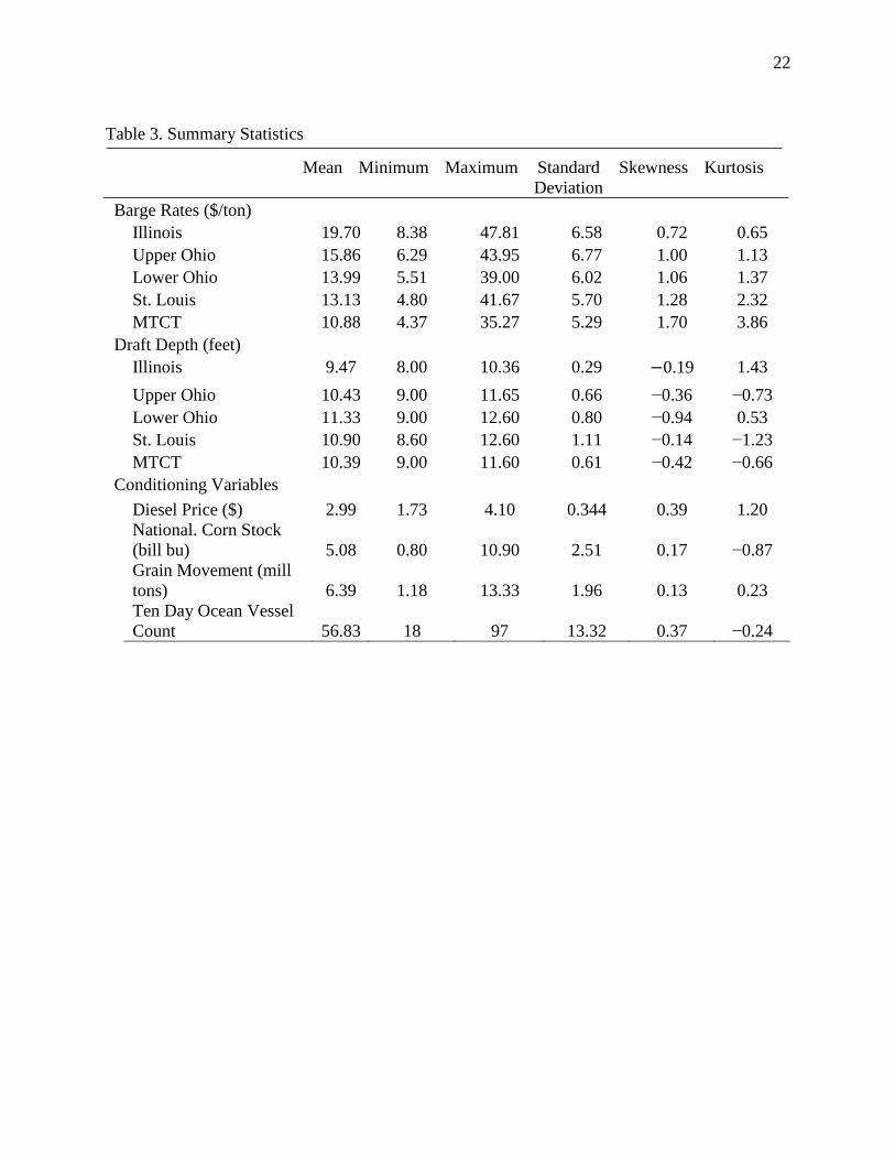
observations. The units of measurement and definitions are listed in Table 2 with summary
statistics provided in Table 3.
Barge rates have a relatively high variance with both a positive skewness and kurtosis. This
indicates river segment price distributions with right tails and frequent peaked high values. In
contrast, draft depths have left tail distributions with no consistency in the peaks. In terms of the
conditioning variables, ocean vessels have a relatively large standard deviation with close to a
normal distribution which is caused by the highly seasonal nature of agricultural commodity
exports. This is in contrast to diesel prices with relatively small standard deviations, but high
kurtosis.
Results
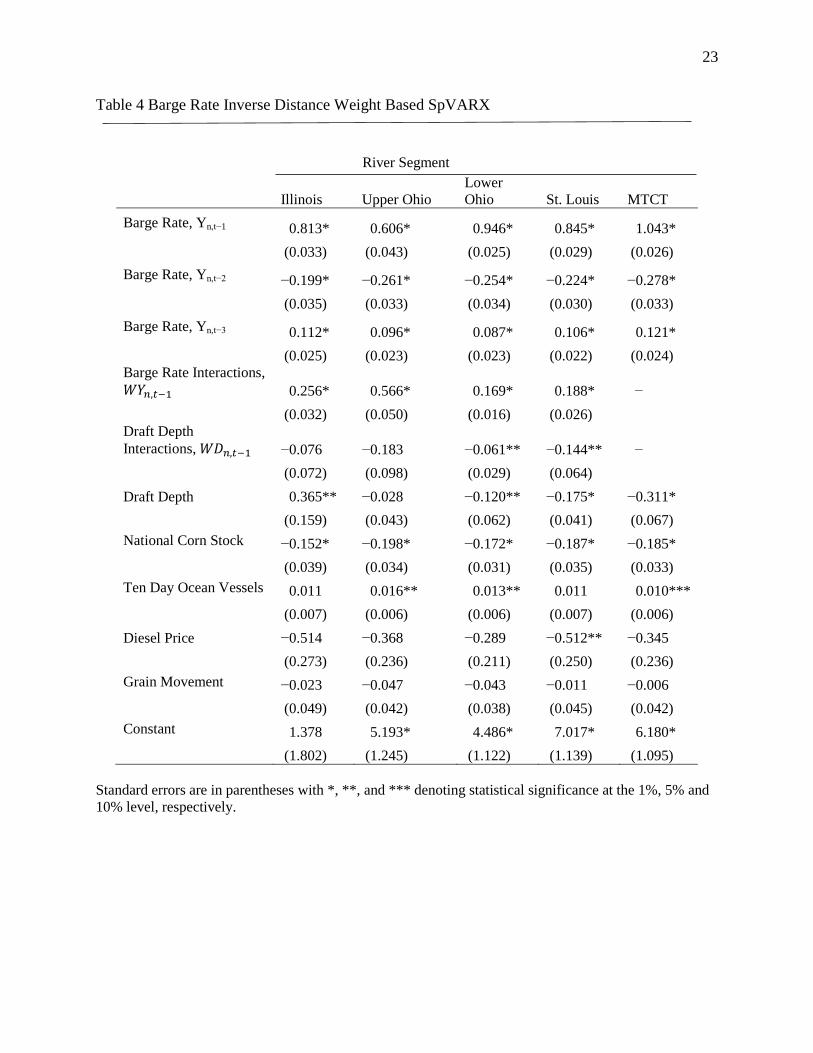
Table 4 lists the results of the SpVARX employing row standardized inverse distance weight
matrices.2 All of the self-lagged barge rates are significant at the 1% level with dynamics
indicating an adjustment process. The once lagged barge rates have a positive correlation with
current barge rates, followed by a negatively correlated second lag and positively correlated third
lag. The once lagged barge rates in neighboring segments representing price interaction terms are
also all significant at the 1% level. In terms of draft depth interaction terms, only the Lower Ohio
and St. Louis once lagged values of the draft depth interactions are significant. A segment’s own
lagged draft depth is significant with the hypothesized negative relation for the Lower Ohio, St.
Louis, and MTCT segments. A significant positive relationship at the 5% level between barge
rates and draft depth is associated with the Illinois segment and appears counter to the expected
coefficient sign. A hypothesis for this phenomenon is barges originating in the far northern
region of the Illinois are not constrained by draft depth. The average draft depth for this segment
12
is lower than the draft depth for the other segments (Table 3). Barge operators may load barges
originating in the Illinois segment only partially full with the idea that elevators farther south will
add cargo. Thus, a lower initial draft in Illinois could indicate decreased barge demand in the
Illinois segment compared to downriver segments and would reduce the barge rate in the Illinois
segment.
Each of the significant exogenous variables has the hypothesized sign with the exception of
diesel prices on the St. Louis segment. The lack of a significant diesel price relation for four of
the segments and a negative relation for the St. Louis segment indicates a weak adjustment
process of barge supply to input price changes. Barge rates appear slow to adjust to input price
changes. Input prices in general and diesel prices in particular appear to be less understood and
could be a point for further research and analysis.
Forecasting
In order to assess the predictive value of the model, One-, two-, and five-week forecasts are
constructed for an out-of-sample period. For out-of-sample forecasts, the last 20% of the 594
weekly observations are withheld in estimating the model. This yields an out-of-sample
forecasting range beginning in the seventh week of 2012 and continuing until the end of the full
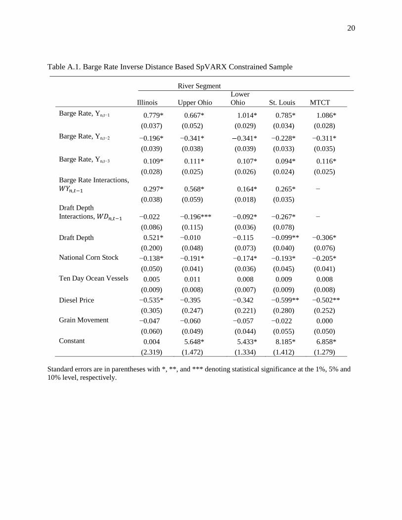
data set in week 23 of 2014. The Appendix Table A.1 lists estimation results, which are then
employed to estimate one-, two-, and five-week forecasts for the remaining 20% of the data.
Comparing the coefficients in Table 4 (the full sample) with Table A.1 (data-constrained sample)
reveals the stability of the results.
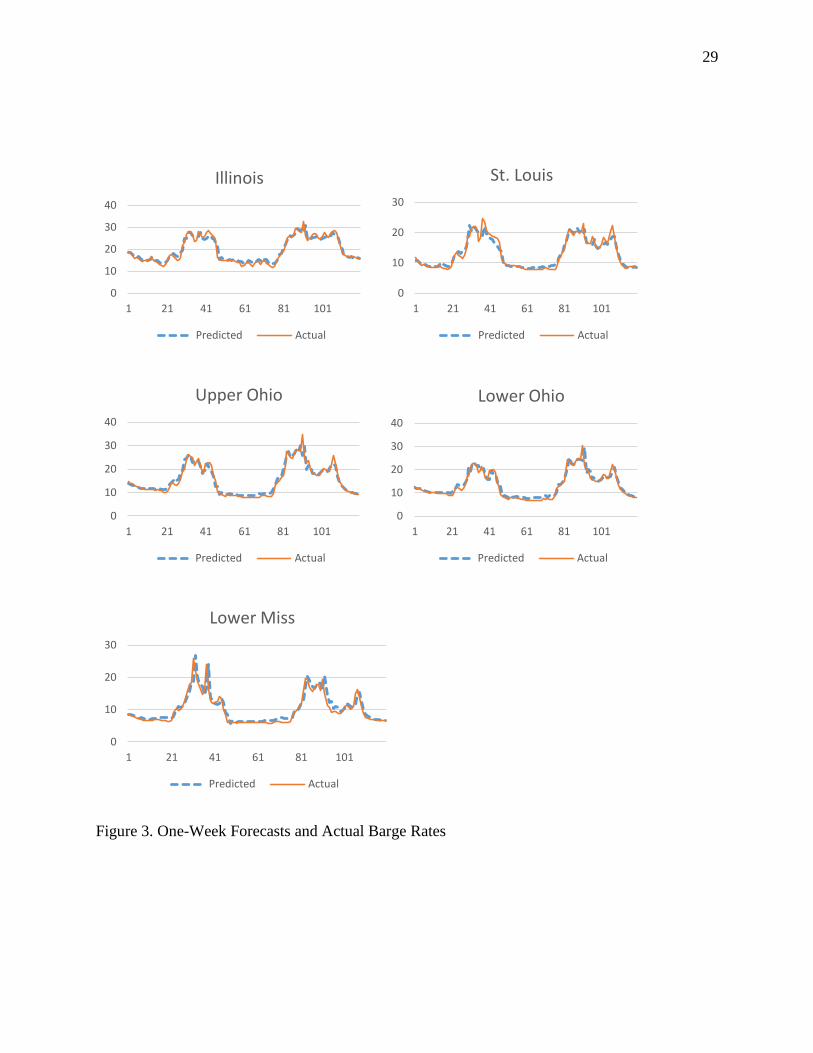
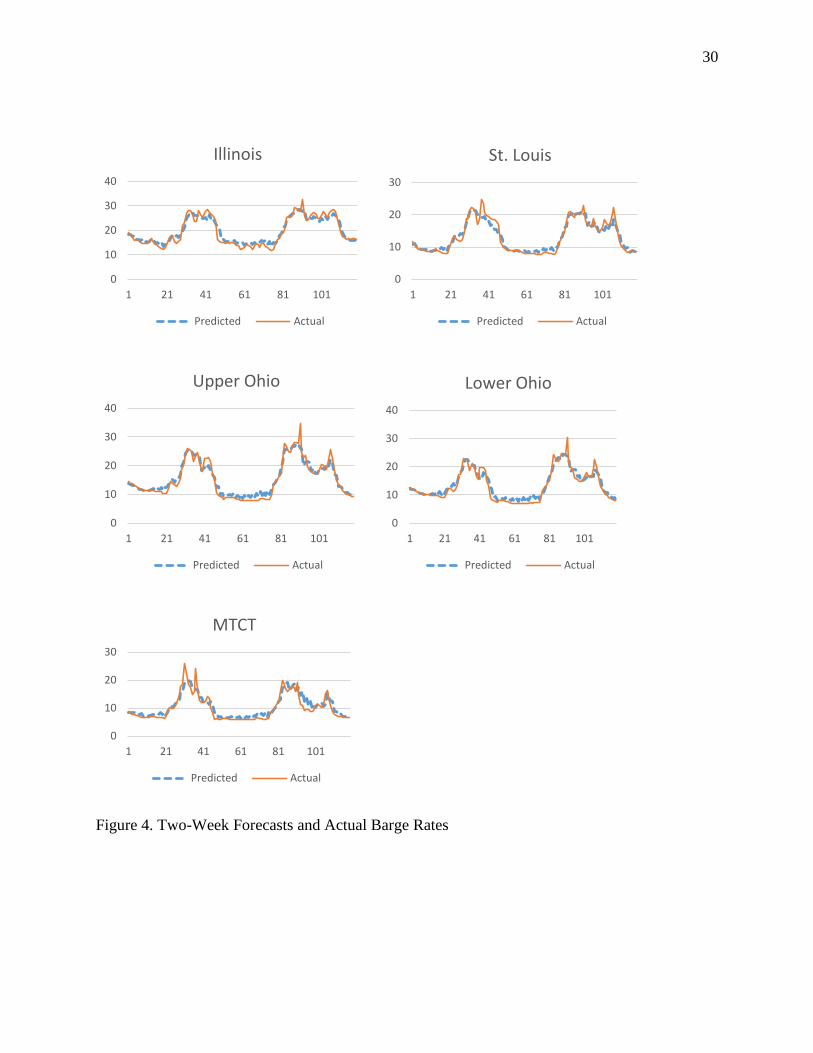
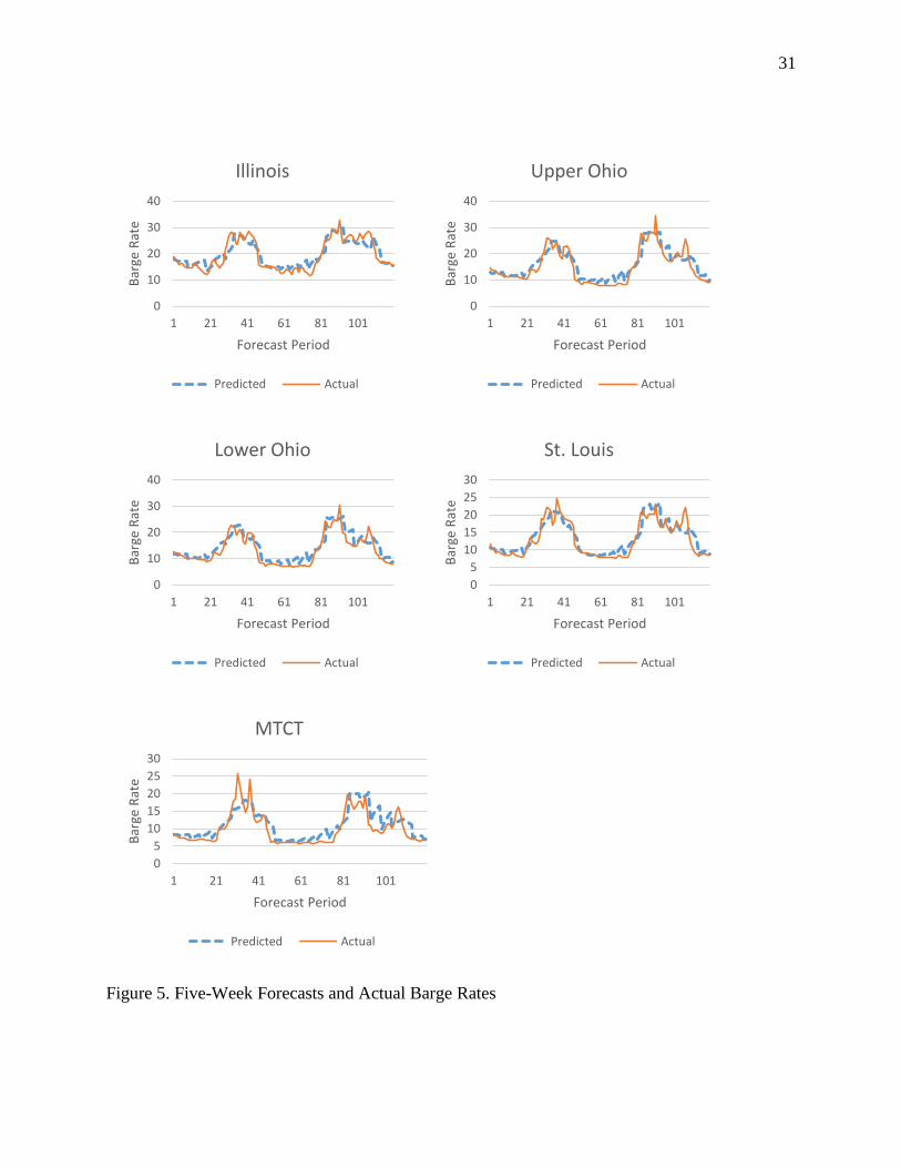
As a visual comparison, the predicted one-, two-, and five-week values are plotted against
their actual values for each river segment (Figures 3-5). The forecasts appear to track relatively
13
well for the one-week forecasts; deviations in their tracking exist as the forecasts are extended to
two and five weeks.
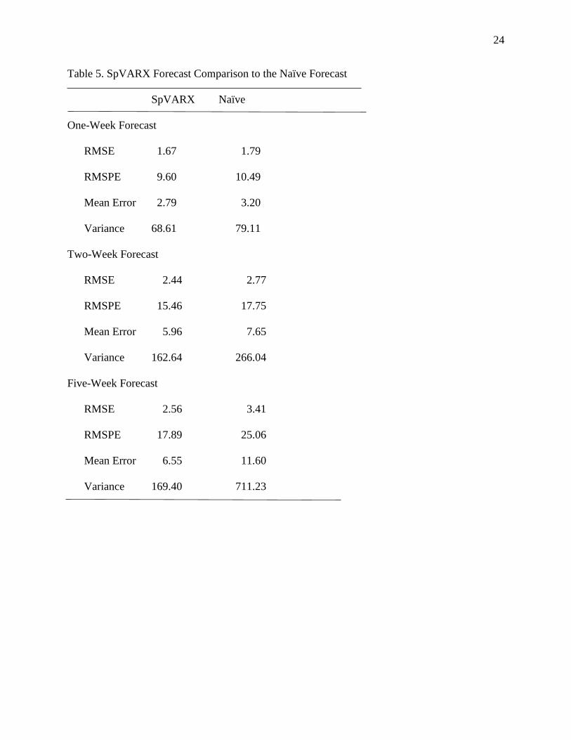
For numerical comparisons the root mean squared error (RMSE) and percent error (RMSPE)
are calculated along with the mean and variance for each forecast (Table 5). These values are
compared to a naïve forecasting model where the price in the next week is assumed to be the
price in the current week. Considering the one-week forecast, the naïve forecast is close to the
SpVARX forecast performance, although the SpVARX still dominates in terms of mean-
variance analysis. This close comparison does not continue to hold as the forecast length
increases. At the five-week forecast, the naïve forecasts deviate considerably from the actual
barge rates and the associated SpVARX forecasts. If there were only an interest in one-week
forecast, then the naïve forecasts would generally suffice. However, for any longer forecasting
period, a SpVARX type forecast is warranted.
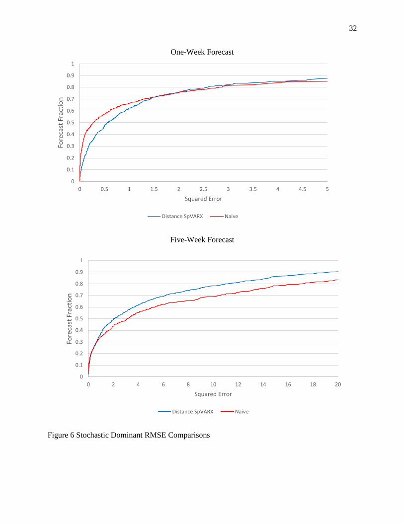
Considering stochastic dominance, a commodity trader’s gamble is choosing when to
purchase barge transportation based on assumption of how rates will change in the future. For
example, if barge rates are predicted to decline, a trader can gamble and delay commodity
transportation. Figure 6 illustrates the distribution of squared error terms for the one- and five-
week forecasts for a SpVARX model and the naïve forecasting case. All of the squared error
values for each forecast are sorted from low to high. With 120 out-of-sample forecasts and five
segments, there are 600 squared error terms for each forecast. The x-axis represents the squared
error terms y-axis is the accumulative probability from 1/600 to one. Thus, if a forecast’s
accumulative probability is farther to the left relative to another forecast’s, then it has a lower
squared error value for a higher percentage of its 600 observations. From Figure 6, the SpVARX
14
forecasts exhibit second-order stochastic dominance over the naïve forecasts. This supports their
numerical dominance presented in Table 5.
As a final comparison of the forecasts, the generalized Henriksson-Merton test is
employed as a market timing test to determine whether a forecast moves in the same
contemporaneous direction as the actual out-of-sample barge rates. Specifically, assuming no
preference symmetry on the part of traders, then
𝑟𝑓,𝑡+1 = 𝑐 + 𝛽𝑟𝑎,𝑡+1 + 𝜀𝑡+1,
where 𝑟𝑓,𝑡+1 and 𝑟𝑎,𝑡+1 denote the change in the forecast and actual barge rates from time t to t +
1, respectively, c and β are parameters to be estimated, and 𝜀𝑡+1 is the error term. The test
results reveal the β’s are positive and significant at the 1% level for the one-, two-, and five-
week forecasts. While the constants, c’s, are not significant. If there is no difference in the actual
and forecast barge rates values, the constant is zero. However, a trader with preference symmetry
would value these forecasts in terms of a positive significant relation between the first
differenced actual and forecasted values. When the actual barge rates increase (decrease) the
forecasted barge rates also increase (decrease) and there is not a significant constant, which
would imply a gap between their values.
Returns from Out-of-sample Forecasts
The results of the Henriksson-Merton test indicate the SpVARX forecasts have the ability to
improve commodity traders’ returns as the forecasted barge rates and actual barge rates tend to
move in the same direction. Traders could optimize their shipping schedule by correctly
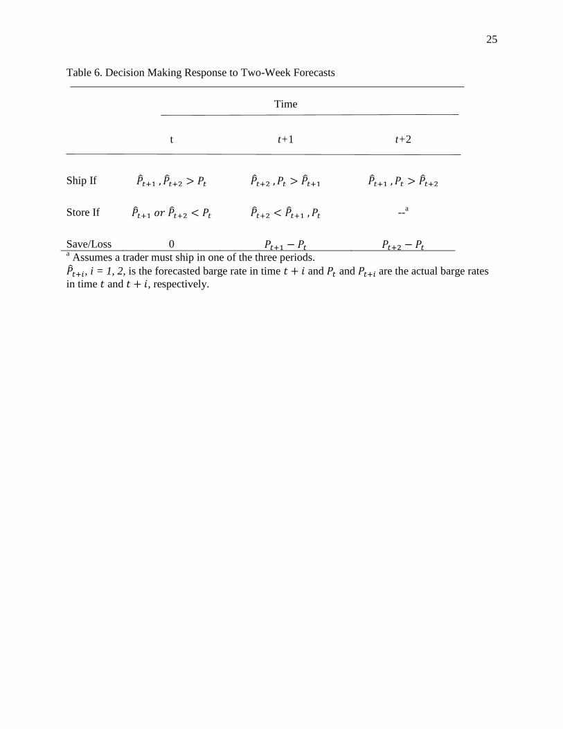
predicting the directional change of future barge rates. As an initial indication of the magnitude
of these potential enhanced returns, consider decision-making scenarios listed in Table 6 for a
15
two-week forecast. Let �̂�𝑡+𝑖, i = 1, 2, be the forecasted barge rate in time 𝑡 + 𝑖 and 𝑃𝑡 and
𝑃𝑡+𝑖 be the actual barge rates in time 𝑡 and 𝑡 + 𝑖, respectively. For simplicity, assume transaction
and storage costs are zero or constant. This allows focusing solely on transportation cost savings
when the trader is able to accurately take advantage of lower future barge rates. As indicated in
Table 6, this provides an examination of the potential savings or losses, which occur when a
trader uses the forecasted barge rates to take adjust their shipping schedule to take advantage of
lower rates.
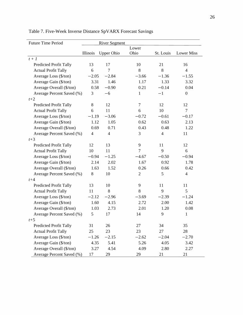
The decision-making process is extrapolated to the case of a five-week forecast. When
confronted with predicted barge rates for future periods, the lowest forecasted barge rate is
compared to the current barge rate. Thus, if a forecasted barge rate is lower than the current, in
this scenario the trader will chose to postpone shipment. The amount that the hypothetical trader
will ear/loss by adjusting their shipping schedule is the difference between the current barge rate
where they chose not to ship, and the actual observed barge rate when the forecasts implied
barge rates will be lower and when the trader in fact chose to ship. Table 7 lists the savings for a
five-week inverse distance based SpVARX forecast.
The predicted profit tally for each future time t + i, i = 1, …, 5 is the number of occurrences
that a forecasted barge rate in a set of 5 week forecasts is the lower than the current barge rate.
For t + 1, the predicted profit tally is the number of occurrences where �̂�𝑡+1 = min (�̂�𝑡+𝑖│𝑖 =
1, … ,5), and likewise for the other four future time periods. Commodity traders have a potential
to earn increased returns by transporting their goods during this forecasted lower barge rate
period. This predicted profit tally is mated to the actual profit tally where the actual barge rate
was indeed the lowest. For t+1, it is the number of occurrences where 𝑃𝑡+1 = min (𝑃𝑡+𝑖│𝑖 =
1, … ,5). When the forecast of the lowest future barge rate matches (does not match) the actual
16
week with the lowest rate, the trader experiences a savings (loss) in barge rates. The average
savings (loss) is then calculated based on the savings (loss) for each occurrence where �̂�𝑡+𝑖 −
𝑃𝑡+1 < 0 (�̂�𝑡+𝑖 − 𝑃𝑡+1 > 0). The overall average represents the average cost of barge
transportation that is saved or lost if these forecasts are followed. It represents the increase in
dollars per ton returns, which commodity traders would realize if they were to consistently adjust
their shipping schedule based on the SpVARX forecasts. Dividing this average overall savings
value by the average barge rate in the respective segment (Table 3) results in the average
percentage saved.
As indicated in Table 7, there is limited savings associated with the first future period, t + 1.
In fact, there is only a positive saving for the Illinois and Lower Ohio segments. Following the
naïve forecast would then be the recommended strategy. However, proceeding into the future
the average percentage saved with the SpVARX forecast generally increases. Consistent with
the forecast accuracy results (Table 5 and Figure 6), the SpVARX forecasts can potentially save
17% to 29% on barge rates when forecasts indicate optimal shipping is in the fifth week. If
commodity traders are interested in enhancing their returns associated with determining the
optimal shipping time, then they may want to consider some simple forecasting model, such as
the SpVARX.
Conclusions
The ability to accurately forecast Mississippi River barge rates provides trading advantages as
well as increasing market efficiency. This research outlines a forecasting model that can serve as
a foundation for agents, including traders, to develop quantifiable predictions of transportation
costs (barge rates). Such forecasts provide information to commodity traders when barge rates
17
are likely to be volatile. They can then minimize transportation costs by choosing to ship
commodities when rates are predicted to be lower. With these forecasts, traders are able to
optimize their shipping schedule by either transporting commodities now or storing them to ship
later.
As addressed in the introduction, a major avenue for economists is developing tools, which
solve practical questions of microeconomic engineering. One such tool is developing simple
forecasting models designed to augment existing future expectations. Specifically, the intricate
dynamics of agricultural commodity barge transportation on the Mississippi River is further
revealed through the engineering of simple barge-rate forecasts. With a five-week forecast
horizon, approximately 20% savings in barrage rates is possible when forecasts indicate lower
barge rates in five weeks. This supports the hypothesis that a simple spatial forecasting model
can out preform a naïve model. Economic engineering does have market value and suggests
agents may want to consider investing in such engineering. In particular, commodity traders can
benefit from these simple types of economic engineering.
18
Footnotes
1 Similar results are were obtained for a fully constrained and unconstrained model. The
downward bound model is presented as a representation.
2 Forecasting models were also developed based on VARX, directionally constrained VARX,
and binary SpVARX approaches. The inverse distance SpVARX model yields superior
forecasting performance, and thus, serves as the model for the reported results.
References
Batchelor, R., A. Alizadeh, I. Visvikis. 2007. “Forecasting Spot and Forward Prices in the
International Freight Market 23(1):101-114.
Bhattacharjee A, C. Jensen-Butler. 2013. “Estimation of the Spatial Weight Matrix under
Structural Constraints.” Regional Science and Urban Economics 43(4):617-634
Brandt, J., D. Bessler. 1983. “Price Forecasting and Evaluation: An Application in Agriculture,”
Journal of Forecasting 2(3):237-248.
Chang, C., C. Hsieh, Lin, Y. 2012. “A Predictive Model of the Freight Rate of the International
Market in Capesize Dry Bulk Carriers,” Applied Economics Letters 19(4):313-317.
Chen, S., H. Meersman, E. Van de Voorde. 2012. “Forecasting spot rates at main routes in the
dry bulk market,” Maritime Economics and Logistics 14(4):498-537.
Corps of Engineers. 2010. “Regional Supplement to the Corps of Engineers Wetland Delineation
Manual: Midwest Region (Version 2.0).” Wetlands Regulatory Assistance Program. U.S. Army
Corps of Engineers: Engineer Research and Development Center, August 2010.
http://www.usace.army.mil/Portals/2/docs/civilworks/regulatory/reg_supp/erdc-el-tr-10-16.pdf
Miljkovic D, G. Price, R. Hauser, K. Algozin. 1999. “The Barge and Rail Freight Market for
Export-Bound Grain Movement from Midwest to Mexican Gulf: An Econometric Analysis.”
Transportation Research Part E 36:127-137.
Ollier S, D. Chessel, P. Couteron, R. Pelissier, J. Thioulouse. 2003. “Comparing and Classifying
One-Dimensional Spatial Patterns: An Application to Laser Altimeter Profiles.” Remote Sensing
of Environment 4:453-462.
Ramírez, O., M. Fadiga. 2003. “Forecasting Agricultural Commodity Prices with Asymmetric-
Error GARCH Models,” Journal of Agricultural and Resource Economics 28(1):71-85.
Schnepf, R. 2006. Price Determination in Agricultural Commodity Markets: A Primer, CRS
Report for Congress, RL33204.
http://nationalaglawcenter.org/wp-content/uploads/assets/crs/RL33204.pdf
Tomek, W., K Robinson. 1972. Agricultural Product Prices, Ithaca: Cornell University Press.
19
Volpe, R., E. Roeger, E. Leibtag. 2013. How Transportation Costs Affect Fresh Fruit and
Vegetable Prices, ERR-160, Economic Research Service, USDA.
http://www.ers.usda.gov/media/1230835/err160.pdf
World Bank. 2015. Commodity Markets Outlook, A World Bank Quarterly Report, World Bank
Group.
https://www.worldbank.org/content/dam/Worldbank/GEP/GEP2015b/Global-Economic-
Prospects-CommodityMarketOutlook_Jan2015.pdf
Yang, S., B. Brorsen. 1992. “Nonlinear Dynamics of Daily Cash Prices,” American Journal of
Agricultural Econmics 74(3):706-715.
Yu, TH, D. Bessler, S. Fuller. (2006). “Effect of Lock Delay on grain Barge Rates: Examination
of Upper Mississippi and Illinois Rivers.” Ann. Reg. Sci. 40:887-908.
20
Table A.1. Barge Rate Inverse Distance Based SpVARX Constrained Sample
River Segment
Illinois Upper Ohio
Lower
Ohio St. Louis MTCT
Barge Rate, Yn,t−1 0.779* 0.667* 1.014* 0.785* 1.086*
(0.037) (0.052) (0.029) (0.034) (0.028)
Barge Rate, Yn,t−2 −0.196* −0.341* −0.341* −0.228* −0.311*
(0.039) (0.038) (0.039) (0.033) (0.035)
Barge Rate, Yn,t−3 0.109* 0.111* 0.107* 0.094* 0.116*
(0.028) (0.025) (0.026) (0.024) (0.025)
Barge Rate Interactions,
𝑊𝑌𝑛,𝑡−1 0.297* 0.568* 0.164* 0.265* −
(0.038) (0.059) (0.018) (0.035)
Draft Depth
Interactions, 𝑊𝐷𝑛,𝑡−1 −0.022 −0.196*** −0.092* −0.267* −
(0.086) (0.115) (0.036) (0.078)
Draft Depth 0.521* −0.010 −0.115 −0.099** −0.306*
(0.200) (0.048) (0.073) (0.040) (0.076)
National Corn Stock −0.138* −0.191* −0.174* −0.193* −0.205*
(0.050) (0.041) (0.036) (0.045) (0.041)
Ten Day Ocean Vessels 0.005 0.011 0.008 0.009 0.008
(0.009) (0.008) (0.007) (0.009) (0.008)
Diesel Price −0.535* −0.395 −0.342 −0.599** −0.502**
(0.305) (0.247) (0.221) (0.280) (0.252)
Grain Movement −0.047 −0.060 −0.057 −0.022 0.000
(0.060) (0.049) (0.044) (0.055) (0.050)
Constant 0.004 5.648* 5.433* 8.185* 6.858*
(2.319) (1.472) (1.334) (1.412) (1.279)
Standard errors are in parentheses with *, **, and *** denoting statistical significance at the 1%, 5% and
10% level, respectively.
21
Table 1. Expected Signs
Variable Expected Sign
Lagged Price in Other Segments +
Own Draft Depth −
Draft Depth In Other Segments −
Diesel Price +
Ocean Vessel Count +
Grain Movements −
National Corn Stock −
Table 2. Definition of Variables
Segment Specific Variables
Barge Rate ($/ton)
Draft Depth (feet)
Conditioning Variables (Non Segment Specific)
Diesel Price ($) National Diesel Price
National Corn Stock (bill bu) Total U.S. National Corn Storage
Volume
Grain Movement (mill tons)
Number of Tons of Grain that
Traversed Key Locks
Ten Day Ocean Vessel Count
Grain Ocean Vessels to be Loaded in
Next Ten Days
22
Table 3. Summary Statistics
Mean
Minimum
Maximum
Standard
Deviation
Skewness
Kurtosis
Barge Rates ($/ton)
Illinois 19.70 8.38 47.81 6.58 0.72 0.65
Upper Ohio 15.86 6.29 43.95 6.77 1.00 1.13
Lower Ohio 13.99 5.51 39.00 6.02 1.06 1.37
St. Louis 13.13 4.80 41.67 5.70 1.28 2.32
MTCT 10.88 4.37 35.27 5.29 1.70 3.86
Draft Depth (feet)
Illinois 9.47 8.00 10.36 0.29 −0.19 1.43
Upper Ohio 10.43 9.00 11.65 0.66 −0.36 −0.73
Lower Ohio 11.33 9.00 12.60 0.80 −0.94 0.53
St. Louis 10.90 8.60 12.60 1.11 −0.14 −1.23
MTCT 10.39 9.00 11.60 0.61 −0.42 −0.66
Conditioning Variables
Diesel Price ($) 2.99 1.73 4.10 0.344 0.39 1.20
National. Corn Stock
(bill bu) 5.08 0.80 10.90 2.51 0.17 −0.87
Grain Movement (mill
tons) 6.39 1.18 13.33 1.96 0.13 0.23
Ten Day Ocean Vessel
Count 56.83 18 97 13.32 0.37 −0.24
23
Table 4 Barge Rate Inverse Distance Weight Based SpVARX
River Segment
Illinois Upper Ohio
Lower
Ohio St. Louis MTCT
Barge Rate, Yn,t−1 0.813* 0.606* 0.946* 0.845* 1.043*
(0.033) (0.043) (0.025) (0.029) (0.026)
Barge Rate, Yn,t−2 −0.199* −0.261* −0.254* −0.224* −0.278*
(0.035) (0.033) (0.034) (0.030) (0.033)
Barge Rate, Yn,t−3 0.112* 0.096* 0.087* 0.106* 0.121*
(0.025) (0.023) (0.023) (0.022) (0.024)
Barge Rate Interactions,
𝑊𝑌𝑛,𝑡−1 0.256* 0.566* 0.169* 0.188* −
(0.032) (0.050) (0.016) (0.026)
Draft Depth
Interactions, 𝑊𝐷𝑛,𝑡−1 −0.076 −0.183 −0.061** −0.144** −
(0.072) (0.098) (0.029) (0.064)
Draft Depth 0.365** −0.028 −0.120** −0.175* −0.311*
(0.159) (0.043) (0.062) (0.041) (0.067)
National Corn Stock −0.152* −0.198* −0.172* −0.187* −0.185*
(0.039) (0.034) (0.031) (0.035) (0.033)
Ten Day Ocean Vessels 0.011 0.016** 0.013** 0.011 0.010***
(0.007) (0.006) (0.006) (0.007) (0.006)
Diesel Price −0.514 −0.368 −0.289 −0.512** −0.345
(0.273) (0.236) (0.211) (0.250) (0.236)
Grain Movement −0.023 −0.047 −0.043 −0.011 −0.006
(0.049) (0.042) (0.038) (0.045) (0.042)
Constant 1.378 5.193* 4.486* 7.017* 6.180*
(1.802) (1.245) (1.122) (1.139) (1.095)
Standard errors are in parentheses with *, **, and *** denoting statistical significance at the 1%, 5% and
10% level, respectively.
24
Table 5. SpVARX Forecast Comparison to the Naïve Forecast
SpVARX Naïve
One-Week Forecast
RMSE 1.67 1.79
RMSPE 9.60 10.49
Mean Error 2.79 3.20
Variance 68.61 79.11
Two-Week Forecast
RMSE 2.44 2.77
RMSPE 15.46 17.75
Mean Error 5.96 7.65
Variance 162.64 266.04
Five-Week Forecast
RMSE 2.56 3.41
RMSPE 17.89 25.06
Mean Error 6.55 11.60
Variance 169.40 711.23
25
Table 6. Decision Making Response to Two-Week Forecasts
Time
t t+1 t+2
Ship If �̂�𝑡+1 , �̂�𝑡+2 > 𝑃𝑡 �̂�𝑡+2 , 𝑃𝑡 > �̂�𝑡+1 �̂�𝑡+1 , 𝑃𝑡 > �̂�𝑡+2
Store If �̂�𝑡+1 𝑜𝑟 �̂�𝑡+2 < 𝑃𝑡 �̂�𝑡+2 < �̂�𝑡+1 , 𝑃𝑡 --a
Save/Loss 0 𝑃𝑡+1 − 𝑃𝑡 𝑃𝑡+2 − 𝑃𝑡 a Assumes a trader must ship in one of the three periods.
�̂�𝑡+𝑖, i = 1, 2, is the forecasted barge rate in time 𝑡 + 𝑖 and 𝑃𝑡 and 𝑃𝑡+𝑖 are the actual barge rates
in time 𝑡 and 𝑡 + 𝑖, respectively.
26
Table 7. Five-Week Inverse Distance SpVARX Forecast Savings
Future Time Period River Segment
Illinois Upper Ohio
Lower
Ohio St. Louis Lower Miss
t + 1
Predicted Profit Tally 13 17 10 21 16
Actual Profit Tally 6 7 8 8 4
Average Loss ($/ton) −2.05 −2.84 −3.66 −1.36 −1.55
Average Gain ($/ton) 3.31 1.46 1.17 1.33 3.32
Average Overall ($/ton) 0.58 −0.90 0.21 −0.14 0.04
Average Percent Saved (%) 3 −6 1 −1 0
t+2
Predicted Profit Tally 8 12 7 12 12
Actual Profit Tally 6 11 6 10 7
Average Loss ($/ton) −1.19 −3.06 −0.72 −0.61 −0.17
Average Gain ($/ton) 1.12 1.05 0.62 0.63 2.13
Average Overall ($/ton) 0.69 0.71 0.43 0.48 1.22
Average Percent Saved (%) 4 4 3 4 11
t+3
Predicted Profit Tally 12 13 9 11 12
Actual Profit Tally 10 11 7 9 6
Average Loss ($/ton) −0.94 −1.25 −4.67 −0.50 −0.94
Average Gain ($/ton) 2.14 2.02 1.67 0.92 1.78
Average Overall ($/ton) 1.63 1.52 0.26 0.66 0.42
Average Percent Saved (%) 8 10 2 5 4
t+4
Predicted Profit Tally 13 10 9 11 11
Actual Profit Tally 11 8 8 9 5
Average Loss ($/ton) −2.12 −2.96 −3.69 −2.39 −1.24
Average Gain ($/ton) 1.60 4.15 2.72 2.00 1.42
Average Overall ($/ton) 1.03 2.73 2.01 1.20 0.08
Average Percent Saved (%) 5 17 14 9 1
t+5
Predicted Profit Tally 31 26 27 34 35
Actual Profit Tally 25 23 23 27 28
Average Loss ($/ton) −1.26 −2.15 −2.62 −2.04 −2.70
Average Gain ($/ton) 4.35 5.41 5.26 4.05 3.42
Average Overall ($/ton) 3.27 4.54 4.09 2.80 2.27
Average Percent Saved (%) 17 29 29 21 21
27
Figure 1. Mississippi River Segments
28
Figure 2. $/Ton Barge Rates by River Segment
0
10
20
30
40
50
60
2003 2005 2007 2009 2012
Bar
ge R
ate
Time
Illinois
0
10
20
30
40
50
2003 2005 2007 2009 2012
Bar
ge R
ate
Time
Lower Ohio
0
10
20
30
40
50
2003 2005 2007 2009 2012
Bar
ge R
ate
Time
Upper Ohio
0
10
20
30
40
50
2003 2005 2007 2009 2012
Bar
ge R
ate
Time
St. Louis
0
5
10
15
20
25
30
35
40
2003 2005 2007 2009 2012
Bar
ge R
ate
Time
MTCT
29
Figure 3. One-Week Forecasts and Actual Barge Rates
0
10
20
30
40
1 21 41 61 81 101
Illinois
Predicted Actual
0
10
20
30
1 21 41 61 81 101
St. Louis
Predicted Actual
0
10
20
30
40
1 21 41 61 81 101
Upper Ohio
Predicted Actual
0
10
20
30
40
1 21 41 61 81 101
Lower Ohio
Predicted Actual
0
10
20
30
1 21 41 61 81 101
Lower Miss
Predicted Actual
30
Figure 4. Two-Week Forecasts and Actual Barge Rates
0
10
20
30
40
1 21 41 61 81 101
Illinois
Predicted Actual
0
10
20
30
1 21 41 61 81 101
St. Louis
Predicted Actual
0
10
20
30
40
1 21 41 61 81 101
Upper Ohio
Predicted Actual
0
10
20
30
40
1 21 41 61 81 101
Lower Ohio
Predicted Actual
0
10
20
30
1 21 41 61 81 101
MTCT
Predicted Actual
31
Figure 5. Five-Week Forecasts and Actual Barge Rates
0
10
20
30
40
1 21 41 61 81 101
Bar
ge R
ate
Forecast Period
Illinois
Predicted Actual
0
10
20
30
40
1 21 41 61 81 101
Bar
ge R
ate
Forecast Period
Upper Ohio
Predicted Actual
0
10
20
30
40
1 21 41 61 81 101
Bar
ge R
ate
Forecast Period
Lower Ohio
Predicted Actual
0
5
10
15
20
25
30
1 21 41 61 81 101
Bar
ge R
ate
Forecast Period
St. Louis
Predicted Actual
0
5
10
15
20
25
30
1 21 41 61 81 101
Bar
ge R
ate
Forecast Period
MTCT
Predicted Actual
32
One-Week Forecast
Five-Week Forecast
Figure 6 Stochastic Dominant RMSE Comparisons
0
0.1
0.2
0.3
0.4
0.5
0.6
0.7
0.8
0.9
1
0 0.5 1 1.5 2 2.5 3 3.5 4 4.5 5
Fore
cast
Fra
ctio
n
Squared Error
Distance SpVARX Naive
0
0.1
0.2
0.3
0.4
0.5
0.6
0.7
0.8
0.9
1
0 2 4 6 8 10 12 14 16 18 20
Fore
cast
Fra
ctio
n
Squared Error
Distance SpVARX Naive