Download pdf - Feasible estimation of firm-specific allocative inefficiency through Bayesian numerical methods

JOURNAL OF APPLIED ECONOMETRICSJ. Appl. Econ. 24: 675–697 (2009)Published online 2 April 2009 in Wiley InterScience(www.interscience.wiley.com) DOI: 10.1002/jae.1051

FEASIBLE ESTIMATION OF FIRM-SPECIFIC ALLOCATIVEINEFFICIENCY THROUGH BAYESIAN NUMERICAL

METHODS

SCOTT E. ATKINSONa AND JEFFREY H. DORFMANb*a Department of Economics, University of Georgia, Athens, GA, USA

b Department of Agricultural and Applied Economics, University of Georgia, Athens, GA, USA

SUMMARYBoth the theoretical and empirical literature on the estimation of allocative and technical inefficiency hasgrown enormously. To minimize aggregation bias, ideally one should estimate firm and input-specificparameters describing allocative inefficiency. However, identifying these parameters has often provendifficult. For a panel of Chilean hydroelectric power plants, we obtain a full set of such parameters usingGibbs sampling, which draws sequentially from conditional generalized method of moments (GMM) estimatesobtained via instrumental variables estimation. We find an economically significant range of firm-specificefficiency estimates with differing degrees of precision. The standard GMM approach estimates virtually noallocative inefficiency for industry-wide parameters. Copyright 2009 John Wiley & Sons, Ltd.

1. INTRODUCTION

The literature on efficiency measurement has been concerned with measuring economic efficiencyin terms of technical and allocative efficiency. Technical efficiency measures the actual inputusage relative to the minimum input usage for a given set of outputs or the actual outputs relativeto the maximum potential outputs for a given set of inputs. The technical efficiency of a firm ismeasured relative to the most efficient firm, which defines the production, distance, or cost frontier.Allocative efficiency measures how well firms manage the ratios of inputs in order to minimizethe cost of producing a given output. From the first-order conditions for cost minimization, firmsmust equate the ratio of marginal products to the ratio of input prices.

Allocative and technical efficiency have been measured using either an error-componentsapproach or a fixed-effects approach. With the latter approach, one estimates parameters thatmeasure allocative efficiency in a shadow distance system context by scaling input quantitiesor in a shadow cost system context by scaling input prices, yielding shadow input quantitiesand shadow input prices, respectively. Details are provided in Atkinson and Primont (2002).With the error-components approach, maximum likelihood techniques are typically used toestimate the parameters that define the distribution of a two-component error term, where a two-sided error represents noise and a one-sided error represents inefficiency specific to the firmor individual. Firm-specific measures of allocative and technical inefficiency are then obtainedfrom these estimated components. For a survey of this approach see Greene (1997). One major

Ł Correspondence to: Jeffrey H. Dorfman, Department of Agricultural and Applied Economics, University of Georgia,Athens, GA 30602, USA. E-mail: [email protected]

Copyright 2009 John Wiley & Sons, Ltd.

676 S. E. ATKINSON AND J. H. DORFMAN

drawback to this technique is that incorrect distributional assumptions on the error componentswill produce inconsistent estimators. A second shortcoming is that, owing to the complexitiesof using instruments in this setting, researchers typically make the often implausible assumptionthat the error terms are uncorrelated with the regressors, which must hold in order to avoidendogeneity. One error-components modeling approach has made the one-sided component afunction of explanatory variables.1 If this approach is taken, either these variables must beuncorrelated with the explanatory variables of the model itself to avoid omitted variable bias orappropriate instruments must be employed. Further, results may be very sensitive to the assumedfunctional form. If the distribution of the composed error is misspecified or if endogeneity isignored, parameter estimators will be inconsistent.

The fixed-effects approach avoids the need to specify the distribution of the errors or assume theexogeneity of the regressors. This approach easily allows testing for endogeneity and correctingfor its presence using instruments. Further, using this approach we can easily obtain robustestimated standard errors. The simplest fixed-effects approach would be to estimate time-invariant,input-specific allocative efficiency parameters. One can still estimate the effect on input over- orunder-utilization at the firm level by computing ratios of fitted input quantities. However, theassumption that all firms share common time-invariant allocative efficiency parameters for eachinput is a priori implausible. Estimation of time-varying, firm-specific (or plant-specific if data areavailable at this level) allocative efficiency parameters is generally preferred in order to reduceaggregation bias.

Estimation of a full set of firm-specific, time-varying allocative efficiency parameters has neverbeen previously accomplished. Rarely, in fact, have researchers been able to estimate a full setof firm-specific, time-invariant allocative efficiency parameters. Even with panel data and modelsthat are highly nonlinear in the parameters, which should assist identification, the data do nottypically contain enough independent variation to identify the full set of parameters measuringallocative efficiency along with the structural parameters that define stochastic cost, revenue,profit, distance, or production frontiers (the standard dual frontier paradigms). A random-effectsBayesian approach has been taken by Kumbhakar and Tsionas (2005), who estimate a translog costsystem using Gibbs sampling methods. However, their approach is subject to all the limitationsof the classical random-effects estimation approach and requires a full parametric specification ofthe structural model and the likelihood function. Further, they obtain firm-specific measures ofallocative efficiency which are not time-varying.

In this paper, we present a solution to this problem by substituting a semi-parametric Bayesianapproach implemented using a Markov chain Monte Carlo (MCMC) technique. Our MCMCapproach follows and extends Zellner and Tobias (2001), Kim (2002), and Atkinson and Dorfman(2005) by employing a limited information likelihood function that minimizes the assumptionsrequired for estimation, making it essentially equivalent to Bayesian generalized method ofmoments (GMM) with instruments. While we are fully parametric in the specification of thestructural model, we are non-parametric in the specification of the error distribution. A parallelsemi-parametric approach taken by Griffin and Steel (2004), Koop and Tobias (2006), and Koopand Poirier (2004) reverses the choice of the parametric and non-parametric components. Theyemploy a parametric likelihood function with a partially or fully non-parametric structural model.

For a panel of 12 Chilean hydroelectric power plants, we jointly estimate a translog input distancefunction and the first-order conditions from the dual shadow-cost minimization model. We obtain

1 See Huang and Liu (1994).

Copyright 2009 John Wiley & Sons, Ltd. J. Appl. Econ. 24: 675–697 (2009)DOI: 10.1002/jae

FEASIBLE ESTIMATION OF FIRM-SPECIFIC ALLOCATIVE INEFFICIENCY 677

the posterior densities for plant-specific and time-varying estimates of allocative efficiency, whilecorrecting for any endogeneity of the regressors. We are able to identify and precisely estimate thisrich parameterization, when we could not using the classical approach, because we iteratively drawfrom a series of conditional posterior densities for the parameters using MCMC. Time-varying andplant-specific measures of technical efficiency (TE) are computed residually along with estimatesof productivity change (PC), which can be decomposed into technical change (TC) and efficiencychange (EC).

Our empirical findings are that energy is under-utilized in five plants (due to limited wateravailability or restrictions on water release) by as much as 18% and over-utilized in the rest byas much as 18%. Labor is over-utilized in seven plants by as much as 27% and under-utilizedin six plants by as much as 14%. Average rates across all plants are considerably smaller. Littlemovement toward allocative efficiency is observed over time for any plant. Technical efficiencyis low for many plants and productivity change and efficiency change vary widely across plants.For example, PC ranges from 2% to 12% across plants for year 9 of the sample. Finally, were-estimated our model using industry-wide allocative inefficiency parameters in place of plant-specific ones. The aggregate allocative inefficiency parameters indicate no appreciable allocativeinefficiency overall and mask important differences among the plant-specific parametric estimateswith regard to central tendency as well as precision.

2. FIRM-SPECIFIC ALLOCATIVE AND TECHNICAL INEFFICIENCY

To model firm-specific allocative inefficiency we follow Atkinson and Primont (2002) and employan input distance function in a cost-minimizing framework to derive a set of estimating equations.We generalize their set-up slightly to add the firm-specific inefficiency measures. To begin, aninput distance function is defined as

D�yt, xt� D sup�

f� : �xt/�� 2 L�yt�g, �1�

where yt is an M ð 1 vector of outputs, xt is an N ð 1 vector of inputs, L�yt� is the inputrequirement set, and � ½ 1. Its inverse is the measure of technical inefficiency. Then, we assumethe typical firm solves the following cost minimization problem:

C�yt, pt� D minxt

fptxt : D�yt, xt� ½ 1g , �2�

where pt is a 1 ð N vector of input prices. Due to constraints on the optimization process, in mostcases, the observed value of xt will fail to solve (2). Denote the ‘shadow’ input quantities that dosolve (2) by xŁ

t D [k1tx1t, . . . , kNtxNt], where the knt are measures of input-specific departures ofshadow input quantities from actual input quantities and are parameters to be estimated. Subjectto a normalization for one input, these measures of allocative inefficiency will be estimated foreach plant, but plant-identifying subscripts are suppressed here for simplicity.

The first-order conditions corresponding to (2) are

pnt D �∂D�yt, xŁ

t �

∂xnt, n D 1, . . . , N, �3�



where � is the Lagrangian multiplier and the derivative is evaluated at the shadow values of theinputs.

Two properties of distance functions can be used to transform equation (3) into an estimableequation. First, the distance function is linearly homogeneous in the inputs, which implies that∑N

nD1∂D�yt, xŁ

t �∂xnt

xŁn D D�yt, xŁ

t � by Euler’s theorem. Second, D�yt, xŁt � D 1 by definition. Thus, if

we multiply both sides of (3) by optimal input levels xŁt , sum over all N inputs, and apply these

two properties, we obtain

pn D �ptxŁt �

∂D�yt, xŁt �

∂xnt, n D 1, . . . , N. �4�

The above set of equations along with the distance function comprise the set of equations weemploy to estimate firm-specific technical and allocative efficiency.

2.1. Model Specification

To make our econometric model specific to panel data, the shadow input distance function forfirm or plant f and time t can be written as

1 D D�yft, xŁft, t�g�εft�, �5�

where εft is a random error. We adopt the translog functional form for the distance function, (5):

0 D ln D�yft, xŁft� C ln g�εft�

D �ˇf0df C∑

m

�m ln ymft C .5∑

m

∑r

�mr ln�ymft� ln�yrft�

C∑

m

∑n

�mn ln ymft ln xŁnft C

∑n

�n ln xŁnft

C .5∑

n

∑l

�nl ln xŁnft ln xŁ

lft C∑

m

�mt ln ymftw

C∑

n

�nw ln xŁnftw C �ww C .5�www2

C �wtwt C �t1t C .5�t2t2 C ln g�εft� �6�

whereg�εft� D exp��ft � uŁ

ft�. �7�

The two-sided disturbance is �ft, while the one-sided component is

uŁft D uft � ˇf0df ½ 0 �8�

which captures technical inefficiency. The variable w measures relative hydrologic conditions (animportant exogenous shifter of the production function), while df are plant dummies. As proposed



by Cornwell et al. (1990), we specify uft in terms of plant-specific dummies and these dummiesinteracted with linear and quadratic trends:

uft D ˇ0 C ˇf0df C ˇf1dft C ˇf2dft2. �9�

Given (9), our definition of uŁft in (8) accounts for the fact that we subtracted ˇf0df from uft and

added its negative to (6) in order to obtain a fixed-effects panel data estimator that eliminatesunobserved time-invariant heterogeneity. This adjustment is used below in the calculation oftechnical efficiency.

In this paper, we are more general than any previous approach with respect to modeling allocativeefficiency across firms and time. Since we utilize plant-level panel data, we specify a plant-specific,time-varying allocative efficiency measure (knft), for each of N inputs, as a function of time andtime squared:

knft D exp�nf C nf1t C nf2t2�, �10�

which allows for allocative efficiency to change non-monotonically over time. In comparison,previous researchers have imposed various restrictions on this general model, limiting flexibilityacross firms and time. Atkinson and Halvorsen (1984) used a cross-section of firms to estimate ashadow cost system, comprised of a shadow cost equation and a set of derived share equations.The use of cross-sectional data required restricting knft to

kn D exp�n�, �11�

which allows estimation of only input-specific, time-invariant allocative efficiency parameters.Atkinson and Cornwell (1994) used panel data on firms to estimate a shadow cost system. Intheory, panel data should allow unrestricted estimation of (10). However, they were unable toidentify the time-varying component of knft, which was therefore restricted to

knf D exp�nf�, �12�

which allows for firm-specific allocative efficiency parameters which are time-invariant. Atkinsonet al. (2003) utilize panel data on firms to estimate a shadow distance system, comprised of adistance equation as a function of shadow quantities and associated price equations. Again, dueto problems with identifying the full set of parameters in (10), they restrict knft to

knft D exp�nf C n1t C n2t2�, �13�

which allows for firm-specific, time-invariant parameters but only industry-wide time-varyingparameters (n1 and n2) that are shared across firms.

Identification of the flexible model in (10) still requires a restriction on the nft. Owing to linearhomogeneity of the distance function in input quantities, we must normalize nft for some inputn for each firm f. This implies that we can only measure the over- or under-utilization of oneinput relative to another; thus, we set nft D 1 for a numeraire input 8t, f. The specific choiceof the numeraire does not affect any model parameters other than the absolute values of the nft;however, their relative values remain unchanged, regardless of the choice of the numeraire.



We avoid what Bauer (1990) called the ‘Greene problem’, first noted by Greene (1980), as theproblem or difficulty in specifying estimable models that allow allocative and technical inefficiencyto be correlated. The Greene problem has become a search for a translog (or more generallya flexible functional form) specification that incorporates correlated measures of allocative andtechnical inefficiency. Bauer (1990) summarizes considerable research devoted to solving theGreene problem using error components models which are estimated via maximum likelihood. Weavoid both the misspecification problems inherent with this approach and solve the Greene problemby measuring allocative efficiency using parameters which scale input quantities. This approachallows correlation between the parameters of the distance function (which include parametersmeasuring allocative efficiency) and the one-sided residual, Ouft, from which we derive our measureof technical efficiency.

We substitute the restrictions in (7), (9), and (10), along with those that impose symmetryand linear homogeneity (see Atkinson and Primont, 2002, for details) into the stochastic translogshadow distance system (6). Taking derivatives of (6), we can specify (4) in terms of the distancefunction parameters as

pn D �ptxŁt �

{[�n C

∑m

�mn ln ymft C∑

l

�nl ln xŁlft C �nww

]ð

exp

[�ˇf0df C

∑m

�m ln ymft C 0.5∑

m

∑r

�mr ln�ymft� ln�yrft�

C∑

m

∑n


∑n

�n ln xŁnft

C 0.5∑

n

∑l


lft C∑

m

�mt ln ymftw

C∑

n

�nw ln xŁnftw C �ww C 0.5�www2

C�wtwt C �t1t C 0.5�t2t2] ð[�ˇf0df C

∑m

�m ln ymft C 0.5∑

m

∑r

�mw ln�ymft� ln�yrft�

C∑

m

∑n


∑n

�n ln xŁnft

C 0.5∑

n

∑l


lft C∑

m

�mt ln ymftw

C∑

n

�nw ln xŁnftw C �ww C 0.5�www2

C�wtwt C �t1t C 0.5�t2t2]�1

ð[

1

xŁnft

]}, n D 1, . . . , N. �14�



We then append a random error term to the shadow distance function and N derived price equationsin (14) to obtain a system of (N C 1) nonlinear equations with multiple cross-equation restrictionswhich we refer to as the shadow distance system. Note that the high degree of nonlinearity inthe unknown parameters in equations (14) should aid identification of the allocative efficiencyparameters.

2.2. Measurement of Allocative Inefficiency

By taking ratios of equations in (4), we obtain the conditions for cost minimization in terms ofshadow quantities and actual prices. For firm f at time t, we can directly estimate relative over-and under-utilization of any pair of inputs, xnft and xlft, in comparison to the cost-minimizingratio, �knftxnft�/�klftxlft�, by computing Oknft/Oklft. We argue that frequently researchers and policymakers are more interested in shadow quantities than shadow prices, which give a fundamentaladvantage to the shadow distance system over the shadow cost system. Examples include theeffects of quotas or restrictive work rules on input usage, inefficient input usage due to rate ofreturn regulation, and the impact of government subsidies or tariffs in agriculture on input usage.

2.3. Measurement of Technical Efficiency

Following the estimation of (6), we compute levels of TE, EC, TC, and PC. To compute TE,after estimating (6), we calculate the negative of �Of0df C O�ft � OuŁ

ft which equals Of0df �O�ft C OuŁ

ft D Ouft � O�ft. These fitted values are then regressed on the right-hand side of (9), wherewe must impose a restriction on ˇ0 or ˇf0 for one f. The fitted value of this regression is anestimator of uft. Since the non-negativity of the uft is not imposed in estimation, we now imposethis condition by computing Out D minf� Ouft� and then constructing OuF

ft D Ouft � Out ½ 0. We createthe standard estimate of plant f’s level of technical efficiency in period t, TEft, as

TEft D exp��OuFft�, �15�

where our normalization of OuFft guarantees that 0 � TEft � 1. This measure is relative to the ‘best

practice’ plant. Our specification of TE solves the Greene problem, since the measure of technicalefficiency in (15) is a function of the estimated residuals from (6), which in turn are functions of theestimated allocative efficiency parameters. Hence, measures of allocative and technical efficiencyare correlated. Given the estimates of TEft obtained from (15), we then calculate ECft, the rateat which a firm is approaching the isoquant, as the change in technical efficiency:

ECft D TEft D TEft � TEf,t�1. �16�

We measure TC, the movement inward of isoquants, as a discrete approximation which involvescomputing the difference between the estimated frontier distance function in periods t and t � 1holding output and input quantities constant:

TCft D ln ODŁ�yt, xŁt , t� � ln ODŁ�yt, xŁ

t , t � 1�

D ln OD�yt, xŁt , t� � ln OD�yt, xŁ

t , t � 1� C � Out�1 � Out�. �17�



Thus the change in the frontier intercept, Out, affects TC as well as EC. Finally, given EC and TC,we construct estimates of productivity change, PC, as

PCft D TCft C ECft. �18�

One should note that these definitions of PC, TC, and EC produce the same percentage rates ofincrease as one would obtain using the Koop et al. (1999) measure of PCft D TCftECft, whereall measures are based on index numbers. Using our notation, their measure of TC is an indexnumber defined as OD�yt, xŁ

t , t�/ OD�yt, xŁt , t C 1�. If, for example there is positive TC equal to 1.03,

our estimates are equal to ∂ ln OD�yt, xŁt , t�/∂t D ln ODŁ�yt, xŁ

t , t� � ln ODŁ�yt, xŁt , t � 1�, so that TC

would be simply 0.03. Both measures imply a 3% growth in TC. The same equivalence holds truefor EC and hence PC.

3. ESTIMATION

3.1. An Error Components Approach

One possible estimation procedure would be to completely specify the full likelihood and estimatean error-components model in a Bayesian framework. Zellner et al. (1988) point out the difficultiesin accurate specification of the full likelihood. In addition, if the composed error term is correlatedwith the explanatory variables one must employ instrumental variables. We argue that this is fareasier to accomplish using a Bayesian GMM approach than a full maximum-likelihood one. Inaddition, by using a Bayesian GMM approach we obtain an estimator of the covariance matrixthat is consistent subject to autocorrelation and heteroskedasticity of unknown form. In terms ofour distance system, a typical composed-error specification is that

0 D ln D�yft, xŁft, t� C ln g�εft� D ln D�yft, xŁ

ft, t� C �ft � uft �19�

and

pn D �ptxŁt �

∂D�yt, xŁt �

∂xntC �ft, n D 1, . . . , N. �20�

Various assumptions about the independence of the error terms and their joint distribution in thesetwo equations have been made and each may be incorrect, resulting in model misspecification.See Greene (1997) for a good summary. In addition, one must assume that the error termsare uncorrelated with the regressors. Estimated parameters will be inconsistent if regressors areendogenous and dealing with endogeneity within this context is problematic.

3.2. An Alternative Allowing Endogeneity

To derive estimators for the shadow input distance function system, we use a limited-informationBayesian system estimator to avoid the difficulties in accurately specifying the full likelihood. Inour estimation approach, we follow and generalize Kim (2002) and Zellner and Tobias (2001).2

2 Zellner and Highfield (1988) and Zellner (1998) develop early Bayesian method of moments (BMOM) estimators thatclearly presage Kim’s approach. Other applications of BMOM can be found in Green and Strawderman (1996) andLaFrance (1999).



Kim proves that maximizing entropy subject to a restriction on a GMM criterion function yields anoptimal limited-information likelihood function (LILF). We advance Kim’s approach by treatingthe covariance of the errors as well as unknown parameters of our distance system as randomvariables and constructing a joint LILF. Interested readers can see Atkinson and Dorfman (2005)for more details.

The form of the LILF and the resulting posterior distribution depend on the moment conditionsthat serve as the basis for the criterion function. Following the development in Kim (2002), westart with a standard first moment condition for the parameter vector �:

E[h��j�, D�] D 0 �21�

where � is a vector of regression model parameters, h�� is a vector of the errors, � is thecovariance matrix of the regression model’s stochastic error terms, and D represents the data,including instruments. This restriction sets the conditional expectation of the error terms equal tozero. A useful second moment condition on � is

E[h��h��0jD] D S �22�

where S is the standard GMM estimator of the covariance matrix of h��. Other second momentconditions are possible, but this one leads to a rather convenient LILF at no particular cost interms of loss of flexibility in estimation. Recall that we are deriving a Bayesian GMM estimator,so increasing similarities between traditional GMM estimators and this new one makes sense.

We now extend Kim (2002) to include the random covariance matrix parameters in our LILFby adding two moment conditions on �:

E[tr��1�jD] D � and E[ln j�jjD] D � �23�

where is the sum of squared residuals matrix, while � and � are scalar constants. These momentconditions impose enough regularity on the otherwise unrestricted distribution of � to result ina conditional limited information posterior (LIP) distribution for � in the form of an invertedWishart distribution; see Zellner and Tobias (2001) for details of the univariate case which theypioneered.

Any selection from the set of admissible LILFs is obviously somewhat ad hoc, but we defendour selection process as being in the spirit of GMM estimators. Thus, we choose the leastinformative (most diffuse) LILF from the admissible set in order to impose the minimum amountof assumptions on the estimation procedure.

From the set of admissible functions F that satisfies the above moment conditions, the leastinformative LILF, f, is found by solving the optimization problem

argmaxfεF �∫

f�Dj�, �� ln f�Dj�, ��d�d�. �24�

The solution is

Of�Dj�, �� D coj�j�c1 exp[�c2h��0S�1h�� c3tr��1�

]. �25�



Recalling that h�� is the vector of residuals from the model, inspection of the above LILF showsOf to be the product of a distribution from the exponential family for � and an inverted Wishart withrespect to �, where co, c1, c2, and c3 are constants. If one used the LILF in (25) as a likelihoodfunction and found the values of � and � which maximize it, the result is the standard GMMestimator. The proof of this follows easily from that in Kim (2002, equation 3.8) for the case witha known �.

The prior distribution used in our application is a product of independent priors on the structuralparameters of the distance function, the prior on the covariance matrix of the vector of errors, anda set of indicator functions that restrict prior support to the region where the theoretical restrictionsfrom economic theory are satisfied. This prior distribution can be written as

p��, �� / MVN�go, Ho�j�j��mC1�/2I��,R� �26�

where MVN is the multivariate normal distribution, go is the vector of prior means of theparameters in �, Ho is the prior variance–covariance matrix of these same parameters, I��,R�represents the indicator function that equals one when the restrictions are satisfied and zerootherwise, and m is the number of equations in our system. Our actual priors reflect our basicignorance of the production function parameters and the expectation of complete allocativeefficiency.3

The indicator function part of the prior restricts positive prior (and posterior) support to theregion, R, that satisfies monotonicity for all inputs and for the output. Ideally, monotonicitywould be satisfied at 100% of our data points. However, we allow for potential measurementerrors by requiring that monotonicity for inputs and the output be satisfied for 95% and 99% ofour observations, respectively.4

Having derived the LILF and defined the prior density p��, ��, we apply Bayes theorem usingthe LILF in place of a standard likelihood function, and derive a limited-information posteriordistribution:

p��, �jD� D p��, �� Of�Dj�, ��c�1, �27�

where c is the normalizing constant. Only values or expressions for the two constants, � and�, in the moment conditions for � from equation (23) are needed to derive the precise limited-information posterior. Careful choice of these two constants leads to a limited-information posteriorwith ‘standard’ parameters:

p��, �jD� D coj�j��n�kCmC1�/2 exp[�1

2�� p�0�1

p �� p� � 1

2tr��1�

]I��,R�, �28�

where

�p D p�H�1o go C �1

m �m� �29�

3 The vector go is set to zero. The matrix Ho is a diagonal covariance matrix, whose elements are 1.0 ð 103 for the basicstructural parameters of the distance function, 1.0 ð 10�4 for the time-invariant, plant-specific allocative parameters,1.0 ð 10�5 for the parameters on time interacted with the plant-specific allocative parameters, and 1.0 ð 10�9 forthe parameters on time-squared interacted with the plant-specific allocative parameters. Without such priors, the termsinvolving t and t2 made the Markov chain wander to unreasonably large or small parameter draws without recovering.4 See Lim and Shumway (1992) for a similar recognition that not all data points will satisfy monotonicity due tomeasurement error.



p D �H�1o C �1

m ��1, �30�

(where, to reiterate, go is the vector of prior means of the parameters in � and Ho is the priorvariance–covariance matrix of these parameters, while �m is the standard GMM estimator of� and m is the standard GMM estimator of the covariance matrix of �m, given the set ofidentifying restrictions we have specified).5 The limited-information posterior distribution in (28)is a truncated version of the standard multivariate normal-inverted Wishart distribution commonin Bayesian econometrics, although with a nonstandard mode (due to the replacement of the usualML estimator with a GMM estimator in (29) and (30)).

It is worth noting that because the posterior distribution is derived by combining the prior andthe limited information likelihood, potential point estimators such as the posterior mean will notexactly satisfy the moment conditions of equations (21) and (22). However, even in non-Bayesianmethod of moments or GMM estimation, when overidentifying restrictions are employed, theresulting estimators do not exactly satisfy every moment condition. The point of such GMMestimators, both standard and Bayesian ones, is to find estimators that are ‘close’ to meeting themoment conditions by balancing deviations from exact equality among the different restrictions.This is no different from a seemingly unrelated estimator which balances residuals across equationsto find the best estimator according to an overall objective function designed to minimize the sumof weighted squared residuals.

The posterior distribution defined above in (28) does not allow for analytical calculation ofposterior means and medians of the parameters in � or functions of those parameters (such asthe knft that we are most interested in). Therefore, numerical methods must be employed toapproximate the posterior distribution and estimate the posterior means and medians that are ofinterest. For this purpose, we used an MCMC approach, specifically Gibbs sampling with anaccept–reject step for the imposition of the monotonicity condition. For more details on Gibbssampling and MCMC methods, see Casella and George (1992) or Tierney (1994).

The Gibbs sampler consists of repeated draws from conditional distributions of subsets ofparameters from which we can more easily generate random draws than from the full posterior. Inthis application, the conditional distributions are a truncated MVN for � conditional on � and aninverted Wishart for � conditional on � . The conditional posterior for � is further broken downinto the subsets (�d, �s, E, L), where �d is a vector of plant dummies, �s is a vector of the otherstructural coefficients, and n D fnf, nf1, nf2g, n D L, E, is a vector of parameters measuringallocative inefficiency. Draws for each subset of parameters are accomplished sequentially,conditional on the covariance matrix and the other elements of � . Draws from the truncatedMVN were accomplished by drawing from the untruncated distribution and discarding draws thatwere not within the region R.

3.3. Comparisons with the Exact Likelihood Approach

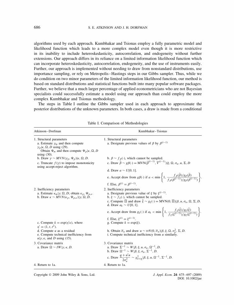
To see how the estimation technique employed here varies from the Bayesian technique presentedin Kumbhakar and Tsionas (2005), Table I presents a side-by-side comparison of the MCMC

5 The constants � and � could be estimated but that would greatly complicate the estimation algorithm by adding anumerical optimization step requiring a quasi-Newton or equivalent search algorithm for each loop through the Gibbssampler that will be employed to approximate the posterior. In return, one would get a more accurate marginal posteriordistribution for �. We choose to simply set the two constants to convenient values instead, given the interest is on asubset of the parameters in � .



algorithms used by each approach. Kumbhakar and Tsionas employ a fully parametric model andlikelihood function which leads to a more complex model even though it is more restrictivein its inability to include heteroskedasticity, autocorrelation, and endogeneity without furtherextensions. Our approach differs in its reliance on a limited information likelihood function whichcan incorporate heteroskedasticity, autocorrelation, endogeneity, and the use of instruments easily.Further, our approach is implemented without needing to draw from nonstandard distributions, useimportance sampling, or rely on Metropolis–Hastings steps in our Gibbs sampler. Thus, while wedo condition on two minor parameters of the limited information likelihood function, our method isbased on standard distributions and statistical functions built into many popular software packages.Further, we believe that a much larger percentage of applied econometricians who are not Bayesianspecialists could successfully estimate a model using our approach than could employ the morecomplex Kumbhakar and Tsionas methodology.

The steps in Table I outline the Gibbs sampler used in each approach to approximate theposterior distributions of the unknown parameters. In both cases, a draw is made from a conditional

Table I. Comparison of Methodologies

Atkinson–Dorfman Kumbhakar–Tsionas

1. Structural parameters 1. Structural parametersa. Estimate �m and then compute�pj, �, D using (29).

a. Designate previous values of ˇ by ˇ�i�1�

Obtain m and then compute pj, �, Dusing (30).b. Draw � ¾ MVN��p, p�j, �, D. b. ˇ ¾ fˇ�Ð�, which cannot be sampled.

c. Truncate f�� to impose monotonicityusing accept-reject algorithm.

c. Draw Q ¾ gˇ�Ð� D MVN�ˇ�i�1�

, V�i�1�

�j�, �, �u, u, , D

d. Draw a ¾ U[0, 1].

e. Accept draw from gˇ�Ð� if a < min

{1,

fˇ� Q �/gˇ� Q �fˇ�ˇ�i�1��/gˇ�ˇ�i�1��

}.

f. Else, ˇ�i� D ˇ�i�1�.

2. Inefficiency parameters 2. Inefficiency parametersa. Estimate mj�, �, D; obtain p, p, . a. Designate previous value of � by ��i�1�.b. Draw ¾ MVN�p, p,�j�, �, D. b. � ¾ f��Ð�, which cannot be sampled.

c. Compute � and draw Q� ¾ g��Ð� D MVN�0, ��jˇ, u, �u, �, , D.d. Draw ak ¾ U[0, 1].

e. Accept draw from g��Ð� if ak < min

{1,

f��Q��/g��Q��f��i�1��/g��i�1��

}.

f. Else, ��i� D ��i�1�.c. Compute k D exp��0�, where�0 D �1, t, t2�.

g. Compute k D exp��.

d. Compute u as a residual h. Obtain �u and draw u ¾ trN�0, �u�jˇ, �, �, �2u , , D.

e. Compute technical inefficiency fromuj�, , and D using (15).

i. Compute technical inefficiency from u similarly.

3. Covariance matrix 3. Covariance matrixa. Draw � ¾ IWj�, , D. a. Draw �1 ¾ Wjˇ, �, u, �u, ��1, D.

b. Draw ��1 ¾ Wjˇ, �, �u, �1, D.

c. Drawq C u0u

2�2u

¾ �2nCnjˇ, �, u, ��1, �1, D.

4. Return to 1a. 4. Return to 1a.



distribution in each step. When the end of the list of steps is reached, one returns to step 1 andrepeats. The draws form an empirical approximation to the joint posterior distribution.

For the Atkinson–Dorfman approach, the steps are slightly simplified in places. Since we define D fLf, L1t, L2t, Ef, E1t, E2tg, reference to drawing in Table I is actually a reference todrawing Lf, L1t, L2t, Ef, E1t, and E2t in six consecutive steps. Since we define � D ��d, �s�,reference to drawing � is actually a reference to drawing �d and then �s in two consecutive steps.Each consecutive step is conditional on the draws of the previous ones. We reiterate that � isthe covariance matrix of the error terms, �p is the posterior mean of � and p is its posteriorcovariance matrix. Similarly, p is the posterior mean of and p, is its posterior covariancematrix.

Using the notation in equation (11) of Kumbhakar and Tsionas (2005), their model is

y D X��ˇ C ��, υ� C � C(

u0�m�1�n

)�31�

Additionally, they define ˇ and V as the posterior mean and covariance for ˇ, while � and represent the covariance matrices for � and the error term, �, respectively. The parameters m andn are the number of share equations and observations, respectively. The scalar �u refers to thestandard deviation of u, which is distributed as half-normal, while n and q are hyperparametersfrom the prior on �u. Further, � represents a posterior covariance matrix for � and �u a posteriorvariance for u. Note that in place of our k, they employ � D in�k�. Finally, D represents the datain both approaches.

Based on this table, one can also see the simplicity of our method compared to that of Kumbhakarand Tsionas (2005) both in terms of the number of steps required and the distributional assumptionsrequired to obtain estimates of allocative and technical efficiency. Specifically, we avoid theirMetropolis–Hastings sampling in steps 1 and 2.

In step 3, we are required to draw from only one of three distributions that they draw from.Further, their approach requires that they discard the first 15,000 MCMC draws and use only thelast 5000. With our approach we quickly overcome starting value problems and keep the vastmajority of our draws.

3.4. Implementation of the Gibbs Sampler

A total of 12,000 Gibbs draws were generated from four separate chains. Each chain was 3500draws long, with the first 500 discarded to remove dependence on initial starting values (standardGMM estimates were used for that purpose). Convergence was checked by confirming the posteriormeans of the four separate chains were statistically equivalent. For example, the posterior meansand medians of the TE measures did not differ by more than 0.5% in any case across the chains.

We impose certain restrictions in order to achieve identification. First, we impose the restrictionˇ0 D 0 in (9), in order to identify the coefficients of the other plant-specific dummies, ˇf0, , 8f.Second, we restrict the allocative inefficiency parameters for one input to achieve identification ofthe others; this is done by setting knft D 1, 8t for one n.

Joint estimation of this system using GMM (which is a part of the formula for the posterior modeof our Bayesian estimator) requires that the model satisfy the moment conditions E�vftjzft� D 0,where zft is a vector of instruments. Although not strictly Bayesian, we report the standard



Hansen (1982) J-test of overidentifying restrictions to determine the validity of the instrument setthat is used to estimate our distance system using GMM. We fail to reject the null hypothesis thatthe moment conditions are satisfied when we employ the following instrument set: all plant-leveldummies, the interaction of an ‘older’ vintage variable (pre-1948 D 1) and log output, the log of thereal node price of electricity, a variable measuring the relative hydrologic conditions (water levelrelative to average water level), w, w2, w3, w4, t, t2, t3, the interaction of the run-of-river dummywith monthly dummies, the interaction of the logs of inputs and the log of output with time, theinteraction of the logs of inputs with w, log output, the interaction of the run-of-river dummy withoutput, and log output squared. We allow for heteroskedasticity and autocorrelation of unknownform by computing the consistent covariance matrix following Newey and West (1987) with 10monthly lags. The lag length was chosen in order the minimize the GMM criterion function. Basedon the J-test, we easily accept the null hypothesis of the validity of the overidentifying conditions.Because we must perform this test for each draw of our Gibbs sampler, results vary. However, wealways find a p-value in excess of 0.50 with 192 degrees of freedom in the step where we free upthe structural parameters. We find that the instruments are not weak based on a regression of eachendogenous variable on the list of instruments yielding F statistics greater than the rule-of-thumbvalue of 10.6

For the duality between input prices and quantities to be valid, the input shadow distancefunction must be monotonically increasing in inputs and monotonically decreasing in outputs. Ourestimated model satisfies the required monotonicity properties for inputs and outputs for at least99% and 95% of the data points, respectively (since that condition was imposed in estimation byrestricting draws to the region R).

4. DATA AND RESULTS

4.1. Data

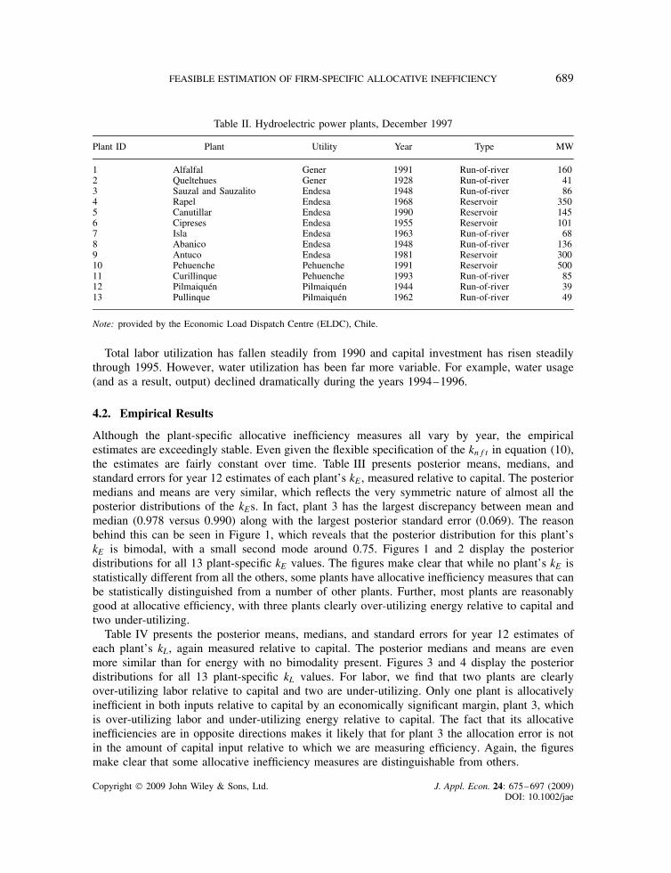
Our sample is a rotated and unbalanced panel, consisting of 13 Chilean hydroelectric power gen-eration plants, observed monthly for a maximum of 141 data points per plant spanning April 1986to December 1997. The monthly frequency is designed to capture the considerable variation inthe country’s hydrologic conditions throughout the year. Table II lists the 13 plants for whichwe have observations, their controlling firm, year of initial service, type of hydro generation,and MW capacity. The four controlling firms really constitute three—Endesa, Gener, and Pil-maiquen—since Endesa owns Pehuenche. Thus, our final sample consists of 13 plants (owned bythree firms) with a total of 1935 monthly observations. Observations per plant range from 49 to 141.

The panel was unbalanced for two reasons. The first and most important reason is the staggeredinitial in-rotation of plants following their construction. The second and less important reason isthe limited out-rotation by some plants due to plant-specific mechanical problems.

At the plant level, we record the output quantity (Q), the price per unit of output, and the priceand quantity of three inputs—labor (L), capital (K), and water (E)—which we also refer to asenergy. All the quantities and prices have been normalized by their means before taking theirlogarithms. Prices are all in real terms. Full details of the dataset can be found in Atkinson andHalabı (2004). We arbitrarily normalize kkft to 1 for all plants and time periods.

6 A variety of instrument sets were examined. Of these only a few passed the J-test. Among these, only minor differencesappeared in the final results.



Table II. Hydroelectric power plants, December 1997

Plant ID Plant Utility Year Type MW

1 Alfalfal Gener 1991 Run-of-river 1602 Queltehues Gener 1928 Run-of-river 413 Sauzal and Sauzalito Endesa 1948 Run-of-river 864 Rapel Endesa 1968 Reservoir 3505 Canutillar Endesa 1990 Reservoir 1456 Cipreses Endesa 1955 Reservoir 1017 Isla Endesa 1963 Run-of-river 688 Abanico Endesa 1948 Run-of-river 1369 Antuco Endesa 1981 Reservoir 30010 Pehuenche Pehuenche 1991 Reservoir 50011 Curillinque Pehuenche 1993 Run-of-river 8512 Pilmaiquen Pilmaiquen 1944 Run-of-river 3913 Pullinque Pilmaiquen 1962 Run-of-river 49

Note: provided by the Economic Load Dispatch Centre (ELDC), Chile.

Total labor utilization has fallen steadily from 1990 and capital investment has risen steadilythrough 1995. However, water utilization has been far more variable. For example, water usage(and as a result, output) declined dramatically during the years 1994–1996.

4.2. Empirical Results

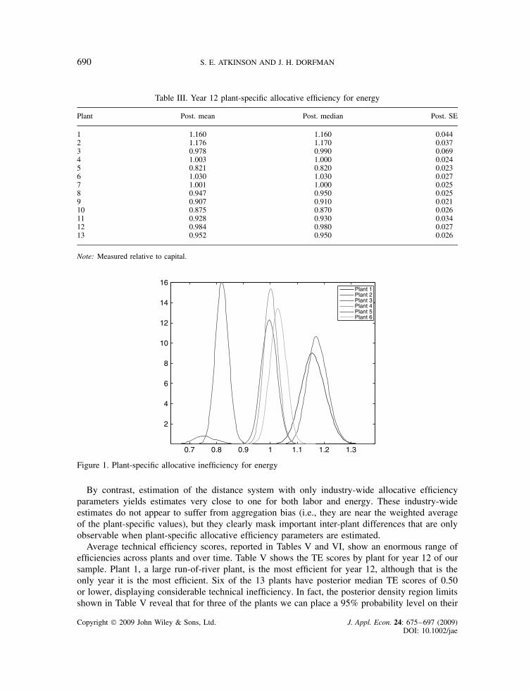
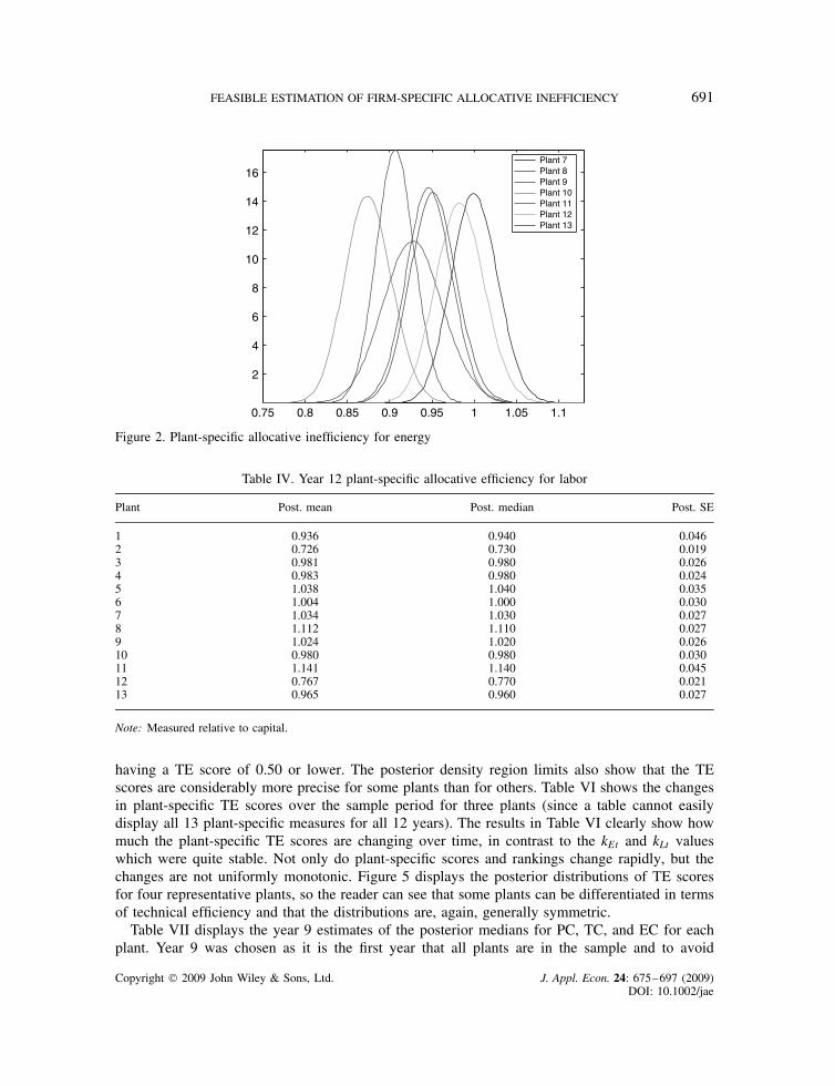
Although the plant-specific allocative inefficiency measures all vary by year, the empiricalestimates are exceedingly stable. Even given the flexible specification of the knft in equation (10),the estimates are fairly constant over time. Table III presents posterior means, medians, andstandard errors for year 12 estimates of each plant’s kE, measured relative to capital. The posteriormedians and means are very similar, which reflects the very symmetric nature of almost all theposterior distributions of the kEs. In fact, plant 3 has the largest discrepancy between mean andmedian (0.978 versus 0.990) along with the largest posterior standard error (0.069). The reasonbehind this can be seen in Figure 1, which reveals that the posterior distribution for this plant’skE is bimodal, with a small second mode around 0.75. Figures 1 and 2 display the posteriordistributions for all 13 plant-specific kE values. The figures make clear that while no plant’s kE isstatistically different from all the others, some plants have allocative inefficiency measures that canbe statistically distinguished from a number of other plants. Further, most plants are reasonablygood at allocative efficiency, with three plants clearly over-utilizing energy relative to capital andtwo under-utilizing.

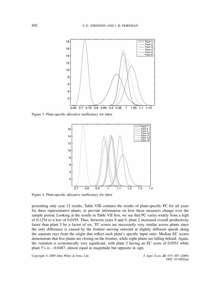
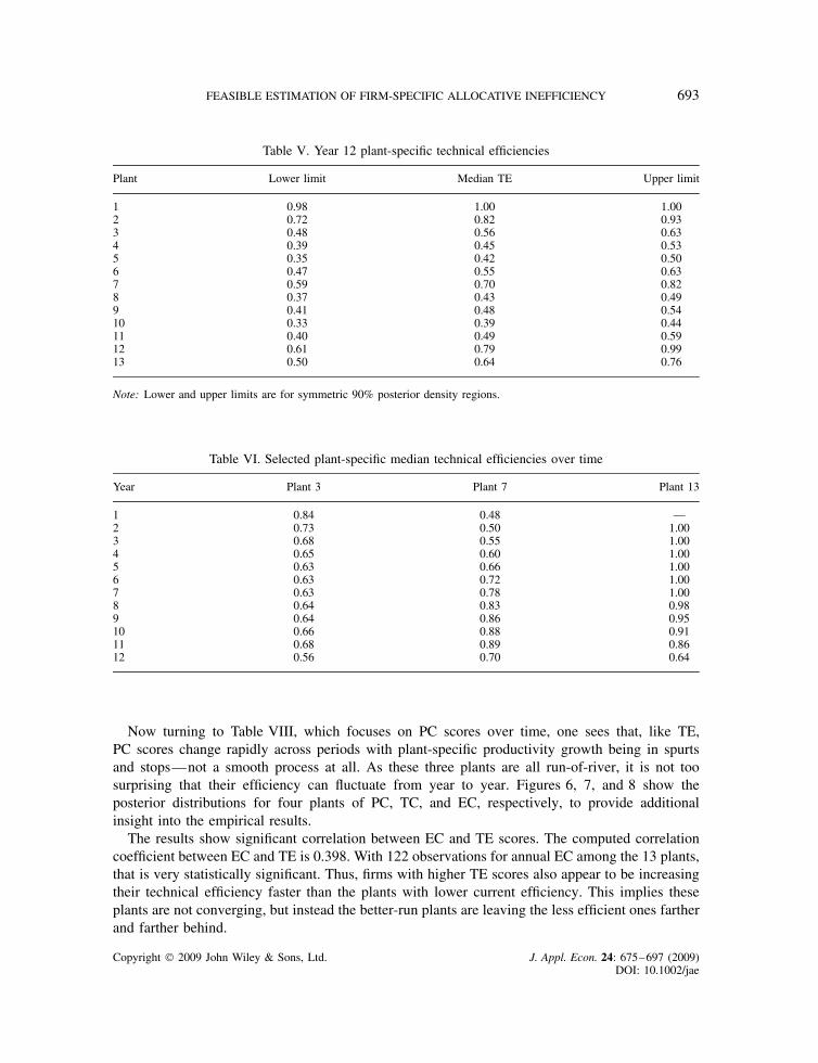
Table IV presents the posterior means, medians, and standard errors for year 12 estimates ofeach plant’s kL, again measured relative to capital. The posterior medians and means are evenmore similar than for energy with no bimodality present. Figures 3 and 4 display the posteriordistributions for all 13 plant-specific kL values. For labor, we find that two plants are clearlyover-utilizing labor relative to capital and two are under-utilizing. Only one plant is allocativelyinefficient in both inputs relative to capital by an economically significant margin, plant 3, whichis over-utilizing labor and under-utilizing energy relative to capital. The fact that its allocativeinefficiencies are in opposite directions makes it likely that for plant 3 the allocation error is notin the amount of capital input relative to which we are measuring efficiency. Again, the figuresmake clear that some allocative inefficiency measures are distinguishable from others.



Table III. Year 12 plant-specific allocative efficiency for energy

Plant Post. mean Post. median Post. SE

1 1.160 1.160 0.0442 1.176 1.170 0.0373 0.978 0.990 0.0694 1.003 1.000 0.0245 0.821 0.820 0.0236 1.030 1.030 0.0277 1.001 1.000 0.0258 0.947 0.950 0.0259 0.907 0.910 0.02110 0.875 0.870 0.02611 0.928 0.930 0.03412 0.984 0.980 0.02713 0.952 0.950 0.026

Note: Measured relative to capital.

0.7 0.8 0.9 1 1.1 1.2 1.3

2

4

6

8

10

12

14

16Plant 1Plant 2Plant 3Plant 4Plant 5Plant 6

Figure 1. Plant-specific allocative inefficiency for energy

By contrast, estimation of the distance system with only industry-wide allocative efficiencyparameters yields estimates very close to one for both labor and energy. These industry-wideestimates do not appear to suffer from aggregation bias (i.e., they are near the weighted averageof the plant-specific values), but they clearly mask important inter-plant differences that are onlyobservable when plant-specific allocative efficiency parameters are estimated.

Average technical efficiency scores, reported in Tables V and VI, show an enormous range ofefficiencies across plants and over time. Table V shows the TE scores by plant for year 12 of oursample. Plant 1, a large run-of-river plant, is the most efficient for year 12, although that is theonly year it is the most efficient. Six of the 13 plants have posterior median TE scores of 0.50or lower, displaying considerable technical inefficiency. In fact, the posterior density region limitsshown in Table V reveal that for three of the plants we can place a 95% probability level on their



0.75 0.8 0.85 0.9 0.95 1 1.05 1.1

2

4

6

8

10

12

14

16Plant 7Plant 8Plant 9Plant 10Plant 11Plant 12Plant 13

Figure 2. Plant-specific allocative inefficiency for energy

Table IV. Year 12 plant-specific allocative efficiency for labor

Plant Post. mean Post. median Post. SE

1 0.936 0.940 0.0462 0.726 0.730 0.0193 0.981 0.980 0.0264 0.983 0.980 0.0245 1.038 1.040 0.0356 1.004 1.000 0.0307 1.034 1.030 0.0278 1.112 1.110 0.0279 1.024 1.020 0.02610 0.980 0.980 0.03011 1.141 1.140 0.04512 0.767 0.770 0.02113 0.965 0.960 0.027

Note: Measured relative to capital.

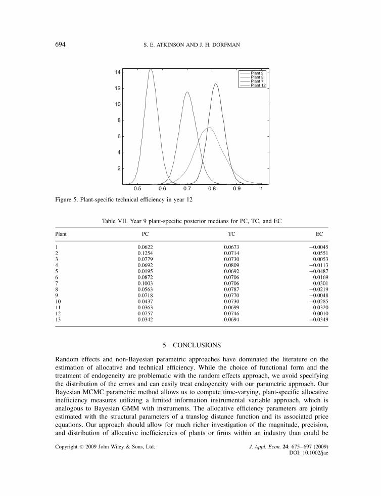
having a TE score of 0.50 or lower. The posterior density region limits also show that the TEscores are considerably more precise for some plants than for others. Table VI shows the changesin plant-specific TE scores over the sample period for three plants (since a table cannot easilydisplay all 13 plant-specific measures for all 12 years). The results in Table VI clearly show howmuch the plant-specific TE scores are changing over time, in contrast to the kEt and kLt valueswhich were quite stable. Not only do plant-specific scores and rankings change rapidly, but thechanges are not uniformly monotonic. Figure 5 displays the posterior distributions of TE scoresfor four representative plants, so the reader can see that some plants can be differentiated in termsof technical efficiency and that the distributions are, again, generally symmetric.

Table VII displays the year 9 estimates of the posterior medians for PC, TC, and EC for eachplant. Year 9 was chosen as it is the first year that all plants are in the sample and to avoid



0.65 0.7 0.75 0.8 0.85 0.9 0.95 1 1.05 1.1 1.15

2

4

6

8

10

12

14

16

18 Plant 1Plant 2Plant 3Plant 4Plant 5Plant 6

Figure 3. Plant-specific allocative inefficiency for labor

0.7 0.8 0.9 1 1.1 1.2 1.3 1.4

2

4

6

8

10

12

14

16Plant 7Plant 8Plant 9Plant 10Plant 11Plant 12Plant 13

Figure 4. Plant-specific allocative inefficiency for labor

presenting only year 12 results. Table VIII contains the results of plant-specific PC for all yearsfor three representative plants, to provide information on how these measures change over thesample period. Looking at the results in Table VII first, we see that PC varies widely from a highof 0.1254 to a low of 0.0195. Thus, between years 8 and 9, plant 2 increased overall productivityfaster than plant 5 by a factor of six. TC scores are necessarily very similar across plants sincethe only difference is caused by the frontier moving outward at slightly different speeds alongthe separate rays from the origin that reflect each plant’s specific input ratio. Median EC scoresdemonstrate that five plants are closing on the frontier, while eight plants are falling behind. Again,the variation is economically very significant, with plant 2 having an EC score of 0.0551 whileplant 5’s is �0.0487, almost equal in magnitude but opposite in sign.



Table V. Year 12 plant-specific technical efficiencies

Plant Lower limit Median TE Upper limit

1 0.98 1.00 1.002 0.72 0.82 0.933 0.48 0.56 0.634 0.39 0.45 0.535 0.35 0.42 0.506 0.47 0.55 0.637 0.59 0.70 0.828 0.37 0.43 0.499 0.41 0.48 0.5410 0.33 0.39 0.4411 0.40 0.49 0.5912 0.61 0.79 0.9913 0.50 0.64 0.76

Note: Lower and upper limits are for symmetric 90% posterior density regions.

Table VI. Selected plant-specific median technical efficiencies over time

Year Plant 3 Plant 7 Plant 13

1 0.84 0.48 —2 0.73 0.50 1.003 0.68 0.55 1.004 0.65 0.60 1.005 0.63 0.66 1.006 0.63 0.72 1.007 0.63 0.78 1.008 0.64 0.83 0.989 0.64 0.86 0.9510 0.66 0.88 0.9111 0.68 0.89 0.8612 0.56 0.70 0.64

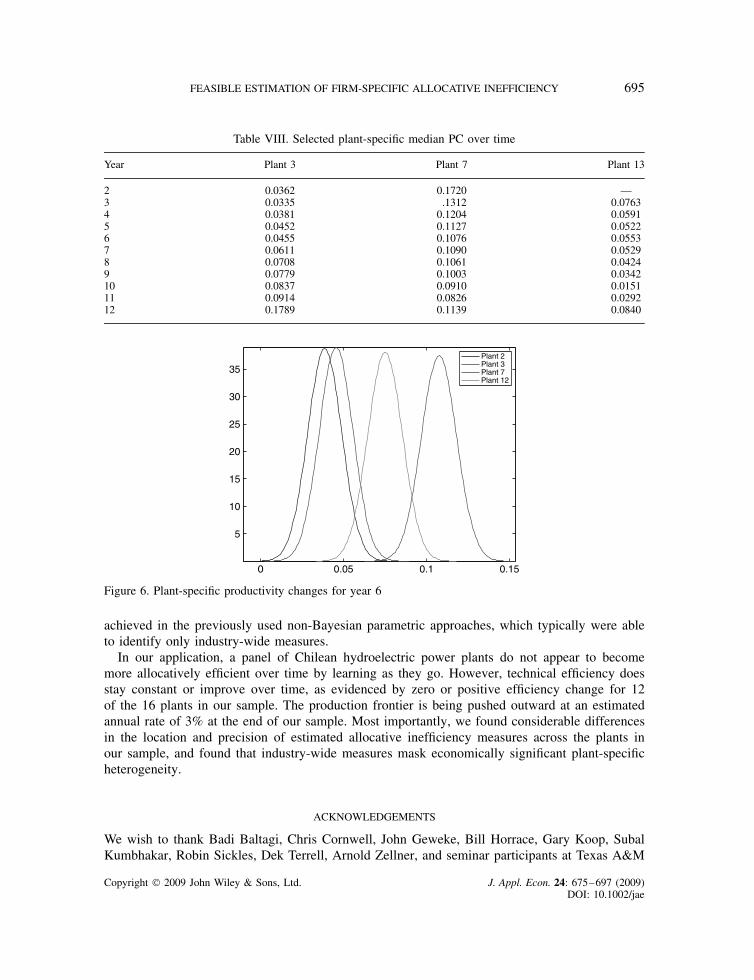
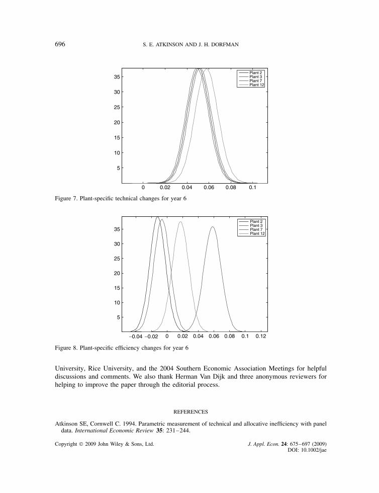
Now turning to Table VIII, which focuses on PC scores over time, one sees that, like TE,PC scores change rapidly across periods with plant-specific productivity growth being in spurtsand stops—not a smooth process at all. As these three plants are all run-of-river, it is not toosurprising that their efficiency can fluctuate from year to year. Figures 6, 7, and 8 show theposterior distributions for four plants of PC, TC, and EC, respectively, to provide additionalinsight into the empirical results.

The results show significant correlation between EC and TE scores. The computed correlationcoefficient between EC and TE is 0.398. With 122 observations for annual EC among the 13 plants,that is very statistically significant. Thus, firms with higher TE scores also appear to be increasingtheir technical efficiency faster than the plants with lower current efficiency. This implies theseplants are not converging, but instead the better-run plants are leaving the less efficient ones fartherand farther behind.



0.5 0.6 0.7 0.8 0.9 1

2

4

6

8

10

12

14 Plant 2Plant 3Plant 7Plant 12

Figure 5. Plant-specific technical efficiency in year 12

Table VII. Year 9 plant-specific posterior medians for PC, TC, and EC

Plant PC TC EC

1 0.0622 0.0673 �0.00452 0.1254 0.0714 0.05513 0.0779 0.0730 0.00534 0.0692 0.0809 �0.01135 0.0195 0.0692 �0.04876 0.0872 0.0706 0.01697 0.1003 0.0706 0.03018 0.0563 0.0787 �0.02199 0.0718 0.0770 �0.004810 0.0437 0.0730 �0.028511 0.0363 0.0699 �0.032012 0.0757 0.0746 0.001013 0.0342 0.0694 �0.0349

5. CONCLUSIONS

Random effects and non-Bayesian parametric approaches have dominated the literature on theestimation of allocative and technical efficiency. While the choice of functional form and thetreatment of endogeneity are problematic with the random effects approach, we avoid specifyingthe distribution of the errors and can easily treat endogeneity with our parametric approach. OurBayesian MCMC parametric method allows us to compute time-varying, plant-specific allocativeinefficiency measures utilizing a limited information instrumental variable approach, which isanalogous to Bayesian GMM with instruments. The allocative efficiency parameters are jointlyestimated with the structural parameters of a translog distance function and its associated priceequations. Our approach should allow for much richer investigation of the magnitude, precision,and distribution of allocative inefficiencies of plants or firms within an industry than could be



Table VIII. Selected plant-specific median PC over time

Year Plant 3 Plant 7 Plant 13

2 0.0362 0.1720 —3 0.0335 .1312 0.07634 0.0381 0.1204 0.05915 0.0452 0.1127 0.05226 0.0455 0.1076 0.05537 0.0611 0.1090 0.05298 0.0708 0.1061 0.04249 0.0779 0.1003 0.034210 0.0837 0.0910 0.015111 0.0914 0.0826 0.029212 0.1789 0.1139 0.0840

0 0.05 0.1 0.15

5

10

15

20

25

30

35Plant 2Plant 3Plant 7Plant 12

Figure 6. Plant-specific productivity changes for year 6

achieved in the previously used non-Bayesian parametric approaches, which typically were ableto identify only industry-wide measures.

In our application, a panel of Chilean hydroelectric power plants do not appear to becomemore allocatively efficient over time by learning as they go. However, technical efficiency doesstay constant or improve over time, as evidenced by zero or positive efficiency change for 12of the 16 plants in our sample. The production frontier is being pushed outward at an estimatedannual rate of 3% at the end of our sample. Most importantly, we found considerable differencesin the location and precision of estimated allocative inefficiency measures across the plants inour sample, and found that industry-wide measures mask economically significant plant-specificheterogeneity.

ACKNOWLEDGEMENTS

We wish to thank Badi Baltagi, Chris Cornwell, John Geweke, Bill Horrace, Gary Koop, SubalKumbhakar, Robin Sickles, Dek Terrell, Arnold Zellner, and seminar participants at Texas A&M



0 0.02 0.04 0.06 0.08 0.1

5

10

15

20

25

30

35Plant 2Plant 3Plant 7Plant 12

Figure 7. Plant-specific technical changes for year 6

−0.04 −0.02 0 0.02 0.04 0.06 0.08 0.1 0.12

5

10

15

20

25

30

35

Plant 2Plant 3Plant 7Plant 12

Figure 8. Plant-specific efficiency changes for year 6

University, Rice University, and the 2004 Southern Economic Association Meetings for helpfuldiscussions and comments. We also thank Herman Van Dijk and three anonymous reviewers forhelping to improve the paper through the editorial process.

REFERENCES

Atkinson SE, Cornwell C. 1994. Parametric measurement of technical and allocative inefficiency with paneldata. International Economic Review 35: 231–244.



Atkinson SE, Dorfman JH. 2005. Bayesian measurement of productivity and efficiency in the presence ofundesirable outputs: crediting electric utilities for reducing air pollution. Journal of Econometrics 126:445–468.

Atkinson SE, Halaba C. 2005. Measuring productivity growth and efficiency of the Chilean electric utilityindustry. Journal of Productivity Analysis 23: 245–273.

Atkinson SE, Halvorsen R. 1984. Parametric efficiency tests, economies of scale, and input demand in USelectric power generation. International Economic Review 25: 647–662.

Atkinson SE, Primont D. 2002. Measuring productivity growth, technical efficiency, allocative efficiency,and returns to scale using distance functions. Journal of Econometrics 108: 203–225.

Atkinson SE, Fare R, Primont D. 2003. Stochastic measurement of firm inefficiency using distance functions.Southern Economic Journal 69: 596–611.

Bauer PW. 1990. Recent developments in the econometric estimation of frontiers. Journal of Econometrics46: 39–56.

Casella G, George EI. 1992. Explaining the Gibbs sampler. American Statistician 46: 167–174.Cornwell C, Schmidt P, Sickles RC. 1990. Production frontiers with time series variation in efficiency levels.

Journal of Econometrics 46: 185–200.Greene WH. 1980. On the estimation of a flexible frontier production model. Journal of Econometrics 13:

101–115.Green E, Strawderman W. 1996. A Bayesian growth and yield model for slash pine plantations. Journal of

Applied Statistics 23: 285–299.Greene WH. 1997. Frontier production functions. In Handbook of Applied Econometrics. Vol. II: Microeco-

nomics , Pesaran MH, Schmidt P (eds). Blackwell: Oxford; 81–166.Griffin JE, Steel MFJ. 2004. Semiparametric Bayesian inference for stochastic frontier models. Journal of

Econometrics 123: 121–152.Hansen B. 1982. Large sample properties of generalized method of moments estimators. Econometrica 50:

1029–1054.Haung CJ, Liu JT. 1994. Estimation of a non-neutral atochastic frontier production function. Journal of

Productivity Analysis 5: 171–180.Kim JY. 2002. Limited information likelihood and Bayesian analysis. Journal of Econometrics 107: 175–193.Koop G, Poirier DJ. 2004. Bayesian variants of some classical semiparametric regression techniques. Journal

of Econometrics 123: 259–282.Koop G, Tobias JL. 2006. Semiparametric Bayesian inference in smooth coefficient models. Journal of

Econometrics 134: 283–315.Koop G, Osiewalski J, Steel FM. 1999. The components of output growth: a stochastic frontier analysis.

Oxford Bulletin of Economics and Statistics 61: 455–487.Kumbhakar SC, Tsionas EG. 2005. The joint measurement of technical and allocative inefficiencies: an

application of Bayesian inference in nonlinear random-effects models. Journal of the American StatisticalAssociation 100: 736–747.

LaFrance J. 1999. Inferring the nutrient content of food with prior information. American Journal ofAgricultural Economics 81: 728–734.

Lim H, Shumway CR. 1992. Profit maximization, returns to scale, and measurement error. Review ofEconomics and Statistics 74: 430–438.

Newey WK, West KD. 1987. A simple, positive semi-definite, heteroskedasticity and autocorrelation consis-tent covariance matrix. Econometrica 55: 703–706.

Tierney L. 1994. Markov chains for exploring posterior distributions (with discussion). Annals of Statistics22: 1701–1762.

Zellner A. 1998. The finite sample properties of simulataneous equations? Estimates and estimators: Bayesianand non-Bayesian approaches. Journal of Econometrics 83: 185–212.

Zellner A, Highfield RA. 1988. Calculation of maximum entropy distributions and approximation of marginalposterior distributions. Journal of Econometrics 37: 195–209.

Zellner A, Tobias J. 2001. Further results on Bayesian method of moments analysis of the multiple regressionmodel. International Economic Review 42: 121–140.

Zellner A, Bauwens L, Van Dijk HK. 1988. Bayesian specification analysis and estimation of simultaneousequation models using Monte Carlo methods. Journal of Econometrics 38: 39–72.
