MEASURING TECHNICAL AND ALLOCATIVE INEFFICIENCY

IN THE TRANSLOG COST SYSTEM: A BAYESIAN APPROACH*

Subal C. Kumbhakar Department of Economics

State University of New York Binghamton, NY 13902, USA.

Phone: (607) 777 4762, Fax: (607) 777 2681 E-mail: kkar@binghamton.edu

and

Efthymios G. Tsionas

Department of Economics Athens University of Economics and Business

76 Patission Street, 104 34 Athens, Greece. Phone: (301) 0820 3388, Fax: (301) 0820 3310

E-mail: tsionas@aueb.gr

Abstract

In this paper we propose simulation based Bayesian inference procedures in a cost system that includes the cost function and the cost share equations augmented to accommodate technical and allocative inefficiency. Markov Chain Monte Carlo techniques are proposed and implemented for Bayesian inferences on costs of technical and allocative inefficiency, input price distortions and over- (under-) use of inputs. We show how to estimate a well-specified translog system (in which the error terms in the cost and cost-share equations are internally consistent) in a random effects framework. The new methods are illustrated using panel data on U.S. commercial banks.

JEL classification: C11, C13

Key Words: Technical efficiency, translog cost function system, Markov Chain Monte Carlo techniques, panel data, nonlinear random effect models and commercial banks. * This paper was presented at the conference on “Current Developments in Productivity and Efficiency Measurement,” University of Georgia, October 25-26, 2002. We would like to thank Gary Koop, three anonymous referees and the participants of the conference for their valuable comments. We, alone, are responsible for any remaining errors.

1. Introduction

Empirical estimation of efficiency in the stochastic frontier (SF) models (developed by Aigner,

Lovell and Schmidt (1977) and Meeusen and van den Broeck (1977)) involve estimation of a parametric

production/cost/profit function with a composed error term consisting of a two-sided disturbance term

that reflects exogenous shocks and a one-sided term that captures technical inefficiency.1 Although the

theory is well developed to estimate a system of equations either in the form of factor demand or cost

function and cost share equations, the system approach is rarely applied in the efficiency literature.2 The

reason is that the error structure comprising noise, technical and allocative inefficiency complicates

econometric estimation of the model. This is especially the case when one uses flexible functional forms

to represent the underlying technology.3 Joint estimation of technical and allocative inefficiency in a

translog cost function presents a difficult problem (Greene (1980)).4 The difficulty is that the cost

function and the deviations of optimal shares from observed shares are complicated functions of

allocative inefficiency. Although many attempts have been proposed, none have been entirely successful.

Recently Kumbhakar (1997) proposed a solution for the Greene problem using a translog cost system, but

empirical estimation of this model has been restricted to panel data models in which technical and

allocative inefficiency are either assumed to be fixed parameters or functions of the data and unknown

parameters (Atkinson and Cornwell (1994); Maietta (2000)). In this paper, we show that relatively simple

econometric tools can be used to estimate technical and allocative inefficiency and perform exact

inference in this model without assuming technical and allocative inefficiency as fixed parameters. Thus

the main contribution of the paper is to show how to estimate a well-specified translog system (in which

the error terms in the cost and cost-share equations are internally consistent) in a random effects

framework.

More specifically, here we consider a Bayesian approach to address the Greene problem.

Bayesian analysis of a stochastic frontier function was first proposed by van den Broeck, Koop,

Osiewalski, and Steel (1994). The Gibbs sampler has been proposed as an effective numerical technique

by Koop, Steel, and Osiewalski (1995) where it is shown that Gibbs sampling has an advantage over

importance sampling. Koop, Osiewalski, and Steel (1997) proposed measuring technical inefficiency in

panel data models where technical inefficiency is time-invariant. Fernandez, Koop, and Steel (2000)

1 For a review of the efficiency literature see Bauer (1990), Greene (1993, 2001), Kumbhakar and Lovell (2000), and Koop and Steel (2001). 2 On the contrary, estimation of a cost system is a common practice when measurement of input elasticities, returns to scale, productivity growth, etc., are sought (see, for example, Christensen and Greene (1976), Diewert and Wales (1987)). 3 System approach with self-dual production function is used in Schmidt and Lovell (1979, 1980), Kumbhakar (1987), Kumbhakar et al. (1991), among many others. 4 It is now labeled in the literature as the Greene problem (see Bauer (1990)). For a simpler functional form such as the Cobb-Douglas it is not a problem (see Schmidt and Lovell (1979)).

1

considered Bayesian estimation of a system of equations involving a multi-output production function

without an explicit behavioral assumption (such as cost minimization or revenue/profit maximization).

Here we consider a system approach that is derived from a translog cost function and the cost share

equations. Thus, a cost minimization assumption is formally introduced in our model. We propose a

Bayesian approach to estimate the translog cost system with only technical inefficiency, first. This model

is different from the single equation cost function model of Koop et al. (1997). We then consider the cost

system, in which both technical and allocative inefficiency are present. Although the former model is

nested in the latter, estimation of the latter model is not a trivial extension of the former. Specialized

numerical methods are needed to provide parameter inferences and measures of technical and allocative

inefficiency.

We show that numerical analysis of the model from the Bayesian perspective can be facilitated

using Markov Chain Monte Carlo (MCMC) procedures. Posterior analysis of the model resembles many

features of the standard posterior analysis in the context of multivariate regression models. Exact finite

sample posterior distributions are provided without resorting to asymptotic approximations. To account

for the parametric restrictions across equations, we construct a semi-informative prior that allows for

differing degrees of “correctness” of the restrictions. We also provide tools for efficiency measurement in

both with and without allocative inefficiency models. Allocative inefficiency is modeled via price

distortions from which inferences are drawn on input over- (under-) use. In other words, we draw (firm-

specific) inferences on both price distortions and input over- (under-) use along with technical efficiency.

The new methods are illustrated using panel data on U.S. commercial banks.

The remainder of the paper is organized as follows. The model with only technical inefficiency is

developed in Section 2. This is followed by the model in which both technical and allocative inefficiency

are modeled jointly. Section 4 deals with prior specification. The U.S. commercial banking data and

empirical results are discussed in Section 5 while Section 6 concludes the paper.

2. A model with only technical inefficiency

We begin with a cost minimizing behavior where firms are allocatively efficient. Assuming that

panel data is available and technical inefficiency is time-invariant, the cost system can be written as

(Kumbhakar and Lovell (2000, p.155)

iititait uvCC ++= 0lnln , i , n,...,1= Tt ,...,1= (1)

itjitja

itj vSS ,0,, += , (2) Mj ,...,2=

2

where is the actual/observed cost of firm in year , is the observed cost share of input

( ), is the cost frontier (cost without technical and allocative inefficiencies) and is the

frontier cost share

aitC

M,...,

i t aitjS , j

j 1= 0itC 0

,itjS

5 of input , are the noise components, and is time-invariant technical

inefficiency, which can be interpreted as the percentage increase in cost due to technical inefficiency.

j itv 0≥iu

van den Broeck et al. (1994) and Koop et al. (1997) considered the cost function with time-

invariant inefficiency that is modeled above in a Bayesian framework. However, they used a single

equation approach and focused on estimating technical efficiency from the cost function alone. Another

feature of the model (in (1) and (2)) is that it resembles a seemingly unrelated regression (SUR) model. A

careful examination of the model reveals that it is also different from both the Fernandez, Koop, and Steel

(2000) model and the SUR model. We extend the Koop et al. model to a system and the SUR model to

accommodate technical inefficiency. Neither the technique proposed by Koop et al. (1997) and Fernandez

et al. (2000) nor the standard Bayesian SUR technique (Griffiths (2001)) can be applied to estimate the

model proposed above. Fernandez et al. (2000) present a system of equations associated with the distance

function but the formulation is ad hoc. Also, the numerical techniques presented here are different from

those in Fernandez et al. (2000).

We rewrite the above cost system in a generic form (which is a panel version of the SUR equation

system extended to include time-invariant technical inefficiency):

(3)

MMMM

T

vβXy

vβXyuvβXy

+=

+=⊗++=

2222

1111 1

where is an vector of observationsmy 1×nT 6 for the mth dependent variable ( = 1,…,m M ), is an

matrix of observations for the explanatory variables in the m

mX

mknT × th equation, mβ is a 1×mk

parameter error, is an random vector, is a mv 1×nT u 1×n non-negative random vector representing

time invariant technical inefficiency, and 1 is a T 1×T unit vector. Thus, n is the number of firms and

each of these firms is observed for T time periods. The first equation in (3) is the translog cost function,

and the remaining 1−M equations are the associated cost share equations. We rewrite (3) as

5 One cost share equation is dropped to avoid a singularity problem. 6 It is straightforward to accommodate unbalanced panels. We assume technical inefficiency is time invariant.

3

⊗++=

− )1(01

MnT

TuvXy β (4)

where is an vector of zeros, and the notations y and X are obvious. Regarding

stochastic components we assume that

)1(0 −MnT 1)1( ×−MnT

(i) v , where ),0(~ nTnTMnTM IN ⊗Σ Σ is an MM × contemporaneous covariance matrix;

(ii) u , i.e., u follows a half-normal distribution,),...,1(0,),0(~ 2 niuIN iui =≥σ 7

(iii) v and are mutually independent, as well as independent of u X .

With the above distributional assumptions the likelihood function of the model in (4) is given by

udupuAtrXyLn

un

u ∫+ℜ

−−− Σ−Σ∝Σ )()),((exp||),;,,( 1212/11 σβσβ (5)

where

nuu uuuup

u

n

+

−

ℜ∈′−

= ,)(exp

2)( 2

2

212σ

σπσ (6)

is the joint density function of u from (ii) above and

−′−⊗−−′−

−′⊗−−⊗−−′⊗−−=

)()()1()(

)()1()1()1(),(

111

111111111

MMMMMMTMMM

MMMTTT

XyXyuXyXy

XyuXyuXyuXyuA

ββββ

βββββ (7)

For a Bayesian analysis we need to choose the prior density function of the parameters, viz.,

Here we choose the following conditional structure: .),,( 1up σβ −Σ

)()()()()(),(),,( 1111uuuu ppppppp σβσσβσβ −−−− Σ∝ΣΣ∝Σ (8)

where

0,0,2

exp)( 2)1( ≥≥

−∝ +− qn

qp

u

nuu σ

σσ (9)

7 Other distributions such as the exponential, truncated normal and gamma could be used. The relevance of these distributions in practical applications is an issue worth exploring in future research.

4

( )121

2/)]1([11 exp)( −Σ

+−−− Σ−Σ∝Σ Σ trApMν

(10)

In (8) we assume, a priori, that β , Σ and uσ are independent. The prior on σ in (9) is inverted gamma.

The prior for in (10) is Wishart with parameters

2u

1−Σ Σν and . It reduces to the diffuse prior used by

Zellner (1971, p. 242) when

ΣA

0=Σν and MM×AΣ = 0 . Regarding the prior on β , )(βp , we choose a form

that can impose linear restrictions among the elements of β (that are derived from mathematical

properties of the cost function). A suitable candidate for this is the semi-informative prior of Geweke

(1993), i.e.,

H)(g,N~G q β (11)

where is a matrix (where is the total number of parameters and the rank of G kq× ∑=

=M

mmkk

1qG= ),

g is a vector, and 1×q H is a matrix whose inverse exists. When , the prior in (11)

allows exact imposition of the q linear restrictions. This is, indeed, the case here because the cost

function we are estimating satisfies some mathematical properties that are exact (see, for example,

Diewert (1982) for the properties of the cost function). As the elements of H diverge from , the prior

becomes increasingly vague. As

q×q qqH ×→ 0

qq×0

∞→H , the prior becomes improper.

2.1 Bayesian Inference

In sampling theory one starts computing the multiple integral in (5) and maximizes the likelihood

function with respect to the parameters. Although the multiple integral in the likelihood function (5) can

be computed analytically, it is likely that the log-likelihood function will be prone to numerical problems.

The same problems will be encountered in the Bayesian analysis of the posterior density function

when the latent variables are explicitly integrated out. This approach is called data augmentation. To

get around such problems, we consider the posterior density function (the product of (5) and (8))

augmented by the latent inefficiency variables :

u

u

)()()(

2exp)),(

21exp(),,,,(

1

2)1(12

)1(11

u

u

nnu

Mn

u

ppp

uuquAtrXyup

σβ

σσβσβ

−

++−−+−

−−

Σ×

′+−⋅Σ−Σ∝Σ

(12)

5

In (12) the latent variables are treated as parameters in order to avoid the complicated likelihood

function or posterior density function. This procedure facilitates considerably the use of MCMC

techniques that will be used to perform inferences for this model, as we explain later. In the sampling-

theory framework, this construction can be used to implement an EM algorithm.

u

Numerical Bayesian inference is performed using MCMC techniques8, especially the Gibbs

sampler. The philosophy of the method is simple. Given a posterior density function )|( Yp θ where

],...,[ 1 ′= pθθθ is the parameter vector, the objective is to simulate random draws Ss ,...,1=s ,)(θ from

the posterior. Once this is done the estimation problem is solved because (under quadratic loss) we can

estimate θ from ∑=

−=S

s

sS1

)(1 θθ and we can compute second or other moments in a similar way, if they

exist. We consider kernel densities of the individual elements of Sss ,...,1,)( =θ to form approximations

to marginal posterior density functions of parameters. The same is true for any function )(θf of the

parameter vector, since we have the draws Ssf s ,...,1),( )( =θ . To generate draws from the posterior

density function )|( Yp θ we consider the conditional density functions )Y,j|(p j −θθ ( where ),...,1 p=j

j−θ denotes all elements of θ except the j th element. The sequence S,...,ss ,)( =θ 1 so generated is

called Gibbs sampling sequence (Gelfand and Smith (1990), Tanner and Wong (1987)) and it converges

in distribution to the posterior under fairly mild conditions (Roberts and Smith (1994)). This means that if

the number of draws is large, then one can use the draws Ss ,...,1=s ,)(θ as a sample from the posterior

density function.

In the present model we generate random drawings from the following conditionals:

(i) datauu ,,,| σβ Σ , (ii) datauu ,,,| σβΣ , (iii) datauu ,,,| Σβσ , and (iv) u datau ,,,| σβ Σ . We repeat this

cycle S times to generate a sequence of length S for each one of these parameters. The draws so generated

can be considered as a sample from the joint posterior density function of the parameters. The required

conditional density functions to implement Gibbs sampling are as follows. For the regression parameters

we have:

) ,(~,,,,1 VNXyu ku βσβ −Σ (13)

where the conditional posterior mean is

6

]))(([])([ 11111 gHGUyIXGHGXIX nTnT−−−−− ′+−⊗Σ′′+⊗Σ′=β ,

and the conditional posterior covariance matrix is

⊗=

− )1(01

MnT

TuU

111 ])([ −−− ′+⊗Σ′= GHGXIXV nT .

The conditional posterior density function of 1−Σ is:

)]),([exp(||),,,,( 1212

)1(11 −

Σ

+−+−− Σ+−Σ∝Σ

Σ

uAAtrXyuPMn

u βσβν

(14)

which is a Wishart density function. The conditional posterior density function of is: uσ

( )

+′−∝Σ ++−−

211

2exp|

u

)n(nuu

quu,u,y,Xβ,p

σσσ (15)

which implies

212 ~,,,, nnu

Xyuquu

+−Σ

+′χβ

σ. (16)

It can be shown that the conditional posterior density function of latent inefficiencies is given by

niuNXyu iiui ,...,1,0 ),,(~,,,, 2*

*1

1 =≥Σ− σµσβ (17)

where

∑=

==m

j

jjii nieT

1

12*

* ,...,1,σσµ ; 211

22* 1 u

u

T σσσ

σ+

= ; ,],..,[ 1 ′=−= mTmmmmm eeXye β ∑=

−=T

tmtm eTe

1

1

with ],...,[ 1 ′= mnmm eee

][ ijσ=

for . The inverse contemporaneous covariance matrix is expressed as

. Finally, the u 's are independent in (17). To derive this result, notice that from (12) we can

decompose the posterior as , in which the second part is

irrelevant. We follow the technique presented in Tsionas (1999) to draw from (17). This technique utilizes

acceptance sampling based on an exponential blanketing density whose parameter is chosen to maximize

the acceptance rate.

Mm ,..,1=

,|(up β Σ

1Σ−i

),|,,(),,, 11 XypXy uu σβσ −− Σ⋅

8 For a review of MCMC methods in econometrics, see Geweke (1999).

7

To set up the Gibbs sampler we draw random numbers from conditional posterior density

functions (13), (14), (15), (16) and (17). This task is straightforward because these density functions are

from well-known families like the normal, truncated normal and Wishart. Therefore, the Gibbs sampler

provides a straightforward numerical approach to Bayesian analysis of a translog cost system involving

technical inefficiency.

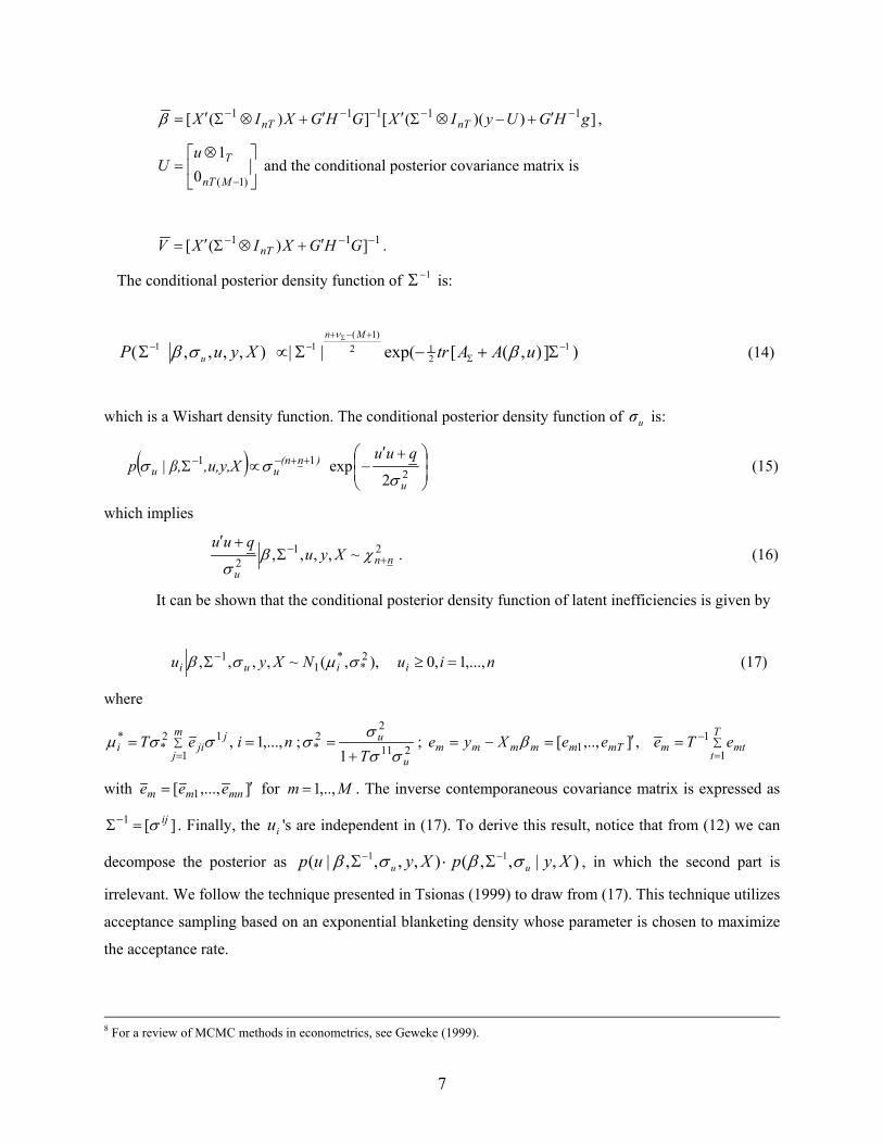
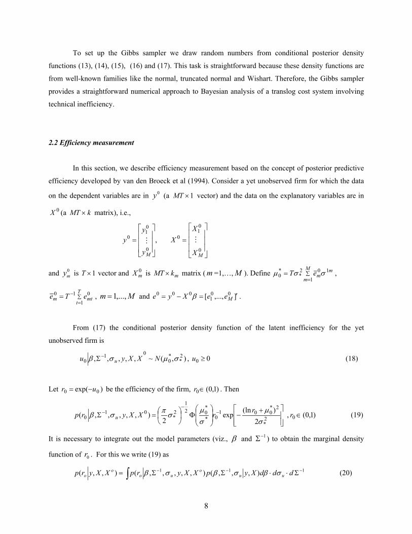
2.2 Efficiency measurement

In this section, we describe efficiency measurement based on the concept of posterior predictive

efficiency developed by van den Broeck et al (1994). Consider a yet unobserved firm for which the data

on the dependent variables are in (a 0y 1×MT vector) and the data on the explanatory variables are in

0X (a matrix), i.e., kMT ×

=

=0

01

0

0

01

0 ,

MM X

XX

y

yy

and is 0my 1×T vector and is MT0

mX mk× matrix ( =1,…,m M ). Define ∑=

=M

m

mmeT

1

102*

*0 σσµ ,

∑=

−=T

tmtm eTe

1

010 , and . Mm ,...,1= ],...,[ 001

000 ′=−= MeeXye β

From (17) the conditional posterior density function of the latent inefficiency for the yet

unobserved firm is

),(~,,,,, 2*

*0

010 σµσβ NXXyu u

−Σ , u (18) 00 ≥

Let be the efficiency of the firm, )exp( 00 ur −= )1,0(0∈r . Then

+−

Φ

=Σ −

−−

2*

2*001

0*

*02

1

2*

010 2

)(lnexp2

),,,,,(σµ

σµ

σπσβrrXXyrp u , (19) )1,0(0 ∈r

It is necessary to integrate out the model parameters (viz., β and 1−Σ ) to obtain the marginal density

function of . For this we write (19) as 0r

111 ),,,(),,,,,(),,( −−− Σ⋅⋅ΣΣ= ∫ dddXypXXyrpXXyrp uuo

uoo

o σβσβσβ (20)

8

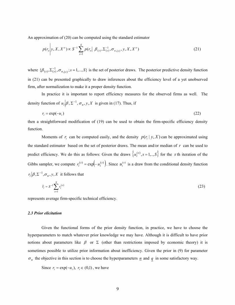
An approximation of (20) can be computed using the standard estimator

),,,,,(),,( )(,1)()(

1

1 osuss

S

so

oo XXyrpSXXyrp σβ −

=

− Σ∝ ∑ (21)

where is the set of posterior draws. The posterior predictive density function

in (21) can be presented graphically to draw inferences about the efficiency level of a yet unobserved

firm, after normalization to make it a proper density function.

,...,1;,, ),(1)()( Sssuss =Σ− σβ

In practice it is important to report efficiency measures for the observed firms as well. The

density function of Xyui ,,,, 1 σβ −Σu is given in (17). Thus, if

)exp( ii ur −= (22)

then a straightforward modification of (19) can be used to obtain the firm-specific efficiency density

function.

Moments of r can be computed easily, and the density can be approximated using

the standard estimator based on the set of posterior draws. The mean and/or median of

i ),|( Xyrp i

r can be used to

predict efficiency. We do this as follows: Given the draws Ss ,..,1,) =u si( for the th iteration of the

Gibbs sampler, we compute

s

( ))()( exp si

si ur −= . Since is a draw from the conditional density function )(s

iu

Xyr ui ,,,, 1 σβ −Σ it follows that

∑=

−=S

s

sii rSr

1

)(1 (23)

represents average firm-specific technical efficiency.

2.3 Prior elicitation

Given the functional forms of the prior density function, in practice, we have to choose the

hyperparameters to match whatever prior knowledge we may have. Although it is difficult to have prior

notions about parameters like β or Σ (other than restrictions imposed by economic theory) it is

sometimes possible to utilize prior information about inefficiency. Given the prior in (9) for parameter

uσ the objective in this section is to choose the hyperparameters n and q in some satisfactory way.

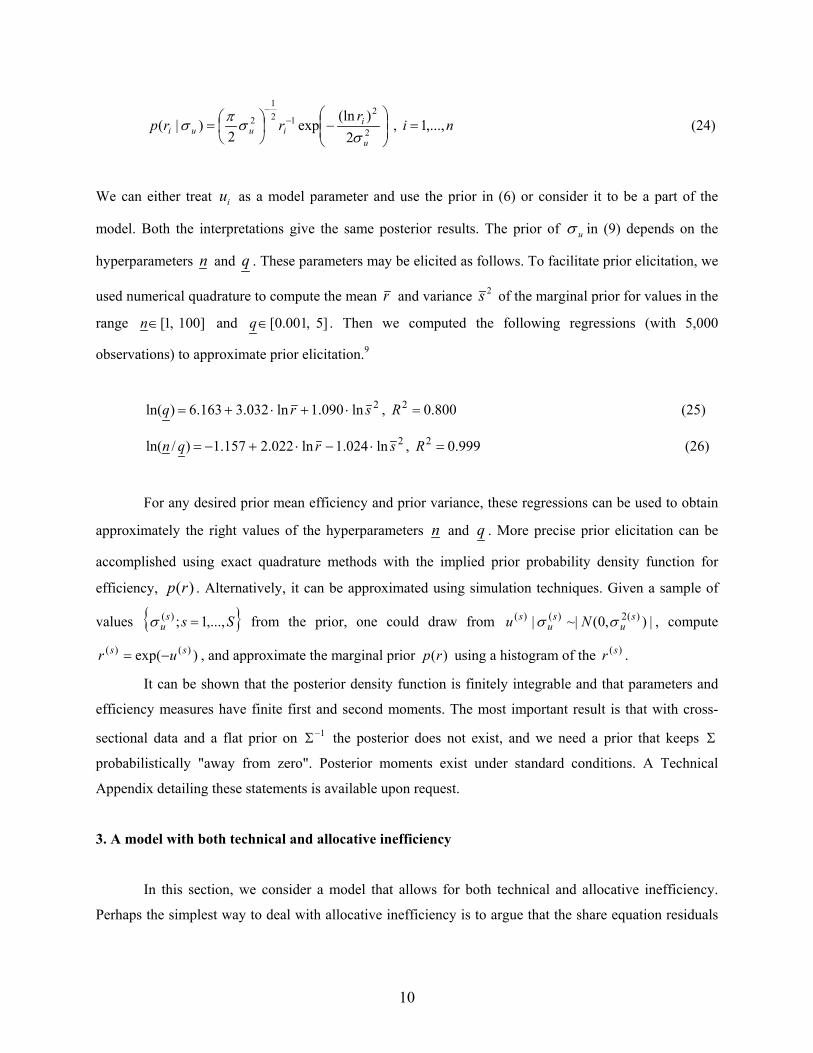
Since , we have )1,0(),exp( ∈−= iii rur

9

−

= −

−

2

212

1

2

2)(lnexp

2)|(

u

iiuui

rrrpσ

σπσ , i n,...,1= (24)

We can either treat u as a model parameter and use the prior in (6) or consider it to be a part of the

model. Both the interpretations give the same posterior results. The prior of

i

uσ in (9) depends on the

hyperparameters n and q . These parameters may be elicited as follows. To facilitate prior elicitation, we

used numerical quadrature to compute the mean r and variance 2s of the marginal prior for values in the

range ]100 ,1[∈n and ]5 ,001.0[∈q . Then we computed the following regressions (with 5,000

observations) to approximate prior elicitation.9

2ln090.1ln032.3163.6)ln( srq ⋅+⋅+= , (25) 800.02 =R

2ln024.1ln022.2157.1)/ln( srqn ⋅−⋅+−= , (26) 999.02 =R

For any desired prior mean efficiency and prior variance, these regressions can be used to obtain

approximately the right values of the hyperparameters n and q . More precise prior elicitation can be

accomplished using exact quadrature methods with the implied prior probability density function for

efficiency, . Alternatively, it can be approximated using simulation techniques. Given a sample of

values

)(rp

S,...,1σ

exp(

ssu ;)( =

))(su−

from the prior, one could draw from , compute

, and approximate the marginal prior using a histogram of the

|),0(~|| )(2)()( su

su

s Nu σσ

)(s)(sr = )(rp r .

It can be shown that the posterior density function is finitely integrable and that parameters and

efficiency measures have finite first and second moments. The most important result is that with cross-

sectional data and a flat prior on the posterior does not exist, and we need a prior that keeps 1−Σ Σ

probabilistically "away from zero". Posterior moments exist under standard conditions. A Technical

Appendix detailing these statements is available upon request.

3. A model with both technical and allocative inefficiency

In this section, we consider a model that allows for both technical and allocative inefficiency.

Perhaps the simplest way to deal with allocative inefficiency is to argue that the share equation residuals

10

represent deviations from first-order conditions and, therefore, they represent allocative distortions. This

modeling approach, however, fails to take into account the link between allocative inefficiency and its

impact on cost. Here we follow Kumbhakar (1997) who, following the definition of allocative

inefficiency from Schmidt and Lovell (1979), derived the exact relationship between allocative

inefficiency and cost therefrom in the context of the translog cost function. It solves the Greene problem

theoretically. No estimation technique is, however, offered. And we are not aware of any application

where the Greene problem is solved using a flexible cost function and treating allocative inefficiency as

random. In a sampling theory framework empirical application of the Kumbhakar (1997) model is

difficult because of the computational complexity of the model, especially when allocative inefficiency is

represented by random variables à la Schmidt and Lovell (1979).

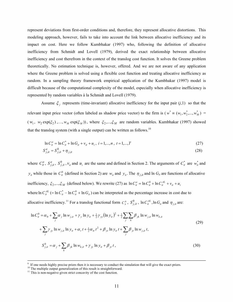
Assume jξ represents (time-invariant) allocative inefficiency for the input pair (j,1) so that the

relevant input price vector (often labeled as shadow price vector) to the firm is ( =

( ,

≡*w ),...,,( **21 Mwww

1w )exp( 22 ξw ,…, ))exp( MMw ξ , where Mξξ ,...,2 are random variables. Kumbhakar (1997) showed

that the translog system (with a single output) can be written as follows.10

iitititait uvGCC +++= lnlnln * , ni ,...,1= , t T,...,1= (27)

(28) itjitja

itj SS ,0,, η+=

where , , , and u are the same and defined in Section 2. The arguments of C are and

while those in (defined in Section 2) are and The

aitC a

itjS ,0,itjS

0itC

itv i*it

*itw

ity itw .ity itj,η and ln Git are functions of allocative

inefficiency, Mξξ ,...,

ln *itC

2

(AL =

(defined below). We rewrite (27) as ln

where can be interpreted as the percentage increase in cost due to

allocative inefficiency.

iitALitit uvCCC +++ ln0

0,jS it

ALit GC ln, itj ,η

ait = ln

it

)0ititit GC ln+ln−ln C

11 For a translog functional form , , ln and are: 0itC

( )

,lnlnlnln

lnlnlnlnlnln

,2

21

,

,,212

21

,00

twtyttyw

wwyywC

itjj

jtityttttj

ititjjy

j jitkitjjkityyityitjjit

∑∑

∑ ∑∑

+++++

++++=

ββααγ

βγγααk

(29)

tywS jtk

itjyitkjkjitj βγβα +++= ∑ lnln ,0, , (30)

9 If one needs highly precise priors then it is necessary to conduct the simulation that will give the exact priors. 10 The multiple output generalization of this result is straightforward. 11 This is non-negative given strict concavity of the cost function.

11

tywGC ijj

jtj

itijjyj k

ikijjkj j k

itkijjkijjitALit ,,,,2

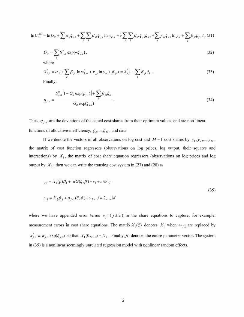
1,,, lnlnlnln ξβξγξξβξβξα ∑∑∑∑∑ ∑∑ +++++= , (31)

∑ −=j

ijitjit SG )exp( ,*, ξ , (32)

where

∑∑ +≡+++=k

kjkitjjtk

itjyitkjkjitj StywS ξββγβα 0,

*,

*, lnln . (33)

Finally,

)exp(

)exp(1

,

,0,

,ijit

kkjkijititj

itj G

GS

ξ

ξβξη

∑+−= . (34)

Thus, itj,η are the deviations of the actual cost shares from their optimum values, and are non-linear

functions of allocative inefficiency, Mξξ ,...,2 , and data.

If we denote the vectors of all observations on log cost and 1−M cost shares by ,

the matrix of cost function regressors (observations on log prices, log output, their squares and

interactions) by , the matrix of cost share equation regressors (observations on log prices and log

output by , then we can write the translog cost system in (27) and (28) as

Myyy ,...,, 21

1X

2X

TuvGXy 1),(ln)( 1111 ⊗+++= βξβξ

(35)

jjjj vXy ++= − ),(12 βξηβ , Mj ,...,2=

where we have appended error terms v ( 2j ) in the share equations to capture, for example,

measurement errors in cost share equations. The matrix

j ≥

)(1 ξX denotes when are replaced by

so that

1X itjw ,

)exp( ,,*

, ijitjitj ww ξ≡ 1X11 )0(X M =− . Finally, β denotes the entire parameter vector. The system

in (35) is a nonlinear seemingly unrelated regression model with nonlinear random effects.

12

We continue to assume, as before, that ) ,0(~ TMnT INv ⊗Σ . Furthermore, we assume that

( )Ω′= − ,0~],...,[ 1,,2 MiMii Nξξξ 12, . Then the above model represents a system of nonlinear

regression equations with random effects. We write the system compactly as

ni ,...,1=

( ) ( )

⊗+++=

− nTM

TuvXy

)1(01

,βξφβξ (36)

where ],...,[ 1 ′′′= Mβββ , ( ) ( )( )

=

βξηβξ

βξφ,

,ln,

G, ( ) ( )

⊗

=−12

1

1MXX

Xξ

ξ

We assume that v ),0(~ nTnTM IN ⊗Σ , ),0(~ )1( nMn IN ⊗Ω−ξ , and both are independent of

each other as well as independent of X . Regarding the priors we have

)()()()(),,,( 1111 −−−− ΩΣ∝ΩΣ ppppp uu σβσβ .

The priors on uσ , , and 1−Σ β are the same as in (9), (10) and (11), and we choose a Wishart

prior for , viz., 1−Ω

( )1212/)(11 exp||)( −

Ω−−− Ω−Ω∝Ω Ω Ap Mν

where Ων and are parameters of the prior density function. The augmented posterior density function

of the model is

ΩA

( ) ),,|()(exp2

exp

)),,(exp(),|,,,,,(

11212/)(1

2

)1(1212

)1(111

ΩΣΩ−Ω

′+−×

⋅Σ−Σ∝ΩΣ

−−−−

++−−+−

−−−

umn

u

nnu

Mn

u

ptrQuuq

uAtrXyup

σβξσ

σξβξσβ (37)

where and ∑=

′=n

iiiQ

1

)( ξξξ ),,( uA ξβ is similar to (7) except that we have the ξ terms in it, viz.,

12 It is easy to assume a non-zero mean for the ξ's. Allowing for a non-zero mean, say µ, required somewhat tight priors at least in our application. Although µ is clearly identified from the share equation constant terms, it does not appear that we have "proper empirical identification" to use a term suggested to us by an anonymous referee. For that reason, we opt for setting µ = 0 in this application, reflecting our prior notion that average allocative inefficiency is likely to be small.

13

( ) ( )

( )

′⊗−′

′⊗−′⊗−

=

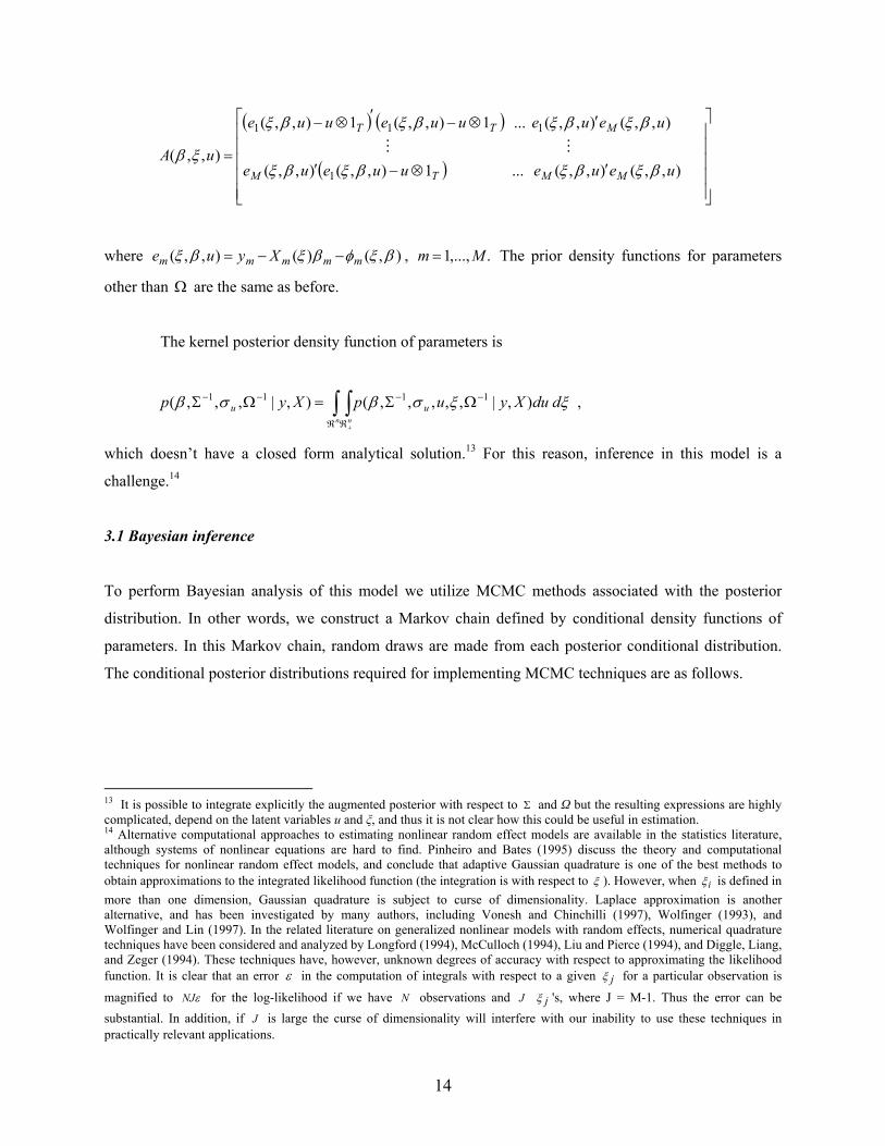
),,(),,( ... 1),,(),,(

),,(),,( ... 1),,(1),,(

),,(1

111

ueueuueue

ueueuueuue

uAMMTM

MTT

βξβξβξβξ

βξβξβξβξ

ξβ

where ),()(),,( βξφβξβξ mmmmm Xyue −−= , .,...,1 Mm = The prior density functions for parameters

other than Ω are the same as before.

The kernel posterior density function of parameters is

∫ ∫ℜ ℜ

−−−−

+

ΩΣ=ΩΣn n

dduXyupXyp uu ξξσβσβ ),|,,,,,(),|,,,( 1111 ,

which doesn’t have a closed form analytical solution.13 For this reason, inference in this model is a

challenge.14

3.1 Bayesian inference

To perform Bayesian analysis of this model we utilize MCMC methods associated with the posterior

distribution. In other words, we construct a Markov chain defined by conditional density functions of

parameters. In this Markov chain, random draws are made from each posterior conditional distribution.

The conditional posterior distributions required for implementing MCMC techniques are as follows.

13 It is possible to integrate explicitly the augmented posterior with respect to Σ and Ω but the resulting expressions are highly complicated, depend on the latent variables u and ξ, and thus it is not clear how this could be useful in estimation. 14 Alternative computational approaches to estimating nonlinear random effect models are available in the statistics literature, although systems of nonlinear equations are hard to find. Pinheiro and Bates (1995) discuss the theory and computational techniques for nonlinear random effect models, and conclude that adaptive Gaussian quadrature is one of the best methods to obtain approximations to the integrated likelihood function (the integration is with respect to ξ ). However, when is defined in more than one dimension, Gaussian quadrature is subject to curse of dimensionality. Laplace approximation is another alternative, and has been investigated by many authors, including Vonesh and Chinchilli (1997), Wolfinger (1993), and Wolfinger and Lin (1997). In the related literature on generalized nonlinear models with random effects, numerical quadrature techniques have been considered and analyzed by Longford (1994), McCulloch (1994), Liu and Pierce (1994), and Diggle, Liang, and Zeger (1994). These techniques have, however, unknown degrees of accuracy with respect to approximating the likelihood function. It is clear that an error

iξ

ε in the computation of integrals with respect to a given for a particular observation is

magnified to jξ

εNJ for the log-likelihood if we have observations and 's, where J = M-1. Thus the error can be substantial. In addition, if is large the curse of dimensionality will interfere with our inability to use these techniques in practically relevant applications.

N J jξ

J

14

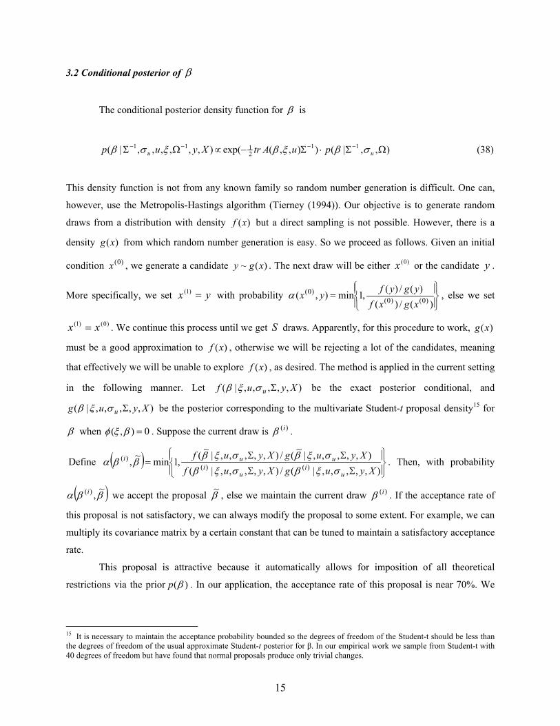
3.2 Conditional posterior of β

The conditional posterior density function for β is

),,|()),,(exp(),,,,,,|( 112111 ΩΣ⋅Σ−∝ΩΣ −−−−

uu puAtrXyup σβξβξσβ (38)

This density function is not from any known family so random number generation is difficult. One can,

however, use the Metropolis-Hastings algorithm (Tierney (1994)). Our objective is to generate random

draws from a distribution with density but a direct sampling is not possible. However, there is a

density from which random number generation is easy. So we proceed as follows. Given an initial

condition , we generate a candidate . The next draw will be either or the candidate .

More specifically, we set with probability

)(xf

~ gy

)(xg

0(x ) )(x )0(x y

yx =)1(

=)(

)( ,1min),( )0(0()0(

xxfyfyxα

), X

(/)(/)

) ggy , else we set

. We continue this process until we get draws. Apparently, for this procedure to work,

must be a good approximation to , otherwise we will be rejecting a lot of the candidates, meaning

that effectively we will be unable to explore , as desired. The method is applied in the current setting

in the following manner. Let

)0(x)1(x = S

,

)(xg

)(x

(f

f

)(x

,u

f

,,| u yΣσξβ be the exact posterior conditional, and

),, Xy,,,u u|(g Σσξβ be the posterior corresponding to the multivariate Student-t proposal density15 for

β when 0) =,( βξφ . Suppose the current draw is . )(β i

Define ( )

ΣΣ

ΣΣ=

),,,,,|(/),,,,,|(),,,,,|~(/),,,,,|~(,1min~, )()(

)(

XyugXyufXyugXyuf

ui

ui

uui

σξβσξβσξβσξβ

ββα . Then, with probability

( )β~ ββα ,)(i we accept the proposal ~ , else we maintain the current draw . If the acceptance rate of

this proposal is not satisfactory, we can always modify the proposal to some extent. For example, we can

multiply its covariance matrix by a certain constant that can be tuned to maintain a satisfactory acceptance

rate.

)(iβ

This proposal is attractive because it automatically allows for imposition of all theoretical

restrictions via the prior )(βp . In our application, the acceptance rate of this proposal is near 70%. We

15 It is necessary to maintain the acceptance probability bounded so the degrees of freedom of the Student-t should be less than the degrees of freedom of the usual approximate Student-t posterior for β. In our empirical work we sample from Student-t with 40 degrees of freedom but have found that normal proposals produce only trivial changes.

15

also impose the monotonicity and concavity restrictions at each sample point using the rejection method,

exactly as in the model with only technical inefficiency.

3.3 Conditional posterior of Σ

The posterior conditional density function of Σ is given by

))],,([exp(),,,,,,|( 1212

)1(111 −

Σ

+−+−−− Σ+−Σ∝ΩΣ

Σ

uAAtrXyupMn

u ξβξσβν

(39)

which is the density function of a Wishart distribution. Given u,,ξβ the matrix ),,( uA ξβ is a known

constant. So generating random draws from the above density function is straightforward.

3.4 Conditional posterior of Ω

The posterior conditional density function of Ω is

( )121

2/)(111 )]([exp),,,,,,|( −Ω

−+−−− Ω+−Ω∝ΣΩ Ω ξξσβν

QAtrXyupMn

u (40)

which is also the density function of a Wishart distribution since )(ξQA +Ω is a given matrix of

constants.

3.5 Conditional posterior of uσ

The posterior conditional density function of uσ satisfies

2112 ~,,,,,,| nnu

Xyuuuq

+−− ΩΣ

′+χξβ

σ (41)

from which random number generation is simple.

3.6 Conditional posterior of u

For latent technical inefficiency, it can easily be shown, using the techniques developed in the

previous section, that

16

niuNXyu iiui ...1 ,0 ),,(~,,,,,, 2*

*1

11 =≥ΩΣ −− σµξσβ (42)

where

∑=

==m

j

jjii niueT

1

12*

* ,...,1,),,( σβξσµ ; 211

22* 1 u

u

T σσσ

σ+

= ;

MmueueXyue mTmmmmmm ,...,1,]),,(),...,,,([),()(),,( 1 =′=−−= βξβξβξφβξβξ

),,(),,(1

1 ueTueT

tmtm βξβξ ∑

=

−= , Mm ,...,1= is a 1×n vector with

]),,(),...,,,([),,( 1 ′= eueue mnmm uβξβξβξ , M,...,m 1=

and the inverse contemporaneous covariance matrix is expressed as Σ . This distribution of is

truncated normal, and since the 's are independent in their joint posterior conditional distribution,

random draws can be generated sequentially for each i

][1 ijσ=−iu

iu

n,...,1= as in Tsionas (1999).

3.7 Conditional posterior of ξ

Finally, we consider the posterior conditional density function of ξ given by

( )1211

2111 )(exp)),,(exp(),,,,,,|( −−−− Ω−⋅Σ−∝ΩΣ ξξβσβξ trQuAtrXyup u (43)

Generating random draws from this joint density function is not straightforward because the density

function is not from any known form. One promising possibility to obtain a reasonably good proposal

density function is to linearize the cost share equations (i.e., to make them linear in theξ 's). The resulting

approximate posterior of each iξ will be normal so in practice we can use a Student-t proposal density

function16 to maintain the acceptance probability bound. We can easily obtain a random draw from this

posterior, and use a Metropolis rule to maintain the correct posterior. The normal approximation is, in

fact, very simple to use. The task is to linearize the cost function and share equations with respect to ξ

and use the approximation to obtain a multivariate normal or Student-t density function for the ξ 's that

can be used as proposal density function for the Metropolis-Hastings step. In Appendix A we show that

partial derivatives of the cost function with respect to ξ 's are exactly zero, so we can use only the share

equations to derive the linear approximation so the normal approximation has a particularly simple

16 We use a Student-t with 10 degrees of freedom but we have found the results remain the same when we use a normal proposal.

17

structure for the translog cost system. The acceptance rate of the Metropolis chain is over 85% for the

data we analyzed, which is a satisfactory approximation.17 Let iξ be the current draw from the

approximate density function. Let ),,,,|( ΩΣβξ Xyf i be the exact conditional density function of iξ

given the data and the parameters, and ),,,|( Ωβξ Xyg i

,|(~

be the normal approximation, i.e., the pdf of the

multivariate normal resulting from the normal approximation. Clearly, both density functions are

available in closed form. The candidate ),,, ΩΣβξξ Xyf ii

)

will either be accepted or rejected in

favor of the previous draw, say , according to the following rule. Let 0(iξ

ΩΣ

ΩΣ

(/),,,,||(/),,,,|0(ξβ

ξβgXygXy

i

i Ω

,,,|,,,β

βXy

Xy()0(ξξf

i

i)

( )iξ,)0

i(ξ

iξ

iξ

)D

( )

Ω=

)() ,1min,)0( ξξ

fa ii

Either we accept this draw with probability a , or reject it and take as the draw. The

overall acceptance rate of this procedure is over 85% in the data set we have analyzed. It is necessary to

ensure that the approximation to the exact conditional posterior of

)0(iξ

is satisfactory. We cannot claim

that this will always be the case but we suspect that when this is not so, the approximation can be

improved adaptively by linearizing around a point (different from zero) that could be the current

posterior mean of .iξ18

3.8 Joint measurement of technical and allocative inefficiency

The previous model is capable of providing measures of technical and allocative inefficiency for

each firm, and for a yet unobserved firm (in which case we make posterior predictive inferences, i.e.,

predictive inferences conditional on the observed data). Our problem here is as follows. Suppose ,(f θ

17 Following the sampling theory literature we could have used Gaussian quadrature to integrate out ξ's from the likelihood function or the posterior distribution, and then use the Metropolis-Hastings algorithm (MHA) to provide inferences for β, Σ, Ω. The required posterior would not, of course, be available in closed form. We did not opt for this technique because the MHA does not take account of the special features of the problem, namely linearity of the system conditional on ξ's. Moreover, for complicated posteriors, the MHA can result in high autocorrelation of the draws, making reliable exploration of the posterior a troublesome task. 18 We have tried this approximation in our application and found that the acceptance rate increased slightly. However, we decided not to use it in reporting the final results since the original proposal performed rather well. Another advantage of the algorithm is that it can be vectorized easily to generate all iξ 's at once by exploiting properties of the normal distribution. Consequently, fitting the nonlinear translog random effect model is not considerably more time consuming compared to the translog system with only technical inefficiency.

18

represents any function of the parameters θ (inclusive, perhaps, of any latent variables like and u ξ )

and the data D . The objective is to estimate the posterior expectation

Given draws , from the posterior density function

∫= θθ DpDfDEf )|),(),

)|( Dp

θd( .θ(

)(sθ Ss ,...,1= θ , this expectation can be

approximated by . [ ]DDf |),(θ ∑=

−≈S

s

s DfS1

)1 ),E ((θ

( y| )X

(iu

rE i ,

)s

)(sir

)(sir

i

s

uu σ| i

uir σ|

≈|() uuu ddatap σσ

ir

)(suσ Ss ,...,1=∫

∞

=0

|( irp σ

u

))( irp

σ

jξ ξ )(,sijξ

∑=

−S

sij S

1

1,ξ =

)1,j

)()( ss

Next, we describe the procedure to obtain technical and allocative inefficiency measures.

Measurement of technical inefficiency in the present model is exactly the same as in the model without

allocative inefficiency presented in section 2. Define )exp( ii ur −= to be the efficiency index of firm

. The firm-specific efficiency measure is provided by the mean of the posterior density function

of , viz., . This measure can be obtained by averaging , where denotes the th

draw for . Once a draw from the conditional posterior of u

ni ,...,1=

ir

ir i becomes available, this can be

computed easily. The posterior predictive density function can also be obtained easily. Since s

half normal, the density function of can be obtained easily. The marginal density function of is

then given by where , denotes the

posterior draws for

∑=1

)( )|(S

s

suirp σ−1S

.

Regarding allocative inefficiency we follow a similar procedure. First, the departure of observed

prices from shadow prices, namely the 's, are of interest. Given the posterior draws for , say , a

firm-specific measure is provided by sij)(

,ξ where indicates the number of draws. This

gives the percentage deviation of observed prices from shadow prices for input pair ( for firm i . The

deviations themselves can be estimated from

S

∑=

Ssij

1

)(,λ−=

sij S 1

,λ , where , . ),i sexp(, jij ξλ = S,...,1=

Another measure of interest is the percentage increase in costs due to allocative inefficiency for

each firm. This is given by and depends on the data, the ALitCln ξ s and the parameters in β . Clearly,

this measure can be computed for each draw of β and ξ . It can be averaged with respect to the draws,

and provide temporal and firm-specific measures for or . A posterior predictive density

function for , referring to an as of yet unobserved (or a typical) firm is computed as follows. Given

a vector of prices and output for that firm (for example, the sample averages of these variables) is

ALitCln AL

itC

ALCln

ALCln

19

computed for each draw, and then averaged with respect to the draws. This provides information

regarding the distribution of allocative inefficiency for a typical firm conditional on the data, and can be

used for predictive purposes. Parameter uncertainty is fully taken into account in these computations in

standard Bayesian fashion since these measures are averaged against the posterior distribution of

parameters. The implication, of course, is that we do not have to resort to asymptotic approximations of

the "plug-in" variety. Similar principles are followed to compute the firm-specific measures for . ALCln

TEjj x=

== uaC

Further information can be obtained from Bayesian inferences regarding whether certain inputs

are under- or over- utilized. This information is not provided by the ξ 's alone. Since ∂ and

where and denote technically efficient and optimal (both technically and

allocatively efficient) quantities of input x

wC ∂/*

OPjj xwC =∂∂ /0 TE

jx OPjx

j (with firm and time subscripts omitted) and 0*C ,

non-optimal use of input xj relative to input x1 (for example), can be obtained from the formula19

( ) ( ) .,...,2for/1//1)exp()//()/( 0

110

11 mjSSxxxx jjjOP

jTE

jj =++−== ηηξκ

Consequently, if )(<>jκ 1 then input xj is over- (under-) used relative to input x1. Note that these

measures are firm-specific and time-varying. Using the MCMC algorithm we have one draw for each of

the jκ . This draw depends on all parameters of the system. The final measure is obtained by averaging

across all draws using the standard estimator. This operation is equivalent to integrating parameter

uncertainty out.

It is clear that the model developed in this section provides all the information that we need to

evaluate technical and allocative inefficiency for each firm in the sample using a cost system (consisting

of the cost function and cost share equations). There are four basic advantages of the model we proposed

in this section. First, technical and allocative inefficiency are modeled in a way that is consistent with the

cost minimization problem of standard microeconomic theory. Second, all inferences are for the given

data, so no asymptotic approximations are used. Third, using a systems approach ensures that we obtain

more precise estimates of technical efficiency relative to a single equation approach. Finally, it solves the

Greene problem from an empirical point of view.20

19 Alternatively, one can define non-optimal use of input xj from OP

jTEjj xx /=κ

( ) .,...,1for)exp()(/1)exp( 00 mjSS kkk

kjjj =−++−= ∑ ηηηξ Thus, if 1)(<>jκ then input xj is over-used (under-used).

20 An anonymous referee mentioned that a fixed effects model would also have these advantages. While this is true, we argue that there are situations (for example, cross-sectional models) where one cannot use a fixed effects model. Furthermore, in a fixed effects model technical inefficiency is defined relative to the best firm in the sample. This is, however, not the case in the present model.

20

4. Prior specifications

In our empirical application we use two priors (A and B). Both priors have 1=n . Prior A has

1.0=q and prior B has 1=q . Prior median efficiency is 71% and 41.8% respectively. We choose 1=n

because n represents the number of observations in a fictitious experiment that provides a random

sample nuu ,...1 with variance nq / . Therefore, prior information exists but is not particularly precise.

For the semi-informative prior to accommodate the restrictions implied by economic theory we

assume where . This prior is extremely tight and practically implies exact

imposition of the restrictions. The exact form of the restrictions for this application is presented in

Appendix B. Since these are mathematical restrictions to be satisfied by any cost function, we decided to

impose these constraints exactly. Nonetheless, we argue that the proposed method allows one to use

different degrees of correctness. We use informative priors for both

),0(~ 2qq ING εβ 510−=ε

Σ and Ω which are both inverted

Wishart with 1== ΩΣ νν degree of freedom and scale matrix . These priors are proper

but very diffuse.

I5−AA 10Σ == Ω

5. Data and empirical results

5.1 Data

The data for this study is taken from the commercial bank and bank holding company database

managed by the Federal Reserve Bank of Chicago. It is based on the Report of Condition and Income

(Call Report) for all U.S. commercial banks that report to the Federal Reserve banks and the FDIC. In this

paper we used the data for the years 1996-2000 and selected a random sample of 500 commercial banks.

The commercial banking industry is one of the largest and most important sectors of the US

economy. The structure of the banking industry has undergone rapid changes in the last two decades,

mostly due to extensive consolidation. Justification of mergers and acquisitions is often provided in terms

of economies of scale and efficiency. Here we focus on the efficiency arguments by estimating a flexible

cost system. Previous banking efficiency studies (see the survey by Berger and Humphrey (1997)) based

on cost function estimation mostly focused on technical inefficiency. The reason for this is that estimation

of the translog system with both technical and allocative inefficiency was not feasible before. From this

perspective, this is the first banking study in which a translog cost function system with technical and

21

allocative inefficiency are jointly estimated without making them deterministic functions of data and

unknown parameters.

In the banking literature there is controversy regarding the choice of inputs and outputs. Here we

follow the intermediation approach (Kaparakis et al. (1994) in which banks are viewed as financial firms

transforming various financial and physical resources into loans and investments. The output variables

are: installment loans (to individuals for personal/household expenses) (y1), real estate loans (y2),

business loans (y3), federal funds sold and securities purchased under agreements to resell (y4), other

assets (assets that cannot be properly included in any other asset items in the balance sheet) (y5). The

input variables are: labor (x1), capital (x2), purchased funds (x3), interest-bearing deposits in total

transaction accounts (x4) and interest-bearing deposits in total nontransaction accounts (x5). For each

input the price is obtained by dividing total expenses on it by the corresponding input quantity. Thus, for

example, the price of labor (w1) is obtained from expenses on salaries and benefits divided by the number

of full time employees (x1). The same approach is used to obtain w2 through w5. Total cost is then defined

as the sum of the expenses on these five inputs. To impose the linear homogeneity restrictions, we

normalize total cost and all the prices with respect to . 5w

5.2 Empirical results

5.2.1 Technical efficiency

The model for technical efficiency only with a single output is outlined in equation (1). Here we

write it out fully for five outputs and five inputs using the translog functional form

iititjj

jtitmm

mttttj

itmitjm

jm

j j kitkitjjkitqitm

m qmqitm

mmitjj

ait

uvtwtyttyw

wwyyywC

+++++++

++++=

∑∑∑∑

∑ ∑∑∑∑

,1,,2

21

,,

,,21

,,21

,,0

lnlnlnln

lnlnlnlnlnlnln

ββααγ

βγγαα ∑

and

4,...,1,;5,...,1,,lnln ,1,,, ==++++= +∑ ∑ kjqmvtywS itjjtitmk m

jmitkjkja

itj βγβα .

The assumptions on the noise components (v1,…,v5), and technical inefficiency component, u are as

before and are not repeated here.

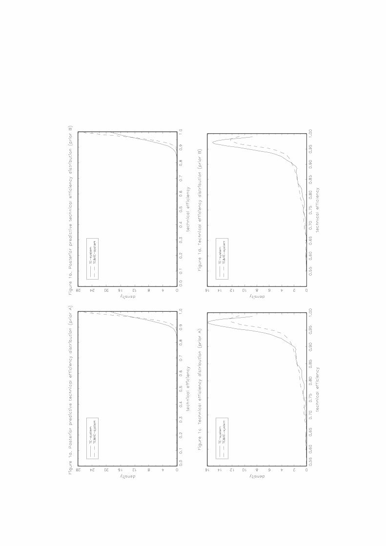
In Figure 1 we provide the posterior predictive technical efficiency as well as kernel density

estimates for firm-specific technical efficiency measures for both priors A and B. We considered two

models: (i) the translog cost system with only technical inefficiency, and (ii) the translog cost system with

22

both technical and allocative inefficiency. In Figures 1a and 1b we provide the posterior predictive

technical efficiency distributions, which give the density function of technical efficiency for a typical or

yet unobserved firm. The results from the two systems (with and without allocative inefficiency) are quite

similar. This doesn’t mean that allocative inefficiency can be ignored.21 Since the overall cost efficiency

is the product of technical and allocative efficiency, i.e., OE AETE ⋅= (Farrell (1957)), and both TE

and AE are less than unity – the estimated TE in the technical inefficiency only model (where OE = TE

by construction) is likely to be biased upward. In Figures 1c and 1d we report kernel densities of firm-

specific efficiency measures. For each bank in the sample, its technical efficiency measure is the mean of

the distribution of technical efficiency of that bank, conditional on its data, and unconditional on the

parameters. In other words, parameter uncertainty is accounted for in estimating technical efficiency.

Figures 1c and 1d present the kernel densities of these bank-specific efficiency means. Results from both

models show that efficiency values below 70% are highly improbable.22

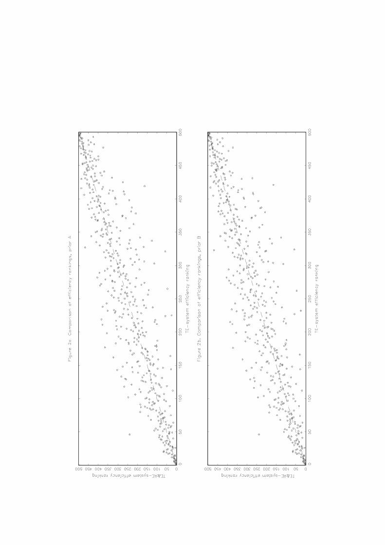
In Figure 2 we report efficiency rankings (technical) of banks from models with only technical

inefficiency and with both technical and allocative inefficiency. Generally, the correlations between these

rankings are fairly high but for some specific banks large differences are observed. Thus, if the focus is

individual bank efficiency the high correlation of efficiency ranking between models may not be useful in

choosing between models.

5.2.2. Allocative efficiency

We now discuss results obtained from the system with both technical and allocative inefficiency.

The density functions of allocative inefficiency (price distortion) ( jξ ) are reported in Figure 3a and 3b,

and some summary measures are reported in Table 1. Each graph23 provides the kernel density estimate of

bank-specific average of jξ . It may be useful to describe again how these density functions arise. For the

th bank in the sample the Gibbs sampler provides a random draw during iteration for

input pair Recall that this is a draw from the distribution of

i )()(s

jiξ

ji)

Ss ,...,1=

).1,( j (ξ conditional on the data and all

21 Note that ignoring allocative inefficiency, if any, makes the model misspecified that results wrong parameter estimates since the allocative inefficiency component in a translog cost function depends on outputs and input prices in a non-linear fashion. 22 We examine convergence of our MCMC sampling schemes using Geweke's convergence diagnostics, as well as by running multiple chains starting from over-dispersed initial conditions and checking whether final marginal posteriors are close. Models with or without allocative inefficiency seemed very robust to initial conditions and passed convergence tests. Additionally, we have examined autocorrelation functions of posterior draws. To reduce the autocorrelation, we use the batching technique that is standard in the simulation literature. Batch means display practically zero autocorrelations. Results in graphical form are available upon request. 23 We do not report posterior predictive distributions for allocative inefficiency measures since we are interested mostly in inferences regarding the banks in our sample.

23

other parameters of the model. What we need is the density function of ji)(ξ conditional on the data only.

To average out parameter uncertainty we compute ∑=

−=S

s

sjiji S

1

)()(

1)( ξξ which provides a price distortion

measure for each input and each bank. Figure 4 presents kernel densities of ji)(ξ across banks for any

given input . These density functions do not vary widely with the prior of the technical

efficiency parameter

4,...,1=j

uσ . They are concentrated around zero (so we can claim that, banks on average do

not seem to have significant relative price distortions) but they differ in terms of spread and overall shape.

For labor (input 1), relative price distortions can be as large as 8% in absolute value. For other inputs, the

spread is much lower and distortions range from minus 4% to plus 4%. The difference in spreads reflects

the fact that for labor (relative to input 5) banks seem to misperceive prices to a greater extent compared

to other inputs. Finally, the fact that these density functions are not particularly tight means that banks are

quite heterogeneous in terms of allocative inefficiency.

1κ

Cln

The density functions of jκ (relative over- (under-) use of each input) are reported in Figures 3c

and 3d, and their summary measures are reported in Table 1. These density functions are kernel density

estimates of bank-specific measures derived following the formula given in the previous paragraph. These

density functions are mostly centered around unity meaning that, on average, banks do not make many

allocative mistakes in using their inputs. The considerable spread suggests that banks are highly

heterogeneous in their relative input mis-allocation. More specifically, ranges from 0.836 to 1.182

suggesting that banks may under-utilize labor (relative to input 5) by as much as 17.4% or over-utilize it

by as much as 18.2%. The remaining jκ ranges roughly from 0.92 to 1.08 suggesting under-utilization

by 8% and over-utilization by 8%. Thus we observe the presence of considerable allocative inefficiency

in the sample banks.

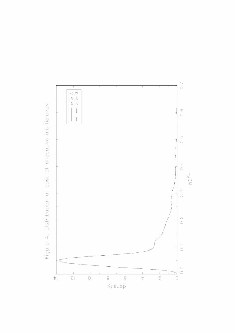
When banks fail to allocate their inputs properly, costs will increase. We label this as the cost of

allocative inefficiency. In Figure 4 we provide kernel densities of bank-specific measures of percentage

increases in cost due to allocative inefficiency, . The density functions of are highly skewed

to the right. On average, allocative inefficiency increased cost by 10% (meaning that on average, cost

allocative efficiency is 90%), although there are fewer banks for which this is much higher. From the

practical point of view optimal use of inputs is driven by the motive of attaining high cost efficiency.

Since some inputs are costlier than others a relatively cheap (expensive) input can be over- (under-) used

more than some other inputs that are relatively costly. Here we show how to obtain information on

allocative inefficiency (defined in terms of price distortion), non-optimal input use and finally the cost of

non-optimal input use, along with cost of technical inefficiency.

ALCln AL

24

We have tried several prior tightness parameters for the regression parameters, β , viz.,ε ranging

from to 0.1 without noticing large differences in final results related to technical and allocative

inefficiency. We have also tried larger values for the prior tightness parameter. In these cases the results

started to differ notably. This type of outcome is quite reasonable. With small values of the prior tightness

we can interpret the model as a cost-share system, at least in an approximate sense. We necessarily lose

this interpretation as the value of prior tightness increases. In this case the interpretation of technical

efficiency becomes ambiguous so it should be expected that the results become more sensitive on the

prior.

1210−

6. Conclusions

In this paper we developed Bayesian tools for making inferences on firm-specific technical and

allocative inefficiency using a system approach. The system considered here is based on the cost

minimization behavior of producers. The main contribution of the paper is the estimation of a well-

specified translog system (in which the error terms in the cost and cost-share equations are internally

consistent) in a random effects framework. This solves the Greene problem by using a model that is

theoretically consistent and estimating it without treating the inefficiencies as parametric functions of the

data and unknown parameters. First, we analyzed the model with only technical inefficiency and then we

introduced allocative inefficiency. The model with only technical inefficiency is a standard seemingly

unrelated regressions system conditional on the latent inefficiency variable. The model with both

technical and allocative inefficiency is a nonlinear seemingly unrelated regression with nonlinear random

effects. We showed that simulation-based numerical Bayesian analysis can be used to provide inferences

on parameters and more importantly on functions of interest, viz., technical efficiency, allocative

inefficiency, price distortions for each input, non-optimal input use for each input, etc., for each firm. The

new techniques are applied to a panel of U.S. banks. We compared the results obtained from two system

approaches, namely with and without allocative inefficiency. Results show some important differences in

efficiency estimates across models.

References

Aigner, D.J., C.A.K. Lovell, and P. Schmidt, 1977, Formulation and estimation of stochastic frontier

production function models, Journal of Econometrics 6, 21-37. Atkinson, S. E., and C. Cornwell, 1994, Parametric estimation of technical and allocative inefficiency

with panel data, International Economic Review 35, 231-244. Bauer, P.W., 1990, Recent developments in the econometric estimation of frontiers, Journal of

Econometrics 46, 39-56.

25

Berger, A. N. and D. B. Humphrey, 1997, Efficiency of financial institutions: International survey and directions for future research, European Journal of Operational Research 98, 175-212.

van den Broeck, J., G. Koop, J. Osiewalski, and M.F.J. Steel, 1994, Stochastic frontier models: A Bayesian perspective, Journal of Econometrics 61, 273-303.

Casella, G. and E. George, 1992, Explaining the Gibbs sampler, The American Statistician 46, 167-174. Chen, L., Z. Qin, and J.S. Liu, 2000, Exploring hybrid Monte Carlo in Bayesian computation, in: E.I.

George, ed., Bayesian Methods with Applications to Science, Policy, and Official Statistics, Selected Papers from ISBA 2000: The Sixth World Meeting of the International Society for Bayesian Analysis, 71-80.

Christensen, L. R., and W.H. Greene, 1976, Economies of scale in U. S. electric power generation, Journal of Political Economy 84, 655-76.

Diewert, W.E., and T.J. Wales, 1987, Flexible functional forms and global curvature conditions, Econometrica 55, 43-68.

Diewert, W.E., 1982, Duality approaches to microeconomic theory, in: K.J. Arrow and M.D. Intriligator, eds., Handbook of Mathematical Economics, Vol II (North-Holland, Amsterdam).

Diggle, P.J., K.Y. Liang, and S.L. Zeger, 1994, Analysis of longitudinal data (Clarendon Press, Oxford). Farrell, M. J., 1957, The measurement of productive efficiency, Journal of the Royal Statistical Society,

Series A, 120, 253-81. Fernandez, C., G. Koop, and M.F.J. Steel, 2000, A Bayesian analysis of multiple output stochastic

frontiers, Journal of Econometrics 98, 47-79. Fernandez, C., J. Osiewalski, and M.F.J. Steel, 1997, On the use of panel data in stochastic frontier

models. Journal of Econometrics 79, 169-193 Gelfand, A..E. and A.F.M. Smith, 1990, Sampling based approaches to calculating marginal densities,

Journal of the American Statistical Association 85, 398-409. Geweke, J., 1993, Bayesian treatment of the independent Student-t linear model, Journal of Applied

Econometrics 8, S19-S40. Geweke, J., 1999, Using simulation methods for Bayesian econometric models: Inference, development

and communication (with discussion and rejoinder), Econometric Reviews 18, 1-126. Greene, W.H., 1980, On the estimation of a flexible frontier production model, Journal of Econometrics

13:1, 101-15. Greene, W.H., 1993, The econometric approach to efficiency analysis, in: H.O. Fried, C.A.K. Lovell and

S.S. Schmidt, eds., The measurement of productive efficiency: Techniques and applications (Oxford University Press, Oxford) 68-119.

Greene, W.H., 2001, New developments in the estimation of stochastic frontier models with panel data, (Department of Economics, Stern School of Business, New York University, NY).

Griffiths, W.E., 2001, Bayesian inference in the seemingly unrelated regressions models, in D. Giles, ed., Computer-Aided Econometrics, Marcel Dekker (forthcoming).

Kalirajan, K. P., 1990, On Measuring Economic Efficiency, Journal of Applied Econometrics 5, 75-85. Kaparakis, E.I., S.M. Miller, and A. Noulas, 1994, Short-run cost-inefficiency of commercial banks: A

flexible stochastic frontier approach, Journal of Money, Credit and Banking 26, 875-893. Koop, G, J. Osiewalski, and M.F.J. Steel, 1997, Bayesian efficiency analysis through individual effects:

Hospital cost frontiers, Journal of Econometrics 76: 77-105. Koop, G. and M.F.J. Steel, 2001, Bayesian analysis of stochastic frontier models, in: Baltagi B., ed., A

Companion to Theoretical Econometrics (Blackwell, Oxford) 520-573. Koop, G., M.F.J. Steel, and J. Osiewalski, 1995, Posterior analysis of stochastic frontier models using

Gibbs sampling, Computational Statistics 10, 353-373. Kumbhakar, S.C., 1987, The specification of technical and allocative inefficiency in stochastic production

and profit frontiers, Journal of Econometrics 34, 335-48. Kumbhakar, S.C., 1997, Modeling allocative inefficiency in a translog cost function and cost share

equations: An exact relationship, Journal of Econometrics 76, 351-356.

26

Kumbhakar, S.C. and C.A.K Lovell, 2000, Stochastic frontier analysis (Cambridge University Press, New York).

Liu, Q. and D.A. Pierce, 1994, A note on Gauss-Hermite quadrature, Biometrika 81, 624-629. Longford, N.T., 1994, Logistic regression with random coefficients, Computational Statistics and Data

Analysis 17, 1-15. Maietta, O.W., 2002, The decomposition of cost efficiency into technical and allocative efficiency with

panel data of Italian dairy farms, European Review of Agricultural Economics, 27, 473-495. McCulloch, C.E., 1994, Maximum likelihood variance components estimation for binary data, Journal of

the American Statistical Association 89, 330-335. Meeusen, W., J. van den Broeck, 1977, Efficiency estimation from Cobb-Douglas production functions

with composed error, International Economic Review 8, 435-444. Pinheiro, J.C. and D.M. Bates, 1995, Approximations to the log-likelihood function in the nonlinear

mixed-effects model, Journal of Computational and Graphical Statistics 4, 12-35. Roberts, G.O. and A.F.M. Smith, 1994, Simple conditions for the convergence of the Gibbs sampler and

Metropolis-Hastings algorithms, Stochastic Processes and their Applications 49, 207-216. Schmidt, P., and C.A.K. Lovell, 1979, Estimating technical and allocative inefficiency relative to

stochastic production and cost frontiers, Journal of Econometrics 9, 343-66. Tanner, M.A. and W.H. Wong, 1987, The calculation of posterior distributions by data augmentation.

Journal of the American Statistical Association 82, 528-550. Tierney, L., 1994, Markov chains for exploring posterior distributions (with discussion), Annals of

Statistics 22, 1701-1762. Tsionas, E.G., 1999, Full likelihood inference in normal-gamma stochastic frontier models, Journal of

Productivity Analysis 13, 179-201. Vonesh, E.F. and V.M. Chinchilli, 1997, Linear and nonlinear models for the analysis of repeated

measurements (Marcel Dekker, New York). Wolfinger, R.D., 1993, Laplace's approximation for nonlinear mixed models, Biometrika 80, 791-795. Wolfinger, R.D. and X. Lin, 1997, Two Taylor-series approximation methods for nonlinear mixed

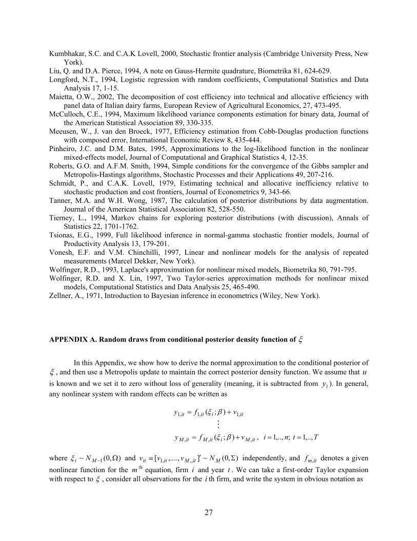
models, Computational Statistics and Data Analysis 25, 465-490. Zellner, A., 1971, Introduction to Bayesian inference in econometrics (Wiley, New York). APPENDIX A. Random draws from conditional posterior density function of ξ

In this Appendix, we show how to derive the normal approximation to the conditional posterior of

ξ , and then use a Metropolis update to maintain the correct posterior density function. We assume that u is known and we set it to zero without loss of generality (meaning, it is subtracted from ). In general, any nonlinear system with random effects can be written as

1y

itiitit vfy ,1,1,1 );( += βξ

itMiitMitM vfy ,,, );( += βξ , ;,..,1 ni = Tt ,..,1=

where ),0(~ 1 Ω−Mi Nξ and ),0(~],....,[ ,,,1 Σ′≡ MitMitit Nvvv

i independently, and denotes a given

nonlinear function for the itmf ,

m th equation, firm and year t . We can take a first-order Taylor expansion with respect to ξ , consider all observations for the th firm, and write the system in obvious notation as i

27

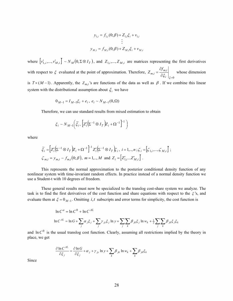
iiiii vZfy ,1,1,1,1 );0( ++= ξβ

iMiiMiMiM vZfy ,,,, );0( ++= ξβ where , and Z are matrices representing the first derivatives

with respect to

[ ] ( )TMiMi INvv ⊗Σ′′′ ,0~,..., ,,.1 iMi Z ,,1 ,...,

ξ evaluated at the point of approximation. Therefore, 0

,,

=∂

∂=

ξξ i

imim

fZ whose dimension

is . Apparently, the 's are functions of the data as well as )1( −M imZ ,×T β . If we combine this linear system with the distributional assumption about iξ we have

iiMM eI += −− ξ110 , ),0(~ 1 Ω−Mi Ne

Therefore, we can use standard results from mixed estimation to obtain

( )[ ]

Ω+⊗Σ′

−−−−

1111 ,~~ iTiiMi ZIZN ξξ

where

( )[ ] ( ) iTiiTii IZZIZ ζξ ⊗Σ′Ω+⊗Σ′= −−−− 1111~ , ni ,..,1= ; [ ]′= iMii ,,1 ,...,ζζζ ;

( )βζ ;0,,, imimim fy −= , and Mm ,..,1= [ ]′′′= iMii ZZZ ,,1 ... .

This represents the normal approximation to the posterior conditional density function of any nonlinear system with time-invariant random effects. In practice instead of a normal density function we use a Student-t with 10 degrees of freedom.

These general results must now be specialized to the translog cost-share system we analyze. The task is to find the first derivatives of the cost function and share equations with respect to the ξ 's, and evaluate them at 10 −= Mξ . Omitting subscripts and error terms for simplicity, the cost function is ti,

ALa CCC lnlnln 0 +=

∑∑∑ ∑ ∑∑ ++++=j k

kjjkj j j k

kjjkjjyjjAL wyGC ξξβξβξγξα 2

1lnlnlnln

and is the usual translog cost function. Clearly, assuming all restrictions implied by the theory in place, we get

0ln C

∑ ∑++++∂∂

=∂

∂

k kkjkkjkjyj

jj

ALwyGC ξββγα

ξξlnlnlnln

Since

28

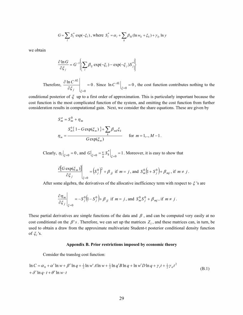
)exp(*∑ −=l

llSG ξ , where ∑ +++=k

lykklkll ywS ln)(ln* γξβα

we obtain

−−−=∂∂ ∑− *1 )exp()exp(ln

jjl

lljj

SGG ξξβξ

Therefore, 0ln

0

=∂

∂

=ξξ j

ALC . Since 00=

=ξALCln , the cost function contributes nothing to the

conditional posterior of ξ up to a first order of approximation. This is particularly important because the cost function is the most complicated function of the system, and omitting the cost function from further consideration results in computational gain. Next, we consider the share equations. These are given by

mmam SS η+= 0

)exp(

)exp(1 0

m

kkmkmm

m G

GS

ξ

ξβξη

∑+−= for 1,..,1 −= Mm .

Clearly, 00 ==ξηl , and ∑== ==

kkS 1

0*

0 ξξG . Moreover, it is easy to show that

[ ] ( ) jjj

j

m SG

βξξ

ξ

+=∂

∂

=

20

0

)exp( if jm = , and ( ) mjjm SS β++ 00 1 , if . jm ≠

After some algebra, the derivatives of the allocative inefficiency term with respect to ξ 's are

( ) jjjjj

m SS βξη

ξ

+−−=∂∂

=

00

0

1 if jm = , and , if mjjm SS β+00 jm ≠ .

These partial derivatives are simple functions of the data and β , and can be computed very easily at no cost conditional on the s'β . Therefore, we can set up the matrices , and these matrices can, in turn, be used to obtain a draw from the approximate multivariate Student-t posterior conditional density function of

iZ

iξ 's.

Appendix B. Prior restrictions imposed by economic theory

Consider the translog cost function:

twtqttqDwqBqwAwqwC ttt

⋅′+⋅′+

++′+′++′+′+=

lnlnlnlnlnlnln'lnlnlnln 2

21

21

21

0

θδγγβαα

(B.1)

29

where is the vector of log prices, ln is the wln 1×m q 1×s vector of log outputs, 0α is a constant, θα , and δβ , are and vectors, and A, B, D are matrices of dimensions , 1×m 1×s nm× ss× and

respectively. The share equations will be in the form sm×

tqGwFmS λ+++= lnln (B.2) where is the vector of input shares, F, G are matrices of dimensions m and S 1×m m× sm× respectively, and λ is an vector. 1×m

We impose exactly the restrictions that A and B are symmetric. Homogeneity implies

01' =Am , 1 1 ,0' =DS 1' =αm where 1 denotes the unit vector. Moreover, we have the cross-equation restrictions m 1×m

α=m , F = a, G = D, λθ =

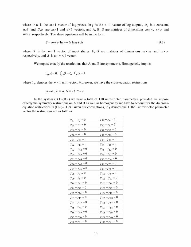
In the system (B.1)-(B.2) we have a total of 110 unrestricted parameters; provided we impose exactly the symmetry restrictions on A and B as well as homogeneity we have to account for the 44 cross-equation restrictions in (D.6)-(D.9). Given our conventions, if γ denotes the 110 1× unrestricted parameter vector the restrictions are as follows:

0267 =−γγ 0489 =−γγ

0768 =−γγ 0990 =−γγ

0869 =−γγ 01391 =−γγ

0970 =−γγ 01692 =−γγ

01071 =−γγ 01793 =−γγ

01172 =−γγ 01894 =−γγ

04273 =−γγ 05295 =−γγ

04374 =−γγ 05396 =−γγ

04475 =−γγ 05497 =−γγ

04576 =−γγ 05598 =−γγ

04677 =−γγ 05699 =−γγ

0378 =−γγ 05100 =−γγ

0879 =−γγ 010101 =−γγ

01280 =−γγ 014102 =−γγ

01381 =−γγ 017103 =−γγ

01482 =−γγ 019104 =−γγ

01583 =−γγ 020105 =−γγ

04784 =−γγ 057106 =−γγ

04885 =−γγ 058107 =−γγ

04986 =−γγ 059108 =−γγ

05087 =−γγ 060109 =−γγ

05188 =−γγ 061110 =−γγ

30

31

Since all restrictions are linear, they can be put in the form gG =γ where is , and G 11044× g

is . Based on this formulation a semi-informative prior can be specified in the form 144×~ 44N ),( HgGγ where H is 44 . 44×

Table 1. Posterior results for functions of interest*

Prior A Prior B Posterior predictive technical efficiency

0.963 (0.032)

0.963 (0.035)

Firm-specific technical efficiency

0.868 (0.247)

0.859 (0.257)

ALCln 0.099 (0.088)

0.098 (0.088)

1ξ -0.0016 (0.033)

-0.0016 (0.033)

2ξ -0.0056 (0.011)

-0.0055 (0.011)

3ξ 0.0029 (0.024)

0.0028 (0.024)

4ξ 0.0011 (0.008)

0.0009 (0.008)

1κ 1.0038 (0.059)

1.0038 (0.058)

2κ 1.017 (0.026)

1.017 (0.027)

3κ 0.991 (0.035)

0.991 (0.034)

4κ 0.996 (0.025)

0.996 (0.025)

* The entries are the posterior means. Posterior standard deviations appear in parentheses.