0
Connections between the Mass Balance, Ice Dynamics and Hypsometry
of White Glacier, Axel Heiberg Island, Nunavut
Laura Irene Thomson
A thesis submitted to the
Faculty of Graduate and Postdoctoral Studies
in partial fulfillment of the requirements
for the Doctorate in Philosophy in Geography
Department of Geography, Environment and Geomatics
Faculty of Arts
University of Ottawa
© Laura Thomson, Ottawa, Canada, 2016

ii
ABSTRACT
This thesis investigates how changing climate conditions have impacted the mass balance,
dynamics and associated hypsometry (area-elevation distribution) of White Glacier, an alpine
glacier on Axel Heiberg Island, Nunavut.
The first article describes the production of a new map of White Glacier from which
changes in ice thickness and glacier hypsometry could be determined. A new digital elevation
model (DEM) was created using >400 oblique air photos and Structure from Motion, a method
built upon photogrammetry but with the advantage of automated image correlation analysis. The
result of this work demonstrates that the method is able to overcome the challenges of optical
remote sensing in snow-covered areas. The resulting DEM and orthoimage facilitated the
production of a map with 5 m vertical accuracy in the style of earlier cartographic works.
The new map supported the calculation of the glacier’s geodetic mass balance and provides
an updated glacier hypsometry, which improves the accuracy of mass balance calculations. A
modeled glacier hypsometry time-series was created to support a reanalysis of the mass balance
record over the period 1960-2014, which through comparison of the geodetic and glaciological
methods enables the detection of potential sources of error in the glaciological method.
Comparison of the two approaches reveals that within the error margin no significant difference
exists between the average annual glaciological mass balance (-213 ± 28 mm w.e. a-1) and geodetic
mass balance (-178 ± 16 mm w.e. a-1).
To determine how ice dynamics have responded to ice thinning and negative mass
balances, dual-frequency GPS observations of ice motion were compared to historic velocity
measurements collected at three cross-sectional profiles along the glacier. Comparisons of annual
and seasonal velocities indicate velocity decreases of 10–45% since the 1960s. However, increased
summer velocities at the highest station suggests that increased delivery of surface meltwater to
the glacier bed has initiated basal sliding at elevations that did not experience high levels of melt
in earlier decades. Modeled balance fluxes demonstrate that observed fluxes, both historically and
currently, are unsustainable under current climate conditions.

iii
I don't know anything,
but I do know that everything is interesting
if you go into it deeply enough.
- Dr. Richard Feynman (1918-1988)

iv
TABLE OF CONTENTS
ABSTRACT ................................................................................................................................... ii
LIST OF FIGURES ..................................................................................................................... vi
LIST OF TABLES ...................................................................................................................... vii
ACKNOWLEDGEMENTS ...................................................................................................... viii
CHAPTER 1: INTRODUCTION ................................................................................................ 1
1.1 BACKGROUND AND MOTIVATION .............................................................................. 1
1.2 FOCUS AND OBJECTIVES ............................................................................................... 4
1.3 STUDY LOCATION AND REGIONAL CLIMATE .......................................................... 5
1.4 THESIS FORMAT ............................................................................................................... 7
CHAPTER 2: GLACIER MAPPING USING STRUCTURE FROM MOTION ................ 11
2.1 ARTICLE 1 SUMMARY AND ATTESTATION ............................................................. 11
2.2 INTRODUCTION .............................................................................................................. 11
2.3 METHODS 2.3.1 AERIAL PHOTOGRAPH SURVEY AND IMAGE POST-
PROCESSING .......................................................................................................................... 13
2.3.2 Model Building.......................................................................................................... 14
2.3.3 Ground Control and Marker Errors ......................................................................... 15
2.3.4 Model Results ............................................................................................................ 16
2.4 MAP CONSTRUCTION AND DESIGN ........................................................................... 17
2.4.1 Coordinate system and layout ................................................................................... 17
2.4.2 Contours .................................................................................................................... 17 2.4.3 Relief Shading ........................................................................................................... 18 2.4.4 Glacial and proglacial features ................................................................................ 18
2.4.5 Survey cairns, spot elevations, and reference prisms ............................................... 19 2.4.6 Map accuracy............................................................................................................ 19
2.5 CONCLUSIONS................................................................................................................. 21
CHAPTER 3: MASS BALANCE REANALYSIS ................................................................... 30
3.1 ARTICLE 2 SUMMARY AND ATTESTATION ............................................................. 30
3.2 INTRODUCTION .............................................................................................................. 31
3.3 STUDY SITE AND PREVIOUS RESEARCH .................................................................. 33
3.4 METHODS AND DATA ................................................................................................... 34
3.4.1 Glaciological Balance Measurements and Calculation ........................................... 34 3.4.2 Conventional Balances ............................................................................................. 36 3.4.3 Geodetic Balance ...................................................................................................... 37 3.4.4 DEM Coregistration ................................................................................................. 38
v
3.5 RANDOM AND SYSTEMATIC ERRORS ...................................................................... 39
3.6 CORRECTIONS OF GENERIC DIFFERENCES ............................................................. 40
3.6.1 Density Conversion ................................................................................................... 40 3.6.2 Survey Differences .................................................................................................... 40
3.6.3 Internal and Basal Mass Balance ............................................................................. 41
3.7 RESULTS AND DISCUSSION ......................................................................................... 43
3.8 CONCLUSIONS................................................................................................................. 47
CHAPTER 4: OBSERVATIONS OF MULTI-DECADAL VELOCITY FLUCTUATIONS
AND MECHANISMS DRIVING LONG-TERM SLOWDOWN .......................................... 57
4.1. ARTICLE 3 SUMMARY AND ATTESTATION ............................................................ 57
4.2 INTRODUCTION .............................................................................................................. 57
4.3 STUDY LOCATION .......................................................................................................... 60
4.4 METHODS ......................................................................................................................... 61
4.4.1 Velocity observations 1960-1970 .............................................................................. 61 4.4.2 Velocity observations 2012-2016 .............................................................................. 62
4.4.3 Surface elevations ..................................................................................................... 63 4.4.4 Ice thickness .............................................................................................................. 63
4.5 RESULTS ........................................................................................................................... 64
4.6 DISCUSSION ..................................................................................................................... 65
4.6.1 Internal deformation ................................................................................................. 66 4.6.2 Basal motion ............................................................................................................. 68
4.6.2.1 Winter basal motion .............................................................................................. 69 4.6.2.2 Summer basal motion ............................................................................................ 69 4.6.3 Role of mass balance ................................................................................................ 71
4.7 CONCLUSIONS................................................................................................................. 73
CHAPTER 5: CONCLUSIONS AND FUTURE WORK ....................................................... 86
5.1. SUMMARY AND SYNTHESIS ....................................................................................... 86
5.1.1 Summary of primary findings.................................................................................... 86
5.1.2 Synthesis .................................................................................................................... 87
5.2 KEY CONTRIBUTIONS ................................................................................................... 88
5.3 FUTURE WORK ................................................................................................................ 90
CHAPTER 6: REFERENCES ................................................................................................... 92
APPENDIX 1: 2014 MAP OF WHITE GLACIER, 1:10,000 ............................................... 104
APPENDIX 2: MASS BALANCE MEASUREMENT AND CALCULATION ................. 105
APPENDIX 3: dGPS AND TEMPERATURE DATA 2012-2015 ........................................ 115

vi
LIST OF FIGURES
Figure 1.1: Relationship between glacier mass balance, hypsometry and dynamics 8
Figure 1.2: Regional map of Queen Elizabeth Islands and Axel Heiberg Island 9
Figure 1.3: Temperature and precipitation data for Eureka and Isachsen weather stations 10
Figure 2.1: Regional map of Expedition Region of Axel Heiberg Island 22
Figure 2.2: Overview of White Glacier 1:10,000 Haumann and Honegger (1964) map 23
Figure 2.3: July 2014 air photo survey path with ground images 24
Figure 2.4: Structure from Motion workflow 25
Figure 2.5: Model photo-alignment and associated ground-control points 26
Figure 2.6: Intermediate and final Structure from Motion data products 27
Figure 2.7: Treatment of DEM voids by manual contour corrections 28
Figure 2.8: On-ice validation of DEM with dual-frequency GPS measurements 29
Figure 3.1: Monitored glaciers in the Canadian Arctic and White Glacier stake locations 51
Figure 3.2: Mass balance record and associated observations 52
Figure 3.3: Geodetic mass balance results and changes to glacier hypsometry 53
Figure 3.4: Inter-annual variability of stake balances and mass balance gradients 54
Figure 3.5: Uncorrected and corrected glaciological and geodetic balances 55
Figure 3.6: Comparison of reference and conventional glaciological mass balance 56
Figure 4.1: Location of velocity profiles, weather stations, and moulins 76
Figure 4.2: Comparison of Eureka and White Glacier terminus temperature data 77
Figure 4.3: Surface slope in 1960 and 2014 for three velocity profiles 78
Figure 4.4: Cross-sectional depth and elevation profiles at velocity observation sites 79
Figure 4.5 Annual, winter, and summer velocities between 1960-70 and 2012-16 80
Figure 4.6: Ablation, melt period, and summer velocities (1960-70 and 2012-16) 81
Figure 4.7: Englacial temperature measurements and modeled internal deformation 82
Figure 4.8: Ratio of basal sliding to internal deformation during the winter months 83
Figure 4.9: Relationship between annual ablation and summer velocities 84
Figure 4.10: Comparison of modeled annual balance flux and observed flux 85

vii
LIST OF TABLES
Table 3.1: Annual observed balance and modeled conventional mass balance values 49
Table 3.2: Coregistration parameters used to align 1960 and 2014 elevation models 50
Table 4.1: Observed surface velocities and associated climate data (1960-2015) 75
viii
ACKNOWLEDGEMENTS
This thesis has been possible through the guidance, encouragement, and support of many
mentors, friends, relatives, and organizations. First, I would like to thank my supervisor Dr. Luke
Copland for his guidance through my studies, for the countless opportunities and experiences I
have had as a student in the LCR, and for providing me with the freedom, independence, and
encouragement to pursue a project very close to my heart. I also would like to acknowledge my
thesis committee, Drs. Denis Lacelle, Michael Sawada, and David Burgess for their advice and
support though my studies. Thank you to the Department of Geography, Environment, and
Geomatics, which has been my academic home at University of Ottawa these past few years.
I gratefully acknowledge my co-authors on the second article (Chapter 3). I will be forever
thankful for the opportunity to work with Dr. Michael Zemp at the World Glacier Monitoring
Service and for the chance to connect with many of the kindred spirits who have worked in the
Expedition Fiord Area of Axel Heiberg Island (including Drs. Juerg Alean, Atsumu Ohmura,
Heinz Blatter, Koni Steffan, Martin Funk, and Gordon Young). I would specifically like to thank
Dr. Graham Cogley for his assistance with, and insights into, the White Glacier mass balance
record and for his thorough and comprehensive documentation of the studies at White Glacier
during the Trent years. Additionally, I thank Wayne Pollard for his efforts toward making the
McGill Arctic Research Station the modern basecamp it is today, which makes our fieldwork
possible. A great big thanks go to Abby Dalton, Mike Hackett, Dorota Medrzycka, and Adrienne
White who have helped me carry heavy things for long distances in the field, and for making that
task more enjoyable with laughter, music, and memorable conversations. To the rest of the LCR
lab, it has been a pleasure getting to know each of you, and I wish you all the best in your future
endeavours.
To Miles Ecclestone, this thesis would not have been possible without your guidance on
White Glacier and your lessons on life and glacier stewardship. To Christopher Omelon, your
support in the field and beyond inspires me to continue on this Arctic journey for years to come.
Finally, to my dear family and friends, both far and near, your love and support through this
adventure has kept me smiling and laughing (often at myself); thank you. Piqsiq, we did it!

ix
This project has resulted from the generous support of several agencies and organizations
including: the Association of Canadian Universities for Northern Studies; the Garfield Weston
Foundation; the Natural Sciences and Engineering Research Council of Canada Canadian
Graduate Scholarship; the Ontario Graduate Scholarship; Esri Canada; the International Arctic
Science Committee – Network on Arctic Glaciology; the International Association of Cryospheric
Sciences – Cryosphere Working Group; Stability and Variations of Arctic Land Ice (SVALI) -
Nordic Centre of Excellence; Glacio-Ex Norwegian/Canadian/American Partnership Program; the
World Glacier Monitoring Service; ArcticNet; the University Centre in Svalbard; the Northern
Scientific Training Program; Canadian Polar Commission - Polar Continental Shelf Program; the
Canada Foundation for Innovation; the Ontario Research Fund; the Natural Sciences and
Engineering Research Council of Canada Discovery Grant; the Faculty of Graduate and Post-
Doctoral Studies (University of Ottawa); the Department of Geography, Environment and
Geomatics (University of Ottawa); and the University of Ottawa.

1
CHAPTER 1: INTRODUCTION
1.1 BACKGROUND AND MOTIVATION
Excluding the ice sheets and their peripheral ice masses, the glaciers and ice caps of
Canada, Russia, and Svalbard contain 39% of the global land ice area and are reported to have an
average mass budget of -76 ± 14 Gt a-1 between 2003-2009 [Gardner et al., 2013]. Compared to
all glaciated areas outside of the ice sheets, the Canadian Arctic Archipelago (CAA) has been the
largest recent contributor to global sea level rise and of these Arctic regions it holds the greatest
capacity to contribute to future sea level rise. This region is generally characterized by continental
conditions with low levels of accumulation (<500 mm w.e. a-1). Glacier surface mass balance,
defined as the annual difference of mass gained by the accumulation of snow and mass lost by the
ablation of ice, is primarily controlled by summer temperatures that show significantly higher
interannual variability than winter accumulation [Braithwaite, 2005; Koerner, 2005]. In recent
decades the negative mass balance trend of glaciers in the CAA has accelerated [Sharp et al., 2011]
and estimates derived from the Gravity Recovery and Climate Experiment (GRACE) indicate that
glaciers of the Queen Elizabeth Islands continue to lose mass at an accelerating rate with the 2003-
2013 average being -38 ± 2 Gt a-1 [Harig and Simons, 2016].
This negative mass balance trend is linked to Arctic Amplification, the observed augmented
warming of the Arctic compared to the Northern hemisphere mean [AMAP, 2011]. This
phenomenon is caused by a positive feedback that is primarily driven by the loss of high albedo
surface features such as sea ice and snow cover, leading to a subsequent rise in ocean and surface
temperatures [Screen and Simmonds, 2010]. For glaciers in the CAA, increasingly warmer summer
surface air temperatures are highly correlated (explaining >90% of the variance) with increasingly
negative mass balances [Gardner and Sharp, 2007]. Increased melt rates at the summit of several
Canadian ice caps, inferred from an increase in the melt fraction of ice cores [Fisher et al., 2012],
indicates that warming in the Canadian Arctic is occurring at both high and low elevations. While
an increase in evaporation from the Arctic Ocean and a heightened capacity of a warmer lower
troposphere to hold water vapour will likely lead to an increase in precipitation, as observed by a
10% increase at Eureka weather station over the period 1954-2007 [Lesins et al., 2010], there has
2
yet to be a significant trend in precipitation levels across the Arctic [AMAP, 2011]. Moreover,
modeled mass balance sensitivities for the CAA show that despite a predicted increase in
accumulation with temperature (18.5 mm ˚C-1), this potential gain is more than offset by the
significantly greater increase in ablation as a result of rising temperatures (-119 mm ˚C-1)
[Oerlemans et al., 2005].
The physical response of a glacier to a new mass balance regime may not manifest itself as
simply an advance or retreat of the terminus. Changing mass balance can also invoke changes in
ice thickness, the surface gradient, and the nature of mass transfer from the accumulation area to
the ablation area, which together modify glacier hypsometry (the distribution of area with
elevation). The variation in this response of glaciers to changes in climate is a function of both: 1)
static characteristics linked to local topography including the range of elevations, surface
gradients, conditions at the glacier bed, and distribution of accumulation and ablation regions; and
2) dynamic processes including changing glacier geometry (size and hypsometry) and mass
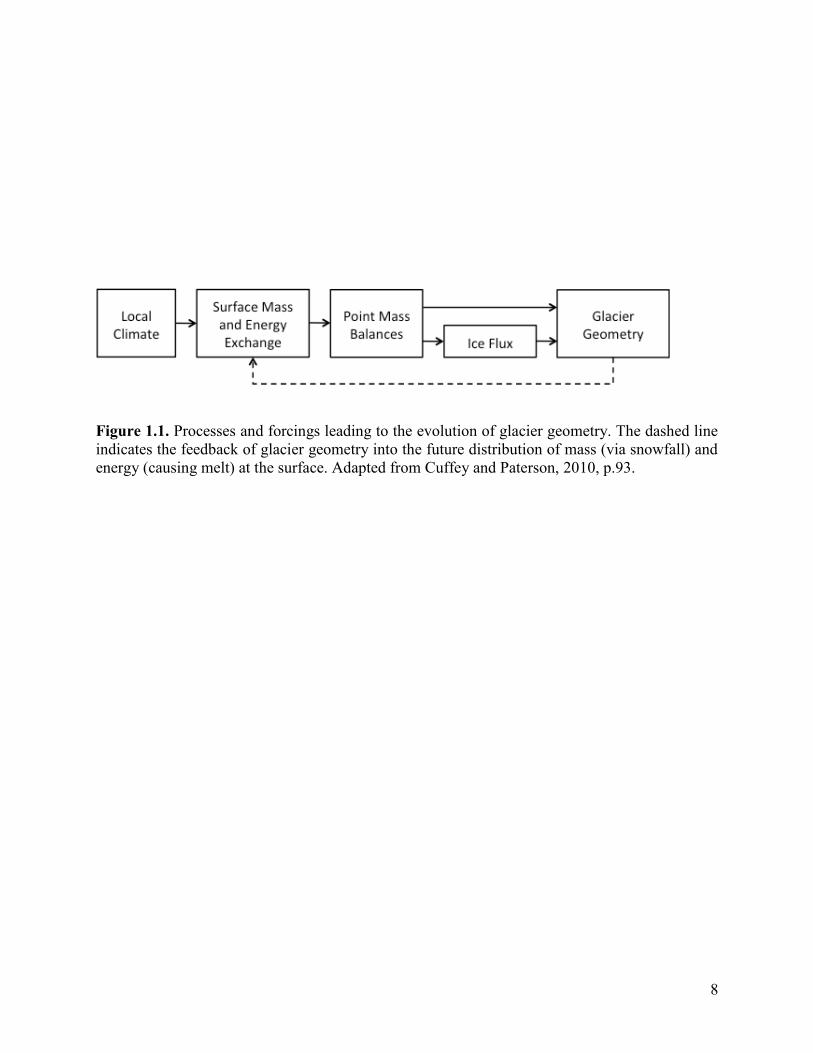
turnover rates [Furbish and Andrews, 1984]. The feedback cycle depicted in Figure 1.1 illustrates
that mass balance and ice dynamics together play a role in modifying glacier hypsometry, and
subsequently that glacier hypsometry dictates future mass balance conditions for a glacier. Mass
balance controls on hypsometry comprise elevation gain due to snowfall in the accumulation area,
and elevation loss due to surface melt in the ablation area. In an idealized case with stable climate
conditions, the transfer of mass (flux) from the accumulation area to the ablation area by ice motion
will compensate for these changes in elevation (via the continuity equation; Cuffey and Paterson
[2010]).
With a stepwise change in climate the glacier geometry should be expected to adjust, by
the mechanisms of ice motion, to a new state that is stable (in balance) in the new climate regime
[Cuffey and Paterson, 2010; Elsberg et al., 2001; Harrison et al., 2009]. The dynamics of ice
motion are, however, controlled by many internal and external factors that may lead to mass
transfers that exceed, or fail to meet, the mass flux required for a stable response of the glacier to
changes in climate. For example, on multi-decadal timescales changes in mass balance can invoke
changes in ice thickness and the surface gradient that together factor into the force balance equation
that explains the driving force behind ice motion. Conversely, short-term (hourly-daily)
fluctuations in ice motion are closely linked with the meteorologically controlled input of surface
melt water, the conditions at the glacier bed, the structure of the subglacial hydrological system

3
and the efficiency at which water leaves the system [Bartholomaus et al., 2008; Bingham et al.,
2006; Cuffey and Paterson, 2010; Sundal et al., 2011]. These long- and short-term processes can
lead to ice fluxes that exceed the balance flux and, as a result, ice will be conveyed to lower
elevations at a rate that is unsustainable in the present climate. This augmented mass transfer will
cause the accumulation area to descend into lower elevations with increasingly negative mass
balance regimes. The future stability of a glacier is therefore determined by the nature of the glacier
response to changes in climate [Harrison et al., 2009]. Examples of recently observed unstable
glacier response to climate warming are Yakutat and Brady glaciers in southeast Alaska, where
significant ice thinning at higher elevations has ultimately removed the accumulation areas of these
glaciers and resulted in unsustainable hypsometries for glacier mass balance [Harrison et al.,
2009].
While previous studies have used energy balance models to predict future mass balance
conditions [Lenaerts et al., 2013; Oerlemans et al., 2005], the stability of the physical response of
Arctic mountain glaciers to accelerating climate warming has yet to be investigated. Recent
climate and mass balance modeling results predict an irreversible mass loss for glaciers in the
Canadian Arctic under future climate projections [Lenaerts et al., 2013]. However, if these glaciers
assume new hypsometries that are stable in the contemporary climate, the findings of Lenaerts et
al. [2013] do not necessarily imply that these glaciers are destined to disappear. This distinction is
important to note because while the projected warming would force Arctic glaciers into high
elevation basins following significant volume losses, the persistence of small ice masses
throughout the year would hold important implications for sustained streamflow in these
watersheds through the summer months and for the riparian ecosystems that depend of them. The
future of Arctic glaciers therefore depends on their ability to dynamically adjust their geometries
to elevations and extents that are sustainable under projected climate conditions.
Since early mapping campaigns in the CAA during the 1950s and 1960s, the response of
glacier and ice cap geometry to the decreasing mass balance trend has been one of retreat and
varying degrees of thinning, particularly on small stagnating glaciers and ice caps [Braun et al.,
2004a; Papasodoro et al., 2015; Thomson et al., 2011]. Thinning due to ablation is known as
downwasting, whereas dynamic thinning occurs as a result of a positive flux divergence, where
more ice flows out of a given region than flows in [Cogley et al., 2011b]. Thinning can also occur
in the accumulation area as a result of changes to the amount and form of precipitation [Screen

4
and Simmonds, 2012], as well as the rate of snow densification [Morris and Wingham, 2011].
Processes of thinning that cause glaciers to assume a hypsometry with more area at lower
elevations will likely initiate a positive feedback as more of the glacier area is lowered into
negative mass balance conditions (Figure 1.1). By understanding the relative contribution to
changes in glacier geometry from each of these processes, it may be possible to improve
predictions of the future response of Arctic mountain glaciers.
1.2 FOCUS AND OBJECTIVES
This thesis investigates how climate conditions over the past half-century have impacted
the response of White Glacier, an alpine glacier on Axel Heiberg Island in the Canadian High
Arctic. White Glacier is currently the only mountain glacier (i.e., not an ice cap or outlet glacier)
in the CAA with in situ measurements of mass balance and ice dynamics spanning multiple
decades. While mountain glaciers generally comprise a minority of glacier-covered area in the
CAA (e.g. 26% on Axel Heiberg Island), they demonstrate a greater sensitivity to climate warming
both in terms of area change and mass balance [Dowdeswell et al., 1997; Paul, 2004; Thomson et
al., 2011]. Therefore, this study of White Glacier’s mass balance and dynamics serves as an
indicator of how glaciers in the alpine environment are responding to Arctic amplification in the
CAA. Using historic datasets dating back to 1960, this work presents a multi-decadal assessment
of mass balance, dynamics, and hypsometry of the glacier through comparison of early and
contemporary glaciological datasets including large-scale maps, a 56-year mass balance record,
englacial temperature measurements, local climate observations, and measurements of seasonal
and annual ice velocities from 1960–1970 and 2012–2016.
The first objective of this thesis is to produce an updated map of White Glacier from which
changes in ice thickness and glacier hypsometry can be determined. Using >400 oblique aerial
photographs collected in July 2014, a new digital elevation model (DEM) was created using
Structure from Motion techniques, a method built upon traditional photogrammetry but with the
advantage of automated image correlation analysis. The result of this work demonstrates that the
Structure from Motion method is able to overcome the challenges of optical remote sensing in
low-contrast, snow-covered areas due to the high resolution of the photographs and their
subsequent detection of small features at the surface. The resulting DEM and orthoimage
5
facilitated the production of a new 1:10,000 topographic map with 5 m vertical accuracy in the
style of earlier cartographic works of White Glacier dating back to 1960.
The second objective is to assess how changing glacier geometry (hypsometry and extent)
impacts the calculation of glacier mass balance. The impact of glacier thinning and glacier retreat
have contrasting impacts on the calculation of glacier mass balance; the former promotes
increasingly negative mass balance as more mass is exposed to warmer temperatures at lower
elevations, whereas the latter results in the removal of the portion of the glacier where the most
extreme loss is experienced, resulting a less negative mass balance overall. The new map created
in the first part of the thesis enabled calculation of the glacier’s geodetic mass balance (mass
change determined from ice volume change) and provides an updated glacier hypsometry that
improves the accuracy of contemporary mass balance calculations. A modeled glacier hypsometry
time series was created to support a reanalysis of the mass balance record [Zemp et al., 2013],
which through comparison of the geodetic and glaciological methods enabled the estimation of
generic differences (i.e. discrepancies between total and surface mass balance) and potential
sources of error in the glaciological method.
The third objective of this thesis is to provide a determination of how ice dynamics have
responded to a trend of ice thinning and increasingly negative mass balance conditions at White
Glacier. To address this objective, dual-frequency GPS (dGPS) stations were installed at the centre
of three cross-sectional profiles to continuously monitor ice motion from 2012–2016. These sites
were the focus of previous surface velocity measurements from 1960–1970 [Iken, 1974; Müller
and Iken, 1973]. Post-processing of the dGPS data following the approach of the earlier
observations, which enables comparison of annual, winter and summer velocities at each of the
three stations. Modeling of expected glacier velocities using theoretical balance velocities and
Glen’s flow law are used to assess the relative roles of mass balance and hypsometry changes (i.e.
ice thinning) in the observed changes in glacier velocity.
1.3 STUDY LOCATION AND REGIONAL CLIMATE
White Glacier (79.4º N, 90.6º W) is a 14 km long mountain glacier extending from
approximately 100 to 1800 m a.s.l. in the region of Expedition Fiord on western Axel Heiberg
Island in the Queen Elizabeth Islands of the Canadian High Arctic (Figure 1.2). The glacier has a

6
5 km wide accumulation area and flows southeast into a narrow 0.8-1.1 km wide valley. Over the
period of observation (1960–2015), the average equilibrium line altitude was 1075 m a.s.l. and the
mean accumulation area ratio (accumulation area divided by the total area) was 0.55. The glacier
area in 1960 was 41.07 km2, which decreased to 38.54 km2 by 2014 [Thomson and Copland, 2016].
White Glacier terminates at a junction with Thompson Glacier, a major outlet glacier of the Müller
Ice Cap.
The glaciers on Axel Heiberg Island, numbering 1108 in 1960 [Ommanney, 1969], range
from large outlet glaciers (>100 km2) to small mountain and niche-type ice masses observed to
have decreased in area by 50-80% between 1960 and 2000 [Thomson et al., 2011]. The two major
ice caps on the island are the Müller Ice Cap, located 50 km northeast of Expedition Fiord
(maximum elevation 2210 m a.s.l. at Outlook Peak) and the Steacie Ice Cap on the southern half
of the island, approximately 70 km south of White Glacier. The Müller Ice Cap was named in
honour of Dr. Fritz Müller of McGill University who initiated the glacier monitoring activities in
the Expedition Fiord regions, and who founded the McGill Arctic Research Station as part of the
Jacobsen-McGill Arctic Research Expedition 1959-1962.
The region experiences mean annual temperatures of approximately –20°C and annual
precipitation ranging from 58 mm a-1 at sea level (as measured at Eureka, 125 km to the northeast)
to 370 mm a-1 at 2120 m a.s.l. as measured in a 41-year snowpit record of annual accumulation on
the Müller Ice Cap [Cogley et al., 1996]. There are no continuous measurements of local climate
conditions in the Expedition Fiord region, although several early studies based at the McGill Arctic
Research Station include periodic climate data (e.g. Andrews, 1964; Havens et al., 1965). A
significant amount of climate data is also available in Ohmura [1981], which presents the first
detailed energy balance model of the high-arctic that accounts for the interactions between
glaciers, tundra, and sea ice [Cogley et al., 1996].
The closest weather stations with near-continuous climate data are the Eureka Weather
Station, located approximately 125 km to the northeast on Ellesmere Island, and Isachsen station
situated 275 km to the southwest on Ellef Ringnes Island. An analysis of the long-term climate
record at Eureka (1954-2007) by Lesins et al. [ 2010] shows that mean annual surface temperatures
have risen there by 3.2°C since 1972 and that the most significant warming has occurred during
the winter months. A 10% increase in total annual precipitation, predominantly during the spring,
summer and autumn months, was also observed over the period of record. Figure 1.3 presents the

7
mean annual air temperature and precipitation data for Eureka and Isachsen, acquired from
Environment Canada’s Historical Climate Data pages: www.climate.weather.gc.ca/historical_data
From these records, a period of cooling temperatures in the 1970s is apparent at both
stations, which may correlate with increasing precipitation at the Isachsen station. Since the 1970s,
the Eureka temperature data follow the warming trend indicated by Lesins et al. [2010]. A warming
trend also appears likely in the Isachsen record given contemporary measurements, despite a gap
in the data between 1978 and 2003. Given these observations at stations to the east and west of
Axel Heiberg Island, it is likely that the region of Expedition Fiord has experienced similar
warming since the 1970s and that this warming explains the increasingly negative mass balance
conditions observed in recent decades (Figure 3.2). While an increase in precipitation has occurred
at Eureka, mass balance records show no apparent increase in accumulation rates on White Glacier
over the period of record (1960-2015). This is potentially related to the difference in elevation
between the Eureka observing station (~10 m a.s.l.) and the accumulation area of White Glacier
(~1200-1800 m a.s.l.), as well as distance from moisture sources such as the Arctic Ocean.
1.4 THESIS FORMAT
The thesis follows a manuscript-style format in which three articles are developed. An
introductory chapter (Chapter 1) synthesizes the scientific literature that has motivated this work
and presents the thesis objectives. Chapters 2-4 (the articles) open with an attestation statement
indicating the individual contributions of coauthors and the current status of the article in the
publication process. A certain degree of repetition is present between the three papers in the
sections concerning previous studies and description of the study site. At the end of each chapter
the associated tables and figures are provided. Chapter 5 presents the combined findings of these
articles. It highlights overall implications for the stability of the response of White Glacier under
the current climate and places these findings in the context of other studies relating to glacier mass
balance and ice dynamics. The references for all chapters are provided together in Chapter 6.
8
Figure 1.1. Processes and forcings leading to the evolution of glacier geometry. The dashed line
indicates the feedback of glacier geometry into the future distribution of mass (via snowfall) and
energy (causing melt) at the surface. Adapted from Cuffey and Paterson, 2010, p.93.

9
Figure 1.2. Regional map of the Queen Elizabeth Islands, including the locations of the Eureka
and Isachsen weather stations, respectively 125 km northeast and 275 km southwest of Expedition
Fiord on Axel Heiberg Island (shown in the inset map).
100 W
80 N

10
Figure 1.3. Mean annual air temperature (°C) and total annual precipitation (mm) for the Eureka
and Isachsen Environment Canada weather stations.
11
CHAPTER 2: GLACIER MAPPING USING STRUCTURE FROM MOTION
2.1 ARTICLE 1 SUMMARY AND ATTESTATION
We use Structure from Motion software to generate a new digital elevation model (DEM)
of White Glacier, Axel Heiberg Island, Nunavut, using >400 oblique aerial photographs collected
in July 2014. Spatially and radiometrically high-resolution imagery, optimized camera settings,
low angle lighting conditions, and image post-processing methods together supported the detection
of small but distinct features on the surface of the snowpack and enabled feature matching during
the image correlation process. The resulting DEM and orthoimage facilitated the production of a
new 1:10,000 topographic map with 5 m vertical accuracy in the style of earlier cartographic works
of White Glacier dating back to 1960. The new map of White Glacier will support calculation of
the glacier’s geodetic mass balance (mass change determined from ice volume change over the
past 54 years) and provides an updated glacier hypsometry (area-elevation distribution) that will
improve the accuracy of future mass balance calculations.
Laura Thomson and Luke Copland, respectively, co-authored an article entitled “White
Glacier 2014, Axel Heiberg Island, Nunavut: mapped using Structure from Motion methods”
based on this chapter. Laura Thomson was responsible for the data collection, post-processing,
topographic model building, map development, and initial authorship of this article. Luke Copland,
along with three reviewers from the Journal of Maps, provided helpful revisions that have resulted
in the following publication:
Thomson, L. and Copland, L. 2016. White Glacier 2014, Axel Heiberg Island, Nunavut: mapped
using Structure from Motion methods. Journal of Maps. doi: 10.1080/17445647.2015.1124057.
2.2 INTRODUCTION
White Glacier (79.45° N, 90.67° W, Figure 2.1) on Axel Heiberg Island, Nunavut, has been
the subject of glaciological studies in Canada’s north since 1959 and today hosts the longest mass
balance record for an alpine glacier in the Canadian Arctic (55 years). It is one of 37 official
reference glaciers within the Global Terrestrial Network for Glaciers through the United Nations
Framework Convention on Climate Change. These observations, submitted annually to the World
12
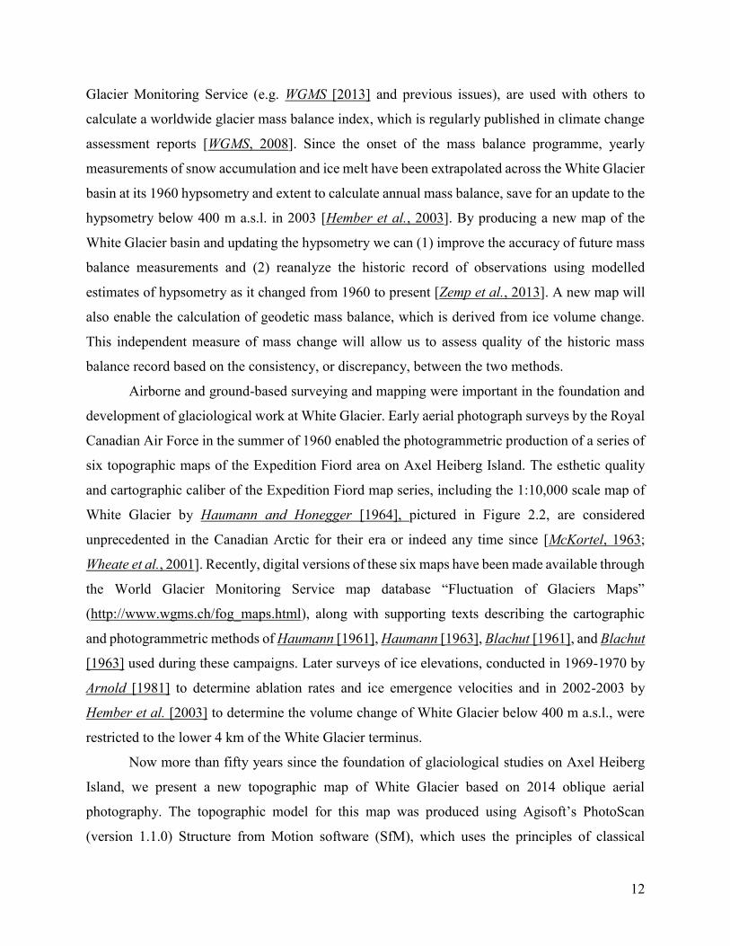
Glacier Monitoring Service (e.g. WGMS [2013] and previous issues), are used with others to
calculate a worldwide glacier mass balance index, which is regularly published in climate change
assessment reports [WGMS, 2008]. Since the onset of the mass balance programme, yearly
measurements of snow accumulation and ice melt have been extrapolated across the White Glacier
basin at its 1960 hypsometry and extent to calculate annual mass balance, save for an update to the
hypsometry below 400 m a.s.l. in 2003 [Hember et al., 2003]. By producing a new map of the
White Glacier basin and updating the hypsometry we can (1) improve the accuracy of future mass
balance measurements and (2) reanalyze the historic record of observations using modelled
estimates of hypsometry as it changed from 1960 to present [Zemp et al., 2013]. A new map will
also enable the calculation of geodetic mass balance, which is derived from ice volume change.
This independent measure of mass change will allow us to assess quality of the historic mass
balance record based on the consistency, or discrepancy, between the two methods.
Airborne and ground-based surveying and mapping were important in the foundation and
development of glaciological work at White Glacier. Early aerial photograph surveys by the Royal
Canadian Air Force in the summer of 1960 enabled the photogrammetric production of a series of
six topographic maps of the Expedition Fiord area on Axel Heiberg Island. The esthetic quality
and cartographic caliber of the Expedition Fiord map series, including the 1:10,000 scale map of
White Glacier by Haumann and Honegger [1964], pictured in Figure 2.2, are considered
unprecedented in the Canadian Arctic for their era or indeed any time since [McKortel, 1963;
Wheate et al., 2001]. Recently, digital versions of these six maps have been made available through
the World Glacier Monitoring Service map database “Fluctuation of Glaciers Maps”
(http://www.wgms.ch/fog_maps.html), along with supporting texts describing the cartographic
and photogrammetric methods of Haumann [1961], Haumann [1963], Blachut [1961], and Blachut
[1963] used during these campaigns. Later surveys of ice elevations, conducted in 1969-1970 by
Arnold [1981] to determine ablation rates and ice emergence velocities and in 2002-2003 by
Hember et al. [2003] to determine the volume change of White Glacier below 400 m a.s.l., were
restricted to the lower 4 km of the White Glacier terminus.
Now more than fifty years since the foundation of glaciological studies on Axel Heiberg
Island, we present a new topographic map of White Glacier based on 2014 oblique aerial
photography. The topographic model for this map was produced using Agisoft’s PhotoScan
(version 1.1.0) Structure from Motion software (SfM), which uses the principles of classical

13
photogrammetry and takes advantage of computer automated image correlation analysis [Jebara
et al., 1999]. In recognition of the merit of the first 1:10,000 scale map of White Glacier by
Haumann and Honegger [1964] we have strived to mimic the design features and quality of the
original in our own map, while accepting the fundamental differences between hand-drawn and
digital cartographic methods.
2.3 METHODS
2.3.1 AERIAL PHOTOGRAPH SURVEY AND IMAGE POST-PROCESSING
A Canon EOS 6D digital SLR camera equipped with an EF 24-105mm f4 L IS USM lens
(set to a fixed focal length of 24 mm) was used to collect >500 oblique photographs of White
Glacier from the open window of a Bell 206L helicopter on July 10, 2014. At an average flying
height of 1645 m above sea level (a.s.l.) (~5400 ft.), and a maximum altitude of 1990 m a.s.l.
(~6525 ft.) over the accumulation area, the camera achieved ground resolutions ranging from 0.05
to 0.52 m based on photographs with a resolution of 3648 x 5472 pixels (20 Megapixels). An
automatic intervalometer programmed to capture images every 3 seconds enabled 80% image
overlap along-track and 60% across-track at an average flying speed of ~150 km hr-1, as
recommended in AgiSoft PhotoScan (hereafter, PhotoScan) User Manual and by Dr. Matt Nolan
(personal communication, 2014).
At the start of the survey, a reconnaissance flight was conducted over the Crusoe Glacier
accumulation area (Figure 2.3a) to adjust the camera to settings that could detect features from the
brightest part of the image (i.e., snow under direct sunshine). On the camera screen we were able
to view the image exposure and RGB histograms on test photographs; through trial and error we
found that camera settings of F-stop=F/10, ISO=100 and a fixed shutter speed of 1/2500 allowed
for maximum contrast and detection of snow features across the accumulation area. These features
included ripple marks (Figure 2.3b) and sastrugi, which were enhanced by high-elevation surface
melt and low angle lighting, as well as small slush avalanches and meltwater streams originating
near nunataks. The low exposure camera settings resulted in good definition in the accumulation
area at the expense of under exposure in other locations, particularly in shadowed areas in the
western tributary basins of White Glacier. However, the 14-bit radiometric resolution of the Canon
EOS 6D enables over 16,000 tones to be uniquely identified, which supported the detection of

14
subtle features in both snow-covered and shadowed regions. Using Canon Digital Photo
Professional (version 3.12.51.2) photo editing software, the image brightness was increased by
30%, maintaining definition in the accumulation area while enhancing contrast in the shadowed
regions of the glacier (Figure 2.3c). Batch post-processing was applied to ensure continuity in
lighting throughout the photo series.
2.3.2 Model Building
The Structure from Motion approach used by PhotoScan differs from traditional digital
photogrammetry in that the image correlation analysis is used not only to derive three-dimensional
structure from measureable feature offsets between images (i.e. parallax), but also to infer the
camera position and calibration parameters of each photograph. This reduces the processing time
required and enables projects to involve hundreds of photographs. Construction of a topographic
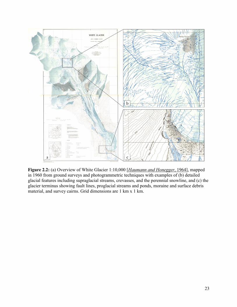
model in PhotoScan is a multi-step process, as illustrated in Figure 2.4. Several iterations of model
building for White Glacier were run before the final results were achieved; here, we describe the
parameter settings and method used to produce the final product.
With the reference projection defined as NAD27, the post-processed photographs were
imported into PhotoScan and inspected for image coverage and quality, resulting in 473
photographs that were used to build the final model. Manually delineated image masks were
applied to the photos to exclude features such as clouds and distant terrain outside the White
Glacier basin that would interfere with photo alignment. In PhotoScan, photo alignment refers to
the process in which a user-defined number of tie-points, detected by correlation analysis between
two photos, and camera orientation and positions are determined in 3D space using a bundle
adjustment (PhotoScan User Manual). The resulting 3D point cloud calculated for a pair of images
is referred to as a depth map, and PhotoScan amalgamates these depth maps to produce sparse
point cloud for the entire 3D structure to be modelled (PhotoScan User Manual). The most
intensive and iterative phase of model building was adjusting and improving the photo alignment
by the manual addition and removal of tie points and ground control points (discussed in Section
2.4) and the deletion of erroneous points with high reprojection errors. In PhotoScan, reprojection
error is a measure of localization accuracy in pixels. The standard assumption is that an “average
reprojection error higher than 0.8 pix indicates quite inaccurate solution. Whereas reprojection
error less than 0.5 is almost perfect” (Agisoft Technical Support). The final sparse point cloud
15
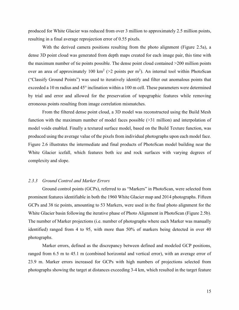
produced for White Glacier was reduced from over 3 million to approximately 2.5 million points,
resulting in a final average reprojection error of 0.55 pixels.
With the derived camera positions resulting from the photo alignment (Figure 2.5a), a
dense 3D point cloud was generated from depth maps created for each image pair, this time with
the maximum number of tie points possible. The dense point cloud contained >200 million points
over an area of approximately 100 km2 (>2 points per m2). An internal tool within PhotoScan
(“Classify Ground Points”) was used to iteratively identify and filter out anomalous points that
exceeded a 10 m radius and 45° inclination within a 100 m cell. These parameters were determined
by trial and error and allowed for the preservation of topographic features while removing
erroneous points resulting from image correlation mismatches.
From the filtered dense point cloud, a 3D model was reconstructed using the Build Mesh
function with the maximum number of model faces possible (>31 million) and interpolation of
model voids enabled. Finally a textured surface model, based on the Build Texture function, was
produced using the average value of the pixels from individual photographs upon each model face.
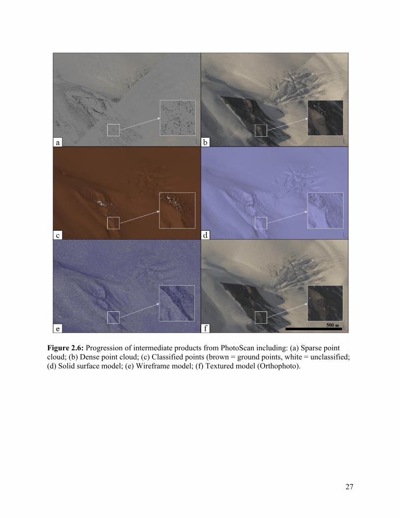
Figure 2.6 illustrates the intermediate and final products of PhotoScan model building near the
White Glacier icefall, which features both ice and rock surfaces with varying degrees of
complexity and slope.
2.3.3 Ground Control and Marker Errors
Ground control points (GCPs), referred to as “Markers” in PhotoScan, were selected from
prominent features identifiable in both the 1960 White Glacier map and 2014 photographs. Fifteen
GCPs and 38 tie points, amounting to 53 Markers, were used in the final photo alignment for the
White Glacier basin following the iterative phase of Photo Alignment in PhotoScan (Figure 2.5b).
The number of Marker projections (i.e. number of photographs where each Marker was manually
identified) ranged from 4 to 95, with more than 50% of markers being detected in over 40
photographs.
Marker errors, defined as the discrepancy between defined and modeled GCP positions,
ranged from 6.5 m to 45.1 m (combined horizontal and vertical error), with an average error of
23.9 m. Marker errors increased for GCPs with high numbers of projections selected from
photographs showing the target at distances exceeding 3-4 km, which resulted in the target feature

16
being at a compromised resolution. However, we believed it to be important to incorporate as many
projections as possible for each GCP to ensure continuity in the model.
2.3.4 Model Results
We found that the SfM model construction generally performed well across the White
Glacier basin, and surprisingly so across the accumulation area. The combination of low exposure
settings, high spatial and radiometric-resolution photography, low angle lighting, and the onset of
summer surface melt generally resulted in successful feature matching and model construction
throughout the snow-covered regions.
Erroneous sections of the model were found to be associated primarily with failures in
survey design and photo coverage, rather than issues with the model building process. For
example, two basins in the northeastern accumulation area of the glacier returned “pitted” results,
i.e., regions of elevations significantly below (up to 100 m) the actual surface. In this case, image
coverage of these basins was compromised by the eclipsing effect of ridges in the foreground of
the oblique photographs. In another example, we found that along the western margin of the glacier
trunk the model had difficulty transitioning smoothly from illuminated to shadowed lighting
conditions, resulting in an artificial terrace in this region. Significant efforts were made to remedy
this issue, including (1) adjusting the brightness and contrast parameters, (2) the inclusion of tie
points, and (3) adjusting the selection parameters for ground points, but these proved to be
ineffective. These two cases exemplify the most extreme and extensive model errors, yet together
they comprise only 3% of the mapped basin area. Smaller isolated instances of “pitting” on the
scale of 50-400 m in length appear primarily in the accumulation area, and in some cases appear
to be associated with variable cloud coverage between photographs. Our approach to managing
these issues is addressed in Section 2.4.2, which describes contour construction and design.
The resulting 3D model and textured surface were exported as a DEM and orthophoto,
respectively. The default model export cell size provided by Agisoft was 0.769 m, but we chose to
export the DEM at a resolution of 5 m to reduce the impact of small-scale noise and variability on
contour construction. The orthophoto was exported at a resolution of 1 m to facilitate the detailed
mapping of small-scale features such as supraglacial streams and crevasses.
17
2.4 MAP CONSTRUCTION AND DESIGN
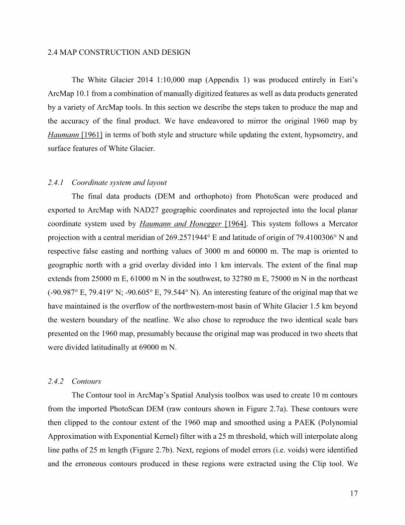
The White Glacier 2014 1:10,000 map (Appendix 1) was produced entirely in Esri’s
ArcMap 10.1 from a combination of manually digitized features as well as data products generated
by a variety of ArcMap tools. In this section we describe the steps taken to produce the map and
the accuracy of the final product. We have endeavored to mirror the original 1960 map by
Haumann [1961] in terms of both style and structure while updating the extent, hypsometry, and
surface features of White Glacier.
2.4.1 Coordinate system and layout
The final data products (DEM and orthophoto) from PhotoScan were produced and
exported to ArcMap with NAD27 geographic coordinates and reprojected into the local planar
coordinate system used by Haumann and Honegger [1964]. This system follows a Mercator
projection with a central meridian of 269.2571944° E and latitude of origin of 79.4100306° N and
respective false easting and northing values of 3000 m and 60000 m. The map is oriented to
geographic north with a grid overlay divided into 1 km intervals. The extent of the final map
extends from 25000 m E, 61000 m N in the southwest, to 32780 m E, 75000 m N in the northeast
(-90.987° E, 79.419° N; -90.605° E, 79.544° N). An interesting feature of the original map that we
have maintained is the overflow of the northwestern-most basin of White Glacier 1.5 km beyond
the western boundary of the neatline. We also chose to reproduce the two identical scale bars
presented on the 1960 map, presumably because the original map was produced in two sheets that
were divided latitudinally at 69000 m N.
2.4.2 Contours
The Contour tool in ArcMap’s Spatial Analysis toolbox was used to create 10 m contours
from the imported PhotoScan DEM (raw contours shown in Figure 2.7a). These contours were
then clipped to the contour extent of the 1960 map and smoothed using a PAEK (Polynomial
Approximation with Exponential Kernel) filter with a 25 m threshold, which will interpolate along
line paths of 25 m length (Figure 2.7b). Next, regions of model errors (i.e. voids) were identified
and the erroneous contours produced in these regions were extracted using the Clip tool. We
18
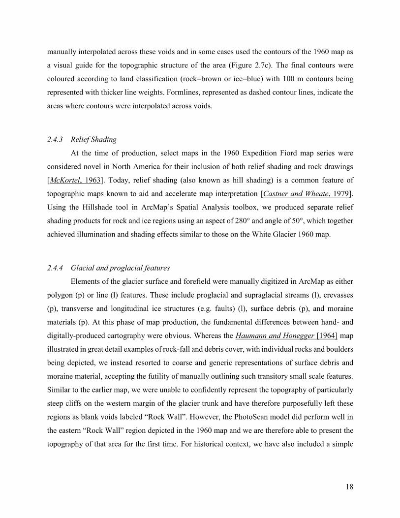
manually interpolated across these voids and in some cases used the contours of the 1960 map as
a visual guide for the topographic structure of the area (Figure 2.7c). The final contours were
coloured according to land classification (rock=brown or ice=blue) with 100 m contours being
represented with thicker line weights. Formlines, represented as dashed contour lines, indicate the
areas where contours were interpolated across voids.
2.4.3 Relief Shading
At the time of production, select maps in the 1960 Expedition Fiord map series were
considered novel in North America for their inclusion of both relief shading and rock drawings
[McKortel, 1963]. Today, relief shading (also known as hill shading) is a common feature of
topographic maps known to aid and accelerate map interpretation [Castner and Wheate, 1979].
Using the Hillshade tool in ArcMap’s Spatial Analysis toolbox, we produced separate relief
shading products for rock and ice regions using an aspect of 280° and angle of 50°, which together
achieved illumination and shading effects similar to those on the White Glacier 1960 map.
2.4.4 Glacial and proglacial features
Elements of the glacier surface and forefield were manually digitized in ArcMap as either
polygon (p) or line (l) features. These include proglacial and supraglacial streams (l), crevasses
(p), transverse and longitudinal ice structures (e.g. faults) (l), surface debris (p), and moraine
materials (p). At this phase of map production, the fundamental differences between hand- and
digitally-produced cartography were obvious. Whereas the Haumann and Honegger [1964] map
illustrated in great detail examples of rock-fall and debris cover, with individual rocks and boulders
being depicted, we instead resorted to coarse and generic representations of surface debris and
moraine material, accepting the futility of manually outlining such transitory small scale features.
Similar to the earlier map, we were unable to confidently represent the topography of particularly
steep cliffs on the western margin of the glacier trunk and have therefore purposefully left these
regions as blank voids labeled “Rock Wall”. However, the PhotoScan model did perform well in
the eastern “Rock Wall” region depicted in the 1960 map and we are therefore able to present the
topography of that area for the first time. For historical context, we have also included a simple

19
representation of the extent of the glacier terminus in 1960, as shown in the Haumann and
Honegger [1964] map.
2.4.5 Survey cairns, spot elevations, and reference prisms
Ground surveys which provided ground control for the 1960 photogrammetry project made
use of signal plates and a network of cairns, many of which were created in pairs to form survey
baselines (e.g. I.C.B.N. and I.C.B.S., which we assume to signify Ice Cave Baseline North and
South). We have chosen to include these reference points, as well as spot elevations, from the
Haumann and Honegger [1964] map in our own, making it clear in the legend that these points
are accurate as of their year of survey, 1960. It should be noted that the elevations of the 1960 spot
elevations on the ice surface will have changed as a result of ice thinning or, in the case of Signal
cairns W.G.F.4 and W.G.F.5, by the advance of Thompson Glacier into the White Glacier
Forefield (W.G.F.) from the east. Several of the signal cairns that remain were resurveyed using a
dual-frequency GPS (dGPS) system between 2011 and 2014. We include the point elevations of
these contemporary surveys with a separate symbology. In all cases, our dGPS measurements of
off-ice markers returned elevations within 1 m of those reported in Haumann and Honegger
[1964], attesting to the high precision of the early work by the Swiss and Canadian surveyors on
Axel Heiberg Island. We have added three new spot elevations at the sites of permanent reference
prisms installed for our own total station surveys (R1-R3) and two spot elevations at historic
markers we found that post-date the Haumann and Honegger [1964] map, including a
meteorological station on the White Glacier Outwash Plain ‘W.G.O.P.’ used by Atsumu Ohmura
in 1969 [Ohmura, 1981].
2.4.6 Map accuracy
As recommended by Agisoft, the standard rule of thumb for determining DEM accuracy
from ground sampling distance (GSD) is 2x GSD in the horizontal and 4x in the vertical. Therefore,
our GSD of 0.38 m (average ground resolution as calculated by PhotoScan) returns a horizontal
accuracy of 0.76 m and vertical accuracy of 1.52 m. However, we believe this to be overly
optimistic and more likely a reflection of DEM precision, not accuracy. The reported marker errors
of the PhotoScan DEM product, which reflect the discrepancy between user defined and modeled
20
GCPs, indicate average horizontal errors in longitude and latitude of 14.1 m and 16.3 m,
respectively, and an average elevation error of 10.5 m. These values, on the other hand, are subject
to the unknown errors associated with the local plane coordinate system, which is poorly defined
[Cogley and Jung-Rothenhäusler, 2002], thereby introducing further errors in the geolocation of
the model.
The majority of ground control validation in the model was acquired from off-ice survey
points and peaks with established elevations during the 1960 ground surveys. However, for the
purposes of future glaciological studies, including comparison of historic and contemporary
surfaces to determine glacier volume change, it is important to have on-ice validation of glacier
surface elevations. We used a dGPS profile collected by snow-mobile in the spring of 2014 as on-
ice validation for the 2014 DEM. Comparison of 286 point elevations acquired along the dGPS
track with the 2014 SfM DEM (Figure 2.8 a-b) show that, on average, the DEM is 1.30 m lower
than the dGPS elevations and exhibits a normal distribution (Figure 2.8 c). Scatter plots comparing
the elevation discrepancies suggest that the 2014 DEM tends to overestimate elevation at lower
elevations near the terminus and at higher elevations in the accumulation area (Figure 2.8 d-e).
One possible explanation for this pattern is that the dGPS measurements were collected during the
spring months (prior to the onset of summer 2014 melt) and would therefore reflect pre-melt
elevations at the terminus, and pre-summer lowering of the accumulated winter snow
(densification driven by melt and refreezing in the snowpack). It is also possible that there is a
warping of the model near the model edges at the glacier terminus and upper accumulation area,
however it is difficult to know how this effect might be introduced or quantified.
Ultimately, map accuracy can be considered as “the degree of conformity with a standard”
[Thompson, 1988]. To determine how well our DEM conforms to our standard, the Haumann and
Honegger [1964] map, we used the universal co-registration method developed by Nuth and Kääb
[2011] and found that the standard deviation of elevation differences over stable terrain between
our DEM and the 1960 map was 5.08 m following horizontal shifts on the order of 10-15 m. The
necessity for these shifts is likely associated with the uncertainty in the estimated parameters of
the local plane coordinate system and not inaccuracies in the DEM, considering the low
reprojection error of 0.55 pixels that we were able to achieve in PhotoScan. With these
considerations, we believe a reasonable generalization for the accuracy of the map to be 10 m
vertically and 5 m horizontally.

21
2.5 CONCLUSIONS
Through the use of SfM photogrammetry methods applied to >400 oblique air photos, we
have produced a DEM and orthoimage that together provide the foundation for a new 1:10,000
topographic map of White Glacier. Image correlation over the snow-covered areas of the glacier
was possible due to the low-exposure camera settings, favorable lighting conditions, and melt
season survey that enabled the detection of small-scale snow-surface features. Challenges faced in
the process, which resulted in some localized model errors, were largely associated with flight
survey design and uncertainties in the local plane coordinate system. Provided the opportunity to
apply this technique in the future, nadir-oriented photography acquired from a greater flying height
would resolve the issue of eclipsed regions, and map accuracy could be improved by the placement
of more photo-identifiable GCPs. The co-registration technique developed by Nuth and Kääb
[2011] provides an important tool in overcoming the coordinate system uncertainties of the
Haumann and Honegger [1964] map as we move forward in calculating the volume change of
White Glacier between 1960 and 2014 in future studies.
22
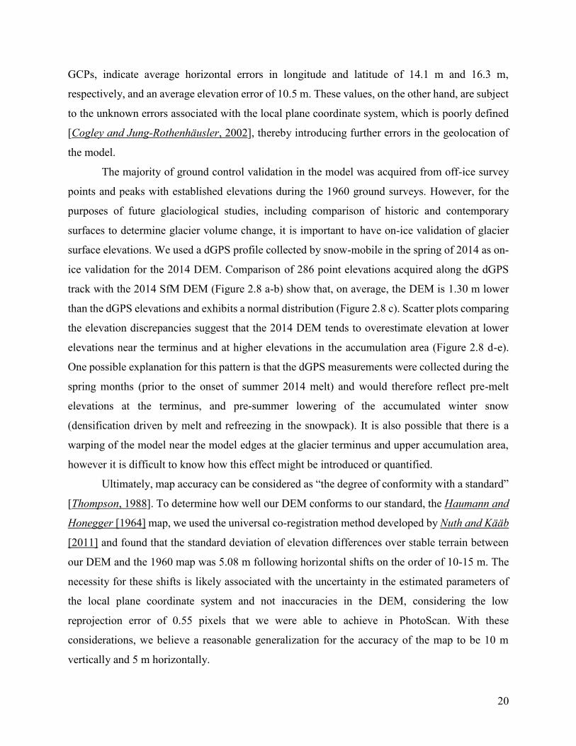
Figure 2.1: Location of White, Crusoe, Thompson, and Baby glaciers in the region of
Expedition Fiord, Axel Heiberg Island (AHI). Survey baseline points Astro 1 and Astro 2 are
indicated, as is the location of the McGill Arctic Research Station (MARS). Background image:
ASTER L1B composite, July 5, 2010.
23
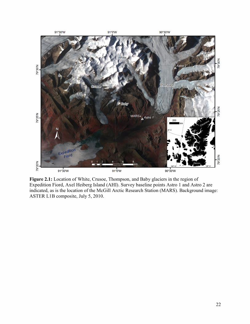
Figure 2.2: (a) Overview of White Glacier 1:10,000 [Haumann and Honegger, 1964], mapped
in 1960 from ground surveys and photogrammetric techniques with examples of (b) detailed
glacial features including supraglacial streams, crevasses, and the perennial snowline, and (c) the
glacier terminus showing fault lines, proglacial streams and ponds, moraine and surface debris
material, and survey cairns. Grid dimensions are 1 km x 1 km.

24
Figure 2.3: (a) Survey path on July 10, 2014, illustrating northbound flights in red, southbound
flights in blue, and reconnaissance flight indicated in orange. (b) Example of sastrugi present in
the accumulation of White Glacier with field team conducting snow pit analysis in foreground.
(c) Provides an example survey photo demonstrating the detail and contrast possible from the
accumulation area in both snow covered and shadowed regions.
25
Figure 2.4: Workflow for the White Glacier model construction using Agisoft PhotoScan
Structure from Motion Software.

26
Figure 2.5: (a) Camera positions derived from the Photo Alignment bundle adjustment phase in
Agisoft PhotoScan. Black lines indicate camera pointing direction and blue represents the
camera faces. The Y-axis indicates geographic north. (b) Markers used to aid in Photo Alignment
with red Markers indicating GCPs and yellow markers indicating TPs. The white box indicates
the location of the White Glacier icefall shown in Figure 2.6.
27
Figure 2.6: Progression of intermediate products from PhotoScan including: (a) Sparse point
cloud; (b) Dense point cloud; (c) Classified points (brown = ground points, white = unclassified;
(d) Solid surface model; (e) Wireframe model; (f) Textured model (Orthophoto).

28
Figure 2.7: (a) Raw contours shown in black (10 m interval); (b) Smoothed contours with region
of model errors highlighted in yellow; (c) Manually interpolated contours shown as red dashed
lines overlaid on an inset of the Haumann and Honegger (1964) map in the region of error.
Contour interval = 10 m.

29
Figure 2.8: (a) Elevations along a glacier centreline profile derived from the summer 2014 SfM
DEM (yellow) and the spring 2014 dGPS observations and (b) discrepancies (dH) along the
glacier centreline derived from differencing the 2014 DEM and dGPS measurements. The
distribution of dH values shows a normal distribution with a mean of -1.30 m. Scatter plot (d)
indicates the pattern of dH with elevation. (e) Location dGPS measurements along White
Glacier, collected in April 2014.
e

30
CHAPTER 3: MASS BALANCE REANALYSIS
3.1 ARTICLE 2 SUMMARY AND ATTESTATION
This study presents the first reanalysis of a long-term glacier mass balance record in the
Canadian Arctic. The reanalysis is accomplished through comparison of the 1960-2014
glaciological mass balance record of White Glacier, Axel Heiberg Island, Nunavut, with a
geodetically derived mass change over the same period. The corrections required to homogenize
the two datasets, including adjusting for changes in hypsometry over the period of record and the
generic differences between methods, are discussed along with the associated systematic and
random errors of the two forms of mass-balance estimation. Statistical comparison of the two
datasets reveals that within the error margin there is no significant difference between the average
annual glaciological balance (–213 ± 28 mm w.e. a-1) and geodetic balance (–178 ± 16 mm w.e.
a-1) at White Glacier over the 54-year record. The validity of this result, and the assumptions made
in implementing the glaciological method, are critically assessed.
The following chapter forms the basis for an article coauthored by Laura Thomson
(University of Ottawa), Michael Zemp (World Glacier Monitoring Service), Luke Copland
(University of Ottawa), Graham Cogley (Trent University), and Miles Ecclestone (Trent
University). The mass balance record at White Glacier, spanning 56 years (as of 2016), results
from the efforts of many field scientists including those who worked under the leadership of Fritz
Müller from 1960 to 1980, members of the Trent University Geography department from 1983 to
present, and participants from the University of Ottawa (L. Thomson, L. Copland, and M. Hackett)
in recent years. The reanalysis presented here was conducted by Laura Thomson under the
mentorship of Michael Zemp during a 5-month internship at the World Glacier Monitoring Service
at the University of Zurich (Zurich, Switzerland). Helpful revisions of the initial manuscript
written by L. Thomson were provided by the co-authors, as well as by E. Thibert and an
anonymous reviewer for the Journal of Glaciology.
Thomson, L. I., M. Zemp, L. Copland, J. G. Cogley, and M. A. Ecclestone (2016), Comparison of
Geodetic and Glaciological Mass Budgets for White Glacier, Axel Heiberg Island, NU, Journal of
Glaciology, accepted Aug. 2016..
31
3.2 INTRODUCTION
The Canadian Arctic Archipelago (CAA) hosts the largest volume of ice outside of the ice
sheets [Pfeffer et al., 2014] and occupies latitudes that are currently experiencing some of the
greatest rates of climate warming [Sharp et al., 2011; Sharp et al., 2015], a tendency that is
predicted to continue well into the future [Kirtman et al., 2013; Lenaerts et al., 2013]. A recent
analysis of the CAA in situ surface mass balance records indicates that the average glacier mass
balance between 2005 and 2009 was five times more negative than the average from 1963 to 2004
[Sharp et al., 2011]. Through modelling and remote sensing, Gardner et al. [2011] showed that
92% of the mass loss from the CAA can be explained by increased melt, while only 8% is
attributable to frontal ablation (i.e. calving) between 2004 and 2009.
In terms of estimating glacier mass balance in alpine basins, there are two primary methods:
the glaciological method (also often referred to as the direct method) involves interpolation
between in situ measurements of accumulation and ablation at stakes drilled into the glacier
surface. These stakes are typically located along the glacier centreline, and interpolation across the
glacier basin is undertaken either by assuming that mass balance varies only with elevation (the
profile method) or by mapping accumulation and ablation patterns (the contour method) [Østrem
and Brugman, 1991].
The geodetic method differences elevation models to determine changes in ice volume over
time. Estimates of the density of the ice/snowpack are then used to convert this volume change to
mass loss or gain. At the present day, these elevation models are often derived from airborne or
satellite remote sensing. Laser altimeter data from ICESat have provided a valuable resource to
determine recent ice volume changes in the CAA [Gardner et al., 2011]. However, such data does
not work well for relatively small alpine glaciers. Mass changes can also be determined using the
gravimetric method over large ice caps and ice sheets (e.g., using data from the Gravity Recovery
and Climate Experiment; Sharp et al. [2011]), but these measurements lack sufficient spatial
resolution to detect changes at the scale of alpine glacier basins.
Remote sensing methods are promising for future glacier mass balance monitoring, but to
detect and understand climatic trends in context we require earlier datasets for comparison. Surface
mass balance estimates using the glaciological method began in 1959 across the Queen Elizabeth
Islands (QEI) of the northern CAA and primarily focused on two smaller ice caps (Melville and

32
Meighen), two outlet basins of larger ice caps (Devon and Agassiz), and two mountain glaciers
(White and Baby, Axel Heiberg Island). Intermittent observations were also conducted for many
years on Ward Hunt Ice Rise and Ice Shelf on northern Ellesmere Island and Prince of Wales
Icefield on SE Ellesmere Island [Braun et al., 2004b; Hattersley-Smith and Serson, 1970; Koerner,
2005; Mair et al., 2009]. Those records submitted to the World Glacier Monitoring Service
(WGMS) and exceeding 10 years in length are shown in Figure 3.1a. Due to the large area of ice
in the QEI (~104000 km2; Sharp et al. [2014]) and logistical barriers, the CAA is comparatively
under-sampled in contrast to some other Arctic regions (e.g. Iceland, Svalbard, northern
Scandinavia; Sharp et al. [2011]). As such, it is particularly important to periodically assess the
validity of these key measurements, which have served as in situ constraints for numerous other
studies, through periodic reanalysis of the glaciological mass balance datasets [Zemp et al., 2013].
The comparison of mass-balance data series obtained by the glaciological method with
independently derived estimates of mass change offers insight into the completeness and accuracy
of the measurements [Cogley, 2009; Østrem and Haakensen, 1999; Zemp et al., 2013]. While the
glaciological method excels in capturing the large temporal and spatial variability of climate–
glacier processes, the method is also subject to biases that might be small on an annual basis but
can compound to cause significant errors over multi-decadal records. Whereas random errors rise
proportionally to the square root of the number of years, systematic biases sum linearly from year
to year. The biases are associated with the inherent limitations of the glaciological method,
primarily the challenge of measuring superimposed ice and internal accumulation, and are often
undetectable within the random error margin that is approximated to be 200 mm w.e. a-1 (w.e.,
water equivalent) for most glaciological balance measurements [Cogley and Adams, 1998]. As the
biases build over many years, however, they can be detected by multi-year geodetic balance
observations. For example, the Norwegian maritime glacier Ålfotbreen was observed to have a
positive glaciological balance of +3.4 m w.e. over a 20 year period, while the geodetic balance
determined from map comparison was found to be –5.8 m w.e. [Østrem and Haakensen, 1999].
The discrepancy was primarily assigned to uncertainties in the glaciological method associated
with high accumulation rates (sinking stakes), and overestimation of accumulation by snow-probe
measurements. As such, a reanalysis of mass balance data should not only reveal how well a
glaciological measurement programme is performing, but may also indicate the magnitude and
extent to which specific processes have impacted the cumulative data series and the corrections

33
that can be imposed to reconcile the geodetic and glaciological mass balance measurements
[Andreassen et al., 2015; Zemp et al., 2013].
This study presents the first reanalysis of a surface mass balance record in the CAA for
White Glacier, Axel Heiberg Island. The cumulative record of glaciological mass balance
observations is compared to a geodetic balance calculated from elevation data spanning 1960 to
2014 using an approach that strives to ensure consistency between the datasets before comparison
[Zemp et al., 2013].
3.3 STUDY SITE AND PREVIOUS RESEARCH
White Glacier (79.50° N, 90.84° W) is a 14 km long alpine glacier extending from 80 to
1782 m a.s.l. in the region of Expedition Fiord on Axel Heiberg Island, Nunavut, Canada (Figure
3.1a). The glacier has a 5 km wide accumulation area and flows southeast into a narrow 0.8-1.1
km wide valley, terminating at a junction with Thompson Glacier (Figure 3.1b). The glacier area
in 1960 was 41.07 km2, which decreased to 38.54 km2 by 2014 [Thomson and Copland, 2016].
The region experiences mean annual temperatures of approximately –20°C and annual
precipitation ranging from 58 mm a-1 at sea level (as measured at Eureka, 120 km to the northeast)
to 370 mm a-1 at 2120 m a.s.l. as measured in a 41-year snowpit record of annual accumulation on
the Müller Ice Cap [Cogley et al., 1996]. Over the period of observation (1960–2015), the average
equilibrium line altitude was 1075 m a.s.l. and the mean accumulation area ratio (accumulation
area divided by the total area) was 0.55.
The mass balance programme at White Glacier was initiated in 1959 and brought about
several years of intensive glaciological studies, all of which were based at the nearby McGill Arctic
Research Station (79.42° N, 90.75° W). Studies that included snow accumulation processes
[Andrews, 1964; Havens et al., 1965], glacier facies [Müller, 1962], ice velocity fluctuations [Iken,
1974], and polythermal regime [Blatter, 1987a] were led by Dr. Fritz Müller of McGill University
from 1960 to 1980. Dr. Müller, for whom Müller Ice Cap on central Axel Heiberg Island was
named, passed away in July 1980 resulting in a 3-year gap in the mass balance record until Trent
University re-established the mass balance monitoring programme in 1983. Since this time, studies
at White Glacier have focused on mass balance and remote sensing techniques [Cogley and Adams,
2000; Cogley et al., 2011a; Cogley et al., 1996]. In 2014, University of Ottawa undertook
34
responsibility for the White Glacier mass balance monitoring programme. As a result of these
combined efforts, today White Glacier has the longest mass balance record for an alpine glacier in
the Canadian Arctic (55 years) and is one of 37 reference glaciers within the Global Terrestrial
Network for Glaciers through the United Nations Framework Convention on Climate Change.
These observations, submitted annually to WGMS (e.g. WGMS [2015] and previous issues), are
used with observations from 40 other glaciers to calculate a worldwide glacier mass balance index
[WGMS, 2008].
3.4 METHODS AND DATA
In the following sections we present the measurement methods used to calculate the White
Glacier glaciological and geodetic mass balances and describe the approaches taken to homogenize
the data. Data homogenization refers to corrections for “artefacts and biases that are not natural
variations of the signal itself but originate from changes in instrumentation or changes in
observational or analytical practice” [Cogley et al., 2011b]. We discuss the systematic and
random errors associated with these datasets and address the differences between the mass balance
processes captured by each of the methods. In this case, while the geodetic method is considered
to measure surface, internal, and basal mass balance [Zemp et al., 2013], the glaciological method
only captures surface processes (i.e. accumulation by snowfall and ablation by surface melt and
sublimation). We use estimates of the internal and basal mass balance in an attempt to correct for
these generic differences, allowing for comparison of results obtained with the two methods.
Finally, the homogenized and corrected balances over the period of record (PoR, 1960–2014) are
compared and the discrepancy between them is assessed statistically to determine whether the
glaciological series requires calibration.
3.4.1 Glaciological Balance Measurements and Calculation
Owing to logistical and financial constraints, field measurements at White Glacier are
conducted once per year in the spring (typically late April to early May) and as such the
measurements do not allow for differentiation between winter and summer balances. The
stratigraphic year generally starts and ends in September (at the end of the melt season) and is
identified by the year in which the ablation season ends [Cogley et al., 1996]; e.g., the 2014 balance

35
year combines accumulation from winter 2013–2014 and ablation from summer 2014. Winter
accumulation of the current balance year is measured in snow pits at stakes located above the lower
limit of the equilibrium line (~900 m a.s.l.) and the previous summer surface is commonly
identifiable as a compact and slightly dirty layer overlain by well-developed depth hoar and cup-
shaped ice crystals [Müller, 1961]. Stake readings below the equilibrium line (identifiable by
glacier ice at the base of snow pits) indicate the summer ablation of the previous balance year by
the change in height of the stake above the ice surface. The full record of mass balance stake
measurements from 1960 to 2015, excluding the 3-year gap from 1980 to 1982, as well as further
details on the field measurements and calculation of the annual mass balance are provided in
Appendix 2.
Annual surface mass balance (B) is calculated using a modified version of the profile
method [Cogley et al., 1996; Østrem and Brugman, 1991]. A polynomial regression (order k=3)
through b, the annual stake balances, at measured elevations along the glacier centreline is used to
describe the mass balance gradient, which is then extrapolated across the glacier hypsometry in 25
m elevation bands where s(h,t) is the area of the elevation band with midpoint elevation h in year
t, and t is 0 in 1960. The reasoning behind using a third order polynomial relates to the desire to
better represent the differing slope of the mass balance gradient above and below the ELA, which
becomes less steep at higher elevations. Statistically, the third order polynomial fit on average
returns a better R2 value (0.93) than a linear (n=1) fit where R2 = 0.88. However, the overall impact
of using a third order polynomial versus a linear regression is ultimately negligible in the scope of
this reanalysis. Examples of the polynomial fit in 10-year intervals since the onset of measurements
in 1960 are provided in Appendix 2. The elevation band balances b(h,t) are calculated from the
regression equation at the elevation band midpoints and the annual specific balance (i.e.
normalized by S(t), the glacier area) is calculated as follows:
𝐵𝑡 = ∑ 𝑠(ℎ,𝑡)𝑏(ℎ,𝑡)
𝑆(𝑡) (Eq. 1)
From 1960-2003, Bt was calculated using the 1960 glacier hypsometry s(h,0), which was derived
from the topographic map of Haumann and Honegger [1964]. In 2003, a mapping campaign by
Hember et al. [2003] allowed for an update to the hypsometry below 400 m a.s.l. and thereafter
calculations of B have used the 1960 hypsometry above 400 m, and the updated 2003 hypsometry

36
from 400 m down to the terminus. In 2014 a new digital elevation model (DEM) of White Glacier,
described below and in Thomson and Copland [2016], was produced and will serve as the new
hypsometry for mass balance calculations until the next mapping campaign and reanalysis.
A detailed history of mass balance measurements at White Glacier is provided by Cogley
et al. [1996], along with a discussion of the mass balance record from 1960-1991 and an
assessment of errors. The two most negative pentadal averages of mass balance occurred within
the last decade (2005–2014) and this has been accompanied by increasing equilibrium line
altitudes and decreasing accumulation area ratios (Figure 3.2a-c). The stake network at White
Glacier has evolved from a dense network of >100 stakes in the 1960s, to 30–40 stakes in recent
years (Figure 3.1b, 3.2d), resulting in an approximate coverage of 1 stake per km2. The 39 stakes
measured in the last reported balance year (2014) ranged from 122 to 1519 m a.s.l. (about 97% of
the area of the glacier), with stake balances (b) from –2884 to +138 mm w.e.
3.4.2 Conventional Balances
An advantage of calculating glacier-wide mass balance over a historic reference surface is
that it results in mass balance values that exclusively reflect changes in glacier-climate interactions
[Cogley et al., 2011b; Elsberg et al., 2001]. However, this reference-surface balance does not
reflect the actual mass change in a given year but rather the mass change that would have resulted
from using a constant reference topography for which the glacier hypsometry (i.e. the s(h,t) and
S(t) terms) remained unchanged through time. Therefore, a cumulative glaciological balance data
series that would be equivalent to the geodetic balance would use conventional balances [Elsberg
et al., 2001] that are calculated from glacier hypsometries that are concurrent in time with the mass
balance measurements. However, annual measurements of glacier hypsometry are impractical and
nonexistent for most glaciers.
Conventional balances were calculated for the White Glacier mass balance series using a
linear regression that updates the glacier hypsometry annually between 1960 to 2014, the two years
with complete topographic coverage based on the 1:10,000 map by Haumann and Honegger
[1964] and the new 2014 DEM of White Glacier [Thomson and Copland, 2016]. The time-series
of 25 m elevation band areas was calculated from the linear relationship:
𝑠(ℎ, 𝑡) = 𝑠(ℎ, 0) + 𝑡 × (𝑠(ℎ,𝑛)−𝑠(ℎ,0)
𝑛) (Eq. 2)
37
where s(h,0) is the band area in the first year (1960) and t increases from 0 in unit steps over the n
years in the record. These interpolated s(h,t) values were used to calculate the conventional balance
using Eq. 1. The reference and conventional balances, with associated equilibrium line elevations
and accumulation area ratios, are provided in Table 3.1. While the long-term record illustrates that
changes to mass balance have not been linear over the period of record at White Glacier (Figure
3.2) and elsewhere in the Canadian Arctic [Gardner et al., 2011], a linear interpolation of the
glacier hypsometry is used given the lack of geodetic data over the glacier between 1960 and 2014.
To test the potential impact of assuming a constant linear change in hypsometry from 1960 to 2014
a simple sensitivity analysis, based on calculations of conventional balances using a constant
glacier hypsometry from 1960 to 2000 followed by a linear change in hypsometry from 2000 to
2014, revealed that the resulting impact on the cumulative glaciological balance was insignificant
within the errors of the glaciological measurements.
3.4.3 Geodetic Balance
A 54-year geodetic balance of White Glacier was calculated by differencing the earliest
large-scale map of White Glacier (1:10,000) based on 1960 aerial photography [Haumann and
Honegger, 1964], with a new DEM produced using Structure from Motion techniques from >400
oblique air photos collected in July 2014 [Thomson and Copland, 2016]. The 1960 White Glacier
1:10,000 map is available through the WGMS “Fluctuations of Glaciers Maps”
(http://wgms.ch/products_fog_maps/), along with supporting documentation that summarizes the
field surveys, photogrammetry and plotting techniques used to produce it [Blachut, 1961; 1963;
Cogley and Jung-Rothenhäusler, 2002; Haumann, 1961; 1963]. The 10 m contours of the 1960
map were manually digitized at a working scale of 1:2,000 and converted into a 5 x 5 m DEM
using the Esri ArcGIS 10.1 ‘Topo to Raster’ tool, which is based on the ANUDEM software
developed by Hutchinson [1988]. The DEM was produced without drainage enforcement (i.e. no
sinks in the DEM were filled), with a discretization error factor of one, and a vertical standard
error of 0, which ensured that no systematic bias was introduced when converting the 1960
contours to a raster surface.
The 2014 DEM was originally produced at 1 m resolution in NAD27. The surface was then
down-sampled to 5 m resolution to allow direct comparison with the 1960 DEM and reprojected
into a local planar coordinate system used to define the original 1960 map. A coregistration of the

38
two DEMs was finally performed to minimize the error in the observed volume change. To
determine the glacier-wide average change in height, the geodetic balance was calculated as the
sum of observed changes in elevation, pixel by pixel, within the 1960 White Glacier extent, divided
by the mean area between 1960 and 2014 to arrive at the glacier-wide average change in height
[Zemp et al., 2013]. Specific details of the 2014 DEM production, projection systems, the
application of ground control, coregistration techniques, and error analysis can be found in
Thomson and Copland [2016].
3.4.4 DEM Coregistration
Coregistration, guided by minimization of the elevation differences between DEMs over
areas of stable terrain near the glacier, can be considered as a means of homogenizing the geodetic
datasets [Zemp et al., 2013]. The universal co-registration method [Nuth and Kääb, 2011] exploits
the relationship between elevation differences (dh), terrain slope and aspect, and was applied here
to identify the translational offsets between the geodetic DEMs. The full details of the
coregistration process, including parameters and error analysis are provided in Thomson and
Copland [2016]. This was assessed over three regions of stable terrain, together covering 4.5 km2
and with a slope range of 5–30° and elevation range of 50-1410 m a.s.l (Figure 3.3a). Introducing
a small rotation correction before using the Nuth and Kääb (2011) method significantly improved
the co-registration results (Table 3.2). The rotation correction, about the z-axis, was determined
using Horn’s absolute orientation solution [Horn, 1987], which produces a least-squares fit
between the coordinates of common points between the 2014 DEM (source points) and 1960 DEM
(target points).
Rotation and translation parameters that resulted in the minimum average dh and standard
deviation σdh over stable terrain were applied to the 2014 DEM, from which the 1960 DEM was
then subtracted to produce a dh map (Figure 3.3a). Small voids in the 2014 DEM, consisting of
<3% of the basin area, were treated by assigning the void space a dh value equal to the average dh
of its 25 m elevation band. For example, if a void were judged to lie within the 1000-1025 m a.s.l.
elevation band, it would be assigned the average of all dh values found within that band. The same
method was applied in the area where Thompson Glacier has advanced since 1960 into the area
previously occupied by White Glacier (Figure 3.3a). The distribution of dh across the glacier
hypsometry is shown in Figure 3.3b.
39
3.5 RANDOM AND SYSTEMATIC ERRORS
Uncertainties of the glaciological method are associated with point measurements in the
field and the extrapolation of these measurements across elevation bands [Cogley and Adams,
1998]. Regarding the latter, the longitudinal design of the stake network limits the extent to which
we can observe and assess variability of mass balance in the glacier basin. For the 1960-1962
balance years, Young (1972) conducted a parameterization of surface mass balance as a function
of elevation, slope, aspect and curvature across the White Glacier basin and found that the
parameterization resulted in slightly higher estimates of melt, which differed from an elevation-
only parameterization by –0.10 ± 0.04 m w.e. a-1. At the same time, studies of spatial variability
in the ablation area at three cross-profiles ranging from 250-850 m a.s.l. showed a standard
deviation in stake balances of 0.196 m w.e. a-1 [Adams, 1966]. The variability of the stake balances
with elevation (Figure 3.4) has not changed measurably over the PoR and the polynomial
regression (k=3) used to estimate band balances each year has an average R2=0.93. As has been
predicted (e.g. [Dyurgerov and Dwyer, 2000]) we do observe a slight (though not statistically
significant) steepening of the linear mass balance gradient towards the present day, as well as a
shift towards more negative mass balance values, which corresponds with increasing equilibrium
line altitudes over the PoR (Figure 3.4b). From the above studies and previous literature
concerning the errors associated with the glaciological method [Adams, 1966; Cogley et al., 1996],
we take 0.250 m w.e. a-1 to be the random error associated with the glaciological record (σglac.a),
which incorporates 0.20 m w.e. a-1 as the random sampling error and an estimated 0.050 m w.e.
a-1 to account for unquantified systematic errors.
For the geodetic balance, the coregistration results over stable terrain are taken to define
errors associated with the DEM comparison. The bias in the geodetic balance over the PoR, εgeod.PoR
= 0.663 ± 0.047 m w.e., is derived from the average dh over stable terrain (0.78 m) and an assumed
density of 850 ± 60 kg m-3, as described below. The random error in the geodetic balance, σgeod.PoR
= 0.866 m w.e., is taken from the DEM standard error and the uncertainty in the density conversion.
The DEM standard error is calculated to be twice the standard deviation of dh over stable terrain
(2 × 5.08 m) divided by the root of the sample size. Given the spatial autocorrelation between
pixels of a DEM derived from contours (as is the case for the 1960 DEM), we approximate the
sample size to be 319, based on the number of individual contour lines over glacier ice in the 1960

40
map. This is likely a conservative estimate for the degrees of freedom considering that it would
also be reasonable to use the number of photographs used to produce the 2014 DEM (507) as a
proxy for the independent sample size, which would reduce σgeod.PoR to 0.814 m w.e. In both the
glaciological and geodetic balance calculations, we consider random uncertainties to have a normal
error distribution and to be uncorrelated when combined (i.e. in the calculation of geodetic balance
errors).
3.6 CORRECTIONS OF GENERIC DIFFERENCES
3.6.1 Density Conversion
One of the generic differences between glaciological and geodetic mass balance estimates
is that the former are derived from well constrained in situ density measurements, whereas the
latter are seated in volume change measurements, which require conversion to mass by an
estimated density for the material lost or gained. While density conversion is a significant issue
(e.g. Moholdt et al. [2010]), this study follows the recommended approximation for density
conversion of 850 ± 60 kg m-3 developed by Huss [2013] which, through modelling of synthetic
and monitored glaciers, incorporates elements of densification, internal refreezing, and changing
volume of the firn. The approximation is suitable for White Glacier, which meets the requirements
of Huss [2013] that the geodetic observations span more than 5 years, and that the glacier
demonstrates relatively stable mass balance gradients, non-negligible changes in volume, and an
established and stable region of firn. It also enables consistent comparison with other mass balance
reanalysis studies [Zemp et al., 2013].
3.6.2 Survey Differences
Temporal differences between the geodetic and glaciological observations need to be
addressed because the geodetic observations span the air photo survey dates of August 2, 1960, to
July 10, 2014, rather than the end-of-summer dates in each of these years. To align the geodetic
dates with the stratigraphic year used for the glaciological mass balance measurements, a simple
degree-day model (eq. 3 of Zemp et al. [2010]) was used to estimate melt between the observation
dates in 1960 and 2014 and the ends of their respective stratigraphic years, which were taken to be

41
September 1, 1960, and September 8, 2014, the dates on which temperatures near the terminus
dropped below 0°C. Temperature data for August and September 1960 were acquired from
Andrews [1964] at “Lower Ice Station”, and from a Campbell Scientific automatic weather station
at the White Glacier end moraine (500 m southwest of the terminus) for the same months in 2014.
From the results of Braithwaite and Raper (2007) who assessed mass balance sensitivity to +1°K
warming using an empirical relationship between glacier mass balance and the estimated
temperature at the ELA, we assumed a degree-day factor for ice of 7.0 mm w.e. d-1 K-1 (their
‘Medium” assumption) to estimate mass balance corrections of +0.095 m w.e for 1960 and –0.197
m w.e. for 2014 that were applied as corrections to the geodetic balance, as shown in Figure 3.5.
The gap in the mass-balance record (1980-1982) was filled by Glenday [1989] using a multivariate
regression of glaciological balance values from 1970-1980 with temperature and shortwave
radiation data available from the nearest weather station, at Eureka, Nunavut, approximately 125
km northeast of White Glacier. The parameterization returned balances of –0.178, –0.175, and –
0.092 m w.e. for 1980, 1981, and 1982, respectively. Unfortunately, information on the uncertainty
of this parameterization is not available, so we estimate the uncertainty to be the standard deviation
of the 51 years with observations (0.320 m w.e. a-1).
3.6.3 Internal and Basal Mass Balance
The glaciological method measures surface mass balance, and is unable to capture internal
and basal accumulation and ablation. Here, simple estimates of these processes are considered and
applied to the glaciological balances to allow comparison with the geodetic balance. In temperate
glaciers, potential energy loss by the transfer of mass downslope leads to internal strain heating
and frictional warming at the bed. Considering that White Glacier is comprised of cold ice (–15 to
–5°C for the majority of the ice volume; Blatter [1987a]), we assume that any strain or frictional
energy will go towards only slightly warming this cold ice, rather than promoting melt. Internal
ablation due to the loss of potential energy (APE) of englacial and subglacial runoff was estimated
using
𝐴𝑃𝐸 = 𝑚ℎ𝑔
𝐿𝑓𝜌𝑆 (Eq. 3),

42
where m is the mass of flowing water, g is acceleration due to gravity, h is the elevation loss, Lf is
the latent heat of fusion, ρ is the density of water, and S is the glacier area (average between 1960
and 2014). The cumulative measured surface ablation over the 54 year record was used to estimate
the mean annual discharge, and subsequently m, to be 1.4×10¹⁰ kg a-1. The elevation loss was
approximated by assuming that on average meltwater originates at half the vertical distance from
the terminus to the average equilibrium-line altitude, h = (1070–50)/2 = 510 m. Together, these
resulted in a calculation of APE = 0.274 m w.e. over the PoR (i.e., 5.1 mm w.e. a-1). We have
assumed no melting by turbulent transfer of energy from the flowing water to the ice, but have
also assumed that all the meltwater loses all its potential energy to internal ablation and none to
warming of the bedrock. With these assumptions we are neglecting biases of the same order as our
estimate of APE, and they will tend to cancel.
Internal accumulation by surface melt and refreezing in the firn does not lead to a bias in
glaciological balance measurements at White Glacier because the snow accumulation
measurements, made in the spring, are presumed to be representative of winter accumulation and
therefore are unlikely to have been affected by melting. However, summer accumulation is not
necessarily negligible and may constitute a bias such that reported annual balances are too
negative. At other monitored glaciers in the CAA, summer accumulation (excluding that by rainfall
that freezes) gained between April-May mass balance measurements and the end of the melt season
has been determined by the use of records from automatic weather stations [Koerner, 2005].
Currently the only snow-depth sounder installed at White Glacier is situated in the ablation area to
monitor the onset and duration of surface melt. Instead, photography from a time-lapse camera
located on a nunatak of White Glacier (white square in Figure 3.1b) with a field of view covering
elevations between ~900-1400 m a.s.l. was used to detect the occurrence of snowfall in the
accumulation area between April 2013 and July 2015. These observations indicate that between 1-
3 snowfall events have occurred each year in the period following spring mass balance
measurements and before the melt season begins. Together, these events amount to < 20 cm of
snow accumulation in each year on average (<22 mm w.e. using ρfresh snow = 108 kg m-3; Metcalfe
et al. [1994]). This contribution to the total mass balance of the glacier is considered negligible
because it comprises the first layers of snow that are exposed at the onset of summer melt and
therefore the first mass to melt and run off. During the melt season only one snowfall event per
year was observed by the time-lapse camera in 2013 and 2014, and these events resulted in
43
snowfall accumulations of 5 cm (<6 mm w.e.), which rapidly melted at lower elevations and likely
upper elevations as well (given observations of “glazing” of the snowpack surface within a day or
two of snowfall).
Basal ablation from geothermal heating was estimated for the area of White Glacier where
the bed is known to be temperate along the centreline of the glacier trunk, which totals
approximately 5 km2, or 12.5% of the total glacier area [Blatter, 1987a]. Basal ablation by
geothermal melt (AGT) was estimated to be 0.015 m w.e. over the PoR when calculated using
𝐴𝐺𝑇 =𝑞𝑡
𝐿𝑓𝜌 (Eq. 4)
where the geothermal heat flux q is taken to be 0.023 W m-2 [Blatter, 1987b], and t is the time
elapsed (in seconds) over the PoR. Basal accumulation can be considered negligible for non-
tidewater glaciers [AMAP, 2011].
3.7 RESULTS AND DISCUSSION
In the glaciological record, a +0.445 m w.e. correction was applied to convert the
cumulative reference-surface balance (–11.214 m w.e.) to a conventional balance (–10.769 m w.e.)
using a linear interpolation of changing hypsometry over the 51 years with observations. Figure
3.6 illustrates the difference in balances calculated from the reference surface (1960) and
conventional surfaces (interpolated). The conversion from reference to conventional balances
incorporates two scenarios that present contrasting effects: (1) as the glacier terminus retreats, the
glacier loses area in the region of most strongly negative balance resulting in a net positive
influence on the glacier-average balance, and (2) as the glacier thins, its surface lowers, which
exerts a net negative influence on the mass balance because ablation is stronger at lower altitudes.
The positive correction applied to arrive at our reference-surface balance would suggest that the
former process dominates over the latter. Investigating the relative roles of these processes requires
calculating and comparing mass change related to a fixed elevation with varying area (BHdS for
scenario 1), and the mass change resulting from elevation change (generally ice thinning) assuming
a constant area (BSdH, for scenario 2). For this approach it is necessary to work with total water
44
equivalent mass change rather than specific balances to remove the second area term (denominator
in equation 1). We find that Bref = –486321 kt and Bcon = –447206 kt, requiring that a correction C
of +39115 kt be applied to Bref to arrive at Bcon. This correction is the sum of the positive BHdS and
the negative BSdH. From the geodetic balance calculations, we calculate BSdH using
𝐵𝑆𝑑𝐻 = 𝜌 ∑(𝑑ℎ̅̅̅̅ 𝑠(ℎ0)) (Eq. 5)
where dh is the average elevation change observed over the PoR across a given elevation band, s
is the band area according to 1960 hypsometry, and ρ is the assumed density (850 ± 60 kg m-3).
Consequently, if C = BSdH + BHdS we find that with BSdH = –386423 kt from equation 5, BHdS
therefore equals 425538 kt. The greater absolute magnitude of BSdH therefore indicates that glacier
retreat has a greater impact than glacier thinning on the mass balance of White Glacier.
The remaining corrections to the glaciological record, including estimates of mass balance
during the gap years (1980-1982) and melt induced by the loss of potential energy and by
geothermal heating, together lead to a more negative corrected glaciological balance by –0.445, –
0.274, and –0.015 m w.e., respectively, over the PoR (Figure 3.5a). The final estimate of the
glaciological cumulative balance is –11.503 ± 2.037 m w.e. between 1960 and 2014.
For the geodetic record, the average dh across the 1960 hypsometry shows that glacier
thinning (maximum –30 m) was prominent from the terminus up to elevations of approximately
1400 m, and that moderate thickening (maximum 15 m) was observed at the highest elevations
(Figure 3.3). The average elevation change across the mean glacier extent (39.81 km2) was –11.97
m over the 1960-2014 PoR. When the elevation change is multiplied by density, the resulting
initial geodetic estimate of mass balance is –10.17 ± 0.866 m w.e., with an estimated error of 0.72
m w.e. Corrections to the geodetic balance (Figure 3.5b) include accounting for the observed non-
zero elevation change over stable terrain after coregistration, which increased the geodetic balance
by 0.663 ± 0.047 m w.e. over the PoR. The geodetic balance also required small adjustments of
+0.095 and –0.197 m w.e. to account for melt between the geodetic survey dates and the end of
the respective 1960 and 2014 stratigraphic years. We cannot estimate the uncertainty of these
modelled adjustments but we assume that they are small.
The random errors (σ) in the two methods are significantly different due to the way in
which they propagate over time. Over n years,
45
𝜎𝑔𝑙𝑎𝑐.𝑎 =𝜎𝑔𝑙𝑎𝑐.𝑃𝑜𝑅
√𝑛 (Eq. 6)
and
𝜎𝑔𝑒𝑜𝑑.𝑎 =𝜎𝑔𝑒𝑜𝑑.𝑃𝑜𝑅
𝑛 (Eq. 7)
such that σglac.a = 0.277 m w.e. a-1 (2.037 m w.e. over PoR) determined from the combined 0.250
m w.e. a-1 error for the 51 years with observations in the glaciological record and 0.320 m w.e. a-1
for the parameterized gap years. For the geodetic balance, σgeod.a = 0.016 m w.e. a-1 (0.866 m w.e.
over PoR), which incorporates errors associated with the density conversion (0.718 m w.e. over
PoR) and the standard error in the elevation change observation (0.484 m w.e. over PoR). In this
study the geodetic balance is therefore taken to be the standard against which the glaciological
balance is compared, owing to its lower random error.
Figure 3.5 illustrates the original glaciological and geodetic balances and the corrections
applied to homogenize the data. The resulting glaciological and geodetic balances over the PoR,
determined over the average of the 1960 and 2014 glacier extents, are –11.50 m w.e. and –9.61 m
w.e., respectively. Note that the corrections of biases did not reduce the ~1 m w.e. difference
between the uncorrected balances, but rather they almost doubled the difference, from 1.04 to 1.89
m w.e. The statistical significance of the difference between balances is determined from the
reduced discrepancy,
𝛿 = ∆𝑃𝑜𝑅
𝜎𝑐𝑜𝑚𝑚𝑜𝑛 𝑃𝑜𝑅 (Eq. 8),
where ∆PoR is the difference between the corrected glaciological and geodetic balances (–1.89 m
w.e.) and σcommon.PoR is the common variance (2.21 m w.e.), which describes the combined random
errors of the glaciological and geodetic balances [Zemp et al., 2013]. As the reduced discrepancy
(δ = –0.85) falls within the 95% confidence interval (–1.96 < δ < 1.96), the balances can be deemed
statistically equivalent. Therefore, the glaciological method can be considered to have accurately
captured the long-term mass changes at White Glacier when compared against the geodetic
balance. However, it is not possible to statistically identify any biases that might explain the
observed –1.89 m w.e. discrepancy over the PoR. From the common variance it is also possible to
calculate the smallest bias that could theoretically be detected in the glaciological record within
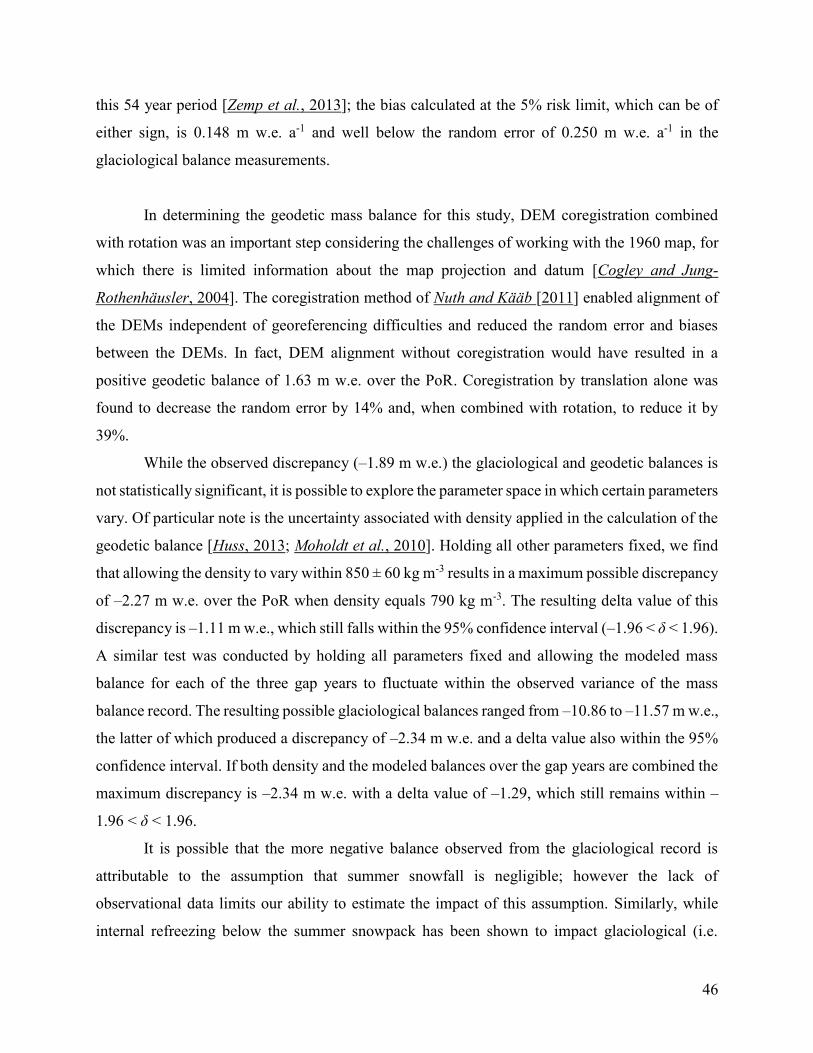
46
this 54 year period [Zemp et al., 2013]; the bias calculated at the 5% risk limit, which can be of
either sign, is 0.148 m w.e. a-1 and well below the random error of 0.250 m w.e. a-1 in the
glaciological balance measurements.
In determining the geodetic mass balance for this study, DEM coregistration combined
with rotation was an important step considering the challenges of working with the 1960 map, for
which there is limited information about the map projection and datum [Cogley and Jung-
Rothenhäusler, 2004]. The coregistration method of Nuth and Kääb [2011] enabled alignment of
the DEMs independent of georeferencing difficulties and reduced the random error and biases
between the DEMs. In fact, DEM alignment without coregistration would have resulted in a
positive geodetic balance of 1.63 m w.e. over the PoR. Coregistration by translation alone was
found to decrease the random error by 14% and, when combined with rotation, to reduce it by
39%.
While the observed discrepancy (–1.89 m w.e.) the glaciological and geodetic balances is
not statistically significant, it is possible to explore the parameter space in which certain parameters
vary. Of particular note is the uncertainty associated with density applied in the calculation of the
geodetic balance [Huss, 2013; Moholdt et al., 2010]. Holding all other parameters fixed, we find
that allowing the density to vary within 850 ± 60 kg m-3 results in a maximum possible discrepancy
of –2.27 m w.e. over the PoR when density equals 790 kg m-3. The resulting delta value of this
discrepancy is –1.11 m w.e., which still falls within the 95% confidence interval (–1.96 < δ < 1.96).
A similar test was conducted by holding all parameters fixed and allowing the modeled mass
balance for each of the three gap years to fluctuate within the observed variance of the mass
balance record. The resulting possible glaciological balances ranged from –10.86 to –11.57 m w.e.,
the latter of which produced a discrepancy of –2.34 m w.e. and a delta value also within the 95%
confidence interval. If both density and the modeled balances over the gap years are combined the
maximum discrepancy is –2.34 m w.e. with a delta value of –1.29, which still remains within –
1.96 < δ < 1.96.
It is possible that the more negative balance observed from the glaciological record is
attributable to the assumption that summer snowfall is negligible; however the lack of
observational data limits our ability to estimate the impact of this assumption. Similarly, while
internal refreezing below the summer snowpack has been shown to impact glaciological (i.e.

47
summer mass balance) and geodetic measurements in other studies (e.g. [Bolch et al., 2013; Huss,
2013] we are unable to treat it quantitatively. Another possible explanation for the more negative
glaciological balance is the missed contribution of mass from superimposed ice originating from
snowmelt off nunataks. In theory superimposed ice, recognized as such, does not impact mass
balance measurements because it is a redistribution of mass within the system. However, snow
originating on nunataks, which is not included in the mass balance calculation, regularly melts and
runs off during the summer months and could refreeze in the accumulation area if the nunatak is
above the ELA, or may freeze as superimposed ice. At present, nunataks comprise 6% of the White
Glacier basin above 1000 m a.s.l. (the approximate average ELA) and including their area in the
glacier hypsometry and subsequent mass balance calculations would only lead to a small increase
(<1%) in the calculated balance. However, as nunataks expand with increasing melt, as we
observed by an increase in the overall nunatak area by 2% from comparison of the White Glacier
1:10,000 maps by Haumann and Honegger [1964] and Thomson and Copland [2016], this
proposed effect may impact mass balance measurements in future years.
3.8 CONCLUSIONS
Reanalysis of the White Glacier mass balance record from 1960-2014 indicates that, in
comparison to the observed geodetic balance, the glaciological method successfully captures the
long-term mass change and does not require correction or calibration. This finding suggests that
the assumptions made in the glaciological method, including that summer accumulation is
negligible at White Glacier, are reasonable for the PoR. One of the more significant findings of
this study was the importance of employing the coregistration techniques of Nuth and Kääb [2011],
and in this case DEM rotation as well, before calculating the geodetic balance. Indeed, failure to
do so would have resulted in a positive geodetic balance over the 54 year period of record, as
opposed to the measured -9.61 m w.e. loss. Homogenization of the glaciological record by
conversion to conventional balances reduced the discrepancy with the geodetic balance by
approximately 0.5 m w.e. More detailed analysis of the individual roles of glacier retreat and
thinning suggests that glacier thinning impacts calculated mass balance to a lesser extent than
glacier retreat, such that loss of significantly negative mass balance regions presents a buffering
effect under the negative mass balance conditions. Corrections applied to address processes that

48
define the generic difference between the glaciological and geodetic balances (i.e. internal and
basal ablation) were found to increase the difference. This may suggest that the surface mass
balance is a reasonable approximation to the total (climatic–basal) mass balance for land-
terminating glaciers in the CAA, which is perhaps not surprising considering the short summer
season at high latitudes during which internal and basal melt might occur.

49
Previous WGMS published version Recommended mass balance series Year Stakes
stakes
Bref ELAref AARref Bcon ELAcon AARcon 1960 71 -408 1261 0.40 -425 1265 0.37 1960 71 -408 1261 0.40 -425 1265 0.37 1961 85 17 931 0.74 19 933 0.74 1962 115 -781 1371 0.20 -782 1373 0.20 1963 80 -155 1172 0.50 -160 1165 0.51 1964 31 349 481 0.91 358 492 0.91 1965 28 -12 886 0.77 -4 889 0.77 1966 51 -25 996 0.69 -13 984 0.70 1967 29 119 828 0.80 137 820 0.81 1968 50 -408 1226 0.44 -405 1222 0.44 1969 76 72 908 0.75 82 905 0.75 1970 68 -4 953 0.73 -9 964 0.72 1971 51 -183 1107 0.60 -194 1114 0.58 1972 91 118 659 0.85 116 672 0.86 1973 49 191 746 0.82 195 761 0.82 1974 48 -44 997 0.69 -48 999 0.68 1975 63 251 800 0.81 250 812 0.81 1976 65 114 832 0.80 120 837 0.80 1977 76 -370 1093 0.60 -388 1117 0.58 1978 23 -131 1018 0.67 -144 1037 0.66 1979 63 -87 1011 0.69 -89 1025 0.66 - - - - - - - 1983 26 -76 980 0.71 -98 991 0.70 1984 27 -44 1009 0.69 -67 1026 0.66 1985 28 1 897 0.76 0 854 0.78 1986 33 -242 1072 0.63 -283 1089 0.61 1987 31 -595 1444 0.10 -626 1442 0.10 1988 25 141 470 0.91 144 457 0.92 1989 31 40 511 0.91 38 505 0.91 1990 27 -431 1395 0.17 -457 1405 0.13 1991 27 -160 1168 0.51 -183 1188 0.47 1992 23 -274 1387 0.21 -286 1396 0.17 1993 23 -423 1376 0.21 -444 1385 0.17 1994 24 -276 1328 0.29 -284 1348 0.25 1995 29 -347 1199 0.47 -381 1222 0.44 1996 32 50 759 0.83 44 754 0.82 1997 45 -38 1055 0.66 -43 1048 0.66 1998 46 -201 1061 0.66 -212 1053 0.64 1999 44 -471 1249 0.41 -484 1247 0.41 2000 51 -405 1299 0.33 -416 1292 0.33 2001 55 -151 1167 0.51 -156 1156 0.51 2002 52 32 848 0.80 27 847 0.80 2003 46 -106 1120 0.58 -114 1112 0.58 2004 55 37 921 0.75 29 918 0.75 2005 33 -612 1291 0.33 -616 1278 0.33 2006 46 -93 1097 0.61 -100 1085 0.61 2007 35 -817 1347 0.25 -843 1347 0.25 2008 43 -806 1397 0.17 -823 1406 0.14 2009 41 -586 1338 0.25 -630 1355 0.21 2010 38 -194 1141 0.55 -216 1156 0.51 2011 28 -987 1428 0.13 -1012 1440 0.11 2012 39 -951 1442 0.10 -974 1458 0.09 2013 28 45 858 0.80 73 857 0.78 2014 39 - - - -417 1329 0.25
Table 3.1: Surface mass balance values and attributes calculated using the reference (ref) and
conventional (con) hypsometry matrices, which are recommended as an update to the previous
WGMS published versions. Mass balance (B) is provided in mm w.e., ELA is the equilibrium
line altitude in meters, and AAR refers to the accumulation area ratio.
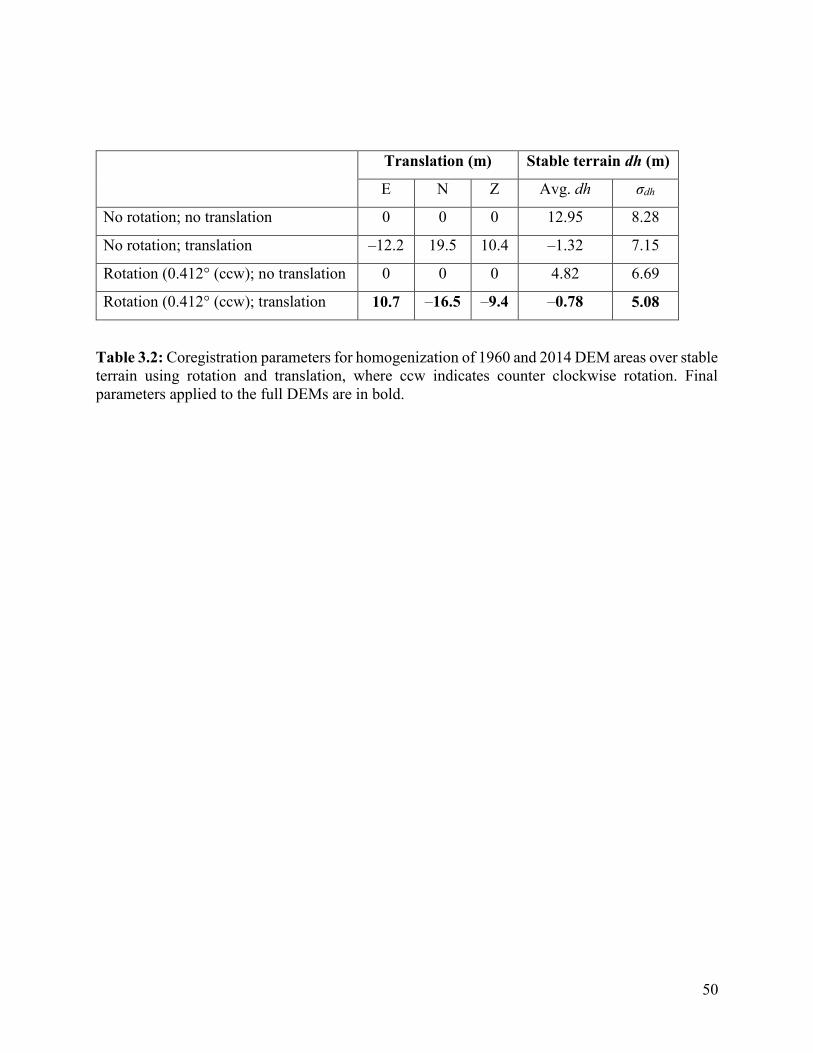
50
Translation (m) Stable terrain dh (m)
E N Z Avg. dh σdh
No rotation; no translation 0 0 0 12.95 8.28
No rotation; translation –12.2 19.5 10.4 –1.32 7.15
Rotation (0.412° (ccw); no translation 0 0 0 4.82 6.69
Rotation (0.412° (ccw); translation 10.7 –16.5 –9.4 –0.78 5.08
Table 3.2: Coregistration parameters for homogenization of 1960 and 2014 DEM areas over stable
terrain using rotation and translation, where ccw indicates counter clockwise rotation. Final
parameters applied to the full DEMs are in bold.
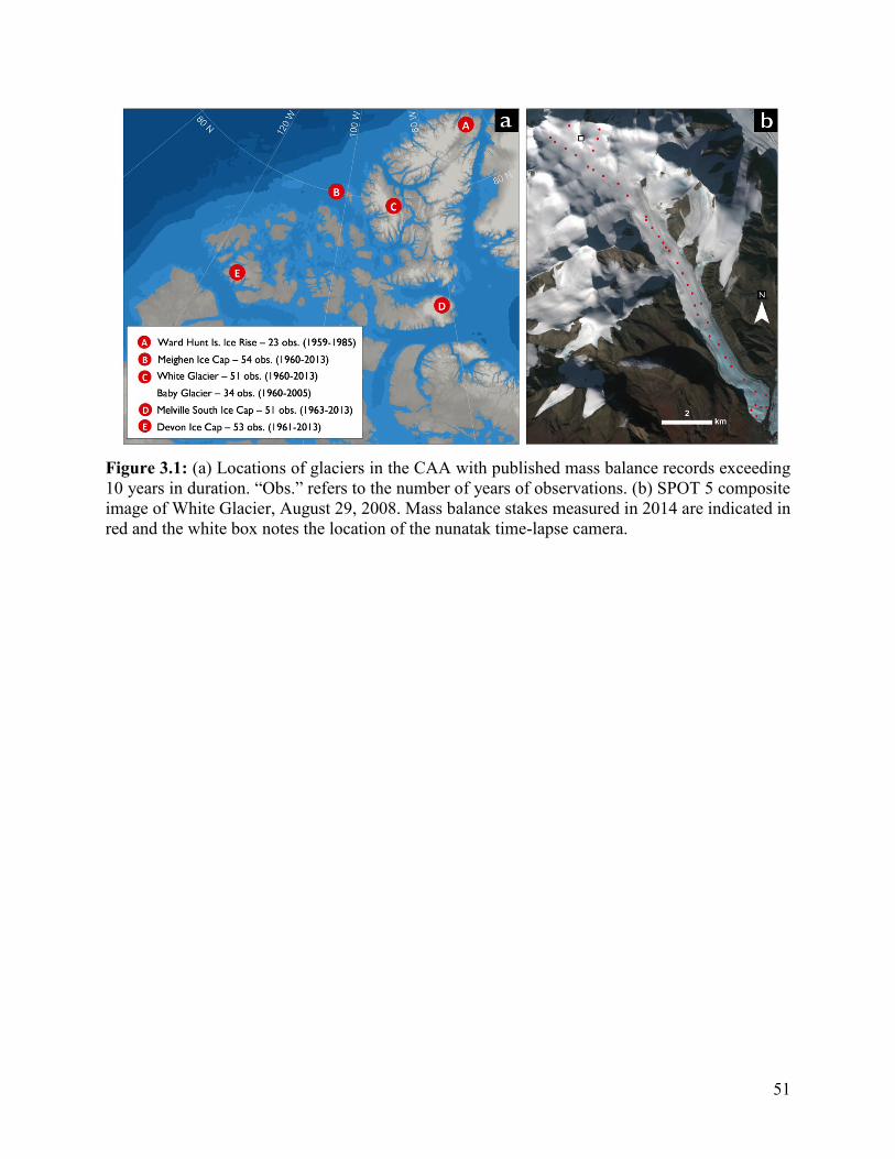
51
Figure 3.1: (a) Locations of glaciers in the CAA with published mass balance records exceeding
10 years in duration. “Obs.” refers to the number of years of observations. (b) SPOT 5 composite
image of White Glacier, August 29, 2008. Mass balance stakes measured in 2014 are indicated in
red and the white box notes the location of the nunatak time-lapse camera.

52
Figure 3.2: (a) The 55 year record of glaciological mass balance (B) with pentadal averages and
standard errors; (b) Equilibrium line altitudes (ELA); (c) Accumulation area ratios (AAR); and (d)
number of mass balance stakes in network.
53
Figure 3.3: (a) Average change in elevation (dh) between 1960 and 2014 observed in each 25 m
hypsometric band (1960 hypsometry and extent shown). The upper right legend refers to elevation
changes over ice, while the lower left legend indicates elevation differences over stable terrain
following the DEM coregistration. The position of the Thompson Glacier terminus as of 2014 is
illustrated in the lower right. (b) White Glacier hypsometry (1960; grey bars) and observed
elevation changes (blue line) over PoR for 100 m elevation bands.

54
Figure 3.4: (a) Stake mass balances for 1960-2014 tending from blue to orange colours over the
PoR. The overlying black line indicates the average linear mass balance gradient. (b) Progression
of the decadal mass balance gradients from 1960-2014, ending with the 2010-2014 pentadal
gradient. Mass balance gradients are in m w.e. km-1.

55
Figure 3.5: Uncorrected and corrected balances from (a) the glaciological method and (b) the
geodetic method. A breakdown of the corrections applied to each method to homogenize the
balances is shown as inset graphs.

56
Figure 3.6: (a) Difference (dB) between the reference (measured) and conventional (modelled
based on a linear change in hypsometry) glaciological balances from 1960 to 2014. (b) Cumulative
balances over the 55-year period with the cumulative difference (dB) plotted above.

57
CHAPTER 4: OBSERVATIONS OF MULTI-DECADAL VELOCITY FLUCTUATIONS
AND MECHANISMS DRIVING LONG-TERM SLOWDOWN
4.1. ARTICLE 3 SUMMARY AND ATTESTATION
Annual and seasonal surface velocities measured continuously from 1960-1970 at White
Glacier provide the most comprehensive historical record of ice dynamics in the Canadian Arctic.
Comparison with dual-frequency GPS-derived velocity data spanning 2012-2016 reveals a general
trend of decreasing ice motion of 10–45%, particularly towards the glacier terminus. However, an
observed increase in summer velocities at high elevations suggests that increased surface-melt and
delivery of this water to the glacier bed through moulins has initiated basal sliding in a zone that
was not subject to significant melt or sliding in earlier decades. The long-term decrease in ice
motion in the lower ablation area of the glacier can be explained by both decreases in internal
deformation driven by reductions in ice thickness of ~15-20 m since the 1960s, and by reduced
basal motion. Despite the long-term slowdown, comparison with theoretical balance velocities
indicates that the flow regime of White Glacier over the period of record is unsustainable with the
current climate.
This study was conducted by Laura Thomson with contributions from Luke Copland. Laura
Thomson was responsible for the compilation of historic data [Iken, 1974; Müller and Iken, 1973]
and the collection, post-processing, analysis, and interpretation of contemporary velocity
measurements. An article based on the following chapter was submitted to Journal of Glaciology
in July 2016 under the title “Long-term reduction in velocities glacier and mechanisms driving
deceleration at polythermal White Glacier, Arctic Canada” and was coauthored by Laura Thomson
and Luke Copland.
4.2 INTRODUCTION
With a change in climate, glaciers can be expected to adjust their extent, thickness, and
flow dynamics to a configuration that is in ‘steady state’ with the new climate [Benn and Evans,
2010]. Glacier mass balance determines the rate of mass transfer required for a glacier to maintain
a geometry in ‘steady state’, such that mass gains at higher elevations are transferred down-glacier
58
at a rate that compensates mass and elevation losses at lower elevations [Nye, 1960]. This rate of
mass movement should define a glacier’s overall velocity structure, although local velocity
patterns are complicated by the variety of mechanisms and processes that define glacier motion.
The mechanics of ice flow are attributable to three primary processes: the deformation of ice
(creep) under gravity [Glen, 1955]; basal motion associated with sliding at the bed [Fowler, 2010];
and basal motion associated with the deformation of the bed [Van der Meer et al., 2003]. For a
given ice thickness, ice deformation rates are strongly related to ice temperature, and basal sliding
and basal sediment deformation are believed to only occur where water is present at the glacier
bed where the ice reaches the pressure melting point.
Under a changing climate, the mechanisms of ice motion might be expected to change due
to changes in ice thickness, ice temperature, and the presence of basal water, but there is currently
considerable uncertainty concerning the direction and magnitude of these changes. For example,
it has been suggested that the speedup of Jakobshavn Isbrae and other outlet glaciers on the western
coast of Greenland are driven by enhanced surface melt at increasingly higher elevations,
prompting increased water pressure at the bed and acceleration of the glacier, thus inducing a
potential positive-feedback cycle whereby dynamic thinning as acceleration draws down high-
elevation ice to lower, warmer elevations [Zwally et al., 2002]. In contrast, other studies suggest a
buffering to this “Zwally effect” in which efficient drainage systems at the glacier bed are able to
develop under high and continuous melt conditions, thus rapidly removing water from the bed and
ultimately reducing the basal water pressures and leading to a slowing of the ice [Schoof, 2010;
Sundal et al., 2011].
There are limited measurements of multi-decadal changes in glacier velocities. One of the
few studies used repeat optical feature-tracking of satellite imagery across several glaciated
regions to indicate that the majority of ice masses have decelerated over time periods spanning up
to 50 years [Heid and Kääb, 2012]. This observed slow-down was mainly attributed to reduced
ice flux as a result of negative mass balance conditions. Other studies of velocity fluctuations of
land-terminating glaciers over several decades show periods of acceleration and deceleration
associated with corresponding increases or decreases in mass balance and ice thickness [Vincent
et al., 2009]. However, since 2000 consistent deceleration appears to be the dominant response,
particularly towards glacier termini [Kaufmann et al., 2015; Tedstone et al., 2015; Waechter et al.,
2015]. In the Canadian Arctic Archipelago (CAA), which is currently responsible for the largest
59
glacier mass losses outside of the ice sheets [Gardner et al., 2013; Harig and Simons, 2016], multi-
decadal changes in ice motion are poorly constrained. Comparison of velocity maps from 2000
and 2011-2015 [Van Wychen et al., 2016] identified that out of 117 large outlet glaciers on
Ellesmere and Axel Heiberg Islands, 7% had slowed by >20 m a-1, 2% had accelerated, and 5%
showed periods of both acceleration and deceleration. No velocity changes were detectable on the
remaining 86% of glaciers, which were generally all slower moving ice masses (<50 m a-1).
Most previous measurements of changes in glacier velocity have focused on large ice caps
and outlet glaciers, meaning that the long-term velocity changes of slow moving ice masses (<100
m a-1) remain relatively unknown. While mountain and valley glaciers comprise a minority of
glacier-covered area in the CAA (e.g. 26% on Axel Heiberg Island), they demonstrate a greater
sensitivity to climate warming both in terms of area change and mass balance [Dowdeswell et al.,
1997; Paul, 2004; Thomson et al., 2011]. One location where it is possible to study detailed
patterns of short- and long-term changes in surface velocities is White Glacier, Axel Heiberg
Island, where Almut Iken conducted her first pioneering studies showing that surface meltwater
was both able to reach the glacier bed and lead to enhanced subglacial water pressures that
facilitated basal sliding [Flowers, 2010; Iken, 1974]. These observations were corroborated by
measurements of englacial ice temperature gradients that supported the existence of a temperate
basal ice zone below the equilibrium line [Blatter, 1987a]. The record of ice velocities at White
Glacier, dating from 1960-1973, is unprecedented in the Canadian Arctic and provides a unique
opportunity to observe changes to the flow regime of polythermal mountain glaciers in the CAA.
This study focuses on a comparison of annual and seasonal velocity observations measured on
White Glacier from 1960-1970 [Iken, 1974; Müller and Iken, 1973] with contemporary
measurements collected between 2012 and 2016 at the same geographic locations. Observed
changes in glacier velocities are investigated in terms of the mechanical processes driving ice
motion and their variability in a changing climate, including changes to glacier mass balance, ice
thickness, and englacial temperatures. While limited observational data is available about the
subglacial conditions at White Glacier, a comparison of observed and theoretical surface velocities
enable us to infer the extent of basal sliding and estimate the dynamic response time of the glacier.

60
4.3 STUDY LOCATION
White Glacier is a 40 km2 mountain glacier measuring ~14 km in length, located on Axel
Heiberg Island in the Canadian Arctic Archipelago (Fig. 4.1). It is characterized by a ~5 km wide
accumulation area which feeds into a narrow (~1 km wide, 9 km long) valley. Elevations range
from 1782 m a.s.l. in accumulation area to 100 m a.s.l. at the glacier terminus. The region
experiences mean annual temperatures of approximately -20°C and annual precipitation ranges
from 58 mm a-1 at sea level (as measured at Eureka, 125 km to the northeast) to 370 mm a-1 at
2120 m a.s.l. [Cogley et al., 1996].
Between 1960 and 1980, White Glacier was the focus of numerous glaciological studies,
including mapping campaigns [Haumann and Honegger, 1964], englacial temperature
measurements [Blatter, 1987a], and velocity surveys at glacier cross-sectional profiles [Iken, 1974;
Müller and Iken, 1973]. Together, these early studies provide important baseline information for
this study, as well as a 55-year mass balance record. Surface mass balance measurements have
continued on a near annual basis since 1959 and the observed balance has become increasingly
negative since 2005 [Cogley et al., 2011a; Thomson et al., 2016], a trend that was not statistically
significant between 1960 and 1991 [Cogley et al., 1996]. There is good agreement between the
cumulative annual surface balance measurements (–213 ± 28 mm w.e. a-1) and the geodetic balance
(–178 ± 16 mm w.e. a-1) calculated over the period 1960-2014. The geodetic data indicates that
thinning has occurred along the length of the glacier below 1400 m a.s.l. since 1960, with losses
exceeding 50 m near the terminus.
The historic (1960-70) and recent (2012-16) velocity measurements were collected at three
profiles located 8.5 km, 5.5 km, and 3.2 km from the glacier terminus (Figure 4.1). The upper
profile (historically referred to as ‘Moraine Profile’) is at 870 m a.s.l. and was located near the
mean equilibrium line observed during the 1960s, while the middle (‘Wind Profile’, 580 m a.s.l.)
and lower (‘Anniversary Profile’, 370 m a.s.l.) profiles are well within the ablation zone since the
onset of measurements at White Glacier. The average equilibrium line altitude (ELA) at the time
of early velocity observations (1960-70) was 990 ± 160 m a.s.l. and located approximately 2 km
up-glacier of the upper profile, but has since risen to 1270 ± 190 m a.s.l. in the last decade (2005-
2015), which equates to approximately 3.5 km up-glacier [Thomson et al., 2016].

61
4.4 METHODS
4.4.1 Velocity observations 1960-1970
Between 1960 and 1968 surveys of annual (va), winter (vw), and summer (vs) velocities
were compiled in Müller and Iken [1973], along with calculations of the mean increase in vs over
va (Δv), melt season duration (s), movement increment during the melt season (Δd), and ablation
(a). Glacier velocities were observed at the upper and lower profiles from repeat stake positions
measured by theodolite surveys of baseline cairns setup along the margins of the glacier [Müller
and Iken, 1973]. These velocity measurements motivated later detailed studies of daily to seasonal
velocity fluctuations by Almut Iken from 1968-1970 as part of her PhD dissertation [Iken, 1974];
this study therefore extends beyond the Müller and Iken [1973] dataset for the upper and lower
profiles by incorporating the velocity data recorded at the middle profile by Iken [1974].
The survey timing at the onset and end of each melt season enabled the calculation of mean
annual and seasonal glacier velocities, with va being defined as the total displacement observed
over one winter season and the following summer melt season (e.g. late-summer 1960 to late-
summer 1961). Velocity errors were calculated from “repeated and 180° reversed readings from
the two ends of a base line” and range from 0.01 to 1.48 cm d-1 [Müller and Iken, 1973]. For each
station, the duration of the melt period (s) was defined by the number of days for which the 5-day
mean daily temperatures surpassed 0°C. These measurements were collected using thermographs
and recorders maintained by members of the research expedition at each of the three stations
[Müller, 1963]. Ablation at each profile was approximated from the mean annual ablation
measured at 5-10 stakes installed across the profile. When in situ observations of ablation or
temperature (for the calculation of s) were not available, estimates were made by interpolation
between the highest and lowest observation sites, or in a few cases extrapolated from climate data
at the Eureka weather station on Ellesmere Island, 125 km northeast of White Glacier (Fig. 4.1a;
see Environment Canada Archive: http://climate.weather.gc.ca/). The errors in s and a (Table 4.1)
consequently reflect the uncertainties associated with extrapolated climate and ablation data. The
applicability of Eureka climate data for conditions at White Glacier in the early studies (1960-70)
is currently unknown, although comparison s derived from summer temperatures at Eureka and
temperatures recorded at an automatic weather station located at the White Glacier terminus from
62
2012 to 2015 indicate that the average difference in mean daily temperatures is <1°C and
maximum residuals do not exceed 5°C (Figure 4.2).
4.4.2 Velocity observations 2012-2016
In 2012, velocity measurements were re-initiated on White Glacier with three Trimble R7
dual-frequency GPS (dGPS) units that were installed at the middle profile in April 2012, at the
upper profile in April 2013, and at the lower profile in July 2013. The dGPS antennae were
mounted on steel poles drilled ~3.5 m into the ice and powered using 50-75 amp hour 12 V batteries
connected to 20 W solar panels. In 2012 the middle dGPS was initially configured to collect
positions every 15 s for 1 hour between 12h00 and 13h00 local time daily, in an effort to prolong
the operating period into the winter months. However, starting in spring 2013 all of the dGPS units
were operated continuously every spring/summer with a 15 s sampling frequency. Post-processing
of dual-frequency GPS data utilized the Precise Point Positioning (PPP) tool provided by Natural
Resources Canada (http://webapp.geod.nrcan.gc.ca/geod/tools-outils/ppp.php), in which the
signal timing between ground stations and receiving satellites, alongside well-constrained satellite
orbital positions, are used to generate baselines for trilateration and positioning. PPP analysis was
conducted using the precise satellite orbits, which are released ~10 days after data acquisition. This
provides three-dimensional (x, y, z) accuracies of approximately ± 2 cm for an observation period
of 1 hour. Appendix 3 provides the daily station coordinates through the duration of this study.
For comparison with the Müller and Iken [1973] and Iken [1974] datasets, it was first
necessary to define the span of the melt season (s) within which vs would be calculated, and the
final day of the melt period that defines the start of the vw and va sample period. As in the earlier
studies, s was defined as the period in which the 5-day mean daily temperature surpassed 0°C.
Shielded HOBO-U23 temperature/relative humidity loggers mounted on poles 1-3 m above the ice
at each dGPS station were used to calculate s, and data gaps were filled by modelled temperatures
using daily temperature lapse-rates derived from two automatic weather stations (AWS) at the
glacier terminus and an upper nunatak (Figure 4.1). Annual ablation (a) was modelled for each
station using the annual mass balance gradient determined from stake measurements along the
glacier centreline. The goodness of fit of the polynomial (n=3) expression of mass balance gradient
that is used to calculate glacier-wide surface mass balance shows an R2 greater than 0.9 for >90%
of the 55 years with observations, and a fit greater than 0.95 for >65% of the record. The mean

63
summer velocity (vs) is determined from displacement between the daily mean positions of the
first and last days of s, divided by s. Errors in dGPS derived velocities are based on a calculation
of the RMSE incorporating the standard deviation of the daily positions divided by the duration of
s.
4.4.3 Surface elevations
The 1:10,000 map of White Glacier by Haumann and Honegger [1964] was used as the
primary source of ice surface elevations between 1960-70. This map, plotted in a local planar
coordinate system with 10 m contours (vertical accuracy considered to be 5 m) was created using
a combination of field-based surveying and photogrammetry methods. A summary of the mapping
techniques for Haumann and Honegger [1964] and associated references are provided in the World
Glacier Monitoring Service’s Fluctuations of Glaciers Maps data archive
(http://wgms.ch/products_fog_maps/). A digital elevation model derived from this map was used
to extract point elevations along the cross-sectional velocity profiles [Thomson and Copland,
2016]. Contemporary surface elevations, based on measurements made in 2014, were derived
from kinematic dGPS measurements collected with a Trimble R7 system mounted on a skidoo and
post-processed with the same online PPP tool as the aforementioned dGPS stations. A 1:10,000
map of White Glacier produced using >400 oblique air photos and Structure from Motion
photogrammetry methods supported determination of elevations near the glacier margins where
dGPS measurements were not possible [Thomson and Copland, 2016]. This map, with a 5 m
vertical accuracy, was also valuable in assessing the amplitude and spatial variability of ice
thinning along the trunk of White Glacier. The 1960 and 2014 DEMs were used to derive glacier
surface slope at each of the three velocity profiles over an along-glacier distance of 2 km (Figure
4.3).
4.4.4 Ice thickness
Cross-sectional ice depth profiles for the three stations were collected in 2014 using a 10
MHz ice penetrating radar system equipped with GPS, as described by Mingo and Flowers [2010].
Assuming a radar wave speed in ice of 1.68 x 10⁸ m s-1, the glacier bed was clearly identifiable at
the lower and middle profiles with an estimated vertical error of <10 m [Wilson, 2012]. At the
upper profile, challenges in interpreting radar returns due to steep rock walls adjacent to the profile
64
resulted in only a single successful measurement of ice thickness, located near the glacier
centreline at the site of the dGPS station. A polynomial regression through the observations was
used to estimate the glacier bed in regions where surface conditions restricted radar measurements
(primarily close to the glacier margins). A parabolic curve best described the measured basal
profiles at the lower and middle sites, with R2 values exceeding 0.9. It was assumed that the bed
profile at the upper profile exhibited a similar parabolic profile to the two lower stations, so the
cross-sectional area of this profile was estimated by fitting a polynomial (n=2) regression through
the single measured ice thickness near the glacier centre and 0 m ice thickness at the glacier
margins (Figure 4.4). The results of the ice radar measurements show reasonable agreement (± 50
m) with early seismic and gravity-based observations of ice thickness conducted in 1961-1962
[Müller, 1963].
Given the superior accuracy of ice surface elevation measurements, changes in ice
thickness were derived from changes in surface height between 1960-70 and 2014 (described
above), rather than comparison of present ice thickness measurements with historic gravity and
seismic observations collected between 1970-1980 [Müller, 1963]. This approach assumes that
basal erosion processes are negligible.
4.5 RESULTS
Annual, winter and summer glacier velocities were calculated for 2012-2016 at the upper,
middle, and lower profiles following the criteria of Müller and Iken [1973] and are shown with the
1960-70 measurements in Figure 4.5. Comparing the historic and contemporary observations,
mean annual velocities decreased at the middle profile from 10.53 cm d-1 to 7.31 cm d-1 (down
31%) and from 8.64 cm d-1 to 5.40 cm d-1 (down 38%) at the lower profile. Mean annual velocities
at the upper station do not show a statistically significant change within their combined errors
(0.82 cm d-1). Mean winter velocities showed a similar trend to the annual velocities with decreases
of 31% (9.62 cm d-1 to 6.72 cm d-1) and 45% (8.08 cm d-1 to 4.45 cm d-1) at the middle and lower
profiles, respectively, and a smaller decrease at the upper profile (3.5%) that is not statistically
significant. The summer patterns are somewhat different; the middle and lower sites exhibited
decreased mean summer velocities by 12% (11.73 cm d-1 to 10.38 cm d-1) and 35% (11.97 cm d-1
to 7.75 cm d-1), respectively, but the upper station exhibited a 12% increase (11.49 cm d-1 to 13.37
65
cm d-1) in mean summer velocity since 1960-70. The detailed velocity time series, including
information on the length of the summer period (s), ablation (a), and associated errors are given in
Table 4.1, which builds upon the record presented in Müller and Iken [1973]. At the upper and
lower profiles, where the historic record of measurements spans 10 years, we find that the percent
contribution of summer motion to annual velocity has increased from 2% to 8% at the upper profile
over the period of record, and from 8% to 15% at the lower profile. We also find that the difference
between winter and annual velocities has increased. In the 1960s, winter velocities were 2% and
8% slower than annual velocities at the upper and lower profiles, respectively, whereas presently
they are 6% and 14% slower.
The longitudinal pattern of ice velocities has also changed from the 1960-70 observations
of Müller and Iken [1973], who observed that va decreased from the upper to middle profiles and
then showed a slight increase to the lower profile, after which the velocity declined steeply towards
the terminus. Our new results indicate a continuous decrease in annual velocity from the upper
profile towards the terminus, with no increase near the lower profile.
The average duration of the summer melt period (s) has increased across the glacier
between the 1960s and today, with the largest change at the upper profile where melt conditions
prevail for 18 days longer per year (Figure 4.6). This corresponds to a 53% increase in melt at the
upper profile in recent years (2011-2015) in comparison to the mean ablation observed from 1960-
70. The increase in s is not as large at the lower profile, only 15 days longer than the 1960-70
average of 65 days, although the increase in ablation is greater than at the upper station with a 73%
increase in melt being observed since the observations of Müller and Iken [1973].
4.6 DISCUSSION
To investigate the potential causes of the observed long-term slowdown in the lower parts
of White Glacier, and lack thereof at the upper profile, we consider how the primary influences on
glacier motion may have changed over time, including internal deformation, basal motion, and
surface mass balance. Additionally, we assess how changes in ice thickness, duration of the melt
period, ablation, and potential changes in englacial temperatures have impacted the processes
controlling ice velocities.
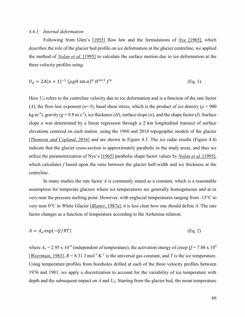
66
4.6.1 Internal deformation
Following from Glen’s [1955] flow law and the formulations of Nye [1965], which
describes the role of the glacier bed profile on ice deformation at the glacier centreline, we applied
the method of Nolan et al. [1995] to calculate the surface motion due to ice deformation at the
three velocity profiles using:
𝑈𝑑 = 2𝐴(𝑛 + 1)−1 (𝜌𝑔𝐻 sin 𝛼)𝑛 𝐻𝑛+1 𝑓𝑛 (Eq. 1).
Here Ud refers to the centreline velocity due to ice deformation and is a function of the rate factor
(A), the flow-law exponent (n=3), basal shear stress, which is the product of ice density (ρ = 900
kg m-3), gravity (g = 9.8 m s-2), ice thickness (H), surface slope (α), and the shape factor (f). Surface
slope α was determined by a linear regression through a 2 km longitudinal transect of surface
elevations centered on each station using the 1960 and 2014 topographic models of the glacier
[Thomson and Copland, 2016] and are shown in Figure 4.3. The ice radar results (Figure 4.4)
indicate that the glacier cross-section is approximately parabolic in the study areas, and thus we
utilize the parameterization of Nye’s [1965] parabolic shape factor values by Nolan et al. [1995],
which calculates f based upon the ratio between the glacier half-width and ice thickness at the
centreline.
In many studies the rate factor A is commonly stated as a constant, which is a reasonable
assumption for temperate glaciers where ice temperatures are generally homogeneous and at or
very near the pressure melting point. However, with englacial temperatures ranging from -15°C to
very near 0°C in White Glacier [Blatter, 1987a], it is less clear how one should define A. The rate
factor changes as a function of temperature according to the Arrhenius relation:
𝐴 = 𝐴𝑜 exp(−𝑄 𝑅𝑇⁄ ) (Eq. 2)
where Ao = 2.95 x 10⁻⁹ (independent of temperature), the activation energy of creep Q = 7.88 x 10⁴
[Weertman, 1983], R = 8.31 J mol-1 K-1 is the universal gas constant, and T is the ice temperature.
Using temperature profiles from boreholes drilled at each of the three velocity profiles between
1976 and 1981, we apply a discretization to account for the variability of ice temperature with
depth and the subsequent impact on A and Ud. Starting from the glacier bed, the mean temperature

67
of 50 m thick segments was calculated for the upper, middle, and lower profiles using englacial
temperature profiles from the boreholes ‘3/81’, ‘4/80’, and ‘1/76’ of Blatter [1987a], respectively
(Figure 4.7a-c). It should be noted that the borehole at the upper station was roughly 100 m short
of the glacier bed, so a linear regression through the lower portion of the profile was used to
estimate the temperatures between the deepest drill depth of 260 m and the bed. From the mean
temperature (�̅�) of each 50 m layer, A was calculated using Eq. 2 and the resulting velocity of each
layer attributable to ice deformation (Ud) was determined from Eq. 1. The sum of Ud values from
each layer thus provides the expected surface velocity attributable to ice deformation at the
centreline (Figure 4.7d-f).
As Eq. 1 indicates, decreases in ice thickness H induce exponential decreases in Ud. For
each station, contemporary ice thickness measurements were determined using the radar methods
and elevation data described in Section 4.4.4. Changes in ice thickness (dH) between 1960 and
2014 at the three stations were: dHupper = -23 m, dHmiddle = -19.5 m, and dHlower = -19 m. The
slightly smaller ice thinning at the middle and lower stations is likely attributable to shadowing
effects at these sites, where the glacier is narrower and confined by steep valley walls. It is also
possible that dynamic thinning is occurring due to flux-divergence at the upper station, notably the
only station that did not demonstrate a statistically significant decrease in va between the 1960s
and present day.
Arguments exist that support both increases and decreases in englacial temperatures under
a warming climate and thinning glacier, with the outcome depending on the dominant processes
taking place [Wilson and Flowers, 2013]. For example, heat delivered from supraglacial
meltwaters to the glacier bed followed by refreezing and the release of latent heat has been
presented as a mechanism for warming and softening the base of the Greenland Ice Sheet [Bell et
al., 2014]. Conversely, for smaller ice masses it has been demonstrated that the loss of ice thickness
reduces englacial strain heating and the capacity for reaching pressure melting point with
decreased overburden pressure [Rippin et al., 2011]. A 3°C warming of annual air temperatures
over the past 60 years has been observed at Eureka station [Lesins et al., 2010], but without
concrete evidence of how englacial temperatures might be changing at White Glacier we
investigate the possibility of both ice warming and cooling in this analysis.
68
Considering the observed changes in ice thickness and potential changes in englacial
temperatures over the past several decades, the above methodology was applied to estimate the
centreline velocity attributable to ice deformation under the following scenarios:
(1) Historic (1960-70) ice thickness (H) and �̅� values (denoted as U1960-70);
(2) Changing ice thickness (dH, 1960 to 2014) and historic �̅� values (UdH);
(3) Changing ice thickness (dH) and a -1°C change to historic �̅� values (UdH -1°C);
(4) Changing ice thickness (dH) and a +1°C change to historic �̅� values (UdH +1°C).
In scenario 4, if the temperature increase led to temperatures >0°C these layers were assigned a
maximum temperature of -0.1°C.
From these scenarios (Figure 4.7d-f), we see that changes in ice thickness alone decrease
deformation rates by 29%, 27%, and 37% respectively at the upper, middle, and lower stations. A
1°C decrease in temperature along the entire temperature profile would theoretically lead to a
further 10-15% decrease in deformation rates at each profile, whereas 1°C of englacial warming
results in ice deformation rates approaching (or exceeding, in the case of the lower profile) those
modeled from 1960-70. The consequences of changing englacial temperatures are most significant
at the lower station, which has the warmest temperature profile. This is likely because deformation
rates are particularly sensitive at temperatures approaching the pressure melting point (~0°C),
where ice deforms at a rate >100 times faster than ice at -20°C [Hambrey, 1994]. We also find that
the proportion of net motion attributable to the deformation of the deepest 50 m of ice increases
from the upper (63%) to the middle (77%) and lower (86%) stations as englacial temperatures near
the bed also increase. Additionally, we find that the modeled depth-averaged velocities, based on
the profiles in Figure 4.7, are very close to the modeled surface velocities (95-96%) and varied by
<1% between stations.
4.6.2 Basal motion
Where the modeled deformation rates fail to meet the observed surface velocities, it is
generally accepted that the residual motion is due to basal sliding or deformation of the bed
[Copland et al., 2003b; Hubbard et al., 1998; Minchew et al., 2015]. We are unable to discriminate
between the relative importance of basal sliding vs. bed deformation processes at the bed of White
Glacier, so from hereon we refer to any motion at the bed simply as basal motion.

69
4.6.2.1 Winter basal motion
The findings of Iken (1974) provided the first evidence that basal motion was able to occur
beneath mostly-cold polythermal Arctic glaciers during the melt season. More recent studies have
indicated that basal motion can also continue through the winter months on polythermal glaciers,
as has been observed at John Evans Glacier on Ellesmere Island [Bingham et al., 2003; Copland
et al., 2003a] and McCall Glacier, Alaska [Rabus and Echelmeyer, 1997].
From the ice deformation model results in scenario 1, with historic ice thickness and
englacial temperature conditions (U1960-70), we find that ice deformation fully accounts for
observed winter velocities at the upper station, but that basal motion is required to explain 47% of
the observed wintertime motion at the middle profile, and 15% at the lower profile (Figure 4.8).
This finding agrees with the suggestion of Blatter [1987a], based on observed ice thicknesses and
temperature profiles, that basal sliding begins just down-glacier of the upper profile where
englacial temperatures closest to the bed transition from approximately -6°C to >-1°C.
For contemporary velocities (2012-16) reductions in H alone (scenario 2; UdH) have led to
a decrease in deformation rates at all stations since 1960-70 (Figure 4.8). Of particular note is the
observed onset of wintertime basal motion that appears to have occurred at the upper profile since
1960-70. This essentially offsets the decrease in ice deformation in that region, such that the overall
changes in vw at the upper profile are negligible. Downstream of the upper profile, the proportion
of wintertime basal motion has decreased since 1960-70, particularly at the lower profile where
internal deformation now accounts for >95% of vw (assuming no changes in englacial
temperatures; UdH = scenario 2). If englacial temperatures have decreased since the observations
of Blatter [1987a], scenario 3 (UdH -1°C) indicates that ice deformation rates would have declined
correspondingly, and increased basal motion is required to reach contemporary winter velocities
at all stations. The converse is true for an increase in englacial temperatures (scenario 4; UdH +1°C),
in which warmer, softer ice will deform more readily.
4.6.2.2 Summer basal motion
The relationship between meltwater delivery to the glacier bed and the resulting magnitude
of basal motion is dependent on the efficiency of the subglacial hydrological network [Flowers,
2015] and its capacity to maintain basal water pressures that reduce friction at the glacier bed
[Bartholomaus et al., 2008]. Glacier speed-up events occur when subglacial water pressures are
70
high and the subglacial hydrological network is unable to efficiently convey water out of the
system, with this behavior observed at both temperate [Iken and Binschadler, 1986; Iken et al.,
1983] and polythermal glaciers [Bingham et al., 2003; Copland et al., 2003b; Iken, 1974]. If the
subglacial hydrological network evolves into a system of large conduits that can efficiently drain
the system and reduce water pressures at the glacier bed, then even high levels of surface melt and
delivery of that water to the bed may not result in glacier speedup, as has been observed and
modeled at locations in Greenland [Schoof, 2010; Sundal et al., 2011] and the Canadian Arctic
[Copland et al., 2003a].
While detailed information about the nature of the subglacial hydrological network at
White Glacier is not available, we can make inferences based on the relationships between ablation
and summer velocities at the upper and lower stations, where the greatest number of historic
observations are available. A weak positive correlation between annual (i.e., summer) ablation and
summer velocity at the upper profile, both historically and recently, suggests that basal motion
occurs in the summer as a result of an inefficient drainage network that supports high basal water
pressures (Figure 4.9). The marked increase in vs at this profile between the 1960s and present day
suggests that over the past half-century the upper profile has shifted flow regimes from being
driven exclusively by ice deformation to a combination of ice deformation and basal motion.
A possible mechanism for the increase in vs at the upper profile relates to the prolonging
of s and a rise of the mean ELA from 1000 to 1270 m a.s.l. (± 160 m) since the 1960-70 mean,
thereby increasing the area of the up-glacier catchment where meltwater can be produced. The
occurrence of many crevasses in this region, some indicative of being the precursors of moulins
given supraglacial streamflow into them, suggest that this meltwater is reaching the bed and
facilitating basal motion in the past decade.
In contrast to the upper profile, a weak negative correlation was found between annual
ablation and vs at the lower profile from 1960-70, suggesting that an efficient subglacial drainage
system was in place over the lower ablation area during this time. Evidence for the presence of a
sustained subglacial drainage system down-glacier of the middle profile includes: (1) the
occurrence of several large active moulins in locations that have remained stable since the mid-
1960s to present; (2) the continued presence of an ice cave that directs a marginal stream beneath
the glacier 1 km down-glacier of the lower profile (first reported in the early 1960s by Maag
[1969]); (3) the recent exposure of very large subglacial and englacial drainage conduits near the

71
glacier terminus following the collapse of the glacier surface between White Glacier and the
adjacent Thompson Glacier in ~2010; (4) the presence of a temperate bed extending from ~200-
700 m a.s.l. [Blatter, 1987a]. Recent observations hint at a possible positive correlation between
vs and ablation at the lower profile, but with only two observations this is not statistically
significant.
4.6.3 Role of mass balance
Over long time periods ice velocities are dictated by glacier mass balance, meaning that
the ice mass passing through a flux gate ought to be equal to the net mass input (i.e. cumulative
mass balance) of the upstream basin [Cuffey and Paterson, 2010]. This theoretical mass turnover
is known as the balance flux, and can be used to calculate the balance velocity when divided by
the cross-sectional area of a flux gate. For each 25 m elevation band (h) on White Glacier, we
calculate the theoretical balance flux (Qb) for each year of the 55 year mass balance record using:
𝑄𝑏(ℎ,𝑡) = ∑ 𝑏(𝑖, 𝑡) 𝑠(𝑖, 𝑡)ℎ0𝑖=ℎ (Eq. 3)
where i ranges from h, a given 25 m elevation band, up to h0, the maximum elevation, b is the
observed elevation band mass balance, s is the area of the elevation band in year t (updated
annually by linear interpolation from 1960-2014 in Thomson et al. [2016], where t is 0 in 1960).
Plotting the annual and decadal mean balance flux profiles illustrates a nearly constant
decline in fluxes towards the present day, with the exception the 1970s (Figure 4.10a). The
elevation at which the balance flux profile intersects Qb=0 indicates the theoretical balance
terminus and is the threshold at which ice flux can be sustained by the cumulative mass balance
conditions upglacier. The decadal mean profiles suggest that the hypsometry of White Glacier
(Figure 4.10b) was dynamically in balance with the climate conditions of the 1970s, the only recent
decade in which Qb=0 at the elevation of the present terminus (~100 m a.s.l.) and for which the
decadal mean glacier wide mass balance was ~0 m w.e.. In all other decades, the elevation of the
balance terminus is well above the present glacier terminus and since 1990 it has risen above the
upper velocity profile (870 m a.s.l), to reach a maximum elevation of 1190 m a.s.l. in 2010-2015.
Observed mass flux (Qobs) through the three velocity profiles, calculated from the product
of the depth averaged velocity (~95% of the observed surface velocity; Section 4.6.1) and the

72
cross-sectional area of the profiles, show that mass fluxes have decreased at all three profiles since
the 1960s (Figure 4.10a). At the upper profile, this decline (-16.4 Mt) is entirely attributable to the
reduction in the cross-sectional area of the profile as a result of ice thinning, while at the middle
and lower profiles both ice thinning and decreased ice velocities have led to the reduced fluxes.
For the main glacier trunk below the middle profile, the cumulative decline in mass flux between
1960 and 2014 has reduced the dynamic replenishment of ice mass by 81.5 Mt below the middle
profile, and 68.2 Mt below the lower profile. These reductions in mass delivery explain only a
small percentage (~2.5%) of the observed mass loss along the glacier terminus below the middle
profile (-3427 Mt) and lower profile (-3043 Mt) based on geodetic mass balance (volume-derived)
mass changes between 1960 and 2014 [Thomson et al., 2016]. This indicates that the observed ~15
m thinning along the main trunk of White Glacier since 1960 is primarily due to down-wasting
(melt), rather than reductions in dynamic mass input. Should ice fluxes along the glacier trunk
continue to decline at a linear rate similar to that observed over 1960-2014, stagnant ice conditions
(Qobs=0) would hypothetically occur within ~80 years at the lower profile, within 110 years at the
middle profile, and within 750 years at the upper profile.
We also find that the dynamic equilibrium line altitude (DELA), defined here as the
elevation at which the maximum flux is expected, is consistently above the ELA that is based on
the mass balance gradient. This observation contradicts general theory [Benn and Evans, 2010;
Cuffey and Paterson, 2010], which suggests that, for a glacier in steady state, maximum mass
turnover (flux) should occur at the ELA. This discrepancy is related to the hypsometry of White
Glacier, which the DELA incorporates, but which the mass balance ELA does not because this is
defined simply as the elevation at which the mass balance gradient intersects b(h)=0. The observed
discrepancy between the DELA and ELA therefore emphasizes the importance of basin geometry
in the stability of glacier response. The hypsometry of the White Glacier basin reaches its
maximum area at elevations of 1300-1500 m a.s.l., meaning that this zone presents an important
threshold. Should the long-term mass balance ELA exceed this elevation range, the glacier will
likely be reduced to a small cirque-type ice mass, which Harrison et al. [2009] characterize as an
‘unstable’ glacier response. Based on the mass balance record the observed ELA has risen by an
average rate of +6 m a-1 over the past 55 years, increasing to a rate of +9 m a-1 over the past 30
years. If the trend persists, then the average ELA will exceed the 1500 m a.s.l. threshold sometime
between ~2040 and 2060.

73
4.7 CONCLUSIONS
Long-term ice velocities are decreasing at White Glacier with the observed decline being
greatest towards the glacier terminus; this result is consistent with studies elsewhere in the Arctic
[Heid and Kääb, 2012]. One exception is the upper station, which showed an increase in summer
velocities suspected to be associated with an increase in meltwater reaching the bed and inducing
basal motion that persists beyond the summer melt period. In agreement with Van Wychen et al.
[2016], we find in our contemporary velocity measurements that winter velocities are ~6-13%
slower than annual velocities, an increase in comparison to earlier velocity measurements [Müller
and Iken, 1973] in which winter velocities were 1-7% lower than annual velocities. Vertical ice
deformation profiles modeled using rate parameters based on historic englacial temperature
measurements [Blatter, 1987a] indicate that ice deformation alone cannot explain contemporary
surface velocities. It is therefore highly likely that basal motion occurs at White Glacier through
the winter, possibly by means of transient water storage at the glacier bed through the winter
months as has been observed at Kennicott Glacier, Alaska [Bartholomaus et al., 2008].
Observed declines in ice flux have not, however, contributed significantly (<2.5%) to
observed mass loss along the glacier trunk from 1960-2014. The observed thinning at low
elevations is therefore primarily associated with high ablation rates and not reduced dynamic
contributions over the past 55 years. It is worthwhile noting that the majority of mass lost between
1960 and 2014 is associated with retreat of the terminus, rather than ice thinning, which acts to
buffer the glacier system by removing ice from low elevations where the largest melt rates occur.
Therefore, with regard to changes in hypsometry, White Glacier is presently exhibiting a stable
response to recent warming. Balance velocities modeled using annual mass balance observations
and glacier hypsometry reveal that the current flow regime is unsustainable and that the observed
mass fluxes through three cross-sectional profiles currently exceed balance fluxes by >200%.
While contemporary ice fluxes appear to be in-sync with mass balance conditions in the 1970s,
possibly suggesting a response time of ~50 years, calculation of response time based on the ratio
between maximum ice thickness (350-400 m) and the average mass balance at the terminus over
the period of record (-2500 mm w.e.) [Benn and Evans, 2010], suggests that White Glacier’s
response time is in fact on the order of 135-155 years. It is expected that ice within the primary
74
glacier trunk below 400 m a.s.l. will become stagnant within the next ~80 years and within the
next 120 years at elevations near 600 m a.s.l. if contemporary deceleration rates continue into the
future.

75
Year va
cm d-1 vw
cm d-1 vs
cm d-1 Δv
% s
d Δd
cm a
cm w.e.
Upper (Moraine) Profile: 870 m a.s.l.; 8.5 km from terminus; 1.3 km wide.
1960-61 10.10 10.10 ± 0.2 10.1 ± 0.2 0.2 ± 4 43 ± 5 0 25 ± 4
61-62 10.53 10.15 ± 0.15 13.00 ± 0.5 28 ± 7 49 ± 4 1.40 ± 0.4 143 ± 11
62-63 9.93 - - - 38 ± 5 - 54 ± 5
63-64 10.25 - - - - - -36
64-65 9.93 - - - - - 45
65-66 9.99 9.89 11.13 ± 0.5 9 ± 5 28 ± 8 0.35 39 ± 9
66-67 10.23 10.20 11.40 ± 0.4 10 ± 5 10 ± 4 0.12 6 ± 2
67-68 10.43 ± 1.0 10.28 11.73 ± 0.2 15 ± 5 44 ± 6 0.64 98 ± 12
68-69 10.75 ± 1.1 10.53 ± 1.03 11.56 ± 1.16 - - - 9 ± 15
69-70 - 11.16 ± 1.05 - - - - 17 ± 15
2011-12 - - - - - - 157 ± 0.9
12-13 - - 12.16 ± 0.13 - 38 - 2 ± 2.6
13-14 10.79 ± 0.10 10.25 ± 0.19 13.93 ± 0.13 39 ± 5 54 2.76 73 ± 0.5
14-15 10.53 ± 0.10 9.70 ± 0.05 14.01 ± 0.10 42 ± 2 68 2.93 128 ± 2.4
15-16 - 9.98 ± 0.08 - - - - -
Middle (Wind) Profile: 580 m a.s.l.; 5.7 km from terminus; 1.2 km wide.
1968-69 10.53 ± 1.05 9.62 ± 0.96 11.73 ± 1.17 - - - 154± 10
2011-12 - - - - - - 208 ± 3
12-13 - 5.72 ± 0.07 10.82 ± 0.05 43 91 2.16 24 ± 1
13-14 6.34 ± 0.04 7.28 ± 0.05 9.32 ± 0.11 - 59 - 126 ± 4
14-15 - - 11.01 ± 0.03 - 92 - 190 ± 9
15-16 - 7.17 ± 0.04 - - 83 - -
Lower (Anniversary) Profile: 370 m a.s.l.; 3.2 km from terminus; 1.0 km wide.
1960-61 8.29 7.78 ± 0.18 12 ± 1.41 49 ± 18 56 ± 4 2.22 ± 0.67 95 ± 5
61-62 8.86 8.28 ± 0.16 11.41 ± 0.67 46 ± 9 69 ± 5 2.47 ± 0.30 245 ± 7
62-63 7.91 7.38 ± 0.01 11.93 ± 1.48 57 ± 21 56 ± 4 2.41 ± 0.84 139 ± 13
63-64 7.89 - - - - - 30 ± 7
64-65 8.53 - - - 68 ± 7 - 122 ± 4
65-66 8.81 8.25 ± 0.01 11.19 ± 0.39 38 ± 5 68 ± 4 2.09 ± 0.07 123 ± 3
66-67 8.84 7.99 ± 0.01 12.82 ± 0.70 58 ± 10 65 ± 6 3.06 ± 0.13 95 ± 8
67-68 8.81 8.24 ± 0.06 11.09 ± 0.10 36 ± 5 74 ± 4 2.15 ± 0.11 201 ± 8
68-69 9.66 ± 0.96 8.60 ± 0.86 12.90 ± 1.29 - - - 127 ± 7
69-70 8.76 ± 0.88 8.08 ± 0.81 12.40 ± 1.24 - - - 106 ± 7
2011-12 - - - - - - 250 ± 4
12-13 - - - - 55 - 46 ± 1
13-14 5.27 ± 0.02 4.62 ± 0.02 7.37 ± 0.02 58 ± 3 92 2.55 ± 0.04 171 ± 6
14-15 5.52 ± 0.02 4.68 ± 0.02 8.12 ± 0.02 86 ± 3 93 3.20 ± 0.04 230 ± 11
15-16 - 4.04 ± 0.05 - - - - -
Table 4.1: Annual and seasonal velocity changes in the ablation area of White Glacier where: va
= mean annual surface velocity; vw = mean winter surface velocity; vs = mean summer surface
velocity; Δv = mean increase of vs over average of preceding and succeeding vw; s = length of
“summer” (melt period); Δd = movement increment during melt period = s(vs -vw); a = ablation.
Observations from 1960-1968 and 1968-1970 originate from Müller and Iken (1973) and Iken
(1974), respectively, while observations from 2012-16 result from dGPS measurements conducted
in this study.

76
Figure 4.1: (a) Location of White Glacier on Axel Heiberg Island (red triangle) and the Eureka
weather station (yellow circle). (b) Map of White Glacier showing the location of 3 cross-sectional
profiles and the location of crevasses (light grey lines) and moulins (blue circles) identified in Iken
(1974) that are still present as of 2014 Field observations suggest a new moulin has formed within
100 m southeast of the upper profile, but it is not confirmed if it is regularly active.

77
Figure 4.2: Comparison of daily mean temperatures observed at the Environment Canada
Eureka weather station and at an automatic weather station (AWS) located at the terminus of
White Glacier in (a) 2012, (b) 2013, and (c) 2014.
c
a
b

78
Figure 4.3: Surface slope profiles in 1960 (a, b, c) and in 2014 (d, e, f) at the upper, middle, and
lower profiles, respectively.

79
Figure 4.4: Cross sectional depth and elevation profiles based on 10 MHz ice penetrating radar
measurements at the (a) upper, (b) middle, and (c) lower velocity profiles.
a
b
c
Upper Profile (870 m a.s.l.)
Middle Profile (580 m a.s.l.)
Lower Profile (370 m a.s.l.)

80
Figure 4.5: Variations in annual, winter, and summer velocities between 1960-70 [Müller and
Iken, 1973] and 2012-2016 (this study) at the (a) upper, (b) middle, and (c) lower velocity profiles.
Summer and winter errors are indicated as vertical lines on the summer and winter velocities.

81
Figure 4.6: Annual ablation (a) derived from mass balance measurements and duration of the
melt period (s) for the: (a) upper, and (b) lower profiles. Negative ablation values indicate that
the profile was in the accumulation area (e.g. in 1963). Missing s values refer to years where
meteorological data was not available for the given profile.
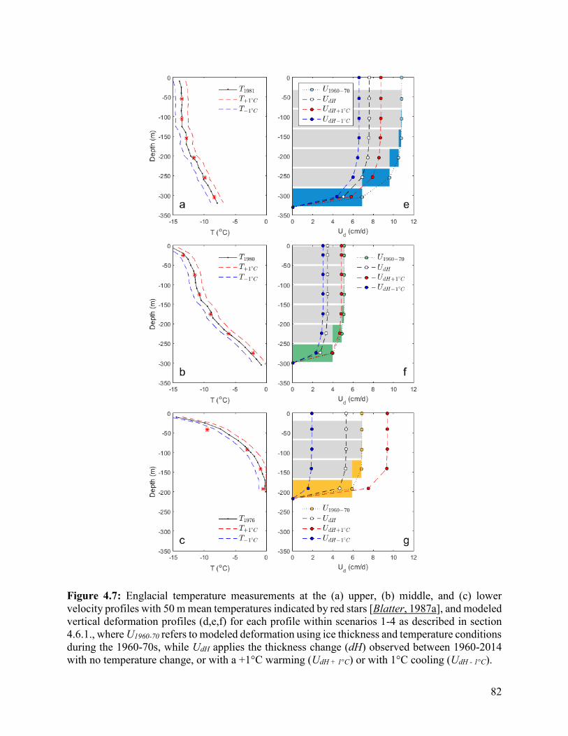
82
Figure 4.7: Englacial temperature measurements at the (a) upper, (b) middle, and (c) lower
velocity profiles with 50 m mean temperatures indicated by red stars [Blatter, 1987a], and modeled
vertical deformation profiles (d,e,f) for each profile within scenarios 1-4 as described in section
4.6.1., where U1960-70 refers to modeled deformation using ice thickness and temperature conditions
during the 1960-70s, while UdH applies the thickness change (dH) observed between 1960-2014
with no temperature change, or with a +1°C warming (UdH + 1°C) or with 1°C cooling (UdH - 1°C).

83
Figure 4.8: Component of winter surface velocity attributable to deformation (hatched pattern)
and basal motion (solid colour) at the (a) upper, (b) middle, and (c) lower velocity profiles for
scenarios 1-4 described in section 4.6.1., where U1960-70 refers to modeled deformation using ice
thickness and temperature conditions during the 1960-70s, while UdH applies the thickness change
(dH) observed between 1960-2014 with no temperature change, or with a +1°C warming (UdH +
1°C) or with 1°C cooling (UdH - 1°C).

84
Figure 4.9: Relationship between annual ablation and summer velocities (vs) at the (a) upper and
(b) lower profiles, and on velocities the following winter (vw) at the (c) upper and (d) lower profiles.

85
Figure 4.10: (a) Annual (grey) and decadal mean (coloured) balance flux (Qb) profiles based upon
the 55-year mass balance record at White Glacier. Also plotted are the observed fluxes (Qobs)
derived from 1960-70 velocities (white triangles) and 2012-16 velocities (red triangles). Coloured
circles and triangles respectively refer to the dynamic ELA where maximum flux occurs, and the
corresponding ELA based on surface mass balance data. (b) Glacier hypsometry in 1960 (black)
based upon Haumann and Honegger [1964] and 2014 (red) from Thomson and Copland [2016b].
86
CHAPTER 5: CONCLUSIONS AND FUTURE WORK
5.1. SUMMARY AND SYNTHESIS
Building upon the rich archive of early glaciological studies at White Glacier, Axel Heiberg
Island, Nunavut, this thesis has: (1) quantified changes to the glacier hypsometry (area-elevation
distribution), mass balance, and ice dynamics since 1960, (2) sought to elucidate the primary
processes driving the observed changes, (3) makes simple predictions about the glacier’s future.
5.1.1 Summary of primary findings
The first requirement of this study was to create an updated map of White Glacier from
which changes in ice thickness and glacier hypsometry could be determined. Using >400 oblique
aerial photographs collected in July 2014, a new digital elevation model (DEM) was created using
Structure from Motion techniques, a method built upon traditional photogrammetry but with the
advantage of automated image correlation analysis [Fonstad et al., 2013]. The outcome of this
work demonstrated that, with careful camera setup, the Structure from Motion method is able to
overcome the challenges of optical remote sensing in low-contrast, snow-covered areas due to the
high resolution of the photographs and their ability to detect of small features at the surface. The
resulting DEM and orthoimage facilitated the production of a new 1:10,000 topographic map of
White Glacier with 5 m vertical accuracy in the style of earlier cartographic works dating back to
1960 [Haumann and Honegger, 1964].
The new map supported the calculation of the glacier’s geodetic mass balance (mass
change determined from ice volume change) and provided an updated glacier hypsometry that
improves the accuracy of contemporary mass balance calculations. A modeled glacier hypsometry
time series was created to support a reanalysis of the mass balance record, from which comparison
of the geodetic and glaciological methods enabled the detection of generic differences and
potential sources of error in the glaciological method [Zemp et al., 2013]. Statistical comparison
of the two approaches revealed that, within error margins, there was no significant difference
between the average annual glaciological mass balance (–213 ± 28 mm w.e. a-1) and geodetic mass
balance (–178 ± 16 mm w.e. a-1) of White Glacier between 1960 and 2014.
87
To determine how ice dynamics have responded to a long-term trend of ice thinning and
increasingly negative mass balance conditions, dual-frequency GPS stations were installed at the
centre of three cross-sectional profiles on White Glacier to continuously monitor ice motion from
2012–2016. These sites were the focus of surface velocity measurements from 1960–1970 [Iken,
1974; Müller and Iken, 1973]. Comparison of annual, winter, and summer velocities indicated
decreasing ice motion of ~10–45%, with biggest reductions towards the glacier terminus.
However, an observed increase in summer velocities at the highest station suggested that increased
surface melt and delivery of this water to the glacier bed through moulins has initiated basal sliding
in a zone that was not subject to this effect in earlier decades. The component of surface velocity
attributable to ice deformation was modeled using Glen’s [1955] flow law applied with site-
specific enhancement factors derived from earlier englacial temperature observations. These
calculations enabled the estimation of historic and contemporary basal sliding velocities for each
station and indicate that for the stations below 600 m a.s.l., basal sliding has diminished while
internal deformation rates have remained constant, or may have increased in response to an
increasing annual air temperature of ~3°C [Lesins et al., 2010]. Comparison of observed fluxes
through cross-sections at the three velocity profiles with balance fluxes modeled from the long-
term mass balance record indicated that the current flow regime of White Glacier is not sustainable.
5.1.2 Synthesis
The combined results provide some insight into the stability of the post-1960 response of
White Glacier since early observations in 1960 which coincided with the onset of contemporary
amplified warming in the Arctic [Screen and Simmonds, 2010]. Foremost, negative mass balance
conditions have continued to increase since the last detailed assessments of the data [Cogley et al.,
2011a; Cogley et al., 1996], with 8 of the 10 most negative mass balance years being observed in
the last 15 years. It has been well established in previous studies that the mass balance of glaciers
in the CAA is primarily attributable (>90%) to summer surface air temperatures, rather than
variability in accumulation [Koerner, 2005; Sharp et al., 2011]. While predictions that
precipitation will increase with diminishing Arctic sea ice [e.g. Kopec et al., 2016] have proven
true in some parts of the northern hemisphere and particularly over Siberia [Cohen and Cherry,
2012; Ghatak, 2012], no statistically significant changes have been observed in the accumulation
area of White Glacier since the 1960s. Similarly, the suggestion that mass balance gradients should
88
steepen, due to the potential shift from continental- to maritime-type climates with decreasing sea
ice [Dyurgerov and Dwyer, 2000], has not been detected either (see Chapter 3, Figure 3.4).
Changes in the elevation and extent of White Glacier, through comparison of the new 2014
1:10,000 map [Thomson and Copland, 2016b] and the original 1960 map [Haumann and
Honegger, 1964], reflect a dominant trend of ice thinning with >20 m of elevation loss having
occurred below 1000 m a.s.l. (see Chapter 3, Figure 3.3), and a retreat of the terminus by ~1 km.
Decreases in hypsometry at higher elevations (1000-1400 m a.s.l.) are also attributable to the
increasing size of nunataks as high elevation ice thins, thereby exposing more of the bedrock
below. Elevation losses along the main trunk of the glacier below ~700 m a.s.l. are primarily due
to increased ablation (>97%) rather than reductions in the dynamic contribution of mass towards
the terminus as the glacier slows down. Although thinning has negative repercussions for glacier
mass balance by shifting more ice to lower, warmer elevations, it was found that the magnitude of
this effect was more than offset by the positive response of glacier retreat, which acts to remove
ice from elevations where the maximum potential for melt occurs. This suggests that the glacier,
in regard to changes in hypsometry, is presently exhibiting a stable response to current warming.
However, if the observed rate of thinning persists into the future and continues to impact higher
elevations, as has been modeled for Yakutat Glacier in southeast Alaska [Trüssel et al., 2015], a
threshold will pass at which the retreat response will no longer have the capacity to offset enhanced
melt at higher elevations.
5.2 KEY CONTRIBUTIONS
This thesis presents several new contributions to Canadian Arctic glaciology by reporting
the first multi-decadal observations of changes to mountain glacier hypsometry and dynamics, and
by demonstrating new methods of analysis that reflect the stability of glacier response.
As demonstrated by the scientific value of the original 1960 1:10,000 map of White Glacier
[Haumann and Honegger, 1964], the new map produced using Structure from Motion techniques
(Chapter 2) contributes an important baseline of the glacier extent and elevation for future research.
In addition to providing an updated hypsometry that improves the accuracy of mass balance
calculations in the future, the new map also presents a record of surface features on the glacier
(e.g. crevasses, surface streams, terminus collapse feature) that reflect the contemporary dynamics

89
and supraglacial hydrological system. The new White Glacier map (2014; Appendix 1), as well as
the entire collection of large-scale Expedition Fiord maps produced in the 1960s, have now been
submitted to the World Glacier Monitoring Service’s ‘Fluctuations of Glaciers – Maps’ digital
archive (www.wgms.ch/products_fog_maps) to ensure that they are properly archived and
accessible in the future.
This thesis also provides the first reanalysis of a high-Arctic glacier mass balance record
in the Canadian Arctic. Through rigorous statistical analysis it confirms, for the first time, that the
fundamental assumptions made in the glaciological method applied at White Glacier (e.g. that
summer accumulation is negligible) are reliable and do not impose any statistically significant
biases into the record spanning 1960-2014. New analysis of the individual roles of glacier retreat
and thinning provided the first evidence that glacier thinning impacts calculated mass balance to a
lesser extent than glacier retreat, such that loss of strongly negative mass balance regions presents
a buffering effect under negative mass balance conditions. However, it is not yet possible to say
whether this response is occurring at other mountain glaciers in the CAA.
Ice velocity measurements presented in this thesis show the first observations of glacier
deceleration in the CAA occurring over the span of more than 50 years. These measurements also
revealed that the contribution of summer movement to annual motion has increased significantly
since the 1960s at all stations. A new method of modeling internal deformation rates, in which the
flow rate parameter was allowed to vary with depth according to englacial temperatures, showed
good agreement at high elevations where historically all ice motion was attributable to creep
processes. It was also discovered that basal motion (by sliding or deformation of the bed) is likely
now occurring at higher elevations where historically surface velocities were entirely explainable
by ice deformation.
The broader impact of this research concerns the provision of in situ observations and
interpretation of glacier-climate interactions in a region where most glacier monitoring is
dominated by large-scale remote sensing endeavors with limited ground-based validation. At
present, the data in this thesis comprise the only contemporary field measurements of a mountain
glacier in the Canadian Arctic despite a majority of CAA glaciers (according to number, rather
than area), and those with the most significant evidence of retreat, being classified as alpine type
[Oerlemans and Fortuin, 1992; Thomson et al., 2011].

90
5.3 FUTURE WORK
This thesis demonstrates the value of long-term glacier monitoring programs and the
scientific opportunity provided by comprehensive and well documented baseline studies.
Therefore, future work at White Glacier should foremost ensure the continuation of the annual
glaciological mass balance measurements and continued submission of this data to the World
Glacier Monitoring Service. As a follow-up to the reanalysis of the mass balance record (Chapter
3), the White Glacier record held at WGMS will be updated to reflect the conventional mass
balance between 1960 and 2014, calculated using a linear interpolation of hypsometry between
those years. Future calculations of glaciological mass balance will use the new 2014 hypsometry
until another topographic survey is conducted. While the assumption that summer accumulation is
negligible holds true following the reanalysis findings presented here, this may not be so in the
future. We have therefore established a new automated snow-depth sounder at the highest mass
balance stake on White Glacier (1480 m a.s.l.) to monitor snowfall patterns through the year.
The intention is to continue monitoring ice velocities on White Glacier at the upper, middle,
and lower profiles, alongside the mass balance measurements, as a means of determining whether
the observed deceleration will persist. An important question is whether this slowdown will occur
at a constant rate, or whether the glacier will behave in a non-linear fashion, which might be
expected given that deformation rates decrease exponentially with decreasing ice thickness [Glen,
1955]. With the observation that the contribution of summer motion to annual velocities has more
than doubled at lower elevations, and quadrupled at the upper station, it is essential to monitor this
behaviour into the future to determine if and when it is no longer appropriate to assume that winter
motion is representative of annual motion in remote sensing studies of ice dynamics.
A new project will begin in the fall of 2016 to investigate the evolution of englacial
temperatures, which in Chapter 4 are shown to have a significant impact on the rate of ice
deformation. This work will repeat early field measurements of englacial temperatures [Blatter,
1987a] in the upper 15-20 m of the glacier and will integrate the historic and contemporary
measurements as boundary conditions into a thermodynamical model of ice temperatures through
time [Wilson and Flowers, 2013]. The goal of this work is to elucidate how englacial temperatures
impact the dynamic processes (including ice deformation, basal motion, and the supra- and
subglacial hydrological networks) of mostly-cold polythermal glaciers, a thermal-state considered
91
to describe the majority of ice masses in the CAA, and what the long-term effects will be on glacier
response.
In closing, this thesis highlights the admirable quality of the early glaciological studies
conducted in the Expedition Fiord region of Axel Heiberg, and demonstrates the scientific
potential that exists for countless more future studies built upon the foundation of research
established there.
92
CHAPTER 6: REFERENCES
Adams, W. P. (1966), Ablation and run-off on the White Glacier. Axel Heiberg Island, Canadian
Arctic Archipelago., Axel Heiberg Island Research Reports, Glaciology, No. 1, pp. 84.
AMAP (2011), Snow, Water, Ice and Permafrost in the Arctic (SWIPA): Climate Change and the
Cryosphere, Oslo, Norway.
Andreassen, L. M., H. Elvehøy, B. Kjøllmoen, and R. V. Engeset (2015), Glaciological and
geodetic mass balance of ten long-term glaciers in Norway, The Cryosphere Discuss.,
9(6), 6581-6626, doi:10.5194/tcd-9-6581-2015.
Andrews, R. H. (1964), Meteorology and heat balance of the ablation area, White Glacier.
Canadian Arctic Archipelago - Summer 1960., Axel Heiberg Island Research Reports,
Meteorology, No.1, 116 pp.
Arnold, K. C. (1981), Ice ablation measured by stakes and terrestrial photogrammetry - a
comparison on the lower part of the White Glacier. Axel Heiberg Island, Canadian Arctic
Archipelago., Axel Heiberg Island Research Reports, Glaciology, No.2, pp. 106.
Bartholomaus, T. C., R. S. Anderson, and S. P. Anderson (2008), Response of glacier basal
motion to transient water storage, Nature Geoscience, 1, 33-37.
Bell, R. E., K. Tinto, I. Das, M. Wolovick, W. Chu, T. T. Creyts, N. Frearson, A. Abdi, and J. D.
Paden (2014), Deformation, warming and softening of Greenland's ice by refreezing
meltwater, Nature Geosci, 7(7), 497-502, doi:10.1038/ngeo2179
Benn, D. I., and D. J. A. Evans (2010), Glaciers and Glaciation, Hodder Education.
Bingham, R. G., P. W. Nienow, M. Sharp, and L. Copland (2006), Hydrology and dynamics of a
polythermal (mostly cold) High Arctic glacier, Earth Surface Processes and Landforms,
31, 1463-1479.
Bingham, R. G., P. W. Nienow, and M. J. Sharp (2003), Intra-annual and intra-seasonal flow
dynamics of a High Arctic polythermal valley glacier, Annals of Glaciology, 37(1), 181-
188, doi:10.3189/172756403781815762.
Blachut, T. J. (1961), Participation of the Photogrammetric Research Section of the N.R.C., in
Preliminary Report of 1959-60, Jacobsen-McGill Arctic Research Expedition to Axel

93
Heiberg Island, Queen Elizabeth Islands, edited by B. S. Müller, pp. 27-33, McGill
University, Montreal.
Blachut, T. J. (1963), Photogrammetric and cartographic results of the Axel Heiberg Island
expedition, Canadian Surveyor, 17(2), 79-80.
Blatter, H. (1987a), On the thermal regime of an Arctic valley glacier: a study of White Glacier,
Axel Heiberg Island, N.W.T., Canada, Journal of Glaciology, 33(114), 200-211.
Blatter, H. (1987b), Stagnant ice at the bed of White Glacier, Axel Heiberg Island, N.W.T.,
Canada, Annals of Glaciology, 9, 35-38.
Bolch, T., L. Sandberg Sørensen, S. B. Simonsen, N. Mölg, H. Machguth, P. Rastner, and F.
Paul (2013), Mass loss of Greenland's glaciers and ice caps 2003–2008 revealed from
ICESat laser altimetry data, Geophysical Research Letters, 40(5), 875-881,
doi:10.1002/grl.50270.
Braithwaite, R. J. (2005), Mass-balance characteristics of arctic glaciers, Annals of Glaciology,
42(1), 225-229, doi:10.3189/172756405781812899.
Braithwaite, R. J., and S. C. B. Raper (2007), Glaciological conditions in seven contrasting
regions estimated with the degree-day model, Annals of Glaciology, 46, 297-302.
Braun, C., D. R. Hardy, and R. S. Bradley (2004a), Mass balance and area change of four High
Arctic plateau ice caps, Geografiska Annaler, 86A, 43-52.
Braun, C., D. R. Hardy, R. S. Bradley, and V. Sahanatien (2004b), Surface mass balance of the
Ward Hunt Ice Rise and Ice Shelf, Ellesmere Island, Nunavut, Canada, Journal of
Geophysical Research, 109(D22110), doi:10.1029/2004JD004560.
Burgess, D. O., M. J. Sharp, D. W. F. Mair, J. A. Dowdeswell, and T. J. Benham (2005), Flow
dynamics and iceberg calving rates of Devon Ice Cap, Nunavut, Canada, Journal of
Glaciology, 51(173), 219-230, doi:10.3189/172756505781829430.
Castner, H. W., and R. Wheate (1979), Re-assessing the role played by shaded relief on
topographic scale maps, The Cartographic Journal, 16(2), 77-85.
Cogley, J. G. (2009), Geodetic and direct mass-balance measurements: comparison and joint
analysis, Annals of Glaciology, 50, 96-100.

94
Cogley, J. G., and W. P. Adams (1998), Mass balance of glaciers other than the ice sheets,
Journal of Glaciology, 44(147), 315-325, doi:10.3189/172756409787769744.
Cogley, J. G., and W. P. Adams (2000), Remote-sensing resources for monitoring glacier
fluctuations on Axel Heiberg Island, Arctic, 53(3), 248-259,
doi:10.3189/172756409787769744.
Cogley, J. G., W. P. Adams, and M. A. Ecclestone (2011a), Half a century of measurements of
glaciers on Axel Heiberg Island, Nunavut, Canada, Arctic, 64(3), 371-375,
doi:10.14430/arctic4127.
Cogley, J. G., W. P. Adams, M. A. Ecclestone, F. Jung-Rothenhäusler, and C. S. Ommanney
(1996), Mass balance of White Glacier, Axel Heiberg Island, N.W.T., 1960-1991,
Journal of Glaciology, 42(142), 548-563.
Cogley, J. G., et al. (2011b), Glossary of Glacier Mass Balance and Related Terms, in IHP-VII
Technical Documents in Hydrology No. 86, IACS Contribution No. 2, edited by
UNESCO-IHP, pp. 114, Paris.
Cogley, J. G., and F. Jung-Rothenhäusler (2002), Digital Elevation Models of Axel Heiberg
Island Glaciers, Rep., pp. 46, Department of Geography, Trent University, Peterborough,
Canada.
Cogley, J. G., and F. Jung-Rothenhäusler (2004), Uncertainty in digital elevation models of Axel
Heiberg Island, Arctic Canada, Arctic, Antarctic, and Alpine Research, 36(2), 249-260.
Cohen, J. L., J. C., Furtado, M. A. Barlow, V. A. Alexeev, and J. E. Cherry (2012), Arctic
warming, increasing snow cover and widespread boreal winter cooling, Environmental
Research Letters, 7(1), 014007.
Copland, L., M. Sharp, and P. W. Nienow (2003a), Links between short-term velocity variations
and the subglacial hydrology of a predominantly cold polythermal glacier, Journal of
Glaciology, 49(166), 337-348.
Copland, L., M. J. Sharp, P. Nienow, and R. G. Bingham (2003b), The distribution of basal
motion beneath a High Arctic polythermal glacier, Journal of Glaciology, 49(166), 407-
414, doi:10.3189/172756503781830511.
Cuffey, K. M., and W. S. B. Paterson (2010), The Physics of Glaciers, Fourth ed., Elsevier,
Amsterdam.

95
Dowdeswell, J. A., et al. (1997), The Mass Balance of Circum-Arctic Glaciers and Recent
Climate Change, Quaternary Research, 48(1), 1-14,
doi:http://dx.doi.org/10.1006/qres.1997.1900.
Dyurgerov, M. B., and J. Dwyer (2000), The steepening of glacier mass balance gradients with
Northern Hemisphere warming, Zeitschrift für Gletscherkunde und Glazialgeologie, 36,
107-118.
Elsberg, D. H., W. D. Harrison, K. A. Echelmeyer, and R. M. Krimmel (2001), Quantifying the
effects of climate and surface change on glacier mass balance, Journal of Glaciology,
47(159), 649-658, doi:10.3189/172756501781831783.
Fisher, D., J. Zheng, D. O. Burgess, C. Zdanowicz, C. Kinnard, M. Sharp, and J. Bourgeois
(2012), Recent melt rates of Canadian arctic ice caps are the highest in four millennia,
Global and Planetary Change, 84-85, 3-7.
Flowers, G. E. (2010), Glacier hydromechanics: early insights and the lasting legacy of three
works by Iken and colleagues, Journal of Glaciology, 56(200), 1069-1078,
doi:10.3189/002214311796406103.
Flowers, G. E. (2015), Modelling water flow under glaciers and ice sheets, Proceedings of the
Royal Society of London A: Mathematical, Physical and Engineering Sciences,
471(2176), doi:10.1098/rspa.2014.0907.
Fonstad, M. A., J. T. Dietrich, B. C. Courville, J. L. Jensen, and P. E. Carbonneau (2013),
Topographic structure from motion: a new development in photogrammetric
measurement, Earth Surface Processes and Landforms, 38(4), 421-430,
doi:10.1002/esp.3366.
Fowler, A. C. (2010), Weertman, Lliboutry and the development of sliding theory, Journal of
Glaciology, 56(200), 965-972.
Furbish, D. J., and J. T. Andrews (1984), The use of hypsometry to indicate long-term stability
and response of valley glaciers to changes in mass transfer, Journal of Glaciology,
30(105), 199-211.
Gardner, A., et al. (2013), A Reconciled Estimate of Glacier Contributions to Sea Level Rise:
2003-2009, Science, 340, 852-857.
96
Gardner, A., G. Moholdt, B. Wouters, G. J. Wolken, D. O. Burgess, M. Sharp, J. G. Cogley, C.
Braun, and C. Labine (2011), Sharply increased mass loss from glaciers and ice caps in
the Canadian Arctic Archipelago, Nature, 473, 357-360.
Gardner, A., and M. Sharp (2007), Influence of the Arctic Circumpolar Vortex on the Mass
Balance of Canadian High Arctic Glaciers, Journal of Climate, 20, 4586-4598,
doi:10.1175/JCLI4268.1.
Ghatak, D., C. Deser, A. Frei, G. Gong, A. Phillips, D. A. Robinson, and J. Stroeve (2012),
Simulated Siberian snow cover response to observed Arctic sea ice loss, 1979–2008,
Journal of Geophysical Research: Atmospheres, 117 (D23108),
doi:10.1029/2012JD018047.
Glen, J. W. (1955), The Creep of Polycrystalline Ice, Proceedings of the Royal Society of London
A: Mathematical, Physical and Engineering Sciences, 228 (1175), 519-538,
doi:10.1098/rspa.1955.0066.
Glenday, P. J. (1989), Mass balance parameterization. White Glacier, Axel Heiberg Island, N.
W. T., 1970-1980., Department of Geography, Trent University, Peterborough, ON,
Canada.
Hambrey, M. (1994), Glacial Environments, Taylor & Francis.
Harig, C., and F. J. Simons (2016), Ice mass loss in Greenland, the Gulf of Alaska, and the
Canadian Archipelago: Seasonal cycles and decadal trends, Geophysical Research
Letters, 43(7), 3150-3159, doi:10.1002/2016GL067759.
Harrison, W. D., L. H. Cox, R. Hock, R. S. March, and E. C. Pettit (2009), Implications for the
dynamic health of a glacier from comparison of conventional and reference-surface
balances, Annals of Glaciology, 50(50), 25-30, doi:10.3189/172756409787769654.
Hattersley-Smith, G., and H. Serson (1970), Mass balance of the Ward Hunt Ice Rise and Ice
Shelf: A 10 year record, Journal of Glaciology, 9 (56), 247-252.
Haumann, D. (1961), Co-ordinates of ground control points determined in 1960, in Preliminary
Report of 1959-60, Jacobsen-McGill Arctic Research Expedition to Axel Heiberg Island,
Queen Elizabeth Islands, edited by B. S. Muller, pp. 35-42, McGill University, Montreal.
Haumann, D. (1963), Surveying glaciers in Axel Heiberg Island, Canadian Surveyor, 17(2), 81-
93.

97
Haumann, D., and D. Honegger (1964), White Glacier, Axel Heiberg Island, Canadian Arctic
Archipelago, 1:10,000, McGill University, Photogrammetric Research Section, National
Research Council of Canada.
Havens, J. M., F. Müller, and G. C. Wilmot (1965), Comparative meteorological survey and a
short-term heat balance study of the White Glacier. Canadian Arctic Archipelago -
Summer 1962, Axel Heiberg Island Research Reports, Meteorology, No.4, 76.
Heid, T., and A. Kääb (2012), Repeat optical satellite images reveal widespread and long term
decrease in land-terminating glacier speeds, The Cryosphere, 6, 467-479.
Hember, R. A., J. G. Cogley, and M. A. Ecclestone (2003), Volume balance of White Glacier
terminus, Axel Heiberg Island, Nunavut, 1961-2003, in Eastern Snow Conference
Proceedings, edited, p. 11.
Horn, B. K. P. (1987), Closed-form solution of absolute orientation using unit quaternions,
Journal of the Optical Society of America A, 4(4), 629-642,
doi:10.1364/JOSAA.4.000629.
Hubbard, A., H. Blatter, P. Nienow, D. Mair, and B. Hubbard (1998), Comparison of a three-
dimensional model for glacier flow with field data from Haut Glacier d’Arolla,
Switzerland, Journal of Glaciology, 44(147), 368-378, doi:10.3198/1998JoG44-147-368-
378.
Huss, M. (2013), Density assumptions for converting geodetic glacier volume change to mass
change, The Cryosphere, 7(3), 877-887, doi:10.5194/tc-7-877-2013.
Hutchinson, M. F. (1988), Calculation of hydrologically sound digital elevation models, paper
presented at Proceedings of the Third International Symposium on Spatial Data Handling,
August 17-19, International Geographical Union, Columbus, Ohio, Sydney, Australia.
Iken, A. (1974), Velocity fluctuations of an arctic valley glacier, A study of the White Glacier,
Axel Heiberg Island, Canadian Arctic Archipelago., Axel Heiberg Island Research
Reports, Glaciology, No. 5, 123.
Iken, A., and R. A. Binschadler (1986), Combined measurements of subglacial water pressure
and surface velocity of Findelengletscher, Switzerland: conclusions about drainage
system and sliding mechanism, Journal of Glaciology, 32(110), 101-119.
98
Iken, A., H. Rothlisberger, A. Flotron, and W. Haeberli (1983), The uplift of Unteraargletcher at
the beginning of the melt season - a consequnce of water storage at the bed?, Journal of
Glaciology, 29(101), 28-47.
Jebara, T., A. Azarbayejani, and A. Pentland (1999), 3D structure from 2D motion, IEEE Signal
Processing Magazine, 16(3), 66-84.
Kaufmann, V., A. Kellerer-Pirklbauer, G. K. Lieb, H. Slupetzky, and M. Avian (2015),
Glaciological Studies at Pasterze Glacier (Austria) Based on Aerial Photographs, in
Monitoring and Modeling of Global Changes: A Geomatics Perspective, edited by J. Li
and X. Yang, pp. 173-198, Springer Netherlands, Dordrecht, doi:10.1007/978-94-017-
9813-6_9.
Kirtman, B., et al. (2013), Near-term climate change: projections and predictability, in Climate
Change 2013: The Physical Science Basis. Contribution of Working Group I to the Fifth
Assessment Report of the Intergovernmental Panel on Climate Change, edited by T. F.
Stocker, D. Qin, G.-K. Plattner, M. Tignor, S. K. Allen, J. Boschung, A. Nauels, Y. Xia,
V. Bex and P. M. Midgley, pp. 953–1028, Cambridge University Press, Cambridge,
United Kingdom and New York, NY, USA, doi:10.1017/CBO9781107415324.023.
Koerner, R. M. (2005), Mass balance of glaciers in the Queen Elizabeth Islands, Nunavut,
Canada, Annals of Glaciology, 42(1), 417-423, doi:10.3189/172756405781813122.
Kopec, B. G., X. Feng, F. A. Michel, and E. S. Posmentier (2016), Influence of sea ice on Arctic
precipitation, Proceedings of the National Academy of Sciences, 113(1), 46-51.
Lenaerts, J. T. M., J. H. van Angelen, M. R. van den Broeke, A. S. Gardner, B. Wouters, and E.
van Meijgaard (2013), Irreversible mass loss of Canadian Arctic Archipelago glaciers,
Geophysical Research Letters, 40(5), 870-874, doi:10.1002/grl.50214.
Lesins, G., T. J. Duck, and J. R. Drummond (2010), Climate trends at Eureka in the Canadian
high arctic, Atmosphere-Ocean, 48(2), 59-80, doi:10.3137/ao1103.2010.
Maag, H. U. (1969), Ice-dammed lakes and marginal glacial drainage on Axel Heiberg Island,
Canadian Arctic Archipelalgo. Rep., McGill University, Montreal.
Mair, D., D. Burgess, M. Sharp, J. A. Dowdeswell, T. Benham, S. Marshall, and F. Cawkwell
(2009), Mass balance of the Prince of Wales Icefield, Ellesmere Island, Nunavut, Canada,
Journal of Geophysical Research: Earth Surface, 114(F2), F02011,
doi:10.1029/2008JF001082.

99
McKortel, T. A. (1963), The reproduction of the Thompson Glacier map, Canadian Surveyor,
17(2), 93-95.
Metcalfe, J. R., S. Ishida, and B. E. Goodison (1994), A corrected precipitation archive for the
Northwest Territories, Environment Canada - Mackenzie Basin Impact Study, Interim
Report #2, 110-117.
Minchew, B., M. Simons, S. Hensley, H. Björnsson, and F. Pálsson (2015), Early melt season
velocity fields of Langjökull and Hofsjökull, central Iceland, Journal of Glaciology,
61(226), 253-266, doi:10.3189/2015JoG14J023.
Mingo, L., and G. Flowers (2010), Instruments and Methods: An integrated lightweight ice-
penetrating radar system, Journal of Glaciology, 56(198), 709-714.
Moholdt, G., C. Nuth, J. O. Hagen, and J. Kohler (2010), Recent elevation changes of Svalbard
glaciers derived from ICESat laser altimetry, Remote Sensing of Environment, 114(11),
2756-2767, doi:http://dx.doi.org/10.1016/j.rse.2010.06.008.
Morris, E. M., and D. J. Wingham (2011), The effect of fluctuations in surface density,
accumulation and compaction on elevation change rates along the EGIG line, central
Greenland, Journal of Glaciology, 57(203), 416-430.
Müller, F. (1961), Preliminary Report of 1959-60, Jacobsen-McGill Arctic Research Expedition
to Axel Heiberg Island, Queen Elizabeth Islands, McGill University, Montreal.
Müller, F. (1962), Zonation of the accumulation area of the glaciers of Axel Heiberg Island,
N.W.T., Journal of Glaciology, 4, 302-311.
Müller, F. (1963), Preliminary Report 1961-1962, 257 pp., McGill University, Montreal,
Quebec, Canada.
Müller, F., and A. Iken (1973), Velocity fluctuations and water regime of Arctic valley glaciers,
paper presented at Symposium on the Hydrology of Glaciers, de I'Association
Internationale d'Hydrologie Scientifique, Cambridge, 7-13 September 1969.
Nolan, M., R. J. Motkya, K. Echelmyer, and D. C. Trabant (1995), Ice-thickness measurements
of Taku Glacier, Alaska, U.S.A., and their relevance to its recent behavior, Journal of
Glaciology, 41(139), 541-553.

100
Nuth, C., and A. Kääb (2011), Co-registration and bias corrections of satellite elevation data sets
for quantifying glacier thickness change, The Cryosphere, 5(1), 271-290, doi:10.5194/tc-
5-271-2011.
Nye, J. F. (1960), The Response of Glaciers and Ice-Sheets to Seasonal and Climatic Changes,
Proceedings of the Royal Society of London A: Mathematical, Physical and Engineering
Sciences, 256(1287), 559-584.
Nye, J. F. (1965), The flow of a glacier in a channel of rectangular, elliptic or parabolic cross-
section, Journal of Glaciology, 5(41), 661-690.
Oerlemans, J., R. P. Bassford, W. Chapman, J. A. Dowdeswell, A. F. Glazovsky, J. O. Hagen, K.
Melvold, M. de Ruyter de Wildt, and R. S. W. van de Wal (2005), Estimating the
contribution of Arctic glaciers to sea-level change in the next 100 years, Annals of
Glaciology, 42(1), 230-236, doi:10.3189/172756405781812745.
Oerlemans, J., and J. P. F. Fortuin (1992), Sensitivity of Glaciers and Small Ice Caps to
Greenhouse Warming, Science, 258(5079), 115-117, doi:10.1126/science.258.5079.115.
Ohmura, A. (1981), Climate and Energy Balance on Arctic Tundra, Axel Heiberg Island
Research Reports, pp. 448.
Østrem, G., and M. Brugman (1991), Glacier mass balance measurements: a manual for field
and office work, Saskatoon, SK, Environment Canada. National Hydrology Research
Institute.
Østrem, G., and N. Haakensen (1999), Map comparison or traditional mass-balance
measurements: which method is better?, Geografiska Annaler, 81, 703-711.
Papasodoro, C., E. Berthier, A. Royer, C. Zdanowicz, and A. Langlois (2015), Area, elevation
and mass changes of the two southernmost ice caps of the Canadian Arctic Archipelago
between 1952 and 2014, The Cryosphere, 9(4), 1535-1550, doi:10.5194/tc-9-1535-2015.
Paul, F., A. Kääb, M. Maisch, T. Kellenberger, and W. Haeberli (2004), Rapid disintegration of
Alpine glaciers observed with satellite data, Geophysical Research Letters, 31(L21402),
doi:10.1029/2004GL020816.
Pfeffer, W. T., et al. (2014), The Randolph Glacier Inventory: a globally complete inventory of
glaciers, Journal of Glaciology, 60(221), 537-552, doi:10.3189/2014JoG13J176.
101
Rabus, B. T., and K. A. Echelmeyer (1997), The flow of a polythermal glacier: Mccall Glacier,
Alaska, U.S.A, Journal of Glaciology, 43(145), 522-536, doi:10.3198/1997JoG43-145-
522-536.
Rippin, D. M., J. L. Carrivick, and C. Williams (2011), Evidence towards a thermal lag in the
response of Ka˚rsaglaciären, northern Sweden, to climate change, Journal of Glaciology,
57(205), 895-903, doi:10.3189/002214311798043672.
Schoof, C. (2010), Ice-sheet acceleration driven by melt supply variability, Nature, 468, 803-
806.
Screen, J. A., and I. Simmonds (2010), The central role of diminishing sea ice in recent Arctic
temperature amplification, Nature, 464, 1334-1337.
Screen, J. A., and I. Simmonds (2012), Declining summer snowfall in the Arctic: causes, impacts
and feedbacks, Climate Dynamics, 28, 2243-2256.
Sharp, M., et al. (2014), Remote sensing of recent glacier changes in the Canadian Arctic, in
Global Land Ice Measurements from Space, edited by J. S. Kargel, G. J. Leonard, M. P.
Bishop, A. Kääb and B. H. Raup, pp. 205-228, Praxis-Springer, doi:10.1007/978-3-540-
79818-7_9.
Sharp, M., D. O. Burgess, J. G. Cogley, M. A. Ecclestone, C. Labine, and G. J. Wolken (2011),
Extreme melt on Canada’s Arctic ice caps in the 21st century, Geophysical Research
Letters, 38(L11501).
Sharp, M., et al. (2015), Glaciers and ice caps outside Greenland [in State of the Climate in
2014], Bulletin of the American Meteorological Society, 96(7), 135-137.
Sundal, A. V., A. Shepherd, P. W. Nienow, E. Hanna, S. Palmer, and P. Huybrechts (2011),
Melt-induced speed-up of Greenland ice sheet offset by efficient subglacial drainage,
Nature, 469(4), 521-524.
Tedstone, A. J., P. W. Nienow, N. Gourmelen, A. Dehecq, D. Goldberg, and E. Hanna (2015),
Decadal slowdown of a land-terminating sector of the Greenland Ice Sheet despite
warming, Nature, 526(7575), 692-695, doi:10.1038/nature15722
Thompson, M. M. (1988), Maps for America - Cartographic products of the U.S. Geological
Survey and others, 3rd ed., 265 pp., U.S. Government Printing Office, Washington, D.C.

102
Thomson, L. I., and L. Copland (2016), White Glacier 2014, Axel Heiberg Island, Nunavut:
Mapped using Structure from Motion methods, Journal of Maps,
doi:10.1080/17445647.2015.1124057.
Thomson, L. I., G. R. L. Osinski, and C. S. Ommanney (2011), Glacier change on Axel Heiberg
Island, Nunavut, Canada, Journal of Glaciology, 57(206), 1079-1086.
Thomson, L. I., M. Zemp, L. Copland, J. G. Cogley, and M. A. Ecclestone (2016), Comparison
of Geodetic and Glaciological Mass Budgets for White Glacier, Axel Heiberg Island, NU,
Journal of Glaciology, Submitted.
Trüssel, B. L., M. Truffer, R. Hock, R. J. Motyka, M. Huss, and J. Zhang (2015), Runaway
thinning of the low-elevation Yakutat Glacier, Alaska, and its sensitivity to climate
change, Journal of Glaciology, 61(225), 65-75, doi:10.3189/2015JoG14J125.
Van der Meer, J., J. Menzies, and J. Rose (2003), Subglacial till: the deforming glacier bed,
Quaternary Science Reviews, 22(15–17), 1659-1685,
doi:http://dx.doi.org/10.1016/S0277-3791(03)00141-0.
Van Wychen, W., D. O. Burgess, A. L. Gray, L. Copland, M. Sharp, J. Dowdeswell, and T. J.
Benham (2014), Glacier velocities and dynamic ice discharge from the Queen Elizabeth
Islands, Nunavut, Canada, Geophysical Research Letters, 41(2), 484-490.
Van Wychen, W., J. Davis, D. Burgess, L. Copland, L. Gray, M. Sharp, and C. Mortimer (2016),
Characterizing interannual variability of glacier dynamics and dynamic discharge (1999–
2015) for the ice masses of Ellesmere and Axel Heiberg Islands, Nunavut, Canada,
Journal of Geophysical Research: Earth Surface, 121(1), 39-63,
doi:10.1002/2015JF003708.
Vincent, C., A. Soruco, D. Six, and E. Le Meur (2009), Glacier thickening and decay analysis
from 50 years of glaciological observations performed on Glacier d'Argentière, Mont
Blanc area, France, Annals of Glaciology, 50(50), 73-79,
doi:10.3189/172756409787769500.
Waechter, A., L. Copland, and E. Herdes (2015), Modern glacier velocities across the Icefield
Ranges, St Elias Mountains, and variability at selected glaciers from 1959 to 2012,
Journal of Glaciology, 61(228), 624-634, doi:10.3189/2015JoG14J147.
Weertman, J. (1983), Creep deformation of ice, Annual Reviews Earth and Planetary Sciences,
11, 215-240.

103
WGMS (2008), Global Glacier Changes: facts and figures, 88 pp., UNEP, World Glacier
Monitoring Service, Zurich, Switzerland.
WGMS (2013), Glacier Mass Balance Bulletin No. 12 (2010-2011)Rep.,
ICSU(WDS)/IUGG(IACS)/UNEP/UNESCO/WMO, World Glacier Monitoring Service,
Zurich, Switzerland.
WGMS (2015), Global Glacier Change Bulletin No. 1 (2012-2013)Rep., 230 pp, World Glacier
Monitoring Service, Zurich, Switzerland.
Wheate, R., N. Alexander, M. Fisher, and D. Mouafo (2001), A brief history and progress of
mountain cartography in Canada, Cartographica: The International Journal for
Geographic Information and Geovisualization, 38(1-2), 31-39, doi:10.3138/N3L6-1874-
5R18-118V.
Wilson, N. (2012), Characterization and Interpretation of Polythermal Structure in Two
Subarctic Glaciers, 239 pp, MSc Thesis, Simon Fraser University, Vancouver, British
Columbia, Canada.
Wilson, N., and G. Flowers (2013), Environmental controls on the thermal structure of alpine
glaciers, The Cryosphere, 7, 167-182.
Zemp, M., P. Jansson, P. Holmlund, I. Gärtner-Roer, T. Koblet, P. Thee, and W. Haeberli
(2010), Reanalysis of multi-temporal aerial images of Storglaciären, Sweden (1959-99) -
Part 2: Comparison of glaciological and volumetric mass balances, The Cryosphere, 4(3),
345-357, doi:10.5194/tc-4-345-2010.
Zemp, M., et al. (2013), Reanalysing glacier mass balance measurement series, The Cryosphere,
7, 1227-1245.
Zwally, H. J., W. Abdalati, T. Herring, K. Larson, J. Saba, and K. Steffen (2002), Surface melt-
induced acceleration of Greenland Ice-Sheet flow, Science, 297, 218-222.
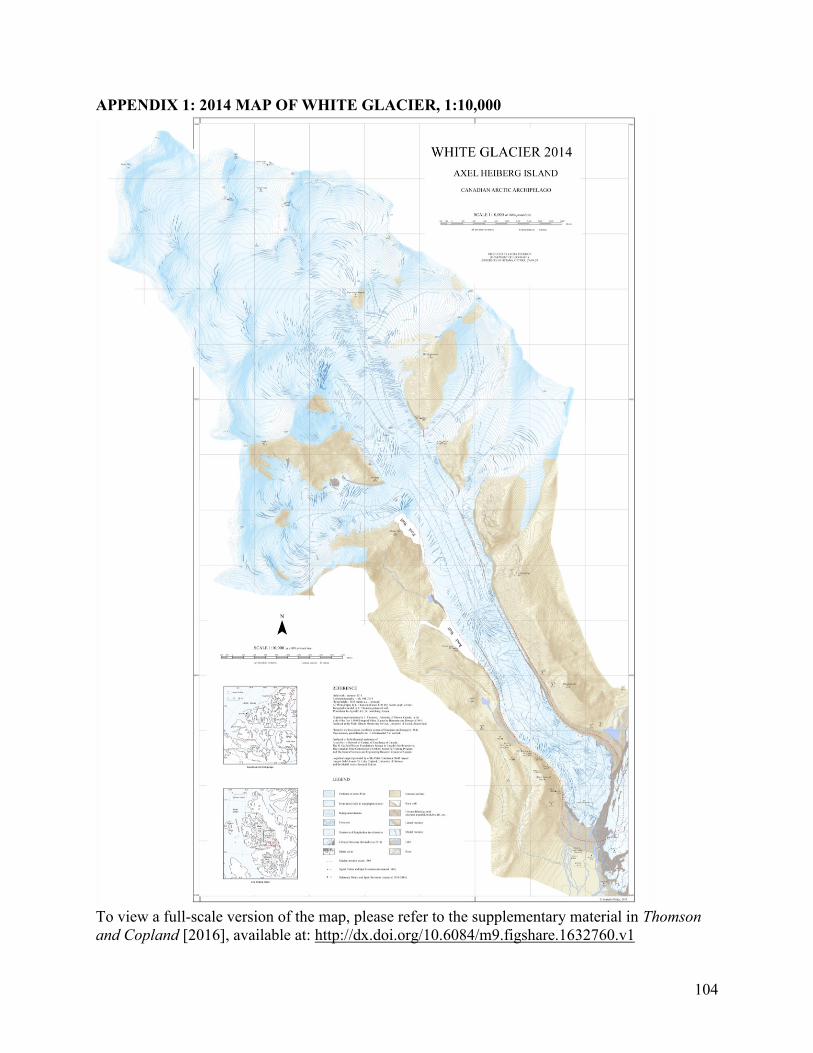
104
APPENDIX 1: 2014 MAP OF WHITE GLACIER, 1:10,000
To view a full-scale version of the map, please refer to the supplementary material in Thomson
and Copland [2016], available at: http://dx.doi.org/10.6084/m9.figshare.1632760.v1

105
APPENDIX 2: MASS BALANCE MEASUREMENT AND CALCULATION
Annual estimates of glacier mass balance at White Glacier were initiated in 1959, with the
first full year of observations being completed in 1960. These studies have continued on a yearly
basis to the present day (2016), with the exception of a three year gap from 1980-1982. Stake
measurements are made during the spring field season in April/May. In the last decade (2005-
2015) the number mass balance stake measurements located primarily along the glacier centreline
(Figure 3.1, Chapter 3) has been close to 40, which amounts to a sampling density of approximately
one stake per square kilometer. However, between 1960 and 1980, the number of stakes often
exceeded 60, with a record number of 115 mass balance measurements in 1962. These
observations occurred at the height of the Jacobsen-McGill Arctic Research Expedition and
maintaining this number of stakes was possible only because members of the research expedition
camped on the glacier at a number of sites (e.g. at Moraine Camp and Lower Ice Station) through
the months of April to August in 1960-1962 (Miles Ecclestone and Peter Adams, personal
communication). These measurements supported early studies of spatial variability in the
accumulation and ablation zones [Andrews, 1964; Havens et al., 1965, Adams, 1966] and glacier
facies [Müller, 1962].
Stake measurement methods
Snow accumulation measurements use the stratigraphic method in which the internal layers
of snow pits are characterized by thickness, hardness, crystal size and structure, and density that
is acquired by measuring with a spring-scale the mass of a cylinder (having a known volume and
weight) containing a snow sample from a given stratigraphic layer in a snow pit. At times it is
necessary to estimate the density of a layer when it is particularly thin and/or hard (e.g. for an ice
lens in the snowpack). The accumulation in a layer (in mm w.e.) is calculated from the product of
the layer thickness and density. The total accumulation, noted as positive balance, for a specific
stake is then calculated by summing the accumulation of all layers. It is possible to recognize the
previous summer surface (which should define the bottom of the snow pit) by a layer of well-
developed hoar frost and cup-shaped crystals [Müller, 1961] overlaying firn or glacier ice. The
elevation at which the base of the snow pit transitions from firn to glacier ice is indicative of
transition from accumulation to ablation conditions with decreasing elevation, and therefore is
useful in identifying the equilibrium zone of the previous year. Ablation measurements are
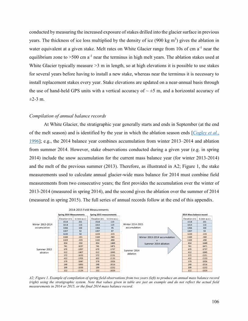
106
conducted by measuring the increased exposure of stakes drilled into the glacier surface in previous
years. The thickness of ice loss multiplied by the density of ice (900 kg m3) gives the ablation in
water equivalent at a given stake. Melt rates on White Glacier range from 10s of cm a-1 near the
equilibrium zone to >500 cm a-1 near the terminus in high melt years. The ablation stakes used at
White Glacier typically measure >3 m in length, so at high elevations it is possible to use stakes
for several years before having to install a new stake, whereas near the terminus it is necessary to
install replacement stakes every year. Stake elevations are updated on a near-annual basis through
the use of hand-held GPS units with a vertical accuracy of ~ ±5 m, and a horizontal accuracy of
±2-3 m.
Compilation of annual balance records
At White Glacier, the stratigraphic year generally starts and ends in September (at the end
of the melt season) and is identified by the year in which the ablation season ends [Cogley et al.,
1996]; e.g., the 2014 balance year combines accumulation from winter 2013–2014 and ablation
from summer 2014. However, stake observations conducted during a given year (e.g. in spring
2014) include the snow accumulation for the current mass balance year (for winter 2013-2014)
and the melt of the previous summer (2013). Therefore, as illustrated in A2; Figure 1, the stake
measurements used to calculate annual glacier-wide mass balance for 2014 must combine field
measurements from two consecutive years; the first provides the accumulation over the winter of
2013-2014 (measured in spring 2014), and the second gives the ablation over the summer of 2014
(measured in spring 2015). The full series of annual records follow at the end of this appendix.
A2; Figure 1. Example of compilation of spring field observations from two years (left) to produce an annual mass balance record
(right) using the stratigraphic system. Note that values given in table are just an example and do not reflect the actual field
measurements in 2014 or 2015, or the final 2014 mass balance record.
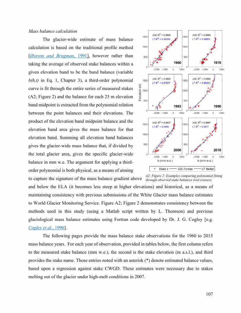
107
Mass balance calculation
The glacier-wide estimate of mass balance
calculation is based on the traditional profile method
[Østrem and Brugman, 1991], however rather than
taking the average of observed stake balances within a
given elevation band to be the band balance (variable
b(h,t) in Eq. 1, Chapter 3), a third-order polynomial
curve is fit through the entire series of measured stakes
(A2; Figure 2) and the balance for each 25 m elevation
band midpoint is extracted from the polynomial relation
between the point balances and their elevations. The
product of the elevation band midpoint balance and the
elevation band area gives the mass balance for that
elevation band. Summing all elevation band balances
gives the glacier-wide mass balance that, if divided by
the total glacier area, gives the specific glacier-wide
balance in mm w.e. The argument for applying a third-
order polynomial is both physical, as a means of aiming
to capture the signature of the mass balance gradient above
and below the ELA (it becomes less steep at higher elevations) and historical, as a means of
maintaining consistency with previous submissions of the White Glacier mass balance estimates
to World Glacier Monitoring Service. Figure A2; Figure 2 demonstrates consistency between the
methods used in this study (using a Matlab script written by L. Thomson) and previous
glaciological mass balance estimates using Fortran code developed by Dr. J. G. Cogley [e.g.
Cogley et al., 1996].
The following pages provide the mass balance stake observations for the 1960 to 2015
mass balance years. For each year of observation, provided in tables below, the first column refers
to the measured stake balance (mm w.e.), the second is the stake elevation (m a.s.l.), and third
provides the stake name. Those entries noted with an asterisk (*) denote estimated balance values,
based upon a regression against stake CWGD. These estimates were necessary due to stakes
melting out of the glacier under high-melt conditions in 2007.
A2; Figure 2: Examples comparing polynomial fitting
through observed stake balances (red crosses).
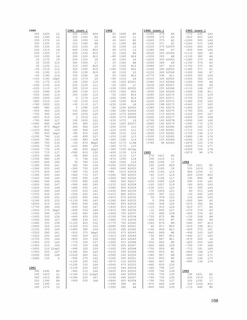
108
1960
350 1425 L1
340 1390 L2
250 1370 L3
300 1350 L4
300 1330 L5
250 1310 L6
200 1300 L7
120 1290 L8
20 1270 L9
20 1250 L10
20 1230 L11
-50 1210 L12
-50 1190 L13
-50 1180 L14
-150 1185 Cxpf
-50 1170 L15
-290 1150 L16
-220 1110 L17
-220 1090 L18
-250 1060 L19
-450 1030 L20
-680 1010 L21
-780 1000 L22
-680 980 L23
-550 960 L24
-750 940 L25
-850 910 L26
-750 890 L27
-1080 880 L28
-820 870 Mxpf
-1320 860 L29
-780 830 Dxpf
-1290 790 L32
-1620 780 L33
-1680 765 L34
-1450 750 L35
-1620 735 L36
-1300 715 L37
-1250 695 L38
-1550 680 L39
-1450 665 L40
-1380 650 L41
-1360 635 L42
-1370 620 L43
-1360 605 L44
-1420 590 L45
-1680 560 L46
-1650 540 L47
-1600 520 L48
-1420 460 L49
-1550 450 L50
-1650 430 L51
-2180 420 L52
-2020 410 L53
-1750 380 L54
-1820 375 Axpf
-1550 360 L55
-1450 355 L56
-1600 350 L57
-1680 335 L58
-1800 320 L59
-2150 305 L60
-2320 280 L61
-1920 250 L63
-2750 235 L64
-1950 220 L65
-1950 210 L66
-1850 210 LIxpf
-1950 205 L67
-2450 200 L68
-2680 100 h
1961
390 1490 B0
190 1425 L1
360 1415 B2
320 1390 B4
160 1390 L2
160 1370 L3
1961 (cont.)
350 1360 B24
300 1360 B6
160 1350 L4
310 1340 B8
220 1330 L5
440 1330 B22
200 1330 B10
300 1320 B12
250 1310 L6
360 1300 L7
310 1300 B20
320 1295 B16
300 1290 B18
330 1290 L8
220 1270 L9
190 1250 L10
220 1230 L11
300 1210 L12
280 1190 L13
300 1180 L14
0 1170 L15
-30 1150 L16
-30 1110 L17
0 1090 L18
330 1060 L19
500 1030 L20
0 1010 L21
190 1000 L22
390 980 L23
360 960 L24
140 940 L25
-80 910 L26
-60 890 L27
-140 880 L28
-60 870 Mxpf
-410 860 L29
-80 830 Dxpf
-580 810 L30
-60 800 L31
0 790 L32
30 780 L33
360 765 L34
-360 750 L35
-380 735 L36
-440 715 L37
-600 695 L38
-550 680 L39
-580 665 L40
-440 650 L41
-520 635 L42
-500 620 L43
-1020 605 L44
-1130 590 L45
-800 560 L46
-630 540 L47
-600 520 L48
-550 460 L49
-660 450 L50
-880 430 L51
-1100 420 L52
-1320 410 L53
-1080 380 L54
-910 375 Axpf
-630 350 L55
-850 355 L56
-770 350 L57
-720 335 L58
-990 320 L59
-1380 305 L60
-1020 280 L61
-990 270 L62
-1160 250 L63
-1290 235 L64
-1100 220 L65
-940 210 L66
-1160 210 LIxpf
-1380 205 L67
-990 200 L68
1962
20 1490 B0
40 1425 L1
40 1421 B2
10 1390 B4
30 1390 L2
40 1370 L3
20 1360 B6
-80 1360 B24
40 1350 L4
10 1340 B8
20 1330 B10
-180 1330 B22
40 1330 L5
20 1320 B12
-40 1310 L6
-60 1305 62001
-50 1300 L7
-100 1300 62002
-230 1300 B20
-50 1300 B14
-260 1295 B16
-140 1290 B18
-250 1290 L8
-60 1290 62003
-180 1280 62004
-240 1275 62005
-260 1275 62006
-230 1270 L9
-240 1265 62007
-200 1250 L10
-220 1230 L11
-280 1210 L12
-250 1190 L13
-340 1180 L14
-620 1175 L14A
-340 1170 L15
-380 1160 62Cxp
-690 1150 L16
-610 1110 L17
-670 1090 L18
-660 1060 L19
-1000 1055 62022
-900 1040 62023
-780 1015 62024
-1060 990 62025
-1060 960 62026
-960 945 62027
-1210 920 62028
-1080 900 62029
-1430 890 62030
-1410 885 62031
-1810 875 62032
-1280 860 62033
-1940 855 62034
-1820 810 62035
-1810 780 62036
-1660 755 62037
-2190 740 62038
-1960 710 62039
-1770 700 62040
-2080 695 62041
-2120 685 62042
-2120 675 62043
-1910 645 62044
-2360 620 62045
-1900 615 62046
-1700 605 62047
-1920 595 62048
-2220 590 62049
-2580 560 62050
-2300 545 62051
-2070 510 62052
-2040 475 62053
-2120 460 62054
-2620 455 62055
-2240 445 62056
-3190 445 62057
-2860 405 62058
-1990 386 A5
-1990 382 A4
1962 (cont.)
-1940 379 A6
-2090 376 A3
-2460 375 A2
-2330 371 A1
-2320 370 62059
-2380 366 A7
-2020 365 62060
-1930 359 A8
-2020 350 62062
-2300 349 A9
-2480 347 A10
-2240 345 62063
-2220 340 62064
-2770 338 A11
-2310 320 62065
-2580 310 62066
-2430 280 62067
-2050 255 62068
-3000 240 62069
-2080 220 62070
-2000 205 62071
-2220 200 62072
-2260 198 62073
-2380 195 62074
-2320 180 62075
-2390 175 62076
-2400 165 62077
-2790 165 62078
-2860 160 62079
-2720 145 62080
-2780 140 62081
-3000 125 62082
-3500 110 62083
-3900 105 62084
-3780 98 62085
1963
270 1421 B2
290 1419 L1
260 1294 L7
290 1269 B20
60 1185 CP
150 1165 L15
-40 1147 L16
10 1108 L17
-250 1085 L18
-160 1057 L19
-230 1031 L20
-70 1009 L21
-300 997 L22
50 978 L23
0 958 L24
-100 936 L25
-110 910 L26
-10 890 L27
-70 880 L28
-720 875 M8
-400 875 M7
-240 874 M9
40 871 M10
-100 869 M13
-440 869 M6
-50 867 M12
30 867 M11
-550 862 M5
-600 860 L29
-700 859 M2
-650 859 M1
-380 857 M4
-610 855 M3
-460 847 MD
-460 830 L30
-360 795 L31
-500 760 L34
-190 745 L35
-740 720 L36
-790 700 L37
-970 680 L38
-800 660 L39
1963 (cont.)
-770 635 L41
-820 605 L43
-1240 585 L44
-1240 510 L48
-1020 460 L49
-930 445 L50
-1110 386 A5
-1130 382 A4
-1280 379 A6
-1190 376 A3
-1700 375 A2
-1380 371 A1
-1300 366 A7
-1450 365 L54
-1020 360 L55
-1240 359 A8
-1550 348 A9
-1110 346 L57
-1660 338 A11
-1030 315 L59
-1700 274 L61
-1360 250 L63
-1440 217 L65
-1440 207 L66
-1740 206 LD
-1330 205 L67
-2060 199 L68
-1450 183 L69
-1580 170 L70
-2090 162 L71
-1710 155 L72
-1750 146 L73
-1880 138 L74
-2260 130 L75
-2470 122 L76
-2620 114 L77
-2950 106 L78
-3070 98 L79
1964
590 1421 B2
550 1419 L1
480 1293 L7
600 1269 B20
190 844 MD
490 635 L41
180 605 L43
-40 585 L44
80 510 L48
-50 460 L49
110 445 L50
-260 384 A5
-210 382 A4
-410 377 A6
-270 376 A3
-450 376 A2
-130 358 A8
-180 349 A9
-440 347 A10
-410 338 A11
-690 272 L61
-490 243 L63
-490 217 L65
-870 206 LD
-420 205 L66
-790 197 L68
-710 181 L69
-840 168 L70
-840 162 L71
-620 144 L73
-890 136 L74
1965
190 1421 B2
200 1419 L1
250 1292 L7
220 1269 B20
-110 840 MD

109
1965 (cont.)
-280 697 L37
-300 677 L38
-300 657 L39
-270 632 L41
-150 602 L43
-670 508 L48
-610 458 L49
-930 440 L50
-790 384 A5
-1020 384 A6c
-790 381 A4
-1200 379 A3c
-940 376 A3
-1060 371 A1
-820 361 A7
-870 357 A8
-940 350 A9c
-830 349 A9
-1020 324 L57
-1110 302 L59
-1450 205 30mc
-1870 204 Cc
-1480 160 L71c
1966
360 1421 B2
330 1418 L1
310 1291 L7
300 1269 B20
10 871 M7
0 863 M6
-520 859 M1
-420 857 M2
-200 853 M5
-130 848 M4
-140 848 M3
-160 837 MD
-490 695 L37
-690 675 L38
-830 655 L39
-750 630 L41
-660 600 L43
-1020 381 A5
-1010 379 A4
-1200 378 A6c
-1290 378 A3c
-1180 376 A3
-1220 371 A1
-1250 368 L54
-1110 358 A7
-990 355 A8
-1230 350 L55
-1200 349 A9c
-1280 349 A9
-1350 332 L56
-1030 321 L57
-1300 303 L58
-1300 295 L59
-1580 276 L115
-1430 268 L114
-1370 260 L113
-1510 244 L112
-1710 228 L108
-1160 226 L107
-1370 225 L106
-1560 214 L105
-1490 204 L100
-1480 204 30mc
-1540 203 Cc
-1720 202 L109
-1550 188 L101
-1780 179 L110
-1440 164 L102
-1520 160 L71c
-1660 154 L111
-1800 148 L103
1967
320 1421 B2
360 1418 L1
410 1290 L7
330 1270 B20
250 868 M13
-90 868 M7
300 865 M12
40 865 M9
240 860 M10
50 860 M6
20 856 M2
-20 849 M5
-20 845 M4
90 845 M3
40 835 MD
-80 815 L30
-130 790 L31
-490 505 L48
-470 455 L49
-760 432 L122
-900 378 A3c
-830 375 A6c
-910 350 L118
-1030 276 L115
-1250 268 L114
-970 225 L106
-1240 204 30mc
-1540 202 Cc
-1220 158 L71c
1968
100 1421 B2
160 1417 L1
110 1289 L7
150 1270 B20
-270 1037 L19
-410 1012 L20
-560 989 L21
-420 975 L22
-350 953 L23
-410 931 L24
-520 910 L25
-660 894 L26
-640 875 L28
-950 856 M6
-1410 856 M2
-970 845 M5
-1390 843 M3
-1120 840 M4
-1000 795 L30
-1590 630 W6
-1540 630 W5
-1650 627 W4
-1500 623 W3
-1020 614 W2
-1510 607 W1
-2200 390 a5
-1880 387 a6
-1860 386 a4
-2210 380 a3
-1810 377 A3c
-2090 376 a2
-1790 373 a7
-1680 371 A6c
-1910 362 a8
-1810 348 A9c
-2310 276 L115
-2410 269 K6
-1980 264 L114
-2340 255 L113
-2380 239 K5
-2000 238 L112
-2200 225 L107
-1930 223 L106
-2300 213 K1
-1990 211 L105
-2480 203 L100
-1840 203 30mc
-2360 182 K2
1968 (cont.)
-2110 158 L71
-2660 148 L103
1969
420 1420 B2
390 1417 L1
410 1288 L7
400 1271 B20
370 1130 L16
300 1085 L17
270 968 L22
200 947 L23
150 925 L24
130 903 L25
130 888 L26
-220 881 L27
-310 880 m8
-300 878 m7
-100 874 m6
-50 867 m5
-160 864 m4
-250 863 m2
-240 862 m3
-540 852 M6
-240 842 M5
-90 841 M3
-320 795 L30
-720 630 W6
-800 630 W5
-800 628 L40
-640 627 W4
-530 622 W3
-890 615 W2
-820 614 L41
-880 601 L42
-700 500 L48
-1070 409 L122
-1750 396 L121
-1240 390 a5
-1400 387 a6
-1290 382 a4
-1190 379 a3
-1540 376 a2
-1370 376 A3c
-970 376 A4
-1070 376 A3
-1340 374 a1
-1490 374 A2
-1460 373 A1
-1360 373 A5
-1400 372 a7
-1320 368 A6c
-1380 363 A6
-1290 362 a8
-1340 354 A8
-1210 353 A7
-1060 350 A9
-1570 349 a10
-1390 348 a9
-1440 348 A9c
-1610 285 L116
-1640 276 L115
-1400 260 L114
-1620 259 K6
-1570 251 L113
-1570 238 K5
-1540 227 C3
-1710 222 L107
-1440 220 L106
-1390 216 C2
-1530 212 K1
-1470 209 L105
-1580 203 L100
-1830 201 K2
-1730 193 KX
-1770 186 KY
-1680 182 K3
-1750 171 C1
-1730 160 K4
-1830 145 L103
1970
280 1420 B2
260 1418 L1
300 1363 L4
210 1288 L7
200 1271 B20
170 1213 L11
190 1128 L16
170 1082 L17
150 1050 L18
60 1030 L19
20 1007 L20
190 983 L21
200 965 L22
110 946 L23
-40 923 L24
-40 902 L25
-210 885 L26
-180 880 m8
-10 880 m7
-230 877 L27
-180 873 m6
-220 865 m5
-330 863 m2
-190 862 m4
-330 860 m3
-250 710 L35
-620 625 W6
-690 624 W5
-690 624 W4
-670 621 W3
-570 615 W2
-1040 407 L122
-1090 395 L121
-850 389 a5
-1100 385 a6
-1020 378 a4
-970 376 A4
-1190 376 A3
-1280 375 a2
-1210 373 A1
-800 372 A5
-1060 370 a7
-930 351 A9
-740 351 A8
-1270 348 a10
-770 348 a9
-1470 285 L116
-1210 277 L115
-1260 260 L114
-1210 260 K6
-1170 251 L113
-1300 238 K5
-1080 233 L112
-1370 227 C3
-1110 224 L107
-1130 220 L106
-1110 216 C2
-1210 212 K1
-1240 209 L105
-1390 205 K2
-1570 204 L100
-1220 191 KX
-1270 186 KY
-1320 183 K3
-1350 178 P
-1230 170 C1
-1270 160 K4
-1350 144 L103
1971
340 1420 B2
270 1418 L1
210 1287 L7
230 1271 B20
180 1126 L16
150 1078 L17
120 1046 L18
0 1026 L19
-60 1003 L20
1971 (cont.)
-250 979 L21
-220 961 L22
-430 941 L23
-390 918 L24
-480 899 L25
-540 883 L26
-850 878 m8
-710 877 m7
-560 870 m6
-850 862 m5
-850 859 m4
-1180 857 m3
-1140 736 L34
-1030 709 L35
-1130 620 W
-1560 471 L48
-1580 461 L126
-1490 456 L125
-1500 443 L124
-1550 428 L123
-1480 405 L122
-1690 387 a5
-1650 382 a6
-1480 373 a1
-1630 370 a5
-1610 359 a8
-1470 359 a6
-1440 353 a7
-1540 350 a9
-1180 350 a8
-1790 348 a10
-1750 348 a9
-1740 276 L115
-1410 259 L114
-1750 250 K5
-1640 220 L106
-1680 209 L105
-1990 205 K2
-2190 183 K3
-2140 170 C1
-1910 160 K4
-2310 144 L103
1972
300 1420 B2
320 1419 L1
270 1360 L4
210 1285 L7
210 1270 B20
260 1210 L11
250 1123 L16
200 1074 L17
200 1042 L18
210 1001 L20
140 974 L21
230 956 L22
340 936 L23
320 913 L24
160 884 L25
120 880 L26
40 876 m8
-30 874 m7
150 872 L27
110 867 m6
110 859 m5
180 859 m2
150 856 m4
140 855 m3
100 849 mD
80 733 L34
190 708 L35
120 691 L36
-30 672 L37
-70 651 L38
90 637 L39
-30 624 L40
140 621 W6
120 620 W5
100 620 W4

110
1972 (cont.)
120 619 W3
40 616 W2
-320 477 L47
-110 470 L48
-550 459 L126
-400 454 L125
-710 441 L124
-820 426 L123
-580 403 L122
-720 392 L121
-500 385 a5
-850 379 a6
-490 378 a3
-710 377 a2
-800 375 A2
-760 373 A3
-920 373 A1
-560 373 a4
-290 373 a1
-420 372 A4
-490 368 A5
-570 366 a7
-730 360 a8
-510 357 A6
-430 352 A7
-820 349 A9
-410 349 A8
-1140 348 a10
-330 348 a9
-920 311 L118
-970 283 L116
-840 275 L115
-920 260 K6
-970 258 L114
-1030 250 L113
-890 238 K5
-1000 232 L112
-940 227 C3
-1110 224 L107
-1200 220 L106
-1210 216 C2
-1030 212 K1
-1210 209 L105
-1460 205 K2
-1500 204 L100
-1220 201 L111
-1290 191 KX
-1170 190 KZ
-1010 186 KY
-1300 183 K3
-1250 170 C1
-1340 160 K4
-1350 152 L104
-1580 144 L103
-1530 129 L101
-1930 112 L102
1973
350 1420 B2
450 1418 L1
300 1284 L7
410 1270 B20
330 1210 L11
350 1120 L16
370 1070 L17
340 1001 L20
330 891 L25
310 881 L26
360 874 m8
150 871 m7
120 869 L27
150 863 m6
250 856 m5
40 856 m2
90 852 m3
120 852 m4
-80 845 mD
180 729 L34
110 706 L35
1973 (cont.)
-130 690 L36
-330 668 L37
-290 648 L38
-240 634 L39
-210 619 W6
-200 619 W3
-180 618 W5
-270 618 W4
-330 616 W2
-580 474 L47
-400 467 L48
-860 414 L123
-930 399 L122
-1070 395 Drill
-710 380 a5
-540 376 a3
-850 374 L121
-710 373 a1
-980 371 a6
-1170 370 A3
-830 369 a4
-790 357 a8
-720 350 A7
-690 349 A9
-750 347 a9
-630 346 A8
-790 304 L118
-1100 184 KY
1974
210 1419 B2
190 1417 L1
200 1283 L7
200 1270 B20
170 1118 L16
150 1068 L17
-180 992 L20
10 947 L22
-90 927 L23
-70 905 L24
-190 888 L25
-280 879 L26
-310 872 m8
-270 869 m7
-250 866 L27
-230 862 m6
-510 854 m2
-150 853 m5
-220 850 m3
-280 848 m4
-300 841 mD
-400 726 L34
-290 703 L35
-400 685 L36
-470 665 L37
-570 645 L38
-540 631 L39
-650 618 W3
-730 616 W6
-630 616 W5
-730 615 W2
-840 350 A7
-920 345 A8
-1080 304 L116
-1120 282 L115
-1140 271 L114
-1170 255 K5
-1340 253 L113
-1210 240 L112
-1180 220 L111
-1220 220 K1
-1400 208 L107
-1570 205 C2
-1140 205 L106
-1300 202 L100
-1380 184 KY
-1360 171 C1
-1660 160 L103
1975
640 1419 B2
610 1417 L1
490 1282 L7
530 1279 B20
410 1116 L16
470 1063 L17
190 988 L20
360 962 L21
250 899 L24
120 877 L26
230 872 m12
0 866 m7
100 859 m6
10 850 m5
-60 847 m3
100 845 m4
-10 838 mD
-50 722 L34
-190 701 L35
-230 682 L36
-290 662 L37
-310 642 L38
-240 629 L39
-330 617 W3
-360 615 W4
-330 615 W2
-240 614 W6
-220 614 W5
-940 466 L48
-750 454 L126
-940 432 L124
-1030 397 L122
-1090 378 a5
-1040 378 a4
-910 375 a3
-1160 372 L121
-1350 368 A3
-940 368 a6
-1180 362 A5
-740 358 a7
-1110 355 a8
-970 352 A6
-1000 349 A7
-940 347 a9
-780 345 A8
-1120 328 L118
-970 312 L117
-1150 301 L116
-1300 280 L115
-1430 269 L114
-1170 253 K5
-1250 250 L113
-1330 235 L112
-1380 218 K1
-1230 216 L111
-1480 204 L107
-1250 202 L106
-1500 198 L100
-1210 189 KZ
-1490 183 KY
-1570 168 C1
-1570 159 L104
-1670 156 L103
1976
330 1419 B2
290 1416 L1
340 1281 L7
340 1278 B20
180 897 L24
170 882 L25
90 875 L26
-150 865 m8
0 860 m7
10 855 m6
0 845 m5
-220 843 m4
-80 832 mD
-30 698 L35
1976 (cont.)
-120 676 L36
-200 659 L37
-120 640 L38
-270 628 L39
-130 616 W3
-230 614 W4
10 614 W2
-170 613 W6
-380 613 W5
-1020 465 L48
-820 448 L126
-950 428 L124
-820 376 a4
-610 375 a5
-860 374 a3
-1040 370 a1
-800 370 L121
-1060 368 A1
-1150 365 a6
-720 365 A3
-930 360 A5
-730 356 a7
-560 353 a8
-480 350 A8
-720 350 A6
-740 346 a9
-570 345 A7
-1130 325 L118
-1080 298 L116
-930 280 L115
-1150 268 L114
-1040 250 K5
-1130 245 L113
-1030 238 K3
-1020 230 L112
-1110 220 L109
-1150 216 K1
-1140 211 L111
-1090 210 L108
-930 201 L107
-1020 198 L106
-1210 195 L110
-1190 195 L100
-1050 180 L105
-1210 175 KY
-1250 165 C1
-1140 160 KX
-1300 155 L104
-1130 150 L102
-1500 130 L103
-1570 130 L101
1977
120 1418 B2
150 1415 L1
130 1280 L7
100 1277 B20
90 1112 L16
-150 955 L21
-260 935 L22
-450 915 L23
-490 893 L24
-570 879 L25
-1300 850 m6
-1360 849 m2
-970 842 m3
-1080 841 m5
-1010 840 m4
-1030 828 mD
-1070 760 L32
-1230 726 L33
-1530 705 L34
-1430 694 L35
-1720 672 L36
-1800 656 L37
-1740 626 L39
-1730 613 W9
-1840 613 W3
-1700 612 W2
1977 (cont.)
-1770 611 W8
-1860 611 W4
-1700 609 W7
-1800 609 W5
-1700 608 W11
-1790 608 W6
-2460 501 L44
-2200 481 L45
-2060 474 L46
-2200 463 L48
-2270 444 L126
-2240 423 L124
-2240 393 L122
-2020 373 a4
-2340 373 a3
-2540 369 a1
-2090 368 L121
-2940 368 A1
-2380 365 A4
-2720 365 A3
-2050 362 a6
-2390 357 A5
-1860 353 a7
-1970 350 a8
-2140 349 A8
-2170 347 A6
-2300 345 a9
-2200 342 A7
-2410 322 L118
-2310 295 L116
-2370 278 L115
-2290 267 L114
-2390 248 K5
-2430 241 L113
-2290 227 L112
-2490 219 L109
-2220 215 K1
-2370 210 L111
-2560 208 L108
-2480 201 L107
-2260 197 L106
-2730 194 L100
-2360 192 L110
-2530 172 KY
-2450 163 C1
-2420 157 KX
-2330 153 L104
-2470 147 L102
-2790 127 L103
-2730 127 L101
1978
240 1415 L1
260 1280 L7
200 1277 B20
250 1109 L16
-90 952 L21
-170 932 L22
-130 912 L23
-70 890 L24
-400 876 L25
-890 839 m3
-630 838 m5
-700 837 m4
-1060 653 L37
-1110 636 L38
-1030 624 L39
-1010 612 W2
-1140 612 W3
-1100 610 W11
-1130 608 W4
-1110 608 W8
-1130 605 W5
-1130 605 W6
-1820 160 C1

111
1979
200 1418 B2
180 1415 L1
200 1279 L7
200 1276 B20
180 1165 L12
200 1106 L16
80 975 L20
30 950 L21
-30 930 L22
-80 910 L23
-250 874 L25
-200 835 m5
-630 835 m4
-660 760 L32
-580 725 L33
-670 695 L34
-670 652 L37
-890 635 L38
-850 622 L39
-820 611 W11
-1040 610 W10
-690 610 W2
-1000 608 W3
-850 602 W4
-1020 601 W9
-770 597 W5
-860 596 W8
-910 594 W7
-690 594 W6
-1080 580 L41
-1090 466 L47
-1300 425 L124
-1440 385 L122
-1030 372 a4
-1240 370 a3
-1490 370 a1
-1030 369 a5
-1050 365 L121
-1430 360 A3
-950 360 a6
-1230 360 L120
-1230 355 A9
-940 355 a8
-1030 353 a9
-1000 352 A8
-1210 348 A5
-1000 340 L119
-1300 320 L118
-1250 299 L116
-1300 280 L115
-1750 270 L114
-1350 265 78-1
-1600 260 78-2
-1320 238 K3
-1230 220 78-4
-1490 210 78-5
-1370 210 L106
-1450 195 78-9
-1410 190 78-8
-1320 175 KZ
-1550 160 KX
-1360 155 L102
-1650 130 78-12
1983
230 1460 Extra
290 1340 L1
190 1285 ?
240 1235 Blue
230 1205 M2
240 1165 L16
180 1110 L17
90 1045 L18
220 1020 L19
170 975 L20
160 955 L21
160 935 L22
80 925 L23
-1140 620 CWGH
1983 (cont.)
-1660 380 CWGF
-1280 380 CWGF1
-1660 260 CWGE
-2440 230 OWPA1
-1610 220 CWGD
-1620 210 WG4
-2000 180 CWGB
-2020 165 CWGA
-1520 155 WG3
-1620 140 OWPA2
-1890 115 WG1
-2100 110 WG2
1984
260 1590 CJA1
530 1460 Extra
230 1340 L1
200 1285 ?
230 1235 Blue
190 1205 M2
230 1165 L16
40 1110 L17
40 1045 L18
190 1020 L19
80 975 L20
90 955 L21
40 935 L22
50 925 L23
-1140 620 CWGH
-1050 380 CWGF
-1130 380 CWGF1
-1570 260 CWGE
-1420 230 OWPA1
-1610 220 CWGD
-1040 210 WG4
-1660 180 CWGB
-1750 165 CWGA
-2100 155 WG3
-2700 140 OWPA2
-2480 115 WG1
-2760 110 WG2
1985
260 1590 CJA1
370 1510 DCP1
210 1460 Extra
430 1340 L1
210 1285 ?
200 1235 Blue
150 1205 M2
210 1165 L16
30 1110 L17
20 1045 L18
140 1020 L19
50 975 L20
70 955 L21
70 935 L22
50 925 L23
-1050 380 CWGF
-1130 380 CWGF1
-1570 260 CWGE
-1430 230 OWPA1
-1620 220 WG5
-1610 220 CWGD
-1040 210 WG4
-1660 180 CWGB
-1750 165 CWGA
-1990 155 WG3
-2460 140 OWPA2
-1980 115 WG1
-2760 110 WG2
1986
320 1590 CJA1
350 1510 DCP1
260 1460 Extra
230 1340 L1
1986 (cont.)
190 1285 ?
240 1235 Blue
240 1205 M2
170 1165 L16
140 1110 L17
70 1045 L18
140 1020 L19
50 975 L20
90 955 L21
80 935 L22
100 925 L23
-1360 735 CWGEx
-2080 625 CWGG
-1860 620 CWGK
-2190 620 CWGH
-1740 615 CWGL
-1890 380 CWGF
-2030 380 CWGF1
-3140 260 CWGE
-2660 230 OWPA1
-2270 220 CWGD
-2920 220 WG5
-1870 210 WG4
-2990 180 CWGB
-3120 165 CWGA
-3390 155 WG3
-3480 140 OWPA2
-3400 115 WG1
-3070 110 WG2
1987
60 1590 CJA1
90 1510 DCP1
70 1460 Extra
-240 1340 L1
-330 1285 ?
-290 1235 Blue
-370 1205 M2
-540 1165 L16
360 1110 L17
-500 1045 L18
-490 975 L20
-380 955 L21
170 935 L22
-560 925 L23
-1360 735 CWGEx
-1740 620 CWGK
-1740 620 CWGH
-2090 615 CWGL
-1800 380 CWGF
-2260 380 CWGF1
-4240 260 CWGE
-3390 230 OWPA1
-3430 220 WG5
-3610 220 CWGD
-3390 210 WG4
-3000 180 CWGB
-4680 165 CWGA
-3500 155 WG3
-3480 140 OWPA2
-3480 115 WG1
-3480 110 WG2
1988
330 1590 CJA1
300 1510 DCP1
210 1460 Extra
220 1340 L1
280 1285 ?
230 1235 Blue
240 1205 M2
260 1165 L16
110 1110 L17
160 1045 L18
10 975 L20
240 955 L21
240 935 L22
120 925 L23
1986 (cont.)
-60 380 CWGF
-280 380 CWGF1
-820 230 OWPA1
-900 220 CWGD
-550 220 WG5
-760 210 WG4
-970 180 CWGB
-1170 165 CWGA
-1430 155 WG3
-1280 140 OWPA2
-1570 115 WG1
1989
280 1590 CJA1
250 1510 DCP1
130 1460 Extra
100 1340 L1
120 1285 ?
200 1235 Blue
130 1205 M2
190 1165 L16
-30 1110 L17
30 1045 L18
20 1020 L19
20 975 L20
70 955 L21
120 935 L22
20 925 L23
-150 625 CWGG
40 620 CWGK
40 620 CWGH
-110 615 CWGL
-60 380 CWGF
-630 260 CWGE
-840 230 OWPA1
-650 220 CWGD
-550 220 WG5
-840 210 WG4
-770 180 CWGB
-720 165 CWGA
-1380 155 WG3
-1580 140 OWPA2
-1560 115 WG1
-1940 110 WG2
1990
120 1590 CJA1
150 1510 DCP1
-20 1460 Extra
-40 1340 L1
-50 1285 ?
-70 1235 Blue
-80 1205 M2
-90 1165 L16
-590 1110 L17
-370 1045 L18
-230 1020 L19
-630 975 L20
-700 955 L21
-450 935 L22
-770 925 L23
-930 735 CWGEx
-1130 625 CWGG
-1280 620 CWGK
-1740 380 CWGF1
-1760 220 CWGD
-1720 220 WG5
-1800 210 WG4
-2160 180 CWGB
-2060 165 CWGA
-2740 155 WG3
-2790 115 WG1
-2740 110 WG2
1991
320 1590 CJA1
250 1510 DCP1
1991 (cont.)
160 1460 Extra
150 1340 L1
80 1285 ?
80 1235 Blue
40 1205 M2
80 1165 L16
0 1110 L17
0 1045 L18
40 1020 L19
-170 975 L20
-170 955 L21
-140 935 L22
-370 925 L23
-620 735 CWGEx
-950 625 CWGG
-780 620 CWGK
-890 380 CWGF
-1470 220 CWGD
-1500 220 WG5
-2370 210 WG4
-1870 180 CWGB
-1650 165 CWGA
-2130 155 WG3
-3160 115 WG1
-2660 110 WG2
1992
140 1590 CJA1
150 1510 DCP1
90 1460 Extra
50 1340 L1
-100 1285 ?
-120 1235 Blue
-150 1205 M2
-70 1165 L16
-300 1110 L17
-370 1045 L18
-240 955 L21
-340 935 L22
-820 735 CWGEx
-950 380 CWGF1
-810 380 CWGF
-800 220 WG5
-920 220 CWGD
-1390 210 WG4
-1610 180 CWGB
-1210 165 CWGA
-1510 155 WG3
-2380 115 WG1
-2330 110 WG2
1993
230 1590 CJA1
200 1510 DCP1
110 1460 Extra
120 1340 L1
-160 1285 ?
-190 1235 Blue
-230 1205 M2
-110 1165 L16
-450 1110 L17
-550 1045 L18
-370 955 L21
-510 935 L22
-1230 735 CWGEx
-1430 380 CWGF1
-1450 380 CWGF
-1710 220 WG5
-1390 220 CWGD
-2500 210 WG4
-2420 180 CWGB
-2630 165 CWGA
-2470 155 WG3
-2370 115 WG1
-3510 110 WG2

112
1994
330 1590 CJA1
240 1510 DCP1
120 1460 Extra
100 1340 L1
120 1285 ?
80 1235 Blue
-70 1165 L16
-140 1110 L17
-450 1045 L18
-260 955 L21
-560 770 WG8
-920 745 WG7
-1630 380 CWGF1
-1320 380 CWGF
-1210 375 WG6
-2260 220 CWGD
-1660 220 WG5
-670 210 WG4
-1890 180 CWGB
-3680 165 CWGA
-2130 155 WG3
-3990 155 WG0
-3100 115 WG1
-2400 110 WG2
1995
330 1590 CJA1
350 1510 DCP1
260 1460 Extra
180 1340 L1
70 1285 ?
-180 1235 Blue
-50 1205 M2
-100 1165 L16
-330 1110 L17
-50 1045 L18
-300 1020 L19
-470 1020 L19A
-450 955 L21
-450 935 L22
-680 830 WG9
-860 770 WG8
-1080 735 CWGEx
-1320 660 WG7
-2460 380 CWGF1
-2160 380 CWGF
-2230 220 WG5
-2200 220 CWGD
-2840 210 WG4
-2470 180 CWGB
-2390 165 CWGA
-2760 155 WG3
-3540 115 WG1
-2760 110 WG2
-2210 110 WG0
1996
224 1485 CJA1
200 1463 LP2
267 1421 DCP1
82 1348 Extra
153 1258 L1
163 1197 ?
162 1165 Blue
30 1070 L16
63 1018 L17
108 959 L18
36 934 L19
144 920 L19A
57 877 L21
-90 869 L22
27 793 WG9
18 698 WG8
-36 658 CWGEx
-99 614 WG7
-306 462 LP8
-297 421 WG6
-333 373 LP9
1996 (cont.)
-891 310 CWGF1
-504 310 CWGF
-558 228 WG5
-580 211 CWGD
-652 193 WG4
-684 191 LP10
-1020 159 WG3
-1440 152 WG0
-756 142 CWGA
-1570 127 WG2
-1035 122 WG1
1997
472 1485 CJA1
374 1473 WPA1
329 1463 LP2
334 1437 WPA2
399 1421 DCP1
349 1381 LP4
256 1355 WPA3
328 1348 Extra
296 1325 JGC2
289 1292 WPA4
288 1275 WPA5
177 1258 L1
287 1197 ?
285 1165 Blue
345 1135 M2A
220 1070 L16
-53 1018 L17
-198 959 L18
-189 934 L19
-198 920 L19A
-459 877 L21
-144 877 L21A
-207 869 L22
-634 793 WG9
-717 750 LP5
-682 698 WG8
-639 658 CWGEx
-942 614 WG7
-1203 570 LP6
-792 462 LP8
-1143 421 WG6
-1170 372 LP9
-1260 315 CWGF
-1008 310 CWGF1
-1413 228 WG5
-891 211 CWGD
-1867 192 WG4
-1309 191 LP10
-1557 189 CWGB
-2151 159 WG3
-2268 152 WG0
-2142 152 WG0A
-1775 142 CWGA
-2592 127 WG2
-2007 121 WG1
1998
137 1525 JGC1
227 1485 CJA1
159 1473 WPA1
177 1463 LP2
159 1437 WPA2
209 1421 DCP1
115 1381 LP4
284 1355 WPA3
232 1348 Extra
172 1325 JGC2
210 1292 WPA4
232 1275 WPA5
198 1258 L1
170 1197 ?
104 1165 Blue
162 1135 M2A
91 1070 L16
-153 1018 L17
1998 (cont.)
-99 959 L18
-243 934 L19
-180 920 L19A
-297 900 L20
-369 877 L21
-315 877 L21A
-675 869 L22
-540 793 WG9
-864 750 LP5
-891 698 WG8
-873 658 CWGEx
-846 614 WG7
-855 570 LP6
-1575 462 LP8
-2016 421 WG6
-1741 372 LP9
-2376 315 CWGF
-2484 310 CWGF1
-2304 228 WG5
-2610 211 CWGD
-2749 192 WG4
-2196 191 LP10
-2189 189 CWGB
-2601 159 WG3
-3384 152 WG0
-2070 142 CWGA
-3366 127 WG2
-2133 121 WG1
1999
212 1525 JGC1
200 1485 CJA1
193 1473 WPA1
185 1463 LP2
96 1437 WPA2
203 1421 DCP1
207 1381 LP4
153 1355 WPA3
184 1348 Extra
178 1325 JGC2
169 1292 WPA4
272 1275 WPA5
184 1258 L1
134 1197 ?
96 1165 Blue
-72 1135 M2A
-532 1070 L16
-783 1018 L17
-882 959 L18
-1125 934 L19
-1008 920 L19A
-819 900 L20
-1435 793 WG9
-1755 750 LP5
-1512 698 WG8
-1575 665 CWGS
-1692 658 CWGEx
-1786 614 WG7
-1917 570 LP6
-1872 462 LP8
-1962 421 WG6
-2043 372 LP9
-2385 315 CWGF
-2667 310 CWGF1
-2142 228 WG5
-1908 211 CWGD
-2574 192 WG4
-2304 191 LP10
-2142 189 CWGB
-2232 159 WG3
-2457 152 WG0
-2277 142 CWGA
-3132 127 WG2
-2700 121 WG1
2000
130 1518 JGC1
99 1489 CJA1
45 1455 WPA1
117 1468 LP2
66 1421 WPA2
163 1423 DCP1
94 1384 LP4
71 1355 WPA3
105 1348 Extra
50 1317 JGC2
60 1291 WPA4
91 1278 WPA5
91 1266 L1
-63 1192 ?
-180 1165 Blue
-108 1120 M2
-540 1120 M2A
-774 1063 L16
-405 1063 L16A
-252 1018 L17
-675 934 L19
-594 879 L20
-621 877 L21
-720 864 L22
-1089 793 WG9
-1332 747 LP5
-936 698 WG8
-963 690 CWGT
-1350 648 CWGS
-1071 643 CWGEx
-1449 614 WG7
-1179 614 WG7A
-1188 570 LP6
-1368 570 LP6A
-1431 449 LP8
-1242 449 LP8A
-1711 403 WG6
-1611 403 WG6A
-1431 363 LP9
-3582 330 CWGF
-1944 315 CWGF1
-1854 224 WG5
-1773 196 CWGD
-2106 192 WG4
-1876 190 LP10
-1917 152 CWGB
-1998 171 WG3
-2052 152 WG0
-2187 136 CWGA
-2304 127 WG2
-3042 121 WG1
2001
242 1518 JGC1
179 1489 CJA1
186 1455 WPA1
291 1468 LP2
125 1421 WPA2
154 1423 DCP1
214 1384 LP4
144 1355 WPA3
159 1348 Extra
76 1317 JGC2
98 1291 WPA4
183 1278 WPA5
153 1266 L1
170 1192 ?
-9 1165 Blue
103 1160 Blue2
-36 1120 M2
36 1135 M2A
-126 1063 L16
-342 1065 L16A
-153 1018 L17
-333 950 L18
-108 934 L19
-301 879 L20
-297 877 L21
-360 864 L22
2001 (cont.)
-711 793 WG9
-864 747 LP5
-648 698 WG8
-630 698 WG8A
-409 690 CWGT
-567 648 CWGS
-864 643 CWGEx
-688 614 WG7
-774 570 LP6
-877 449 LP8
-1215 403 WG6A
-1201 363 LP9
-1305 315 CWGF1
-1165 251 ST4
-1219 224 WG5A
-1089 228 WG5
-1350 196 CWGD
-1210 192 WG4
-1269 192 WG4A
-1507 190 LP10
-1505 190 LP10A
-1440 152 CWGB
-1422 171 WG3
-1489 171 WG3A
-1701 152 WG0
-1377 152 WG0A
-1485 136 CWGA
-1831 127 WG2
-1813 121 WG1
2002
194 1518 JGC1
147 1489 CJA1
302 1455 WPA1
176 1468 LP2
173 1421 WPA2
168 1423 DCP1
126 1384 LP4
308 1355 WPA3
130 1348 Extra
137 1317 JGC2
263 1291 WPA4
175 1278 WPA5
243 1266 L1
-90 1192 ?
0 1165 Blue
-36 1160 Blue2
296 1135 M2A
-9 1065 L16A
468 1018 L17
468 950 L18
342 934 L19
270 879 L20
72 877 L21
0 864 L22
-261 793 WG9
-76 747 LP5
-945 698 WG8
-513 698 WG8A
-207 690 CWGT
-301 643 CWGEx
-189 614 WG7
-459 614 WG7A
-432 570 LP6
-913 449 LP8
-828 403 WG6A
-954 421 WG6
-1199 363 LP9
-1210 363 LP9A
-1278 315 CWGF1
-1246 251 ST4
-1341 251 ST4A
-1350 196 CWGD
-1845 192 WG4A
-1737 190 LP10
-2097 152 CWGB
-1786 171 WG3
-1818 159 WG3A
-981 152 WG0

113
2002 (cont.)
-432 152 WG0A
-2241 136 CWGA
-1908 127 WG2
-1962 121 WG1
2003
628 1518 JGC1
402 1489 CJA1
485 1455 WPA1
372 1468 LP2
373 1421 WPA2
532 1423 DCP1
347 1384 LP4
334 1355 WPA3
462 1348 Extra
281 1317 JGC2
388 1291 WPA4
413 1278 WPA5
324 1266 L1
540 1192 ?
571 1165 Blue
605 1160 Blue2
-216 1135 M2A
-369 1065 L16A
-360 1018 L17
-288 950 L18
-463 934 L19
-526 879 L20
-432 877 L21
-603 864 L22
-756 793 WG9
-1048 747 LP5
-913 698 WG8
-1278 690 CWGT
-1206 648 CWGS
-1134 643 CWGEx
-1287 614 WG7A
-1719 570 LP6
-1300 421 WG6
-1332 363 LP9A
-1381 251 ST4A
-1530 228 WG5
-1656 196 CWGD
-1606 192 WG4
-1683 190 LP10
-1638 190 LP10A
-2110 159 WG3A
-2191 159 WG3B
-1917 152 WG0B
-2340 136 CWGA
-1728 127 WG2
-1786 121 WG1
2004
324 1518 JGC1
283 1489 CJA1
290 1455 WPA1
225 1468 LP2
192 1421 WPA2
276 1423 DCP1
284 1384 LP4
242 1355 WPA3
258 1348 Extra
244 1317 JGC2
393 1292 WPA4
262 1278 WPA5
196 1266 L1
168 1192 ?
211 1165 Blue
153 1160 Blue2
342 1070 L16A
252 1018 L17
162 950 L18
112 934 L19D
139 900 L20
81 900 L20A
9 877 L21
-319 869 L22
2004 (cont.)
-135 793 WG9
-252 750 LP5
-306 698 WG8
-450 690 CWGT
-252 648 CWGS
-522 643 CWGEx
-639 614 WG7A
-765 570 LP6
-1066 462 LP8
-1192 421 WG6
-1102 421 WG6A
-1066 383 JP4
-1152 378 JP3
-1242 378 JP5
-1089 372 LP9
-1156 359 JP2
-648 348 JP1
-1505 310 CWGF1
-1372 251 ST4
-1323 228 WG5
-1435 228 WG5A
-1134 211 CWGD
-1705 192 WG4
-1530 190 LP10A
-1588 190 LP10B
-1764 171 WG3B
-1710 152 WG0
-1917 136 CWGA
-1764 127 WG2
-1795 127 WG2A
-1620 121 WG1
2005
353 1518 JGC1
144 1489 CJA1
269 1455 WPA1
277 1468 LP2
196 1421 WPA2
298 1423 DCP1
226 1384 LP4
380 1355 WPA3
214 1348 Extra
188 1317 JGC2
156 1291 WPA4
170 1278 WPA5
-27 1266 L1
-252 1192 ?
-333 1160 Blue2
-817 1135 M2A
-783 1065 L16A
-387 1018 L17
-747 950 L18
-1134 934 L19
-936 879 L20
-1170 877 L21
-1782 864 L22
-1755 793 WG9
-1962 698 WG8
-1836 690 CWGT
-2106 648 CWGS
-2106 643 CWGEx
-2362 421 WG6
-2997 196 CWGD
-2970 159 WG3A
-3636 136 CWGA
-3123 127 WG2
2006
422 1518 JGC1
206 1489 CJA1
186 1455 WPA1
316 1468 LP2
175 1421 WPA2
273 1423 DCP1
187 1384 LP4
266 1355 WPA3
307 1348 EXTRA
204 1317 JGC2
2006 (cont.)
200 1292 WPA4
204 1278 WPA5
266 1266 L1
246 1192 QMARK
270 1165 BLUE
175 1160 BLUE2
36 1120 M2A
135 1070 L16A
-72 1018 L17
-94 950 L18
45 934 L19D
-225 900 L20
-306 877 L21
-900 869 L22
-621 793 WG9
-540 793 WG9A
-540 750 LP5
-648 698 WG8
-486 690 CWGT
-706 648 CWGS
-594 643 CWGX
-756 614 WG7A
-1008 570 LP6
-1129 462 LP8
-1107 421 WG6
-1224 372 LP9
-1287 315 ST6
-1386 251 ST4
-1435 228 WG5
-1507 192 WG4
-1575 190 LP10A
-1984 171 WG3B
-1993 152 WG0
-2529 136 CWGA
-2277 127 WG2
-2232 121 WG1
2007
248 1521 JGC1
184 1492 CJA1
110 1458 WPA1
178 1467 LP2
72 1419 WPA2
191 1418 DCP1
148 1372 LP4
80 1348 WPA3
184 1329 EXTRA
111 1302 JGC2
100 1275 WPA4
113 1260 WPA5
97 1243 L1
-555 1171 QMARK
-749 1140 BLUE
-503 1139 BLUE2
-1100 1018 L16A
-1280 949 L17
-1030 892 L18
-1745 859 L19
-1785 843 L20
-2000 838 L21
-2510 839 L22
-2500 740 WG9
-2480 703 LP5
-2380 686 WG8
-2142 679 CWGT
-2007 620 CWGS
-2038 615 CWGX
-2560 587 WG7
-2770 568 LP6
-2835 490 LP8
-3110 422 WG6
-2480 398 LP9A
*-3220 196 WG4
*-3549 195 WG5
-3663 184 CWGD
*-3253 183 LP10
*-3630 168 WG3
-4644 132 CWGA
*-3862 127 WG1
2008
114 1521 JGC1
89 1492 CJA1
79 1458 WPA1
40 1467 LP2
12 1419 WPA2
108 1418 DCP1
91 1372 LP4
64 1348 WPA3
90 1329 EXTRA
59 1302 JGC2
84 1275 WPA4
115 126 WPA5
14 1243 L1
-73 1171 QMARK
-648 1140 BLUE
-651 1139 BLUE2
-1516 1060 L16A
-1116 949 L17
-1260 949 L17A
-1773 892 L18
-1471 906 L18A
-1642 880 L19
-1588 863 L20
-1777 851 L21A
-2038 745 WG9A
-2160 684 WG8A
-1782 667 CWGT
-2079 629 CWGS
-2169 625 CWGX
-2061 598 WG7A
-2290 575 LP6A
-2250 488 LP8A
-2142 423 WG6
-2196 398 LP9A
-2475 299 ST6
-1980 237 ST4
-2835 188 WG5
-2493 189 CWGD
-1827 184 WG4
-2682 186 LP10
-3055 157 WG3
-4770 120 CWGA
-3631 112 WG1
2009
176 1521 JGC1
156 1497 CJA1
172 1466 WPA1
173 1459 LP2
162 1414 WPA2
197 1411 DCP1
188 1381 LP4
173 1339 WPA3
241 1329 EXTRA
154 1300 JGC2
188 1273 WPA4
164 1260 WPA5
165 1238 L1
107 1228 MARK
-648 1140 BLUE
-651 1139 BLUE2
-954 1020 L16A
-981 1018 L16D
-873 1016 L16E
-913 966 L17A
-1084 906 L18A
-1287 859 L19
-1305 845 L20
-1332 836 L21A
-1449 703 LP5
-1476 680 WG8A
-1359 667 CWGT
-1620 621 CWGX
-1575 598 WG7A
-2767 575 LP6A
-2092 488 LP8A
-2133 423 WG6
-2119 382 LP9A
-2241 293 ST6
2009 (cont.)
-2317 237 ST4
-2610 188 WG5
-2376 177 CWGD
-2637 190 WG4
-2542 180 LP10
-2817 154 WG3
-3348 112 WG1
2010
431 1520 JGC1
250 1486 CJA1
255 1455 WPA1
276 1479 LP2
231 1449 WPA2
283 1441 DCP1
110 1364 LP4
343 1343 WPA3
376 1329 EXTRA
261 1308 JGC2
325 1273 WPA4
252 1261 WPA5
211 1228 L1
255 1160 QMARK
-54 1126 BLUE
-90 1129 BLUE2
-378 1043 L16A
-189 949 L17
-135 950 L17A
-445 890 L18A
-706 843 L20
-792 836 L21A
-1228 740 WG9A
-972 703 LP5
-720 679 CWGT
-1089 587 WG7A
-1170 575 LP6A
-1539 457 LP8A
-1579 408 WG6
-1795 382 LP9A
-1926 290 ST6
-1998 242 ST4
-2128 191 WG5
-1350 177 CWGD
-2205 190 WG4
-2124 180 LP10
-2569 154 WG3
-3006 114 WG1
2011
293 1520 JGC1
243 1486 CJA1
165 1455 WPA1
248 1479 LP2
-160 1449 WPA2
343 1441 DCP1
261 1364 LP4
156 1343 WPA3
-446 1329 EXTRA
-590 1308 JGC2
-417 1273 WPA4
-933 1261 WPA5
-936 1228 L1
-1248 1160 QMARK
-819 1126 BLUE
-603 1043 L16Z
-1791 950 L17
-1998 859 L18A
-2002 836 L20
-2430 680 LP5
-2412 679 CWGT
-2196 457 LP6A
-2259 382 WG6
-2808 298 LP9A
-3429 177 WG5
-3402 154 LP10
-3825 154 WG3
-4140 114 WG1
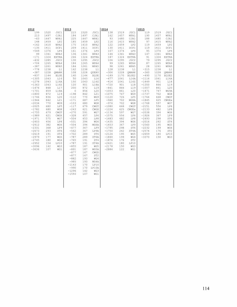
114
2012
199 1520 JGC1
213 1497 CJA1
-63 1447 WPA1
148 1459 LP2
-162 1410 WPA2
-135 1411 DCP1
-549 1376 LP4
99 1341 WPA3
-171 1324 EXTRA
-432 1285 JGC2
-704 1265 WPA4
-387 1261 WPA5
-778 1238 L1
-387 1228 QMARK
-837 1144 BLUE
-1305 1043 L16
-1278 1043 L16A
-1363 1043 L16Z
-1476 848 L17
-1701 859 L18A
-1800 872 L19
-1746 836 L20
-1944 842 L21
-2034 770 WG9
-2025 680 LP5
-1782 680 WG8
-1755 679 CWGT
-1989 621 CWGX
-1971 575 WG7
-2403 456 LP8
-2412 382 WG6
-2331 368 LP9
-2673 293 ST6
-2619 191 ST4
-2979 177 WG5
-2745 180 WG4
-2952 154 LP10
-3096 142 WG3
-3636 107 WG1
2013
215 1520 JGC1
184 1497 CJA1
225 1447 WPA1
185 1459 LP2
175 1410 WPA2
209 1411 DCP1
161 1376 LP4
136 1341 WPA3
246 1324 EXTRA
130 1295 JGC2
184 1265 WPA4
184 1261 WPA5
162 1238 L1
108 1228 QUERY
140 1144 BLUE
50 1043 L16
150 1043 L16Z
120 901 L18A
200 872 L19
0 856 L20
-198 842 L21
-112 770 WG9
-171 687 LP5
-103 680 WG8
-117 679 CWGT
-243 621 CWGX
-270 591 WG7
-328 457 LP6
-504 453 LP8
-531 394 WG6
-504 394 WG6A
-477 367 LP9
-562 367 LP9A
-702 289 ST6
-787 289 ST6A
-765 191 ST4
-787 191 ST4A
-855 187 WG5
-891 187 WG5A
-877 167 CWGD
-877 167 ST2
-882 193 WG4
-985 193 WG4A
-1143 170 LP10
-990 170 LP10A
-1296 142 WG3
-1593 107 WG1
2014
138 1519 JGC1
162 1457 WPA1
93 1480 CJA1
116 1415 WPA2
122 1459 LP2
130 1411 DCP1
107 1374 LP4
144 1341 WPA3
187 1324 EXTRA
106 1295 JGC2
99 1265 WPA4
98 1261 WPA5
128 1238 L1
-306 1228 QMARK
-189 1170 BLUE2
-477 1041 L16A
-414 1041 L16Z
-720 901 L18
-841 866 L19
-1053 861 L20
-1075 747 WG9
-1120 726 LP5
-940 702 WG8A
-976 702 WG8
-1080 668 CWGT
-1224 625 CWGEx
-1134 597 WG7
-1575 556 LP6
-1683 482 LP8
-1435 394 WG6
-1453 367 LP9
-1795 298 ST6
-1750 242 ST4A
-2124 195 WG5
-1840 199 WG4
-1876 176 ST2
-2421 180 LP10
-2178 150 WG3
-2884 122 WG1
2015
119 1519 JGC1
190 1457 WPA1
188 1480 CJA1
97 1415 WPA2
119 1459 LP2
119 1411 DCP1
95 1374 LP4
147 1341 WPA3
91 1324 EXTRA
79 1295 JGC2
87 1265 WPA4
28 1261 WPA5
-315 1238 L1
-360 1228 QMARK
-490 1170 BLUE2
-1116 1041 L16A
-1449 901 L18
-1350 866 L19
-1557 861 L20
-1471 747 WG9A
-1737 702 WG8
-1764 668 CWGT
-1845 625 CWGEx
-1768 597 WG7
-2151 556 LP6
-2133 482 LP8
-2038 394 WG6
-1926 367 LP9
-2493 298 ST6
-2016 242 ST4
-2560 195 WG5
-2232 199 WG4
-2574 176 ST2
-2659 180 LP10
-3370 150 WG3

115
APPENDIX 3: dGPS AND TEMPERATURE DATA 2012-2015
Dual-frequency GPS (dGPS) measurements were collected at White
Glacier between 2012 and 2015 for the purposes of velocity measurement
and comparison with earlier glacier dynamics studies conducted between
1960-1970. Details of the methods and findings of these earlier studies are
available in Müller and Iken [1973] and Iken [1974]. Contemporary
calculations of ice motion were acquired from differencing daily average
positions at the Upper (~870 m a.s.l.), Middle (~580 m a.s.l.), and Lower
(~370 m a.s.l.) dGPS stations at the same geographic locations of the earlier
studies. The instrumentation and installation of the stations is shown in A3,
Figure 1, and described in Chapter 4, Section 4.4.2, which includes details
of the post-processing techniques using the Precise Point Positioning (PPP) tool provided by Natural
Resources Canada: http://webapp.geod.nrcan.gc.ca/geod/tools-outils/ppp.php
The following Appendix provides tables of dGPS measurements of daily position, velocity, and
temperature, as well as their associated errors for each station for a given year. The daily mean Easting
(E), Northing (N), and Elevation (Z) is derived from the average of 24 hours of position measurements
(collected on a 15 s sampling interval) from 00h00 to 23h59, such that the daily mean position is centered
on noon (12h00) for a given day of year (DOY). The standard deviations of these E, N, and Z positions
(noted as E_std, N_std, and Z_std) are provided and incorporate both instrument error and the
displacement over the course of one day. The daily velocity down-glacier (Vx) is calculated from the slope
of a linear regression through the down-glacier displacement and sample time. The associated error
(Vx_err) is the root-mean square error incorporating the standard deviations of E and N. Daily mean
temperatures (T) were calculated from hourly measurements by shielded HOBO-U23 temperature/relative
humidity loggers. In instances where loggers failed or were not yet installed, T was modelled using daily
temperature lapse-rates derived from two automatic weather stations at the glacier terminus and an upper
nunatak. The final column in the tables provided (*) indicates whether the temperature values are based
upon this model (1) or observation (2). In 2012 the middle dGPS was initially programmed to collect
positions every 15 s for 1 hour between 12h00 and 13h00 local time daily. In this case, E, N, Z are
calculated from the mean of 1 hour of observation, and similarly for their standard deviations. Vx is
derived from the displacement between daily mean positions and therefore the first DOY with
observations does not have corresponding Vx or Vx_err values. Coordinates are in NAD83 UTM zone
15N and elevations are given in the Canadian Geodetic Vertical Datum (CGVD28_HTv2.0).
A3 Figure 1. dGPS station located at the
Lower station (~370 m a.s.l.), July 2014.
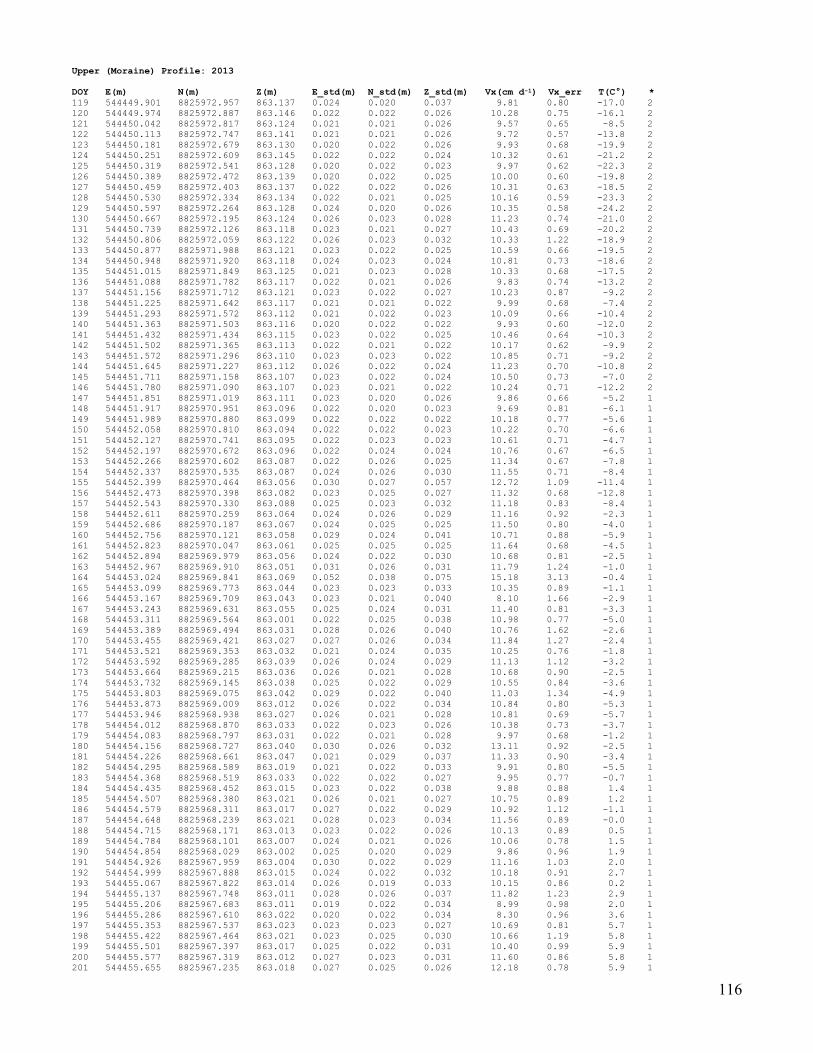
116
Upper (Moraine) Profile: 2013
DOY E(m) N(m) Z(m) E_std(m) N_std(m) Z_std(m) Vx(cm d-1) Vx_err T(C°) *
119 544449.901 8825972.957 863.137 0.024 0.020 0.037 9.81 0.80 -17.0 2
120 544449.974 8825972.887 863.146 0.022 0.022 0.026 10.28 0.75 -16.1 2
121 544450.042 8825972.817 863.124 0.021 0.021 0.026 9.57 0.65 -8.5 2
122 544450.113 8825972.747 863.141 0.021 0.021 0.026 9.72 0.57 -13.8 2
123 544450.181 8825972.679 863.130 0.020 0.022 0.026 9.93 0.68 -19.9 2
124 544450.251 8825972.609 863.145 0.022 0.022 0.024 10.32 0.61 -21.2 2
125 544450.319 8825972.541 863.128 0.020 0.022 0.023 9.97 0.62 -22.3 2
126 544450.389 8825972.472 863.139 0.020 0.022 0.025 10.00 0.60 -19.8 2
127 544450.459 8825972.403 863.137 0.022 0.022 0.026 10.31 0.63 -18.5 2
128 544450.530 8825972.334 863.134 0.022 0.021 0.025 10.16 0.59 -23.3 2
129 544450.597 8825972.264 863.128 0.024 0.020 0.026 10.35 0.58 -24.2 2
130 544450.667 8825972.195 863.124 0.026 0.023 0.028 11.23 0.74 -21.0 2
131 544450.739 8825972.126 863.118 0.023 0.021 0.027 10.43 0.69 -20.2 2
132 544450.806 8825972.059 863.122 0.026 0.023 0.032 10.33 1.22 -18.9 2
133 544450.877 8825971.988 863.121 0.023 0.022 0.025 10.59 0.66 -19.5 2
134 544450.948 8825971.920 863.118 0.024 0.023 0.024 10.81 0.73 -18.6 2
135 544451.015 8825971.849 863.125 0.021 0.023 0.028 10.33 0.68 -17.5 2
136 544451.088 8825971.782 863.117 0.022 0.021 0.026 9.83 0.74 -13.2 2
137 544451.156 8825971.712 863.121 0.023 0.022 0.027 10.23 0.87 -9.2 2
138 544451.225 8825971.642 863.117 0.021 0.021 0.022 9.99 0.68 -7.4 2
139 544451.293 8825971.572 863.112 0.021 0.022 0.023 10.09 0.66 -10.4 2
140 544451.363 8825971.503 863.116 0.020 0.022 0.022 9.93 0.60 -12.0 2
141 544451.432 8825971.434 863.115 0.023 0.022 0.025 10.46 0.64 -10.3 2
142 544451.502 8825971.365 863.113 0.022 0.021 0.022 10.17 0.62 -9.9 2
143 544451.572 8825971.296 863.110 0.023 0.023 0.022 10.85 0.71 -9.2 2
144 544451.645 8825971.227 863.112 0.026 0.022 0.024 11.23 0.70 -10.8 2
145 544451.711 8825971.158 863.107 0.023 0.022 0.024 10.50 0.73 -7.0 2
146 544451.780 8825971.090 863.107 0.023 0.021 0.022 10.24 0.71 -12.2 2
147 544451.851 8825971.019 863.111 0.023 0.020 0.026 9.86 0.66 -5.2 1
148 544451.917 8825970.951 863.096 0.022 0.020 0.023 9.69 0.81 -6.1 1
149 544451.989 8825970.880 863.099 0.022 0.022 0.022 10.18 0.77 -5.6 1
150 544452.058 8825970.810 863.094 0.022 0.022 0.023 10.22 0.70 -6.6 1
151 544452.127 8825970.741 863.095 0.022 0.023 0.023 10.61 0.71 -4.7 1
152 544452.197 8825970.672 863.096 0.022 0.024 0.024 10.76 0.67 -6.5 1
153 544452.266 8825970.602 863.087 0.022 0.026 0.025 11.34 0.67 -7.8 1
154 544452.337 8825970.535 863.087 0.024 0.026 0.030 11.55 0.71 -8.4 1
155 544452.399 8825970.464 863.056 0.030 0.027 0.057 12.72 1.09 -11.4 1
156 544452.473 8825970.398 863.082 0.023 0.025 0.027 11.32 0.68 -12.8 1
157 544452.543 8825970.330 863.088 0.025 0.023 0.032 11.18 0.83 -8.4 1
158 544452.611 8825970.259 863.064 0.024 0.026 0.029 11.16 0.92 -2.3 1
159 544452.686 8825970.187 863.067 0.024 0.025 0.025 11.50 0.80 -4.0 1
160 544452.756 8825970.121 863.058 0.029 0.024 0.041 10.71 0.88 -5.9 1
161 544452.823 8825970.047 863.061 0.025 0.025 0.025 11.64 0.68 -4.5 1
162 544452.894 8825969.979 863.056 0.024 0.022 0.030 10.68 0.81 -2.5 1
163 544452.967 8825969.910 863.051 0.031 0.026 0.031 11.79 1.24 -1.0 1
164 544453.024 8825969.841 863.069 0.052 0.038 0.075 15.18 3.13 -0.4 1
165 544453.099 8825969.773 863.044 0.023 0.023 0.033 10.35 0.89 -1.1 1
166 544453.167 8825969.709 863.043 0.023 0.021 0.040 8.10 1.66 -2.9 1
167 544453.243 8825969.631 863.055 0.025 0.024 0.031 11.40 0.81 -3.3 1
168 544453.311 8825969.564 863.001 0.022 0.025 0.038 10.98 0.77 -5.0 1
169 544453.389 8825969.494 863.031 0.028 0.026 0.040 10.76 1.62 -2.6 1
170 544453.455 8825969.421 863.027 0.027 0.026 0.034 11.84 1.27 -2.4 1
171 544453.521 8825969.353 863.032 0.021 0.024 0.035 10.25 0.76 -1.8 1
172 544453.592 8825969.285 863.039 0.026 0.024 0.029 11.13 1.12 -3.2 1
173 544453.664 8825969.215 863.036 0.026 0.021 0.028 10.68 0.90 -2.5 1
174 544453.732 8825969.145 863.038 0.025 0.022 0.029 10.55 0.84 -3.6 1
175 544453.803 8825969.075 863.042 0.029 0.022 0.040 11.03 1.34 -4.9 1
176 544453.873 8825969.009 863.012 0.026 0.022 0.034 10.84 0.80 -5.3 1
177 544453.946 8825968.938 863.027 0.026 0.021 0.028 10.81 0.69 -5.7 1
178 544454.012 8825968.870 863.033 0.022 0.023 0.026 10.38 0.73 -3.7 1
179 544454.083 8825968.797 863.031 0.022 0.021 0.028 9.97 0.68 -1.2 1
180 544454.156 8825968.727 863.040 0.030 0.026 0.032 13.11 0.92 -2.5 1
181 544454.226 8825968.661 863.047 0.021 0.029 0.037 11.33 0.90 -3.4 1
182 544454.295 8825968.589 863.019 0.021 0.022 0.033 9.91 0.80 -5.5 1
183 544454.368 8825968.519 863.033 0.022 0.022 0.027 9.95 0.77 -0.7 1
184 544454.435 8825968.452 863.015 0.023 0.022 0.038 9.88 0.88 1.4 1
185 544454.507 8825968.380 863.021 0.026 0.021 0.027 10.75 0.89 1.2 1
186 544454.579 8825968.311 863.017 0.027 0.022 0.029 10.92 1.12 -1.1 1
187 544454.648 8825968.239 863.021 0.028 0.023 0.034 11.56 0.89 -0.0 1
188 544454.715 8825968.171 863.013 0.023 0.022 0.026 10.13 0.89 0.5 1
189 544454.784 8825968.101 863.007 0.024 0.021 0.026 10.06 0.78 1.5 1
190 544454.854 8825968.029 863.002 0.025 0.020 0.029 9.86 0.96 1.9 1
191 544454.926 8825967.959 863.004 0.030 0.022 0.029 11.16 1.03 2.0 1
192 544454.999 8825967.888 863.015 0.024 0.022 0.032 10.18 0.91 2.7 1
193 544455.067 8825967.822 863.014 0.026 0.019 0.033 10.15 0.86 0.2 1
194 544455.137 8825967.748 863.011 0.028 0.026 0.037 11.82 1.23 2.9 1
195 544455.206 8825967.683 863.011 0.019 0.022 0.034 8.99 0.98 2.0 1
196 544455.286 8825967.610 863.022 0.020 0.022 0.034 8.30 0.96 3.6 1
197 544455.353 8825967.537 863.023 0.023 0.023 0.027 10.69 0.81 5.7 1
198 544455.422 8825967.464 863.021 0.023 0.025 0.030 10.66 1.19 5.8 1
199 544455.501 8825967.397 863.017 0.025 0.022 0.031 10.40 0.99 5.9 1
200 544455.577 8825967.319 863.012 0.027 0.023 0.031 11.60 0.86 5.8 1
201 544455.655 8825967.235 863.018 0.027 0.025 0.026 12.18 0.78 5.9 1
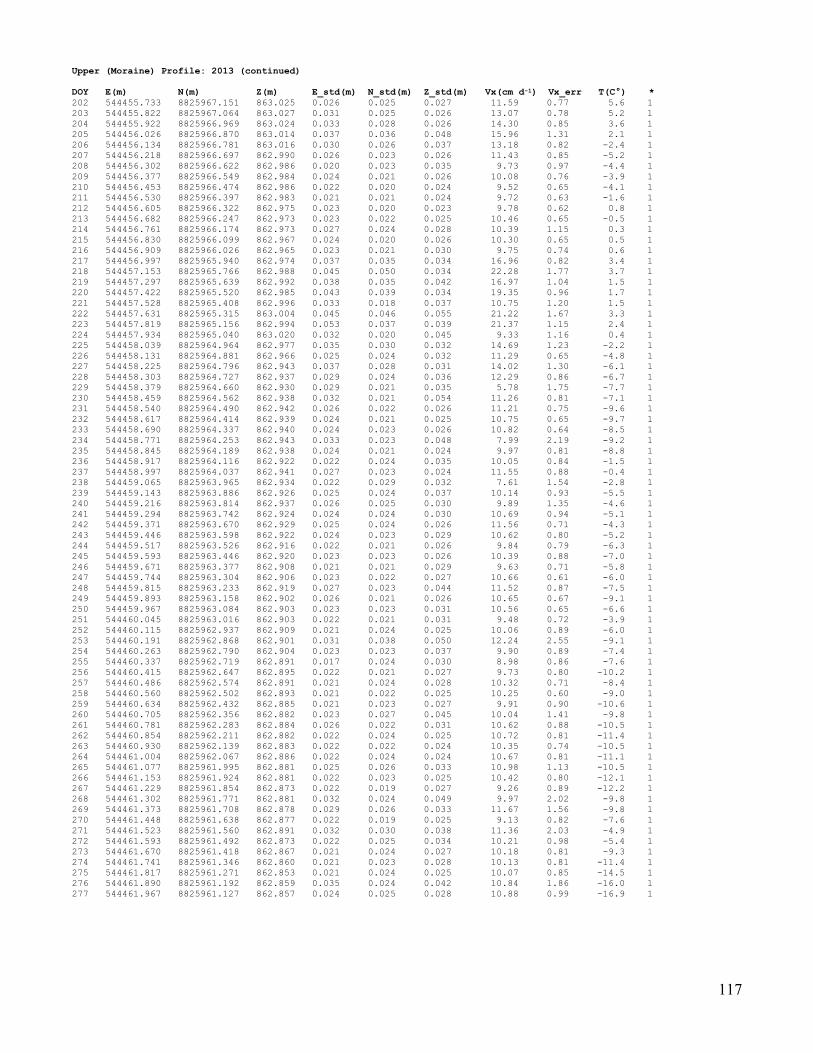
117
Upper (Moraine) Profile: 2013 (continued)
DOY E(m) N(m) Z(m) E_std(m) N_std(m) Z_std(m) Vx(cm d-1) Vx_err T(C°) *
202 544455.733 8825967.151 863.025 0.026 0.025 0.027 11.59 0.77 5.6 1
203 544455.822 8825967.064 863.027 0.031 0.025 0.026 13.07 0.78 5.2 1
204 544455.922 8825966.969 863.024 0.033 0.028 0.026 14.30 0.85 3.6 1
205 544456.026 8825966.870 863.014 0.037 0.036 0.048 15.96 1.31 2.1 1
206 544456.134 8825966.781 863.016 0.030 0.026 0.037 13.18 0.82 -2.4 1
207 544456.218 8825966.697 862.990 0.026 0.023 0.026 11.43 0.85 -5.2 1
208 544456.302 8825966.622 862.986 0.020 0.023 0.035 9.73 0.97 -4.4 1
209 544456.377 8825966.549 862.984 0.024 0.021 0.026 10.08 0.76 -3.9 1
210 544456.453 8825966.474 862.986 0.022 0.020 0.024 9.52 0.65 -4.1 1
211 544456.530 8825966.397 862.983 0.021 0.021 0.024 9.72 0.63 -1.6 1
212 544456.605 8825966.322 862.975 0.023 0.020 0.023 9.78 0.62 0.8 1
213 544456.682 8825966.247 862.973 0.023 0.022 0.025 10.46 0.65 -0.5 1
214 544456.761 8825966.174 862.973 0.027 0.024 0.028 10.39 1.15 0.3 1
215 544456.830 8825966.099 862.967 0.024 0.020 0.026 10.30 0.65 0.5 1
216 544456.909 8825966.026 862.965 0.023 0.021 0.030 9.75 0.74 0.6 1
217 544456.997 8825965.940 862.974 0.037 0.035 0.034 16.96 0.82 3.4 1
218 544457.153 8825965.766 862.988 0.045 0.050 0.034 22.28 1.77 3.7 1
219 544457.297 8825965.639 862.992 0.038 0.035 0.042 16.97 1.04 1.5 1
220 544457.422 8825965.520 862.985 0.043 0.039 0.034 19.35 0.96 1.7 1
221 544457.528 8825965.408 862.996 0.033 0.018 0.037 10.75 1.20 1.5 1
222 544457.631 8825965.315 863.004 0.045 0.046 0.055 21.22 1.67 3.3 1
223 544457.819 8825965.156 862.994 0.053 0.037 0.039 21.37 1.15 2.4 1
224 544457.934 8825965.040 863.020 0.032 0.020 0.045 9.33 1.16 0.4 1
225 544458.039 8825964.964 862.977 0.035 0.030 0.032 14.69 1.23 -2.2 1
226 544458.131 8825964.881 862.966 0.025 0.024 0.032 11.29 0.65 -4.8 1
227 544458.225 8825964.796 862.943 0.037 0.028 0.031 14.02 1.30 -6.1 1
228 544458.303 8825964.727 862.937 0.029 0.024 0.036 12.29 0.86 -6.7 1
229 544458.379 8825964.660 862.930 0.029 0.021 0.035 5.78 1.75 -7.7 1
230 544458.459 8825964.562 862.938 0.032 0.021 0.054 11.26 0.81 -7.1 1
231 544458.540 8825964.490 862.942 0.026 0.022 0.026 11.21 0.75 -9.6 1
232 544458.617 8825964.414 862.939 0.024 0.021 0.025 10.75 0.65 -9.7 1
233 544458.690 8825964.337 862.940 0.024 0.023 0.026 10.82 0.64 -8.5 1
234 544458.771 8825964.253 862.943 0.033 0.023 0.048 7.99 2.19 -9.2 1
235 544458.845 8825964.189 862.938 0.024 0.021 0.024 9.97 0.81 -8.8 1
236 544458.917 8825964.116 862.922 0.022 0.024 0.035 10.05 0.84 -1.5 1
237 544458.997 8825964.037 862.941 0.027 0.023 0.024 11.55 0.88 -0.4 1
238 544459.065 8825963.965 862.934 0.022 0.029 0.032 7.61 1.54 -2.8 1
239 544459.143 8825963.886 862.926 0.025 0.024 0.037 10.14 0.93 -5.5 1
240 544459.216 8825963.814 862.937 0.026 0.025 0.030 9.89 1.35 -4.6 1
241 544459.294 8825963.742 862.924 0.024 0.024 0.030 10.69 0.94 -5.1 1
242 544459.371 8825963.670 862.929 0.025 0.024 0.026 11.56 0.71 -4.3 1
243 544459.446 8825963.598 862.922 0.024 0.023 0.029 10.62 0.80 -5.2 1
244 544459.517 8825963.526 862.916 0.022 0.021 0.026 9.84 0.79 -6.3 1
245 544459.593 8825963.446 862.920 0.023 0.023 0.026 10.39 0.88 -7.0 1
246 544459.671 8825963.377 862.908 0.021 0.021 0.029 9.63 0.71 -5.8 1
247 544459.744 8825963.304 862.906 0.023 0.022 0.027 10.66 0.61 -6.0 1
248 544459.815 8825963.233 862.919 0.027 0.023 0.044 11.52 0.87 -7.5 1
249 544459.893 8825963.158 862.902 0.026 0.021 0.026 10.65 0.67 -9.1 1
250 544459.967 8825963.084 862.903 0.023 0.023 0.031 10.56 0.65 -6.6 1
251 544460.045 8825963.016 862.903 0.022 0.021 0.031 9.48 0.72 -3.9 1
252 544460.115 8825962.937 862.909 0.021 0.024 0.025 10.06 0.89 -6.0 1
253 544460.191 8825962.868 862.901 0.031 0.038 0.050 12.24 2.55 -9.1 1
254 544460.263 8825962.790 862.904 0.023 0.023 0.037 9.90 0.89 -7.4 1
255 544460.337 8825962.719 862.891 0.017 0.024 0.030 8.98 0.86 -7.6 1
256 544460.415 8825962.647 862.895 0.022 0.021 0.027 9.73 0.80 -10.2 1
257 544460.486 8825962.574 862.891 0.021 0.024 0.028 10.32 0.71 -8.4 1
258 544460.560 8825962.502 862.893 0.021 0.022 0.025 10.25 0.60 -9.0 1
259 544460.634 8825962.432 862.885 0.021 0.023 0.027 9.91 0.90 -10.6 1
260 544460.705 8825962.356 862.882 0.023 0.027 0.045 10.04 1.41 -9.8 1
261 544460.781 8825962.283 862.884 0.026 0.022 0.031 10.62 0.88 -10.5 1
262 544460.854 8825962.211 862.882 0.022 0.024 0.025 10.72 0.81 -11.4 1
263 544460.930 8825962.139 862.883 0.022 0.022 0.024 10.35 0.74 -10.5 1
264 544461.004 8825962.067 862.886 0.022 0.024 0.024 10.67 0.81 -11.1 1
265 544461.077 8825961.995 862.881 0.025 0.026 0.033 10.98 1.13 -10.5 1
266 544461.153 8825961.924 862.881 0.022 0.023 0.025 10.42 0.80 -12.1 1
267 544461.229 8825961.854 862.873 0.022 0.019 0.027 9.26 0.89 -12.2 1
268 544461.302 8825961.771 862.881 0.032 0.024 0.049 9.97 2.02 -9.8 1
269 544461.373 8825961.708 862.878 0.029 0.026 0.033 11.67 1.56 -9.8 1
270 544461.448 8825961.638 862.877 0.022 0.019 0.025 9.13 0.82 -7.6 1
271 544461.523 8825961.560 862.891 0.032 0.030 0.038 11.36 2.03 -4.9 1
272 544461.593 8825961.492 862.873 0.022 0.025 0.034 10.21 0.98 -5.4 1
273 544461.670 8825961.418 862.867 0.021 0.024 0.027 10.18 0.81 -9.3 1
274 544461.741 8825961.346 862.860 0.021 0.023 0.028 10.13 0.81 -11.4 1
275 544461.817 8825961.271 862.853 0.021 0.024 0.025 10.07 0.85 -14.5 1
276 544461.890 8825961.192 862.859 0.035 0.024 0.042 10.84 1.86 -16.0 1
277 544461.967 8825961.127 862.857 0.024 0.025 0.028 10.88 0.99 -16.9 1
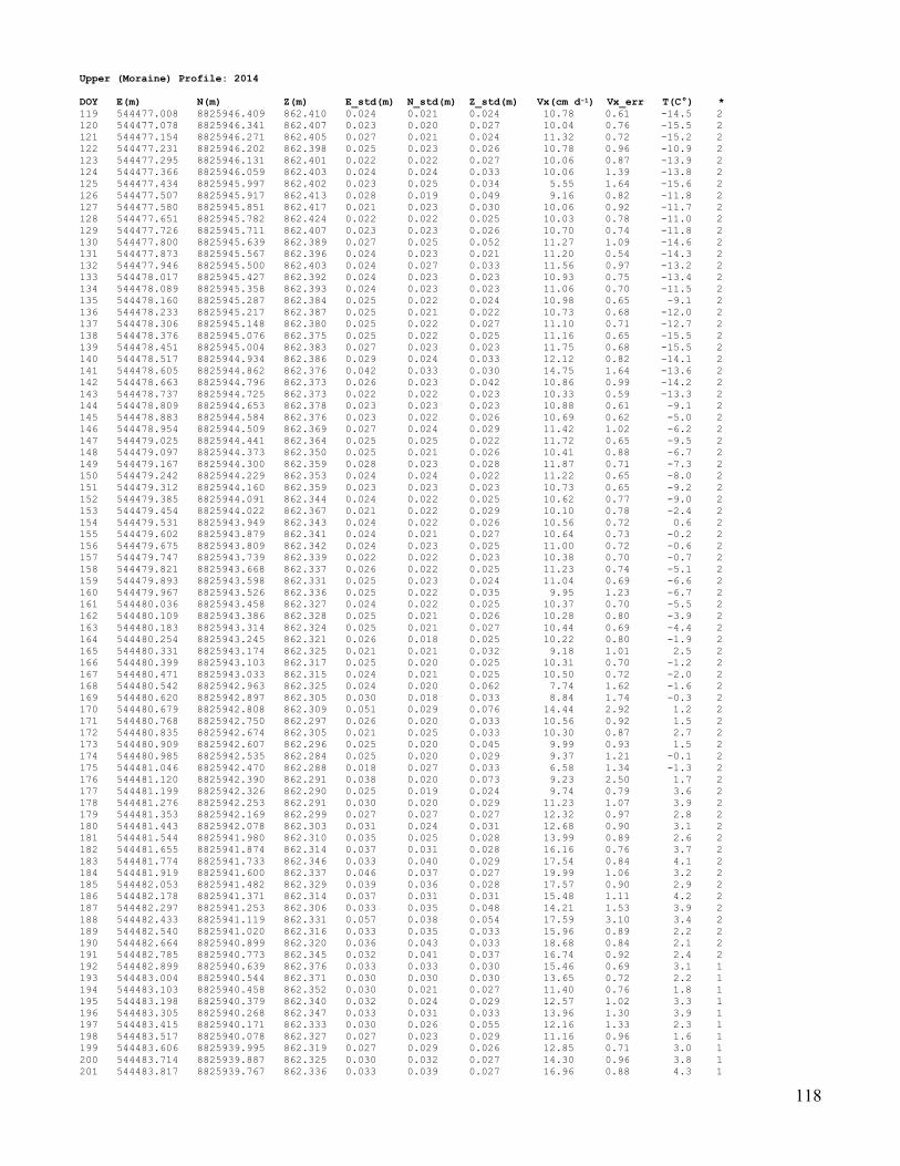
118
Upper (Moraine) Profile: 2014
DOY E(m) N(m) Z(m) E_std(m) N_std(m) Z_std(m) Vx(cm d-1) Vx_err T(C°) *
119 544477.008 8825946.409 862.410 0.024 0.021 0.024 10.78 0.61 -14.5 2
120 544477.078 8825946.341 862.407 0.023 0.020 0.027 10.04 0.76 -15.5 2
121 544477.154 8825946.271 862.405 0.027 0.021 0.024 11.32 0.72 -15.2 2
122 544477.231 8825946.202 862.398 0.025 0.023 0.026 10.78 0.96 -10.9 2
123 544477.295 8825946.131 862.401 0.022 0.022 0.027 10.06 0.87 -13.9 2
124 544477.366 8825946.059 862.403 0.024 0.024 0.033 10.06 1.39 -13.8 2
125 544477.434 8825945.997 862.402 0.023 0.025 0.034 5.55 1.64 -15.6 2
126 544477.507 8825945.917 862.413 0.028 0.019 0.049 9.16 0.82 -11.8 2
127 544477.580 8825945.851 862.417 0.021 0.023 0.030 10.06 0.92 -11.7 2
128 544477.651 8825945.782 862.424 0.022 0.022 0.025 10.03 0.78 -11.0 2
129 544477.726 8825945.711 862.407 0.023 0.023 0.026 10.70 0.74 -11.8 2
130 544477.800 8825945.639 862.389 0.027 0.025 0.052 11.27 1.09 -14.6 2
131 544477.873 8825945.567 862.396 0.024 0.023 0.021 11.20 0.54 -14.3 2
132 544477.946 8825945.500 862.403 0.024 0.027 0.033 11.56 0.97 -13.2 2
133 544478.017 8825945.427 862.392 0.024 0.023 0.023 10.93 0.75 -13.4 2
134 544478.089 8825945.358 862.393 0.024 0.023 0.023 11.06 0.70 -11.5 2
135 544478.160 8825945.287 862.384 0.025 0.022 0.024 10.98 0.65 -9.1 2
136 544478.233 8825945.217 862.387 0.025 0.021 0.022 10.73 0.68 -12.0 2
137 544478.306 8825945.148 862.380 0.025 0.022 0.027 11.10 0.71 -12.7 2
138 544478.376 8825945.076 862.375 0.025 0.022 0.025 11.16 0.65 -15.5 2
139 544478.451 8825945.004 862.383 0.027 0.023 0.023 11.75 0.68 -15.5 2
140 544478.517 8825944.934 862.386 0.029 0.024 0.033 12.12 0.82 -14.1 2
141 544478.605 8825944.862 862.376 0.042 0.033 0.030 14.75 1.64 -13.6 2
142 544478.663 8825944.796 862.373 0.026 0.023 0.042 10.86 0.99 -14.2 2
143 544478.737 8825944.725 862.373 0.022 0.022 0.023 10.33 0.59 -13.3 2
144 544478.809 8825944.653 862.378 0.023 0.023 0.023 10.88 0.61 -9.1 2
145 544478.883 8825944.584 862.376 0.023 0.022 0.026 10.69 0.62 -5.0 2
146 544478.954 8825944.509 862.369 0.027 0.024 0.029 11.42 1.02 -6.2 2
147 544479.025 8825944.441 862.364 0.025 0.025 0.022 11.72 0.65 -9.5 2
148 544479.097 8825944.373 862.350 0.025 0.021 0.026 10.41 0.88 -6.7 2
149 544479.167 8825944.300 862.359 0.028 0.023 0.028 11.87 0.71 -7.3 2
150 544479.242 8825944.229 862.353 0.024 0.024 0.022 11.22 0.65 -8.0 2
151 544479.312 8825944.160 862.359 0.023 0.023 0.023 10.73 0.65 -9.2 2
152 544479.385 8825944.091 862.344 0.024 0.022 0.025 10.62 0.77 -9.0 2
153 544479.454 8825944.022 862.367 0.021 0.022 0.029 10.10 0.78 -2.4 2
154 544479.531 8825943.949 862.343 0.024 0.022 0.026 10.56 0.72 0.6 2
155 544479.602 8825943.879 862.341 0.024 0.021 0.027 10.64 0.73 -0.2 2
156 544479.675 8825943.809 862.342 0.024 0.023 0.025 11.00 0.72 -0.6 2
157 544479.747 8825943.739 862.339 0.022 0.022 0.023 10.38 0.70 -0.7 2
158 544479.821 8825943.668 862.337 0.026 0.022 0.025 11.23 0.74 -5.1 2
159 544479.893 8825943.598 862.331 0.025 0.023 0.024 11.04 0.69 -6.6 2
160 544479.967 8825943.526 862.336 0.025 0.022 0.035 9.95 1.23 -6.7 2
161 544480.036 8825943.458 862.327 0.024 0.022 0.025 10.37 0.70 -5.5 2
162 544480.109 8825943.386 862.328 0.025 0.021 0.026 10.28 0.80 -3.9 2
163 544480.183 8825943.314 862.324 0.025 0.021 0.027 10.44 0.69 -4.4 2
164 544480.254 8825943.245 862.321 0.026 0.018 0.025 10.22 0.80 -1.9 2
165 544480.331 8825943.174 862.325 0.021 0.021 0.032 9.18 1.01 2.5 2
166 544480.399 8825943.103 862.317 0.025 0.020 0.025 10.31 0.70 -1.2 2
167 544480.471 8825943.033 862.315 0.024 0.021 0.025 10.50 0.72 -2.0 2
168 544480.542 8825942.963 862.325 0.024 0.020 0.062 7.74 1.62 -1.6 2
169 544480.620 8825942.897 862.305 0.030 0.018 0.033 8.84 1.74 -0.3 2
170 544480.679 8825942.808 862.309 0.051 0.029 0.076 14.44 2.92 1.2 2
171 544480.768 8825942.750 862.297 0.026 0.020 0.033 10.56 0.92 1.5 2
172 544480.835 8825942.674 862.305 0.021 0.025 0.033 10.30 0.87 2.7 2
173 544480.909 8825942.607 862.296 0.025 0.020 0.045 9.99 0.93 1.5 2
174 544480.985 8825942.535 862.284 0.025 0.020 0.029 9.37 1.21 -0.1 2
175 544481.046 8825942.470 862.288 0.018 0.027 0.033 6.58 1.34 -1.3 2
176 544481.120 8825942.390 862.291 0.038 0.020 0.073 9.23 2.50 1.7 2
177 544481.199 8825942.326 862.290 0.025 0.019 0.024 9.74 0.79 3.6 2
178 544481.276 8825942.253 862.291 0.030 0.020 0.029 11.23 1.07 3.9 2
179 544481.353 8825942.169 862.299 0.027 0.027 0.027 12.32 0.97 2.8 2
180 544481.443 8825942.078 862.303 0.031 0.024 0.031 12.68 0.90 3.1 2
181 544481.544 8825941.980 862.310 0.035 0.025 0.028 13.99 0.89 2.6 2
182 544481.655 8825941.874 862.314 0.037 0.031 0.028 16.16 0.76 3.7 2
183 544481.774 8825941.733 862.346 0.033 0.040 0.029 17.54 0.84 4.1 2
184 544481.919 8825941.600 862.337 0.046 0.037 0.027 19.99 1.06 3.2 2
185 544482.053 8825941.482 862.329 0.039 0.036 0.028 17.57 0.90 2.9 2
186 544482.178 8825941.371 862.314 0.037 0.031 0.031 15.48 1.11 4.2 2
187 544482.297 8825941.253 862.306 0.033 0.035 0.048 14.21 1.53 3.9 2
188 544482.433 8825941.119 862.331 0.057 0.038 0.054 17.59 3.10 3.4 2
189 544482.540 8825941.020 862.316 0.033 0.035 0.033 15.96 0.89 2.2 2
190 544482.664 8825940.899 862.320 0.036 0.043 0.033 18.68 0.84 2.1 2
191 544482.785 8825940.773 862.345 0.032 0.041 0.037 16.74 0.92 2.4 2
192 544482.899 8825940.639 862.376 0.033 0.033 0.030 15.46 0.69 3.1 1
193 544483.004 8825940.544 862.371 0.030 0.030 0.030 13.65 0.72 2.2 1
194 544483.103 8825940.458 862.352 0.030 0.021 0.027 11.40 0.76 1.8 1
195 544483.198 8825940.379 862.340 0.032 0.024 0.029 12.57 1.02 3.3 1
196 544483.305 8825940.268 862.347 0.033 0.031 0.033 13.96 1.30 3.9 1
197 544483.415 8825940.171 862.333 0.030 0.026 0.055 12.16 1.33 2.3 1
198 544483.517 8825940.078 862.327 0.027 0.023 0.029 11.16 0.96 1.6 1
199 544483.606 8825939.995 862.319 0.027 0.029 0.026 12.85 0.71 3.0 1
200 544483.714 8825939.887 862.325 0.030 0.032 0.027 14.30 0.96 3.8 1
201 544483.817 8825939.767 862.336 0.033 0.039 0.027 16.96 0.88 4.3 1

119
Upper (Moraine) Profile: 2014 (continued)
DOY E(m) N(m) Z(m) E_std(m) N_std(m) Z_std(m) Vx(cm d-1) Vx_err T(C°) *
202 544483.933 8825939.655 862.337 0.033 0.034 0.029 15.76 0.87 3.4 1
203 544484.037 8825939.571 862.320 0.030 0.018 0.031 10.62 0.86 1.6 1
204 544484.143 8825939.490 862.292 0.037 0.020 0.031 11.48 1.20 -3.5 1
205 544484.242 8825939.410 862.272 0.029 0.024 0.029 12.45 0.65 -1.3 1
206 544484.328 8825939.327 862.262 0.025 0.022 0.027 10.29 0.67 2.9 1
207 544484.414 8825939.244 862.259 0.029 0.023 0.027 11.58 0.74 1.2 1
208 544484.506 8825939.160 862.249 0.027 0.021 0.031 11.16 0.64 -0.7 1
209 544484.590 8825939.071 862.244 0.027 0.026 0.030 12.23 0.91 -0.8 1
210 544484.673 8825938.993 862.242 0.029 0.024 0.040 11.43 1.21 0.6 1
211 544484.753 8825938.919 862.234 0.025 0.025 0.024 11.63 0.69 2.4 1
212 544484.844 8825938.829 862.245 0.024 0.028 0.029 11.79 0.69 3.0 1
213 544484.957 8825938.717 862.243 0.035 0.027 0.031 14.56 0.78 3.7 1
214 544485.071 8825938.598 862.262 0.042 0.054 0.047 21.99 1.81 4.9 1
215 544485.233 8825938.461 862.228 0.039 0.039 0.026 18.56 0.70 0.5 1
216 544485.345 8825938.357 862.230 0.026 0.024 0.027 11.43 0.77 1.4 1
217 544485.432 8825938.280 862.211 0.027 0.024 0.026 11.97 0.83 2.6 1
218 544485.526 8825938.193 862.205 0.027 0.026 0.026 12.27 0.81 3.3 1
219 544485.632 8825938.097 862.211 0.036 0.031 0.026 16.21 0.74 4.4 1
220 544485.749 8825937.995 862.203 0.034 0.033 0.031 15.78 1.01 5.0 1
221 544485.864 8825937.894 862.198 0.033 0.032 0.035 14.95 1.34 5.2 1
222 544485.965 8825937.808 862.193 0.028 0.026 0.034 12.40 0.97 2.6 1
223 544486.054 8825937.727 862.179 0.029 0.026 0.025 12.87 0.63 0.7 1
224 544486.145 8825937.640 862.184 0.036 0.025 0.033 12.80 1.64 0.8 1
225 544486.229 8825937.565 862.173 0.025 0.026 0.027 11.54 0.85 2.6 1
226 544486.319 8825937.487 862.179 0.022 0.026 0.032 10.80 1.09 1.0 1
227 544486.397 8825937.406 862.167 0.025 0.025 0.025 11.58 0.65 -0.3 1
228 544486.482 8825937.331 862.151 0.023 0.025 0.028 10.99 0.87 0.4 1
229 544486.570 8825937.251 862.155 0.028 0.021 0.028 11.09 0.92 -0.2 1
230 544486.635 8825937.178 862.164 0.044 0.036 0.065 16.14 2.13 -1.4 1
231 544486.727 8825937.101 862.146 0.023 0.022 0.028 10.24 0.82 0.5 1
232 544486.805 8825937.021 862.152 0.025 0.019 0.034 9.59 0.91 1.5 1
233 544486.889 8825936.948 862.143 0.027 0.022 0.048 9.55 1.37 -0.7 1
234 544486.962 8825936.874 862.141 0.020 0.022 0.031 9.56 0.85 -2.8 1
235 544487.035 8825936.804 862.133 0.020 0.020 0.023 9.25 0.60 -2.5 1
236 544487.116 8825936.729 862.133 0.026 0.022 0.025 10.99 0.77 -1.1 1
237 544487.191 8825936.655 862.138 0.022 0.024 0.023 10.72 0.61 -0.9 1
238 544487.268 8825936.582 862.140 0.018 0.023 0.023 9.43 0.72 -0.8 1
239 544487.339 8825936.511 862.128 0.020 0.023 0.031 9.32 1.03 -4.2 1
240 544487.418 8825936.438 862.128 0.021 0.023 0.026 9.66 0.77 -2.5 1
241 544487.492 8825936.368 862.119 0.022 0.023 0.028 9.75 1.09 -0.8 1
242 544487.572 8825936.291 862.130 0.021 0.022 0.022 9.80 0.74 1.0 1
243 544487.648 8825936.217 862.126 0.023 0.028 0.029 11.23 0.98 0.9 1
244 544487.726 8825936.146 862.119 0.019 0.023 0.024 9.41 0.72 0.0 1
245 544487.800 8825936.071 862.120 0.018 0.023 0.022 9.20 0.87 -0.6 1
246 544487.878 8825935.997 862.122 0.022 0.022 0.023 10.10 0.66 -1.3 1
247 544487.950 8825935.924 862.123 0.018 0.024 0.030 9.34 0.87 -1.1 1
248 544488.025 8825935.853 862.114 0.019 0.022 0.028 9.25 0.72 -2.5 1
249 544488.102 8825935.780 862.112 0.020 0.021 0.023 9.29 0.73 -1.9 1
250 544488.176 8825935.708 862.110 0.021 0.024 0.023 10.34 0.82 -4.1 1
251 544488.252 8825935.637 862.122 0.018 0.025 0.036 9.29 1.15 -4.3 1
252 544488.326 8825935.563 862.098 0.021 0.027 0.027 10.75 1.21 -7.9 1
253 544488.405 8825935.490 862.102 0.022 0.023 0.024 10.51 0.96 -9.4 1
254 544488.478 8825935.418 862.098 0.019 0.024 0.023 9.51 1.00 -9.7 1
255 544488.554 8825935.345 862.099 0.023 0.024 0.026 10.63 0.91 -9.0 1
256 544488.634 8825935.271 862.077 0.024 0.023 0.032 10.59 0.95 -8.3 1
257 544488.707 8825935.197 862.087 0.023 0.028 0.039 11.04 1.29 -9.1 1
258 544488.782 8825935.128 862.089 0.022 0.024 0.026 10.39 0.96 -7.6 1
259 544488.858 8825935.057 862.088 0.022 0.023 0.023 9.69 1.06 -8.9 1
260 544488.931 8825934.985 862.088 0.020 0.023 0.022 9.57 0.98 -8.9 1
261 544489.005 8825934.914 862.086 0.016 0.023 0.024 8.52 1.04 -7.2 1
262 544489.088 8825934.841 862.088 0.017 0.026 0.025 9.26 0.97 -3.2 1
263 544489.158 8825934.768 862.078 0.020 0.027 0.025 10.86 0.74 -5.6 1
264 544489.233 8825934.695 862.085 0.024 0.024 0.025 11.00 0.74 -10.2 1
265 544489.305 8825934.624 862.078 0.022 0.023 0.028 10.48 0.75 -10.3 1
266 544489.379 8825934.552 862.074 0.023 0.026 0.023 11.14 0.85 -11.9 1
267 544489.457 8825934.482 862.065 0.020 0.025 0.028 10.34 0.75 -12.4 1
268 544489.531 8825934.406 862.070 0.024 0.024 0.025 11.08 0.83 -12.4 1
269 544489.607 8825934.334 862.069 0.024 0.025 0.028 11.03 0.96 -14.7 1
270 544489.682 8825934.263 862.067 0.023 0.023 0.024 10.51 0.87 -15.8 1
271 544489.756 8825934.191 862.064 0.024 0.025 0.024 10.94 1.01 -14.4 1
272 544489.834 8825934.117 862.064 0.027 0.028 0.027 12.10 1.10 -14.4 1
273 544489.905 8825934.050 862.058 0.026 0.025 0.027 11.06 1.14 -11.6 1
274 544489.993 8825933.970 862.053 0.024 0.025 0.028 11.02 0.73 -11.2 1
275 544490.065 8825933.895 862.055 0.023 0.022 0.025 11.66 1.09 -10.6 1
276 544490.136 8825933.827 862.055 0.021 0.022 0.026 10.90 0.86 -10.9 1

120
Upper (Moraine) Profile: 2015
DOY E(m) N(m) Z(m) E_std(m) N_std(m) Z_std(m) Vx(cm d-1) Vx_err T(C°) *
114 544504.950 8825921.528 860.774 0.023 0.022 0.022 10.70 0.58 -13.5 2
115 544505.019 8825921.459 860.781 0.020 0.021 0.027 9.22 0.82 -11.0 2
116 544505.097 8825921.387 860.781 0.023 0.020 0.025 10.01 0.71 -9.2 2
117 544505.167 8825921.319 860.777 0.025 0.023 0.026 11.10 0.64 -11.3 2
118 544505.241 8825921.250 860.771 0.025 0.021 0.024 10.76 0.53 -12.9 2
119 544505.313 8825921.180 860.769 0.024 0.021 0.024 10.72 0.65 -13.9 2
120 544505.384 8825921.110 860.764 0.025 0.022 0.025 11.23 0.60 -12.9 2
121 544505.456 8825921.042 860.765 0.024 0.023 0.026 10.79 0.64 -12.7 2
122 544505.529 8825920.972 860.758 0.026 0.022 0.025 11.33 0.68 -12.0 2
123 544505.601 8825920.903 860.754 0.026 0.021 0.027 11.04 0.69 -11.0 2
124 544505.674 8825920.832 860.753 0.024 0.022 0.025 10.89 0.56 -11.4 2
125 544505.746 8825920.766 860.751 0.022 0.022 0.025 10.24 0.78 -12.7 2
126 544505.820 8825920.692 860.748 0.025 0.022 0.026 10.98 0.67 -14.2 2
127 544505.893 8825920.625 860.749 0.026 0.021 0.024 11.11 0.69 -17.2 2
128 544505.965 8825920.554 860.742 0.024 0.022 0.025 10.88 0.65 -17.5 2
129 544506.039 8825920.484 860.742 0.026 0.023 0.025 11.28 0.83 -15.2 2
130 544506.111 8825920.415 860.751 0.025 0.025 0.033 11.55 0.85 -11.9 2
131 544506.175 8825920.346 860.735 0.035 0.029 0.057 13.12 1.97 -14.7 2
132 544506.256 8825920.274 860.736 0.027 0.024 0.024 11.95 0.73 -17.2 2
133 544506.328 8825920.206 860.733 0.023 0.025 0.024 11.22 0.64 -18.6 2
134 544506.401 8825920.132 860.724 0.027 0.025 0.032 11.98 0.75 -17.4 2
135 544506.475 8825920.064 860.709 0.026 0.029 0.029 12.76 0.81 -12.7 2
136 544506.547 8825919.995 860.730 0.023 0.024 0.025 11.15 0.76 -9.0 2
137 544506.618 8825919.927 860.732 0.023 0.023 0.027 10.68 0.83 -9.9 2
138 544506.694 8825919.858 860.720 0.027 0.021 0.032 10.93 1.04 -9.0 2
139 544506.764 8825919.789 860.719 0.026 0.023 0.031 11.27 0.84 -10.3 2
140 544506.836 8825919.718 860.725 0.025 0.022 0.031 10.92 0.75 -9.6 2
141 544506.910 8825919.649 860.704 0.026 0.022 0.024 11.12 0.79 -10.4 2
142 544506.982 8825919.579 860.702 0.025 0.023 0.029 11.07 0.68 -14.1 2
143 544507.056 8825919.504 860.692 0.027 0.026 0.028 12.33 0.83 -16.1 2
144 544507.129 8825919.437 860.688 0.025 0.025 0.025 11.33 0.80 -8.6 2
145 544507.202 8825919.370 860.680 0.023 0.019 0.033 9.12 1.19 -8.2 2
146 544507.272 8825919.298 860.692 0.030 0.023 0.032 12.35 0.92 -4.7 2
147 544507.348 8825919.226 860.685 0.026 0.023 0.025 11.35 0.76 -4.5 2
148 544507.422 8825919.158 860.697 0.025 0.023 0.030 11.12 0.69 -5.0 2
149 544507.489 8825919.091 860.683 0.029 0.028 0.029 12.36 1.53 -4.6 2
150 544507.565 8825919.018 860.680 0.025 0.022 0.026 10.80 0.79 -4.6 2
151 544507.639 8825918.950 860.679 0.026 0.022 0.029 11.00 0.87 -2.0 2
152 544507.708 8825918.879 860.672 0.028 0.024 0.025 11.69 1.19 -0.6 2
153 544507.782 8825918.805 860.673 0.025 0.022 0.025 11.02 0.65 -1.7 2
154 544507.853 8825918.740 860.671 0.031 0.027 0.024 12.66 1.43 -0.2 2
155 544507.931 8825918.666 860.668 0.027 0.021 0.023 11.11 0.65 -0.7 2
156 544508.007 8825918.596 860.669 0.028 0.022 0.023 11.63 0.71 -1.7 2
157 544508.081 8825918.528 860.668 0.030 0.025 0.028 11.93 1.41 -4.3 2
158 544508.159 8825918.455 860.668 0.029 0.022 0.031 11.34 1.12 -5.6 2
159 544508.228 8825918.381 860.666 0.028 0.024 0.031 11.66 0.83 -2.0 2
160 544508.308 8825918.311 860.662 0.026 0.021 0.025 10.82 0.97 0.3 2
161 544508.381 8825918.238 860.654 0.023 0.021 0.026 10.25 0.74 0.7 2
162 544508.456 8825918.166 860.647 0.024 0.023 0.030 10.95 0.80 -0.8 2
163 544508.530 8825918.095 860.646 0.025 0.022 0.024 10.72 0.83 0.2 2
164 544508.604 8825918.022 860.643 0.026 0.020 0.025 10.91 0.69 1.9 2
165 544508.683 8825917.954 860.629 0.027 0.021 0.028 11.02 0.86 2.4 2
166 544508.764 8825917.878 860.636 0.029 0.021 0.030 10.88 1.34 1.9 2
167 544508.838 8825917.802 860.633 0.028 0.023 0.025 12.09 0.73 0.8 2
168 544508.923 8825917.727 860.628 0.024 0.025 0.028 11.15 0.91 2.1 2
169 544509.010 8825917.641 860.627 0.029 0.023 0.028 11.73 1.05 1.9 2
170 544509.098 8825917.553 860.617 0.032 0.023 0.028 13.14 0.81 0.6 2
171 544509.187 8825917.469 860.608 0.029 0.023 0.023 12.27 0.70 0.8 2
172 544509.274 8825917.391 860.611 0.030 0.024 0.033 12.11 1.28 0.6 2
173 544509.357 8825917.306 860.603 0.028 0.025 0.025 12.44 0.89 1.5 2
174 544509.441 8825917.226 860.593 0.026 0.024 0.029 11.80 0.75 0.9 2
175 544509.527 8825917.148 860.602 0.028 0.023 0.031 11.55 0.98 2.1 2
176 544509.611 8825917.069 860.585 0.028 0.023 0.029 11.71 0.88 0.5 2
177 544509.693 8825916.991 860.588 0.029 0.022 0.025 11.64 0.99 0.6 2
178 544509.778 8825916.907 860.585 0.030 0.027 0.029 13.40 0.79 2.1 2
179 544509.880 8825916.814 860.577 0.033 0.026 0.026 14.03 0.88 3.8 2
180 544509.983 8825916.696 860.595 0.030 0.033 0.029 15.10 0.88 2.5 2
181 544510.076 8825916.596 860.615 0.033 0.030 0.052 14.61 1.12 2.3 2
182 544510.160 8825916.497 860.601 0.032 0.032 0.033 13.65 1.79 5.0 2
183 544510.278 8825916.398 860.600 0.037 0.028 0.024 15.41 0.84 2.5 2
184 544510.388 8825916.288 860.601 0.039 0.031 0.055 16.57 1.04 2.6 2
185 544510.523 8825916.168 860.580 0.041 0.040 0.025 19.15 0.80 3.7 2
186 544510.668 8825916.047 860.560 0.037 0.028 0.034 15.21 0.97 3.2 2
187 544510.789 8825915.936 860.567 0.031 0.038 0.053 16.06 0.97 5.0 2
188 544510.915 8825915.809 860.558 0.040 0.046 0.032 20.00 1.33 7.2 2
189 544511.057 8825915.677 860.562 0.037 0.044 0.028 19.28 0.69 7.5 2
190 544511.195 8825915.549 860.555 0.034 0.044 0.034 18.44 0.85 8.2 2
191 544511.318 8825915.421 860.563 0.030 0.037 0.027 15.97 0.70 6.9 2
192 544511.450 8825915.300 860.560 0.049 0.056 0.026 22.37 0.82 6.2 2
193 544511.626 8825915.116 860.586 0.044 0.045 0.028 21.29 1.08 7.0 2
194 544511.767 8825915.007 860.557 0.039 0.036 0.026 17.93 0.77 5.6 2
195 544511.895 8825914.900 860.531 0.036 0.035 0.027 17.01 0.73 4.9 2
196 544512.023 8825914.795 860.502 0.041 0.039 0.026 19.09 0.79 4.1 2

121
Upper (Moraine) Profile: 2015 (continued)
DOY E(m) N(m) Z(m) E_std(m) N_std(m) Z_std(m) Vx(cm d-1) Vx_err T(C°) *
197 544512.150 8825914.686 860.488 0.038 0.036 0.026 17.57 0.77 4.0 2
198 544512.270 8825914.576 860.484 0.040 0.037 0.028 18.13 0.95 3.9 2
199 544512.387 8825914.461 860.480 0.051 0.045 0.037 21.98 1.27 5.5 2
200 544512.515 8825914.357 860.464 0.032 0.027 0.033 13.94 1.00 4.6 2
201 544512.619 8825914.246 860.468 0.043 0.054 0.038 22.60 1.37 4.7 2
202 544512.769 8825914.119 860.461 0.037 0.037 0.026 17.36 0.85 5.0 2
203 544512.891 8825914.012 860.444 0.038 0.038 0.026 17.93 0.90 6.0 2
204 544513.013 8825913.906 860.436 0.040 0.039 0.027 18.60 1.07 5.9 2
205 544513.132 8825913.798 860.428 0.038 0.035 0.026 17.35 0.95 5.0 2
206 544513.247 8825913.696 860.416 0.035 0.038 0.027 17.25 0.88 4.9 2
207 544513.359 8825913.600 860.406 0.035 0.033 0.026 16.14 0.73 4.2 2
208 544513.466 8825913.509 860.400 0.032 0.025 0.030 13.39 0.77 4.2 2
209 544513.560 8825913.428 860.381 0.030 0.027 0.028 13.36 0.68 4.3 2
210 544513.659 8825913.321 860.394 0.040 0.047 0.027 20.59 1.25 4.1 2
211 544513.780 8825913.207 860.389 0.035 0.037 0.030 16.02 1.62 3.6 2
212 544513.887 8825913.122 860.376 0.029 0.024 0.033 12.46 0.78 0.7 2
213 544513.980 8825913.036 860.366 0.031 0.027 0.024 13.77 0.64 1.0 2
214 544514.069 8825912.957 860.362 0.024 0.021 0.035 9.97 0.83 2.5 2
215 544514.148 8825912.884 860.353 0.024 0.021 0.026 9.67 1.00 2.8 2
216 544514.215 8825912.804 860.362 0.023 0.028 0.068 7.87 2.13 1.8 2
217 544514.319 8825912.718 860.339 0.024 0.023 0.027 10.98 0.74 -0.5 2
218 544514.400 8825912.643 860.336 0.024 0.027 0.022 11.66 0.69 -4.0 2
219 544514.482 8825912.566 860.336 0.024 0.021 0.024 10.51 0.67 -2.9 2
220 544514.562 8825912.496 860.327 0.022 0.023 0.025 10.25 0.63 2.2 2
221 544514.640 8825912.424 860.324 0.024 0.027 0.027 11.11 0.96 1.6 2
222 544514.714 8825912.347 860.327 0.022 0.021 0.025 10.10 0.57 0.5 2
223 544514.796 8825912.273 860.325 0.022 0.023 0.025 10.57 0.56 1.5 2
224 544514.877 8825912.191 860.314 0.025 0.025 0.025 11.87 0.64 3.3 2
225 544514.966 8825912.107 860.312 0.026 0.024 0.023 11.80 0.72 2.2 2
226 544515.059 8825912.015 860.303 0.027 0.028 0.023 12.95 0.72 2.4 2
227 544515.155 8825911.917 860.299 0.033 0.036 0.047 15.11 1.53 2.5 2
228 544515.253 8825911.828 860.308 0.029 0.026 0.023 13.05 0.67 1.9 2
229 544515.339 8825911.744 860.300 0.023 0.024 0.026 10.63 0.85 1.5 2
230 544515.422 8825911.669 860.287 0.022 0.025 0.023 10.69 0.82 1.5 2
Middle (Wind) Profile: 2012
DOY E(m) N(m) Z(m) E_std(m) N_std(m) Z_std(m) Vx(cm d-1) Vx_err T(C°) *
129 545824.245 8823214.931 584.652 0.017 0.010 0.035 NaN NaN -16.6 1
130 545824.222 8823214.862 584.630 0.014 0.008 0.037 5.43 1.10 -12.5 1
131 545824.254 8823214.790 584.590 0.012 0.009 0.028 7.83 1.35 -11.4 1
132 545824.297 8823214.736 584.572 0.008 0.009 0.032 6.69 1.39 -8.9 1
133 545824.330 8823214.667 584.548 0.007 0.009 0.033 7.59 1.22 -6.7 1
134 545824.385 8823214.581 584.553 0.012 0.008 0.030 10.16 1.29 -6.7 1
135 545824.404 8823214.528 584.547 0.010 0.008 0.027 5.52 1.33 -5.6 1
136 545824.449 8823214.429 584.508 0.020 0.010 0.035 10.91 1.56 -6.3 1
137 545824.509 8823214.358 584.490 0.017 0.010 0.035 8.95 1.57 -6.5 1
138 545824.542 8823214.311 584.482 0.016 0.011 0.030 5.59 1.32 -9.1 1
139 545824.589 8823214.216 584.499 0.019 0.011 0.025 10.58 1.36 -9.3 1
140 545824.606 8823214.139 584.452 0.023 0.009 0.027 7.74 1.71 -8.8 1
141 545824.591 8823214.167 584.487 0.006 0.007 0.022 -3.12 1.61 -7.6 1
142 545824.643 8823214.096 584.457 0.006 0.006 0.021 8.58 1.02 -8.1 1
143 545824.665 8823214.042 584.445 0.004 0.009 0.020 5.85 1.05 -8.3 1
144 545824.694 8823213.990 584.389 0.004 0.009 0.025 5.92 1.18 -8.3 1
145 545824.700 8823213.935 584.466 0.005 0.011 0.026 5.31 1.24 -5.5 1
146 545824.666 8823213.903 584.504 0.007 0.014 0.028 1.53 1.46 -5.6 1
147 545824.763 8823213.748 584.536 0.016 0.009 0.026 18.10 1.29 -4.5 1
148 545824.728 8823213.780 584.533 0.011 0.009 0.033 -4.40 1.06 -5.4 1
149 545824.785 8823213.701 584.488 0.011 0.007 0.025 9.56 1.15 -2.6 1
150 545824.776 8823213.650 584.491 0.015 0.007 0.027 4.32 1.18 -1.2 1
151 545824.815 8823213.554 584.498 0.009 0.010 0.029 10.33 1.33 2.3 1
152 545824.845 8823213.462 584.517 0.009 0.007 0.031 9.62 1.23 -1.5 1
153 545824.868 8823213.393 584.517 0.008 0.007 0.035 7.30 1.03 -2.2 1
154 545824.869 8823213.331 584.517 0.008 0.009 0.034 5.71 1.14 1.6 1
155 545824.960 8823213.234 584.505 0.007 0.009 0.027 12.57 1.25 3.1 1
156 545824.985 8823213.166 584.489 0.008 0.014 0.022 7.16 1.60 0.2 1
157 545825.022 8823213.128 584.477 0.011 0.012 0.019 5.00 1.69 0.4 1
158 545825.057 8823213.050 584.491 0.009 0.011 0.023 8.51 1.41 0.6 1
159 545825.028 8823212.951 584.448 0.007 0.010 0.035 7.97 1.30 2.4 1
160 545825.160 8823212.947 584.458 0.010 0.013 0.031 5.68 1.44 3.7 1
161 545825.165 8823212.786 584.465 0.015 0.009 0.027 14.92 1.42 3.2 1
162 545825.185 8823212.666 584.482 0.012 0.010 0.029 11.78 1.41 3.2 1
163 545825.240 8823212.594 584.464 0.008 0.006 0.026 8.79 1.30 4.8 1
164 545825.297 8823212.480 584.478 0.011 0.007 0.027 12.81 0.98 5.9 1
165 545825.358 8823212.238 584.560 0.006 0.008 0.032 24.58 0.96 6.2 1
166 545825.422 8823212.047 584.569 0.008 0.015 0.037 20.06 1.40 5.3 1
167 545825.485 8823211.918 584.504 0.010 0.015 0.039 14.40 1.73 1.7 1
168 545825.586 8823211.834 584.483 0.009 0.009 0.025 11.69 1.37 1.0 1
169 545825.624 8823211.734 584.507 0.010 0.007 0.027 10.69 0.88 0.6 1
170 545825.676 8823211.670 584.483 0.011 0.005 0.026 7.97 0.79 1.9 1
171 545825.670 8823211.568 584.483 0.008 0.007 0.037 9.08 0.91 4.9 1

122
Middle (Wind) Profile: 2012 (continued)
DOY E(m) N(m) Z(m) E_std(m) N_std(m) Z_std(m) Vx(cm d-1) Vx_err T(C°) *
172 545825.721 8823211.427 584.495 0.014 0.009 0.027 14.92 1.15 4.4 1
173 545825.772 8823211.304 584.484 0.008 0.010 0.023 13.37 1.40 0.7 1
174 545825.848 8823211.258 584.465 0.016 0.009 0.025 7.21 1.31 -0.1 1
175 545825.889 8823211.127 584.464 0.008 0.007 0.025 13.69 1.02 -0.9 1
176 545825.954 8823211.029 584.463 0.007 0.009 0.021 11.60 1.17 1.0 1
177 545825.969 8823210.949 584.459 0.012 0.010 0.022 7.96 1.34 1.7 1
178 545826.055 8823210.835 584.509 0.013 0.010 0.019 13.77 1.52 5.3 1
179 545826.091 8823210.716 584.430 0.011 0.010 0.024 12.39 1.68 7.3 1
180 545826.173 8823210.489 584.504 0.005 0.007 0.029 24.13 1.39 10.9 1
181 545826.336 8823210.150 584.565 0.013 0.012 0.028 37.60 1.49 12.2 1
182 545826.459 8823209.857 584.526 0.010 0.008 0.031 31.73 1.62 12.0 1
183 545826.537 8823209.648 584.482 0.009 0.009 0.025 22.24 1.30 11.7 1
184 545826.679 8823209.472 584.480 0.006 0.006 0.021 21.85 1.07 10.1 1
185 545826.691 8823209.337 584.467 0.012 0.013 0.028 12.90 1.09 9.8 1
186 545826.772 8823209.221 584.445 0.005 0.010 0.019 13.85 1.27 9.0 1
187 545826.713 8823209.154 584.354 0.007 0.014 0.026 3.77 1.58 8.5 1
188 545826.926 8823208.981 584.420 0.009 0.008 0.017 24.38 1.47 10.0 1
189 545826.888 8823208.926 584.404 0.006 0.010 0.017 3.53 1.21 7.0 1
190 545826.928 8823208.805 584.399 0.007 0.006 0.018 12.70 1.17 4.8 1
191 545827.011 8823208.703 584.392 0.005 0.007 0.020 12.60 0.94 8.1 1
192 545827.025 8823208.584 584.384 0.008 0.008 0.021 11.45 1.16 7.4 1
193 545827.054 8823208.511 584.372 0.005 0.008 0.024 7.89 1.17 4.2 1
194 545827.072 8823208.468 584.335 0.009 0.010 0.024 4.67 1.03 6.0 1
195 545827.152 8823208.362 584.329 0.007 0.011 0.024 12.92 1.23 3.6 1
196 545827.166 8823208.303 584.296 0.009 0.010 0.028 6.00 1.27 4.8 1
197 545827.228 8823208.142 584.385 0.011 0.011 0.031 17.17 1.19 7.2 1
198 545827.283 8823208.097 584.311 0.010 0.009 0.019 6.38 1.14 7.6 1
199 545827.328 8823207.981 584.280 0.014 0.009 0.021 12.38 1.40 7.4 1
200 545827.395 8823207.909 584.300 0.009 0.007 0.019 9.33 1.34 8.9 1
201 545827.394 8823207.842 584.280 0.008 0.008 0.020 6.11 0.96 7.5 1
202 545827.426 8823207.719 584.315 0.005 0.008 0.023 12.52 0.99 2.7 1
203 545827.452 8823207.625 584.290 0.009 0.009 0.029 9.69 1.03 2.7 1
204 545827.517 8823207.559 584.292 0.005 0.006 0.020 8.57 0.97 1.6 1
205 545827.555 8823207.477 584.293 0.006 0.009 0.019 9.07 1.08 2.4 1
206 545827.581 8823207.395 584.284 0.006 0.007 0.026 8.53 1.15 0.8 1
207 545827.609 8823207.360 584.213 0.008 0.009 0.027 4.34 1.19 3.5 1
208 545827.621 8823207.239 584.254 0.007 0.008 0.025 11.63 1.24 4.7 1
209 545827.635 8823207.136 584.279 0.007 0.009 0.027 9.97 1.20 6.7 1
210 545827.761 8823206.896 584.425 0.010 0.008 0.026 26.97 1.20 6.3 1
211 545827.824 8823206.798 584.338 0.012 0.007 0.030 11.50 0.99 4.6 1
212 545827.882 8823206.725 584.289 0.010 0.007 0.025 9.04 0.87 5.4 1
213 545827.923 8823206.688 584.244 0.006 0.008 0.025 5.07 0.95 4.7 1
214 545827.958 8823206.579 584.217 0.011 0.009 0.031 11.34 1.14 6.5 1
215 545827.993 8823206.473 584.253 0.010 0.007 0.027 11.11 1.06 8.0 1
216 545828.052 8823206.384 584.237 0.011 0.009 0.032 10.52 1.11 8.8 1
217 545828.085 8823206.363 584.296 0.008 0.012 0.031 3.28 1.59 7.4 1
218 545828.084 8823206.198 584.253 0.011 0.008 0.034 15.10 1.59 7.2 1
219 545828.084 8823206.131 584.210 0.006 0.010 0.032 6.13 1.35 4.4 1
220 545828.128 8823206.064 584.208 0.008 0.011 0.027 7.90 1.34 2.4 1
221 545828.199 8823205.987 584.209 0.007 0.008 0.026 9.85 1.15 -0.9 1
222 545828.236 8823205.919 584.201 0.007 0.008 0.020 7.80 0.96 -1.6 1
223 545828.273 8823205.846 584.192 0.008 0.006 0.022 8.15 0.98 -2.5 1
224 545828.287 8823205.770 584.181 0.008 0.007 0.020 7.54 1.06 -2.8 1
225 545828.411 8823205.682 584.198 0.011 0.012 0.018 13.01 1.66 -2.0 1
226 545828.377 8823205.678 584.139 0.018 0.016 0.049 -0.99 1.85 -1.1 1
227 545828.401 8823205.552 584.163 0.012 0.007 0.022 12.51 1.33 -1.0 1
228 545828.406 8823205.449 584.237 0.005 0.009 0.023 9.64 1.13 -0.9 1
229 545828.415 8823205.385 584.226 0.005 0.007 0.022 6.19 1.15 2.4 1
230 545828.483 8823205.318 584.251 0.007 0.006 0.025 8.84 0.95 1.9 1
231 545828.514 8823205.278 584.210 0.005 0.005 0.020 4.94 0.78 -2.7 1
232 545828.548 8823205.210 584.190 0.004 0.005 0.020 7.56 0.67 0.3 1
233 545828.558 8823205.125 584.238 0.009 0.005 0.026 8.24 0.84 3.2 1
234 545828.578 8823205.095 584.197 0.005 0.006 0.026 3.57 0.89 4.6 1
235 545828.611 8823204.996 584.214 0.006 0.007 0.021 10.38 0.85 4.3 1
236 545828.666 8823204.897 584.239 0.007 0.009 0.034 11.22 1.04 5.0 1
237 545828.670 8823204.885 584.162 0.006 0.006 0.019 1.27 0.96 3.9 1
238 545828.684 8823204.850 584.172 0.008 0.005 0.020 3.77 0.71 2.7 1
239 545828.702 8823204.747 584.183 0.004 0.005 0.020 10.12 0.68 2.9 1
240 545828.741 8823204.679 584.182 0.004 0.005 0.020 7.83 0.66 2.8 1
241 545828.744 8823204.610 584.179 0.008 0.005 0.019 6.44 0.77 2.6 1
242 545828.804 8823204.513 584.166 0.006 0.006 0.023 11.28 0.76 1.8 1
243 545828.825 8823204.465 584.171 0.007 0.006 0.022 5.24 0.66 1.8 1
244 545828.865 8823204.399 584.193 0.006 0.006 0.024 7.61 0.78 1.3 1
245 545828.897 8823204.324 584.188 0.008 0.005 0.025 8.16 0.79 -0.4 1
246 545828.914 8823204.264 584.183 0.006 0.006 0.019 6.17 0.80 -1.9 1
247 545828.936 8823204.219 584.182 0.006 0.008 0.020 5.03 0.89 -3.8 1
248 545828.990 8823204.187 584.172 0.008 0.007 0.020 5.05 0.88 -2.7 1
249 545829.010 8823204.125 584.170 0.007 0.009 0.020 6.52 1.07 -3.7 1
250 545829.029 8823204.050 584.175 0.010 0.007 0.020 7.63 1.12 -3.7 1
251 545829.077 8823203.977 584.178 0.008 0.012 0.022 8.64 1.31 -1.8 1
252 545829.115 8823203.909 584.228 0.009 0.009 0.031 7.73 1.49 -2.0 1
253 545829.150 8823203.869 584.206 0.009 0.007 0.023 5.06 1.35 -1.0 1
254 545829.167 8823203.806 584.192 0.009 0.007 0.023 6.51 1.22 -0.6 1
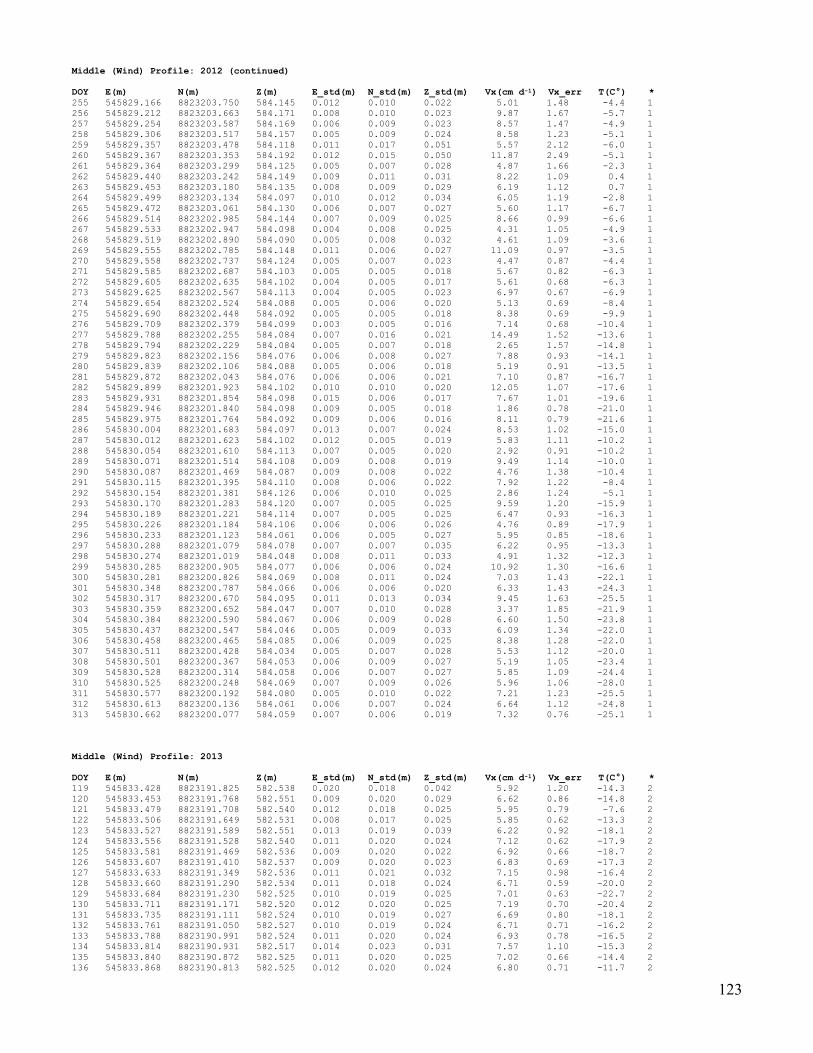
123
Middle (Wind) Profile: 2012 (continued)
DOY E(m) N(m) Z(m) E_std(m) N_std(m) Z_std(m) Vx(cm d-1) Vx_err T(C°) *
255 545829.166 8823203.750 584.145 0.012 0.010 0.022 5.01 1.48 -4.4 1
256 545829.212 8823203.663 584.171 0.008 0.010 0.023 9.87 1.67 -5.7 1
257 545829.254 8823203.587 584.169 0.006 0.009 0.023 8.57 1.47 -4.9 1
258 545829.306 8823203.517 584.157 0.005 0.009 0.024 8.58 1.23 -5.1 1
259 545829.357 8823203.478 584.118 0.011 0.017 0.051 5.57 2.12 -6.0 1
260 545829.367 8823203.353 584.192 0.012 0.015 0.050 11.87 2.49 -5.1 1
261 545829.364 8823203.299 584.125 0.005 0.007 0.028 4.87 1.66 -2.3 1
262 545829.440 8823203.242 584.149 0.009 0.011 0.031 8.22 1.09 0.4 1
263 545829.453 8823203.180 584.135 0.008 0.009 0.029 6.19 1.12 0.7 1
264 545829.499 8823203.134 584.097 0.010 0.012 0.034 6.05 1.19 -2.8 1
265 545829.472 8823203.061 584.130 0.006 0.007 0.027 5.60 1.17 -6.7 1
266 545829.514 8823202.985 584.144 0.007 0.009 0.025 8.66 0.99 -6.6 1
267 545829.533 8823202.947 584.098 0.004 0.008 0.025 4.31 1.05 -4.9 1
268 545829.519 8823202.890 584.090 0.005 0.008 0.032 4.61 1.09 -3.6 1
269 545829.555 8823202.785 584.148 0.011 0.006 0.027 11.09 0.97 -3.5 1
270 545829.558 8823202.737 584.124 0.005 0.007 0.023 4.47 0.87 -4.4 1
271 545829.585 8823202.687 584.103 0.005 0.005 0.018 5.67 0.82 -6.3 1
272 545829.605 8823202.635 584.102 0.004 0.005 0.017 5.61 0.68 -6.3 1
273 545829.625 8823202.567 584.113 0.004 0.005 0.023 6.97 0.67 -6.9 1
274 545829.654 8823202.524 584.088 0.005 0.006 0.020 5.13 0.69 -8.4 1
275 545829.690 8823202.448 584.092 0.005 0.005 0.018 8.38 0.69 -9.9 1
276 545829.709 8823202.379 584.099 0.003 0.005 0.016 7.14 0.68 -10.4 1
277 545829.788 8823202.255 584.084 0.007 0.016 0.021 14.49 1.52 -13.6 1
278 545829.794 8823202.229 584.084 0.005 0.007 0.018 2.65 1.57 -14.8 1
279 545829.823 8823202.156 584.076 0.006 0.008 0.027 7.88 0.93 -14.1 1
280 545829.839 8823202.106 584.088 0.005 0.006 0.018 5.19 0.91 -13.5 1
281 545829.872 8823202.043 584.076 0.006 0.006 0.021 7.10 0.87 -16.7 1
282 545829.899 8823201.923 584.102 0.010 0.010 0.020 12.05 1.07 -17.6 1
283 545829.931 8823201.854 584.098 0.015 0.006 0.017 7.67 1.01 -19.6 1
284 545829.946 8823201.840 584.098 0.009 0.005 0.018 1.86 0.78 -21.0 1
285 545829.975 8823201.764 584.092 0.009 0.006 0.016 8.11 0.79 -21.6 1
286 545830.004 8823201.683 584.097 0.013 0.007 0.024 8.53 1.02 -15.0 1
287 545830.012 8823201.623 584.102 0.012 0.005 0.019 5.83 1.11 -10.2 1
288 545830.054 8823201.610 584.113 0.007 0.005 0.020 2.92 0.91 -10.2 1
289 545830.071 8823201.514 584.108 0.009 0.008 0.019 9.49 1.14 -10.0 1
290 545830.087 8823201.469 584.087 0.009 0.008 0.022 4.76 1.38 -10.4 1
291 545830.115 8823201.395 584.110 0.008 0.006 0.022 7.92 1.22 -8.4 1
292 545830.154 8823201.381 584.126 0.006 0.010 0.025 2.86 1.24 -5.1 1
293 545830.170 8823201.283 584.120 0.007 0.005 0.025 9.59 1.20 -15.9 1
294 545830.189 8823201.221 584.114 0.007 0.005 0.025 6.47 0.93 -16.3 1
295 545830.226 8823201.184 584.106 0.006 0.006 0.026 4.76 0.89 -17.9 1
296 545830.233 8823201.123 584.061 0.006 0.005 0.027 5.95 0.85 -18.6 1
297 545830.288 8823201.079 584.078 0.007 0.007 0.035 6.22 0.95 -13.3 1
298 545830.274 8823201.019 584.048 0.008 0.011 0.033 4.91 1.32 -12.3 1
299 545830.285 8823200.905 584.077 0.006 0.006 0.024 10.92 1.30 -16.6 1
300 545830.281 8823200.826 584.069 0.008 0.011 0.024 7.03 1.43 -22.1 1
301 545830.348 8823200.787 584.066 0.006 0.006 0.020 6.33 1.43 -24.3 1
302 545830.317 8823200.670 584.095 0.011 0.013 0.034 9.45 1.63 -25.5 1
303 545830.359 8823200.652 584.047 0.007 0.010 0.028 3.37 1.85 -21.9 1
304 545830.384 8823200.590 584.067 0.006 0.009 0.028 6.60 1.50 -23.8 1
305 545830.437 8823200.547 584.046 0.005 0.009 0.033 6.09 1.34 -22.0 1
306 545830.458 8823200.465 584.085 0.006 0.009 0.025 8.38 1.28 -22.0 1
307 545830.511 8823200.428 584.034 0.005 0.007 0.028 5.53 1.12 -20.0 1
308 545830.501 8823200.367 584.053 0.006 0.009 0.027 5.19 1.05 -23.4 1
309 545830.528 8823200.314 584.058 0.006 0.007 0.027 5.85 1.09 -24.4 1
310 545830.525 8823200.248 584.069 0.007 0.009 0.026 5.96 1.06 -28.0 1
311 545830.577 8823200.192 584.080 0.005 0.010 0.022 7.21 1.23 -25.5 1
312 545830.613 8823200.136 584.061 0.006 0.007 0.024 6.64 1.12 -24.8 1
313 545830.662 8823200.077 584.059 0.007 0.006 0.019 7.32 0.76 -25.1 1
Middle (Wind) Profile: 2013
DOY E(m) N(m) Z(m) E_std(m) N_std(m) Z_std(m) Vx(cm d-1) Vx_err T(C°) *
119 545833.428 8823191.825 582.538 0.020 0.018 0.042 5.92 1.20 -14.3 2
120 545833.453 8823191.768 582.551 0.009 0.020 0.029 6.62 0.86 -14.8 2
121 545833.479 8823191.708 582.540 0.012 0.018 0.025 5.95 0.79 -7.6 2
122 545833.506 8823191.649 582.531 0.008 0.017 0.025 5.85 0.62 -13.3 2
123 545833.527 8823191.589 582.551 0.013 0.019 0.039 6.22 0.92 -18.1 2
124 545833.556 8823191.528 582.540 0.011 0.020 0.024 7.12 0.62 -17.9 2
125 545833.581 8823191.469 582.536 0.009 0.020 0.022 6.92 0.66 -18.7 2
126 545833.607 8823191.410 582.537 0.009 0.020 0.023 6.83 0.69 -17.3 2
127 545833.633 8823191.349 582.536 0.011 0.021 0.032 7.15 0.98 -16.4 2
128 545833.660 8823191.290 582.534 0.011 0.018 0.024 6.71 0.59 -20.0 2
129 545833.684 8823191.230 582.525 0.010 0.019 0.025 7.01 0.63 -22.7 2
130 545833.711 8823191.171 582.520 0.012 0.020 0.025 7.19 0.70 -20.4 2
131 545833.735 8823191.111 582.524 0.010 0.019 0.027 6.69 0.80 -18.1 2
132 545833.761 8823191.050 582.527 0.010 0.019 0.024 6.71 0.71 -16.2 2
133 545833.788 8823190.991 582.524 0.011 0.020 0.024 6.93 0.78 -16.5 2
134 545833.814 8823190.931 582.517 0.014 0.023 0.031 7.57 1.10 -15.3 2
135 545833.840 8823190.872 582.525 0.011 0.020 0.025 7.02 0.66 -14.4 2
136 545833.868 8823190.813 582.525 0.012 0.020 0.024 6.80 0.71 -11.7 2

124
Middle (Wind) Profile: 2013 (continued)
DOY E(m) N(m) Z(m) E_std(m) N_std(m) Z_std(m) Vx(cm d-1) Vx_err T(C°) *
137 545833.893 8823190.754 582.528 0.011 0.020 0.025 6.66 0.77 -7.5 2
138 545833.916 8823190.695 582.518 0.010 0.018 0.024 6.22 0.78 -6.3 2
139 545833.942 8823190.636 582.526 0.013 0.020 0.035 6.23 1.23 -7.8 2
140 545833.968 8823190.573 582.526 0.010 0.021 0.022 7.26 0.74 -9.9 2
141 545833.992 8823190.513 582.527 0.011 0.021 0.022 7.20 0.69 -9.9 2
142 545834.020 8823190.454 582.524 0.010 0.018 0.022 6.12 0.72 -8.2 2
143 545834.044 8823190.393 582.525 0.012 0.021 0.021 7.53 0.70 -8.9 2
144 545834.074 8823190.334 582.525 0.013 0.020 0.025 7.36 0.69 -9.0 2
145 545834.097 8823190.275 582.522 0.011 0.018 0.022 6.48 0.66 -5.2 2
146 545834.122 8823190.215 582.521 0.011 0.019 0.022 6.82 0.70 -4.4 2
147 545834.149 8823190.155 582.526 0.011 0.018 0.024 6.64 0.69 -1.8 2
148 545834.173 8823190.090 582.517 0.015 0.024 0.029 7.55 1.46 -3.0 2
149 545834.199 8823190.034 582.516 0.012 0.020 0.021 7.00 0.76 -5.1 2
150 545834.225 8823189.975 582.511 0.011 0.020 0.022 7.04 0.76 -6.4 2
151 545834.251 8823189.913 582.512 0.013 0.020 0.023 7.27 0.76 -6.9 2
152 545834.276 8823189.855 582.514 0.012 0.021 0.023 7.72 0.63 -5.0 2
153 545834.300 8823189.794 582.511 0.012 0.024 0.025 8.39 0.71 -6.6 2
154 545834.328 8823189.735 582.516 0.011 0.022 0.030 7.83 0.65 -7.9 2
155 545834.350 8823189.676 582.498 0.014 0.023 0.033 8.28 0.75 -8.8 2
156 545834.378 8823189.617 582.508 0.012 0.022 0.031 7.69 0.72 -10.2 2
157 545834.404 8823189.560 582.516 0.014 0.022 0.030 7.48 1.03 -5.9 2
158 545834.434 8823189.497 582.488 0.016 0.024 0.028 8.07 1.15 0.1 2
159 545834.453 8823189.437 582.492 0.020 0.025 0.033 9.89 0.88 -2.6 2
160 545834.486 8823189.380 582.487 0.019 0.023 0.041 6.83 1.20 -2.8 2
161 545834.508 8823189.314 582.498 0.013 0.024 0.026 8.62 0.76 -1.1 2
162 545834.538 8823189.254 582.502 0.012 0.022 0.028 7.83 0.81 -2.1 2
163 545834.564 8823189.197 582.498 0.011 0.021 0.027 7.03 0.97 1.7 2
164 545834.584 8823189.133 582.497 0.041 0.034 0.052 8.34 2.97 -0.2 2
165 545834.613 8823189.074 582.507 0.013 0.024 0.030 8.30 0.71 1.4 2
166 545834.638 8823189.021 582.496 0.011 0.018 0.037 6.09 0.76 -0.2 2
167 545834.665 8823188.956 582.510 0.012 0.020 0.029 7.35 0.68 -1.7 2
168 545834.688 8823188.897 582.460 0.011 0.024 0.038 8.12 0.74 -2.8 2
169 545834.722 8823188.838 582.476 0.013 0.021 0.034 7.36 0.90 -0.9 2
170 545834.745 8823188.773 582.490 0.016 0.023 0.030 8.47 1.05 -0.5 2
171 545834.767 8823188.715 582.492 0.012 0.024 0.032 8.28 0.80 -1.2 2
172 545834.793 8823188.656 582.496 0.012 0.022 0.027 8.07 0.78 -0.5 2
173 545834.821 8823188.595 582.492 0.012 0.020 0.026 7.39 0.72 -0.5 2
174 545834.847 8823188.536 582.494 0.012 0.020 0.025 7.42 0.76 -0.8 2
175 545834.873 8823188.476 582.513 0.013 0.022 0.047 7.81 0.79 -2.5 2
176 545834.899 8823188.417 582.489 0.013 0.020 0.034 7.43 0.70 -3.4 2
177 545834.923 8823188.355 582.489 0.019 0.021 0.031 6.76 1.01 -5.2 2
178 545834.956 8823188.297 582.495 0.015 0.019 0.028 6.96 0.81 -1.4 2
179 545834.976 8823188.235 582.490 0.013 0.023 0.027 8.08 0.81 1.6 2
180 545835.001 8823188.175 582.501 0.013 0.022 0.032 7.89 0.72 -0.0 2
181 545835.029 8823188.114 582.489 0.011 0.025 0.043 8.42 0.76 -0.7 2
182 545835.056 8823188.050 582.474 0.013 0.019 0.032 6.20 0.88 -2.8 2
183 545835.083 8823187.991 582.487 0.010 0.020 0.025 6.90 0.66 1.9 2
184 545835.110 8823187.931 582.476 0.012 0.022 0.026 7.75 0.78 3.2 2
185 545835.139 8823187.871 582.471 0.014 0.022 0.028 7.92 0.84 2.5 2
186 545835.162 8823187.808 582.468 0.013 0.022 0.030 8.01 0.85 1.1 2
187 545835.190 8823187.748 582.466 0.014 0.019 0.029 7.11 0.80 1.7 2
188 545835.217 8823187.686 582.467 0.013 0.021 0.028 7.57 0.75 3.5 2
189 545835.243 8823187.621 582.470 0.013 0.021 0.026 7.54 0.81 3.0 2
190 545835.271 8823187.556 582.467 0.014 0.020 0.030 7.64 0.78 3.2 2
191 545835.298 8823187.493 582.458 0.014 0.021 0.032 7.52 0.75 3.6 2
192 545835.330 8823187.424 582.467 0.014 0.020 0.032 7.20 0.85 4.5 2
193 545835.359 8823187.362 582.469 0.016 0.021 0.030 7.56 0.88 3.4 2
194 545835.386 8823187.290 582.459 0.014 0.027 0.033 9.55 1.00 4.8 2
195 545835.418 8823187.226 582.450 0.011 0.022 0.028 7.60 0.83 4.1 2
196 545835.447 8823187.156 582.454 0.011 0.020 0.027 6.96 0.68 5.3 2
197 545835.481 8823187.080 582.450 0.012 0.024 0.025 8.36 0.85 5.4 2
198 545835.513 8823187.000 582.446 0.012 0.026 0.027 8.97 0.94 5.8 2
199 545835.552 8823186.930 582.441 0.015 0.023 0.029 8.06 1.02 4.6 2
200 545835.585 8823186.856 582.426 0.017 0.033 0.056 7.23 2.67 6.7 2
201 545835.618 8823186.767 582.437 0.015 0.023 0.028 8.64 0.84 4.4 2
202 545835.654 8823186.689 582.433 0.014 0.024 0.025 8.85 0.74 5.1 2
203 545835.691 8823186.598 582.437 0.016 0.028 0.025 10.73 0.72 5.5 2
204 545835.753 8823186.439 582.470 0.030 0.071 0.037 26.04 1.34 4.6 2
205 545835.826 8823186.244 582.516 0.023 0.051 0.034 18.75 1.00 3.1 2
206 545835.888 8823186.123 582.512 0.018 0.024 0.031 9.11 0.94 -0.3 2
207 545835.926 8823186.039 582.475 0.014 0.023 0.024 8.23 0.97 -3.0 2
208 545835.962 8823185.961 582.472 0.011 0.023 0.022 8.37 0.57 -2.3 2
209 545835.999 8823185.887 582.458 0.016 0.022 0.024 8.06 0.90 -1.0 2
210 545836.031 8823185.812 582.462 0.013 0.020 0.023 7.71 0.60 -1.7 2
211 545836.065 8823185.735 582.461 0.011 0.021 0.024 7.52 0.64 -0.8 2
212 545836.099 8823185.661 582.456 0.019 0.018 0.026 6.73 1.23 -1.2 2
213 545836.136 8823185.575 582.458 0.039 0.026 0.045 6.08 2.43 1.2 2
214 545836.163 8823185.506 582.458 0.012 0.022 0.026 8.12 0.64 1.9 2
215 545836.195 8823185.431 582.458 0.014 0.020 0.025 7.63 0.64 1.4 2
216 545836.233 8823185.351 582.460 0.015 0.020 0.027 7.57 0.64 1.4 2
217 545836.279 8823185.247 582.466 0.027 0.054 0.031 19.80 1.55 3.0 2
218 545836.403 8823184.929 582.563 0.037 0.076 0.040 28.00 2.10 3.1 2
219 545836.494 8823184.727 582.576 0.029 0.043 0.031 17.10 1.22 2.9 2

125
Middle (Wind) Profile: 2013 (continued)
DOY E(m) N(m) Z(m) E_std(m) N_std(m) Z_std(m) Vx(cm d-1) Vx_err T(C°) *
220 545836.558 8823184.614 582.540 0.024 0.023 0.030 9.37 1.04 2.0 2
221 545836.607 8823184.529 582.500 0.017 0.021 0.036 7.60 0.89 2.1 2
222 545836.670 8823184.374 582.540 0.038 0.093 0.063 32.57 3.15 3.2 2
223 545836.790 8823184.099 582.564 0.028 0.029 0.043 11.93 1.26 1.4 2
224 545836.840 8823184.017 582.513 0.026 0.022 0.044 6.30 1.51 -0.3 2
225 545836.885 8823183.933 582.477 0.016 0.024 0.031 9.37 0.74 -1.9 2
226 545836.922 8823183.855 582.466 0.013 0.023 0.030 8.16 0.77 -2.9 2
227 545836.960 8823183.775 582.454 0.014 0.020 0.030 7.49 0.73 -3.8 2
228 545836.991 8823183.699 582.425 0.015 0.022 0.024 8.00 0.91 -5.4 2
229 545837.023 8823183.623 582.452 0.014 0.022 0.022 8.15 0.79 -6.0 2
230 545837.057 8823183.550 582.434 0.014 0.022 0.030 8.01 0.75 -5.5 2
231 545837.087 8823183.474 582.440 0.013 0.020 0.025 7.33 0.66 -7.5 2
232 545837.118 8823183.401 582.435 0.012 0.018 0.026 6.85 0.61 -8.3 2
233 545837.147 8823183.327 582.435 0.013 0.022 0.024 7.95 0.69 -7.0 2
234 545837.187 8823183.254 582.446 0.031 0.023 0.090 4.97 2.38 -7.5 2
235 545837.211 8823183.190 582.426 0.014 0.019 0.023 6.70 0.79 -8.8 2
236 545837.237 8823183.113 582.441 0.013 0.024 0.035 7.78 0.93 -0.1 2
237 545837.274 8823183.045 582.441 0.016 0.021 0.023 8.12 0.86 0.9 2
238 545837.308 8823182.973 582.439 0.017 0.024 0.026 9.03 0.87 -1.6 2
239 545837.332 8823182.906 582.428 0.012 0.024 0.025 8.26 0.83 -3.2 2
240 545837.358 8823182.834 582.437 0.021 0.023 0.029 6.80 1.29 -3.1 2
241 545837.392 8823182.768 582.427 0.014 0.021 0.027 7.39 0.89 -3.2 2
242 545837.423 8823182.701 582.429 0.011 0.022 0.024 7.53 0.72 -4.5 2
243 545837.453 8823182.632 582.430 0.013 0.020 0.026 7.13 0.75 -6.8 2
244 545837.478 8823182.567 582.423 0.012 0.020 0.025 6.71 0.77 -5.7 2
245 545837.511 8823182.491 582.429 0.015 0.021 0.024 7.14 0.94 -4.2 2
246 545837.542 8823182.424 582.426 0.016 0.020 0.029 7.09 0.87 -4.4 2
247 545837.572 8823182.356 582.410 0.019 0.020 0.030 6.92 1.27 -4.9 2
248 545837.598 8823182.295 582.420 0.015 0.017 0.028 5.43 0.91 -8.0 2
249 545837.629 8823182.221 582.420 0.016 0.018 0.025 6.80 0.69 -10.4 2
250 545837.659 8823182.155 582.410 0.013 0.018 0.026 6.58 0.72 -4.8 2
251 545837.689 8823182.085 582.411 0.010 0.021 0.027 6.75 0.82 -1.7 2
252 545837.720 8823182.019 582.415 0.010 0.019 0.023 6.65 0.71 -2.9 2
253 545837.747 8823181.950 582.412 0.012 0.024 0.025 7.58 0.96 -3.9 2
254 545837.783 8823181.885 582.413 0.021 0.018 0.033 6.30 1.18 -3.4 2
255 545837.806 8823181.813 582.411 0.010 0.025 0.026 8.02 0.80 -5.9 2
256 545837.837 8823181.744 582.411 0.009 0.021 0.025 7.36 0.67 -7.2 2
257 545837.866 8823181.676 582.408 0.009 0.023 0.025 7.81 0.74 -7.9 2
258 545837.895 8823181.612 582.403 0.012 0.019 0.030 6.32 0.71 -9.2 2
259 545837.923 8823181.542 582.402 0.010 0.024 0.024 8.31 0.69 -5.9 2
260 545837.949 8823181.472 582.405 0.018 0.027 0.043 7.56 1.58 -5.7 2
261 545837.984 8823181.406 582.408 0.011 0.022 0.023 7.83 0.67 -9.2 2
262 545838.012 8823181.338 582.407 0.011 0.023 0.024 8.15 0.74 -10.2 2
263 545838.043 8823181.270 582.408 0.011 0.021 0.022 7.56 0.63 -9.3 2
264 545838.072 8823181.203 582.410 0.012 0.023 0.023 8.17 0.72 -11.2 2
265 545838.102 8823181.137 582.410 0.011 0.023 0.024 8.11 0.71 -10.1 2
266 545838.136 8823181.070 582.401 0.014 0.021 0.031 7.80 0.71 -11.1 2
267 545838.164 8823181.004 582.398 0.010 0.018 0.027 5.98 0.83 -13.9 2
268 545838.192 8823180.925 582.404 0.024 0.023 0.049 6.68 1.72 -12.1 2
269 545838.219 8823180.866 582.402 0.010 0.021 0.028 7.39 0.64 -10.7 2
270 545838.249 8823180.801 582.403 0.009 0.019 0.026 6.50 0.67 -7.2 2
Middle (Wind) Profile: 2014
DOY E(m) N(m) Z(m) E_std(m) N_std(m) Z_std(m) Vx(cm d-1) Vx_err T(C°) *
116 545844.342 8823166.853 582.220 0.011 0.021 0.025 7.23 0.77 -11.3 2
117 545844.369 8823166.788 582.222 0.012 0.019 0.024 6.68 0.77 -12.4 2
118 545844.397 8823166.725 582.227 0.012 0.019 0.024 6.84 0.66 -13.1 2
119 545844.422 8823166.658 582.222 0.011 0.020 0.024 7.00 0.76 -11.4 2
120 545844.459 8823166.599 582.210 0.032 0.021 0.057 5.52 1.42 -12.6 2
121 545844.480 8823166.530 582.220 0.012 0.021 0.022 7.13 0.88 -13.2 2
122 545844.512 8823166.466 582.215 0.014 0.020 0.025 6.93 1.06 -9.3 2
123 545844.536 8823166.402 582.222 0.011 0.020 0.026 6.92 0.72 -13.5 2
124 545844.559 8823166.366 582.233 0.006 0.006 0.028 1.98 0.54 -13.1 2
125 545844.585 8823166.274 582.202 0.036 0.036 0.038 2.94 3.13 -13.0 2
126 545844.618 8823166.206 582.232 0.020 0.019 0.049 4.68 1.31 -9.5 2
127 545844.647 8823166.147 582.230 0.012 0.020 0.027 6.74 0.85 -9.9 2
128 545844.671 8823166.104 582.238 0.007 0.007 0.024 2.78 0.71 -8.9 2
191 545845.046 8823163.708 581.346 0.304 0.486 0.136 - - 4.5 2
192 545845.024 8823163.722 581.333 0.018 0.033 0.030 12.04 0.73 3.0 2
193 545845.074 8823163.616 581.325 0.017 0.032 0.030 11.70 0.72 3.2 2
194 545845.124 8823163.521 581.302 0.019 0.022 0.029 8.13 0.69 2.6 2
195 545845.170 8823163.429 581.291 0.024 0.030 0.026 11.52 0.72 5.6 2
196 545845.230 8823163.282 581.291 0.023 0.046 0.027 16.67 1.00 6.9 2
197 545845.286 8823163.151 581.303 0.023 0.024 0.059 7.49 1.52 5.0 2
198 545845.334 8823163.049 581.292 0.015 0.029 0.028 10.62 0.71 2.4 2
199 545845.377 8823162.959 581.282 0.013 0.029 0.030 10.08 0.82 4.0 2
200 545845.424 8823162.856 581.284 0.014 0.027 0.031 9.67 0.79 4.8 2
201 545845.471 8823162.755 581.282 0.017 0.034 0.026 12.28 0.88 4.9 2
202 545845.519 8823162.649 581.280 0.017 0.028 0.031 10.25 0.73 4.5 2

126
Middle (Wind) Profile: 2015
DOY E(m) N(m) Z(m) E_std(m) N_std(m) Z_std(m) Vx(cm d-1) Vx_err T(C°) *
114 545854.158 8823143.151 581.099 0.011 0.020 0.019 7.25 0.64 -10.4 2
115 545854.185 8823143.085 581.113 0.013 0.023 0.027 8.04 0.91 -10.0 2
116 545854.217 8823143.015 581.149 0.012 0.020 0.024 7.20 0.69 -10.3 2
117 545854.245 8823142.951 581.152 0.013 0.021 0.025 7.57 0.76 -13.7 2
118 545854.274 8823142.888 581.149 0.013 0.020 0.024 7.46 0.73 -15.2 2
119 545854.303 8823142.822 581.149 0.012 0.022 0.024 7.82 0.72 -16.5 2
120 545854.331 8823142.759 581.147 0.012 0.022 0.027 7.60 0.87 -16.1 2
121 545854.357 8823142.696 581.149 0.012 0.021 0.027 7.04 0.94 -15.4 2
122 545854.388 8823142.630 581.146 0.013 0.021 0.025 7.77 0.74 -14.5 2
123 545854.409 8823142.561 581.140 0.020 0.030 0.040 8.87 1.17 -14.7 2
124 545854.443 8823142.502 581.144 0.013 0.023 0.025 8.37 0.82 -12.9 2
125 545854.473 8823142.439 581.144 0.012 0.022 0.024 7.66 0.79 -14.4 2
126 545854.501 8823142.373 581.140 0.012 0.021 0.030 7.66 0.84 -16.5 2
127 545854.531 8823142.310 581.145 0.014 0.020 0.024 7.70 0.80 -17.1 2
128 545854.559 8823142.245 581.143 0.012 0.021 0.024 7.61 0.79 -17.5 2
129 545854.589 8823142.180 581.142 0.014 0.021 0.023 7.56 0.75 -15.8 2
130 545854.617 8823142.115 581.152 0.013 0.023 0.029 8.29 0.82 -12.5 2
131 545854.635 8823142.052 581.142 0.031 0.032 0.053 10.64 2.41 -15.0 2
132 545854.677 8823141.991 581.145 0.026 0.029 0.046 8.09 1.95 -15.1 2
133 545854.703 8823141.925 581.137 0.011 0.024 0.024 8.27 0.78 -16.4 2
134 545854.730 8823141.858 581.126 0.012 0.022 0.027 7.92 0.70 -15.1 2
135 545854.759 8823141.794 581.130 0.014 0.025 0.032 9.04 0.81 -12.4 2
136 545854.788 8823141.731 581.147 0.013 0.022 0.026 8.27 0.78 -9.4 2
137 545854.814 8823141.666 581.144 0.011 0.021 0.026 7.40 0.78 -8.8 2
138 545854.848 8823141.603 581.139 0.015 0.021 0.030 7.37 1.12 -7.2 2
139 545854.875 8823141.538 581.135 0.012 0.023 0.027 8.17 0.72 -8.6 2
140 545854.902 8823141.474 581.148 0.013 0.021 0.030 7.79 0.77 -7.6 2
141 545854.930 8823141.409 581.132 0.013 0.023 0.026 8.51 0.74 -8.8 2
142 545854.960 8823141.347 581.120 0.012 0.021 0.031 7.35 0.79 -12.9 2
143 545854.987 8823141.279 581.126 0.013 0.022 0.027 8.11 0.66 -13.9 2
144 545855.017 8823141.213 581.127 0.012 0.022 0.026 7.88 0.72 -6.4 2
145 545855.042 8823141.150 581.126 0.011 0.023 0.026 8.11 0.80 -6.7 2
146 545855.074 8823141.086 581.130 0.014 0.024 0.027 8.46 0.94 -3.0 2
147 545855.105 8823141.021 581.129 0.013 0.023 0.026 8.15 0.89 -2.8 2
148 545855.131 8823140.958 581.129 0.016 0.023 0.030 8.18 1.17 -3.5 2
149 545855.157 8823140.892 581.133 0.012 0.023 0.026 8.09 0.85 -2.3 2
150 545855.187 8823140.828 581.130 0.011 0.023 0.026 8.28 0.65 -1.3 2
151 545855.217 8823140.763 581.133 0.013 0.023 0.025 8.49 0.66 0.3 2
152 545855.244 8823140.699 581.124 0.012 0.021 0.025 7.82 0.67 0.8 2
153 545855.271 8823140.631 581.127 0.013 0.021 0.025 8.02 0.64 -0.9 2
154 545855.302 8823140.568 581.128 0.014 0.022 0.024 8.27 0.65 1.8 2
155 545855.333 8823140.503 581.125 0.014 0.021 0.025 7.91 0.69 0.8 2
156 545855.362 8823140.438 581.129 0.016 0.022 0.024 8.58 0.72 -0.7 2
157 545855.392 8823140.370 581.130 0.014 0.021 0.023 7.62 0.78 -2.4 2
158 545855.420 8823140.307 581.131 0.014 0.019 0.029 6.21 1.10 -3.8 2
159 545855.451 8823140.232 581.137 0.015 0.024 0.032 8.93 0.72 -0.7 2
160 545855.482 8823140.170 581.132 0.014 0.021 0.025 7.25 1.03 1.6 2
161 545855.512 8823140.099 581.129 0.010 0.021 0.025 7.62 0.68 1.2 2
162 545855.541 8823140.034 581.125 0.012 0.021 0.026 7.69 0.75 0.6 2
163 545855.570 8823139.965 581.127 0.014 0.023 0.025 8.50 0.83 1.1 2
164 545855.601 8823139.897 581.121 0.014 0.023 0.027 8.34 0.80 2.6 2
165 545855.632 8823139.830 581.117 0.014 0.023 0.029 8.62 0.88 4.0 2
166 545855.671 8823139.751 581.118 0.016 0.025 0.027 9.29 0.92 3.2 2
167 545855.705 8823139.667 581.124 0.018 0.027 0.028 10.30 0.75 2.5 2
168 545855.746 8823139.576 581.123 0.017 0.030 0.027 10.62 0.83 4.1 2
169 545855.795 8823139.465 581.128 0.019 0.038 0.028 13.97 1.18 2.7 2
170 545855.837 8823139.345 581.127 0.022 0.036 0.030 13.79 0.94 2.1 2
171 545855.891 8823139.229 581.121 0.021 0.037 0.024 14.29 0.66 2.5 2
172 545855.949 8823139.093 581.155 0.023 0.040 0.029 15.46 0.90 3.0 2
173 545855.994 8823138.980 581.185 0.022 0.033 0.030 12.54 1.09 3.1 2
174 545856.043 8823138.874 581.180 0.019 0.032 0.028 12.04 0.91 2.5 2
175 545856.091 8823138.774 581.179 0.018 0.030 0.030 11.58 0.75 3.2 2
176 545856.137 8823138.677 581.172 0.016 0.027 0.026 10.22 0.68 1.2 2
177 545856.179 8823138.586 581.176 0.017 0.029 0.024 10.84 0.86 3.0 2
178 545856.231 8823138.484 581.180 0.022 0.030 0.028 11.88 1.05 3.4 2
179 545856.301 8823138.339 581.176 0.049 0.039 0.075 11.32 3.36 5.6 2
180 545856.356 8823138.197 581.180 0.024 0.048 0.026 18.13 0.80 3.7 2
181 545856.422 8823138.032 581.230 0.026 0.040 0.027 15.82 0.94 2.5 2
182 545856.478 8823137.904 581.216 0.026 0.043 0.032 15.50 1.77 4.9 2
183 545856.553 8823137.750 581.239 0.028 0.048 0.025 18.72 0.93 3.5 2
184 545856.622 8823137.591 581.250 0.034 0.049 0.038 19.21 1.37 3.5 2
185 545856.696 8823137.423 581.263 0.034 0.065 0.028 24.70 1.52 5.4 2
186 545856.805 8823137.169 581.293 0.032 0.034 0.047 14.24 1.35 4.9 2
187 545856.883 8823137.056 581.247 0.022 0.042 0.030 15.30 1.19 6.7 2
188 545856.955 8823136.898 581.260 0.028 0.061 0.027 22.75 1.08 8.1 2
189 545857.029 8823136.737 581.268 0.025 0.044 0.027 16.65 1.16 8.1 2
190 545857.099 8823136.608 581.261 0.022 0.032 0.031 12.75 0.93 9.3 2
191 545857.158 8823136.501 581.224 0.020 0.036 0.027 13.90 0.73 7.7 2
192 545857.218 8823136.372 581.225 0.024 0.055 0.026 19.51 1.70 7.4 2
193 545857.296 8823136.208 581.221 0.020 0.036 0.024 13.62 0.80 8.1 2
194 545857.356 8823136.096 581.213 0.029 0.041 0.025 15.97 1.39 7.2 2
195 545857.400 8823136.003 581.190 0.024 0.045 0.059 15.79 1.80 7.2 2
196 545857.449 8823135.890 581.183 0.021 0.033 0.024 12.88 0.77 6.0 2
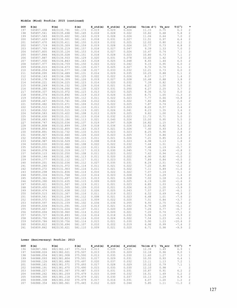
127
Middle (Wind) Profile: 2015 (continued)
DOY E(m) N(m) Z(m) E_std(m) N_std(m) Z_std(m) Vx(cm d-1) Vx_err T(C°) *
197 545857.498 8823135.791 581.173 0.019 0.029 0.024 11.15 0.75 6.3 2
198 545857.541 8823135.698 581.165 0.018 0.028 0.022 10.82 0.68 5.8 2
199 545857.583 8823135.602 581.163 0.019 0.028 0.024 11.06 0.64 7.0 2
200 545857.629 8823135.501 581.161 0.018 0.031 0.027 11.51 0.97 6.4 2
201 545857.670 8823135.411 581.155 0.019 0.032 0.025 12.02 0.80 6.2 2
202 545857.719 8823135.309 581.159 0.019 0.028 0.024 10.77 0.73 6.8 2
203 545857.765 8823135.219 581.157 0.018 0.027 0.047 9.39 1.33 7.0 2
204 545857.805 8823135.124 581.153 0.016 0.027 0.024 10.47 0.74 7.1 2
205 545857.846 8823135.028 581.151 0.018 0.028 0.023 10.80 0.73 7.1 2
206 545857.887 8823134.933 581.129 0.020 0.031 0.078 10.60 1.42 7.0 2
207 545857.930 8823134.843 581.143 0.018 0.025 0.048 8.65 1.44 6.5 2
208 545857.977 8823134.759 581.150 0.023 0.022 0.042 9.15 0.95 6.0 2
209 545858.015 8823134.673 581.135 0.017 0.025 0.027 9.72 0.76 5.1 2
210 545858.054 8823134.577 581.138 0.017 0.033 0.032 12.21 0.73 6.0 2
211 545858.095 8823134.489 581.131 0.014 0.029 0.035 10.25 0.88 5.1 2
212 545858.143 8823134.398 581.125 0.022 0.022 0.026 8.57 1.17 1.4 2
213 545858.178 8823134.309 581.126 0.019 0.027 0.028 10.48 0.88 3.8 2
214 545858.221 8823134.225 581.123 0.014 0.020 0.032 7.39 0.82 4.5 2
215 545858.249 8823134.152 581.129 0.016 0.021 0.041 6.27 1.50 5.0 2
216 545858.285 8823134.066 581.135 0.023 0.031 0.050 6.27 2.25 3.7 2
217 545858.337 8823133.972 581.115 0.013 0.023 0.025 8.36 0.72 0.0 2
218 545858.374 8823133.892 581.119 0.013 0.026 0.025 8.71 1.05 -1.3 2
219 545858.411 8823133.815 581.112 0.011 0.022 0.023 7.77 0.66 -0.8 2
220 545858.447 8823133.741 581.104 0.012 0.022 0.022 7.82 0.86 2.6 2
221 545858.482 8823133.671 581.104 0.012 0.022 0.025 7.87 0.74 2.1 2
222 545858.512 8823133.592 581.110 0.011 0.023 0.023 8.22 0.57 2.4 2
223 545858.552 8823133.515 581.119 0.021 0.026 0.041 8.23 1.35 3.6 2
224 545858.583 8823133.422 581.108 0.013 0.029 0.025 9.82 1.00 5.6 2
225 545858.630 8823133.311 581.115 0.016 0.032 0.023 11.73 0.71 5.0 2
226 545858.683 8823133.186 581.113 0.021 0.040 0.024 15.00 0.95 5.5 2
227 545858.747 8823133.036 581.137 0.019 0.047 0.028 16.82 1.15 5.1 2
228 545858.808 8823132.899 581.159 0.018 0.034 0.024 12.82 0.82 4.3 2
229 545858.854 8823132.805 581.143 0.013 0.021 0.026 7.40 0.93 3.4 2
230 545858.891 8823132.732 581.133 0.015 0.023 0.023 8.25 0.90 2.8 2
231 545858.927 8823132.660 581.126 0.010 0.023 0.025 7.63 0.86 1.8 2
232 545858.963 8823132.586 581.115 0.011 0.021 0.024 7.21 0.85 2.6 2
233 545858.987 8823132.529 581.111 0.008 0.018 0.023 4.98 1.13 1.8 2
234 545859.020 8823132.462 581.108 0.022 0.022 0.032 7.44 1.51 1.1 2
235 545859.051 8823132.388 581.110 0.011 0.024 0.025 7.48 1.19 -0.7 2
236 545859.078 8823132.319 581.117 0.013 0.030 0.045 7.76 1.69 -0.8 2
237 545859.115 8823132.250 581.108 0.011 0.023 0.022 7.62 0.94 -1.2 2
238 545859.146 8823132.182 581.113 0.011 0.020 0.022 6.90 0.82 -0.0 2
239 545859.177 8823132.112 581.117 0.011 0.023 0.021 7.89 0.84 -0.5 2
240 545859.201 8823132.036 581.112 0.027 0.035 0.031 8.24 2.51 -0.8 2
241 545859.240 8823131.972 581.114 0.011 0.021 0.022 7.22 0.80 -2.2 2
242 545859.272 8823131.903 581.116 0.011 0.021 0.022 7.11 0.89 -1.6 2
243 545859.298 8823131.836 581.114 0.010 0.022 0.022 7.07 1.14 0.1 2
244 545859.334 8823131.768 581.110 0.014 0.023 0.028 7.63 1.29 1.4 2
245 545859.361 8823131.697 581.115 0.013 0.021 0.028 7.02 1.18 -1.4 2
246 545859.390 8823131.635 581.115 0.009 0.020 0.025 6.19 1.00 -1.6 2
247 545859.421 8823131.567 581.119 0.011 0.021 0.023 6.85 1.03 -2.6 2
248 545859.450 8823131.505 581.109 0.010 0.021 0.026 6.33 1.20 -3.9 2
249 545859.474 8823131.438 581.112 0.026 0.025 0.043 7.57 2.07 -6.1 2
250 545859.515 8823131.367 581.116 0.011 0.019 0.023 6.52 0.69 -4.9 2
251 545859.541 8823131.299 581.112 0.008 0.021 0.023 6.48 1.01 -7.6 2
252 545859.572 8823131.226 581.115 0.009 0.022 0.020 7.51 0.84 -3.7 2
253 545859.597 8823131.159 581.102 0.034 0.036 0.055 9.93 2.75 -2.6 2
254 545859.634 8823131.091 581.110 0.013 0.021 0.032 6.78 1.09 -6.1 2
255 545859.667 8823131.024 581.107 0.011 0.020 0.020 7.26 0.77 -6.7 2
256 545859.694 8823130.960 581.114 0.012 0.020 0.021 7.20 0.74 -7.1 2
257 545859.727 8823130.893 581.116 0.014 0.018 0.032 5.94 1.19 -5.9 2
258 545859.750 8823130.823 581.114 0.010 0.024 0.022 7.54 1.23 -4.1 2
259 545859.786 8823130.756 581.114 0.015 0.021 0.030 5.90 1.23 -10.4 2
260 545859.812 8823130.694 581.107 0.010 0.022 0.019 6.96 0.99 -7.4 2
261 545859.842 8823130.621 581.110 0.009 0.021 0.020 6.71 0.98 -9.9 2
Lower (Anniversary) Profile: 2013
DOY E(m) N(m) Z(m) E_std(m) N_std(m) Z_std(m) Vx(cm d-1) Vx_err T(C°) *
196 546987.986 8821382.147 375.514 0.013 0.039 0.035 12.39 1.49 6.9 1
197 546988.026 8821382.021 375.507 0.013 0.035 0.029 12.18 0.96 8.0 1
198 546988.054 8821381.908 375.500 0.013 0.035 0.030 11.60 1.27 7.3 1
199 546988.093 8821381.804 375.501 0.017 0.029 0.031 10.55 0.93 6.4 1
200 546988.126 8821381.686 375.497 0.020 0.037 0.032 13.11 1.13 7.2 1
201 546988.161 8821381.571 375.493 0.017 0.028 0.029 10.12 0.79 7.1 1
202 546988.191 8821381.470 375.490 0.015 0.035 0.030 12.10 0.98 - 2
203 546988.227 8821381.367 375.487 0.015 0.031 0.031 10.87 0.91 6.2 2
204 546988.262 8821381.259 375.479 0.015 0.049 0.032 16.51 1.69 5.2 2
205 546988.300 8821381.118 375.479 0.021 0.030 0.037 10.13 1.29 4.9 2
206 546988.338 8821381.032 375.479 0.017 0.016 0.031 4.07 1.20 1.2 2
207 546988.354 8821380.961 375.445 0.012 0.020 0.044 5.85 1.11 -1.3 2

128
Lower (Anniversary) Profile: 2013 (continued)
DOY E(m) N(m) Z(m) E_std(m) N_std(m) Z_std(m) Vx(cm d-1) Vx_err T(C°) *
208 546988.384 8821380.899 375.435 0.009 0.018 0.029 4.77 0.96 -1.1 2
209 546988.407 8821380.829 375.426 0.014 0.028 0.026 9.58 0.97 -1.0 2
210 546988.429 8821380.747 375.420 0.010 0.015 0.027 4.25 0.81 -1.0 2
211 546988.447 8821380.693 375.413 0.011 0.016 0.025 4.37 0.89 0.2 2
212 546988.464 8821380.642 375.408 0.010 0.013 0.027 4.05 0.66 0.5 2
213 546988.485 8821380.589 375.406 0.011 0.017 0.027 5.47 0.71 1.3 2
214 546988.511 8821380.528 375.410 0.014 0.020 0.029 6.64 0.90 1.7 2
215 546988.530 8821380.459 375.399 0.011 0.021 0.026 6.94 0.76 0.7 2
216 546988.555 8821380.381 375.399 0.011 0.020 0.028 6.59 0.69 2.0 2
217 546988.604 8821380.235 375.416 0.025 0.083 0.030 29.40 1.21 4.0 2
218 546988.673 8821379.934 375.436 0.031 0.068 0.033 24.74 1.50 3.8 2
219 546988.744 8821379.738 375.421 0.022 0.037 0.034 14.00 0.98 3.2 2
220 546988.791 8821379.638 375.392 0.021 0.017 0.029 6.47 0.85 1.8 2
221 546988.827 8821379.570 375.353 0.023 0.024 0.059 4.63 2.13 2.5 2
222 546988.868 8821379.452 375.392 0.023 0.063 0.039 21.80 1.59 4.2 2
223 546988.944 8821379.201 375.391 0.026 0.032 0.041 11.68 1.61 1.6 2
224 546988.984 8821379.130 375.352 0.020 0.014 0.040 4.12 1.10 0.0 2
225 546989.014 8821379.067 375.318 0.011 0.020 0.032 7.11 0.66 -0.6 2
226 546989.033 8821379.006 375.318 0.009 0.018 0.029 5.40 0.77 -2.2 2
227 546989.057 8821378.944 375.313 0.008 0.016 0.034 5.26 0.66 -2.8 2
228 546989.074 8821378.896 375.291 0.009 0.017 0.029 5.40 0.75 -4.1 2
229 546989.093 8821378.840 375.303 0.009 0.016 0.024 5.44 0.65 -4.9 2
230 546989.112 8821378.790 375.292 0.009 0.016 0.031 5.04 0.77 -4.0 2
231 546989.124 8821378.735 375.290 0.010 0.016 0.025 4.82 0.85 -6.4 2
232 546989.151 8821378.681 375.274 0.018 0.016 0.036 6.34 0.76 -6.8 2
233 546989.161 8821378.633 375.282 0.009 0.020 0.026 6.63 0.80 -5.7 2
234 546989.176 8821378.583 375.276 0.024 0.021 0.051 6.09 1.67 -6.3 2
235 546989.198 8821378.536 375.278 0.008 0.016 0.024 4.63 0.77 -8.0 2
236 546989.210 8821378.483 375.280 0.009 0.020 0.036 5.22 1.22 0.6 2
237 546989.236 8821378.435 375.278 0.012 0.017 0.025 4.59 1.21 2.2 2
238 546989.255 8821378.386 375.275 0.012 0.018 0.029 6.46 0.87 -2.6 2
239 546989.265 8821378.340 375.264 0.007 0.019 0.028 5.94 0.79 -4.6 2
240 546989.283 8821378.286 375.271 0.011 0.024 0.031 6.03 1.58 -3.4 2
241 546989.300 8821378.247 375.260 0.007 0.017 0.030 5.02 0.82 -4.4 2
242 546989.317 8821378.200 375.262 0.008 0.017 0.028 5.15 0.76 -4.9 2
243 546989.335 8821378.154 375.262 0.008 0.015 0.026 4.93 0.72 -6.1 2
244 546989.347 8821378.109 375.255 0.009 0.017 0.028 4.83 0.79 -5.0 2
245 546989.366 8821378.058 375.257 0.009 0.016 0.025 4.64 0.79 -2.9 2
246 546989.383 8821378.012 375.260 0.009 0.016 0.028 4.73 0.78 -2.3 2
247 546989.400 8821377.969 375.249 0.007 0.016 0.026 4.93 0.69 -3.3 2
248 546989.414 8821377.923 375.250 0.008 0.016 0.027 5.08 0.82 -6.7 2
249 546989.434 8821377.879 375.247 0.008 0.018 0.029 4.99 0.92 -8.3 2
250 546989.446 8821377.831 375.243 0.007 0.015 0.029 4.11 0.97 -5.4 2
251 546989.464 8821377.785 375.243 0.008 0.018 0.029 4.68 0.98 0.2 2
252 546989.480 8821377.740 375.243 0.007 0.018 0.026 4.80 1.03 -0.8 2
253 546989.488 8821377.696 375.242 0.028 0.034 0.073 6.24 2.93 -2.1 2
254 546989.512 8821377.655 375.230 0.017 0.018 0.034 3.97 1.22 -1.4 2
255 546989.529 8821377.602 375.235 0.007 0.018 0.029 4.78 0.87 -3.3 2
256 546989.547 8821377.556 375.236 0.008 0.016 0.028 4.67 0.87 -5.0 2
257 546989.562 8821377.511 375.231 0.007 0.018 0.027 5.47 0.77 -5.8 2
258 546989.578 8821377.467 375.232 0.006 0.017 0.026 5.27 0.79 -7.8 2
259 546989.594 8821377.421 375.228 0.007 0.018 0.026 5.66 0.79 -7.4 2
260 546989.611 8821377.376 375.233 0.007 0.019 0.029 5.57 0.88 -5.5 2
261 546989.628 8821377.331 375.231 0.007 0.019 0.025 5.66 0.84 -8.3 2
262 546989.642 8821377.285 375.229 0.008 0.019 0.026 5.92 0.85 -9.1 2
263 546989.660 8821377.241 375.229 0.007 0.017 0.024 5.18 0.77 -7.9 2
264 546989.676 8821377.196 375.231 0.009 0.019 0.025 6.15 0.83 -11.9 2
265 546989.693 8821377.153 375.230 0.009 0.019 0.026 5.98 0.78 -9.4 2
266 546989.710 8821377.108 375.225 0.009 0.018 0.026 5.55 0.80 -11.7 2
267 546989.726 8821377.063 375.220 0.008 0.017 0.027 4.97 0.74 -13.4 2
268 546989.742 8821377.016 375.222 0.008 0.019 0.025 6.07 0.72 -11.3 2
269 546989.757 8821376.973 375.220 0.010 0.017 0.028 5.43 0.75 -10.9 2
270 546989.774 8821376.930 375.218 0.010 0.016 0.027 4.56 0.73 -5.9 2
271 546989.799 8821376.885 375.220 0.017 0.020 0.026 6.08 1.28 -6.4 2
272 546989.792 8821376.841 375.221 0.032 0.030 0.042 9.59 1.59 -8.5 2
Lower (Anniversary) Profile: 2014
DOY E(m) N(m) Z(m) E_std(m) N_std(m) Z_std(m) Vx(cm d-1) Vx_err T(C°) *
113 546992.977 8821368.015 374.949 0.010 0.015 0.031 5.10 0.72 -15.4 2
114 546992.993 8821367.975 374.954 0.010 0.016 0.027 5.30 0.73 -14.9 2
115 546993.005 8821367.929 374.956 0.013 0.019 0.029 6.41 0.82 -10.8 2
116 546993.021 8821367.892 374.954 0.008 0.017 0.025 5.74 0.65 -9.5 2
117 546993.036 8821367.851 374.951 0.008 0.014 0.023 4.81 0.61 -11.9 2
118 546993.052 8821367.811 374.952 0.010 0.014 0.026 4.75 0.61 -12.7 2
119 546993.065 8821367.768 374.947 0.009 0.014 0.024 4.58 0.65 -9.2 2
120 546993.087 8821367.731 374.933 0.029 0.016 0.054 3.68 1.13 -11.5 2
121 546993.093 8821367.685 374.945 0.009 0.015 0.023 5.11 0.62 -11.3 2
122 546993.111 8821367.644 374.943 0.011 0.015 0.026 5.23 0.74 -10.2 2
123 546993.124 8821367.603 374.942 0.009 0.013 0.026 4.34 0.58 -14.9 2
124 546993.128 8821367.557 374.948 0.036 0.022 0.034 5.11 0.97 -14.6 2
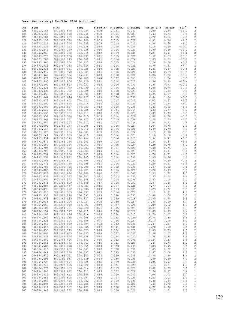
129
Lower (Anniversary) Profile: 2014 (continued)
DOY E(m) N(m) Z(m) E_std(m) N_std(m) Z_std(m) Vx(cm d-1) Vx_err T(C°) *
125 546993.165 8821367.528 374.934 0.028 0.021 0.043 1.99 2.24 -11.0 2
126 546993.168 8821367.478 374.948 0.008 0.014 0.027 4.43 0.74 -8.9 2
127 546993.184 8821367.439 374.946 0.008 0.015 0.025 4.72 0.66 -9.8 2
128 546993.196 8821367.398 374.949 0.009 0.015 0.022 4.41 0.76 -9.0 2
129 546993.213 8821367.356 374.935 0.009 0.015 0.022 4.98 0.64 -8.0 2
130 546993.229 8821367.313 374.938 0.010 0.015 0.021 5.18 0.59 -10.2 2
131 546993.245 8821367.269 374.936 0.010 0.016 0.020 5.39 0.60 -12.1 2
132 546993.262 8821367.230 374.945 0.012 0.019 0.035 6.24 0.91 -11.6 2
133 546993.274 8821367.186 374.937 0.011 0.015 0.021 5.52 0.63 -13.7 2
134 546993.289 8821367.145 374.942 0.011 0.016 0.024 5.89 0.63 -10.8 2
135 546993.303 8821367.104 374.923 0.010 0.015 0.024 5.26 0.66 -6.8 2
136 546993.319 8821367.062 374.928 0.011 0.014 0.021 4.88 0.61 -7.7 2
137 546993.333 8821367.021 374.928 0.010 0.015 0.020 5.41 0.67 -10.5 2
138 546993.347 8821366.978 374.934 0.011 0.015 0.020 5.43 0.59 -10.8 2
139 546993.362 8821366.934 374.931 0.013 0.018 0.021 6.26 0.70 -10.3 2
140 546993.371 8821366.898 374.940 0.024 0.022 0.053 7.19 1.24 -8.9 2
141 546993.395 8821366.856 374.929 0.011 0.014 0.022 4.36 0.93 -10.6 2
142 546993.404 8821366.813 374.932 0.013 0.016 0.030 5.38 0.93 -10.0 2
143 546993.421 8821366.770 374.930 0.009 0.016 0.022 5.48 0.70 -10.0 2
144 546993.435 8821366.732 374.929 0.010 0.018 0.027 4.66 1.34 -5.1 2
145 546993.453 8821366.684 374.932 0.011 0.018 0.027 6.35 0.77 -2.8 2
146 546993.462 8821366.646 374.927 0.013 0.020 0.030 6.44 1.06 -3.0 2
147 546993.479 8821366.602 374.921 0.010 0.017 0.025 6.02 0.67 -6.2 2
148 546993.490 8821366.554 374.914 0.014 0.022 0.030 5.78 1.24 -3.1 2
149 546993.509 8821366.517 374.920 0.012 0.015 0.025 5.43 0.62 -3.5 2
150 546993.519 8821366.465 374.925 0.022 0.034 0.064 7.83 1.77 -5.0 2
151 546993.538 8821366.434 374.917 0.010 0.015 0.023 4.89 0.73 -6.1 2
152 546993.551 8821366.394 374.915 0.009 0.014 0.022 4.82 0.70 -5.5 2
153 546993.562 8821366.351 374.922 0.013 0.019 0.034 5.60 1.29 -1.0 2
154 546993.584 8821366.307 374.913 0.011 0.017 0.026 5.44 0.92 1.8 2
155 546993.599 8821366.267 374.908 0.010 0.015 0.027 5.04 0.75 1.9 2
156 546993.616 8821366.224 374.910 0.010 0.016 0.026 5.49 0.79 2.0 2
157 546993.629 8821366.183 374.907 0.009 0.015 0.024 5.19 0.70 -0.1 2
158 546993.644 8821366.139 374.910 0.010 0.014 0.023 5.10 0.68 -5.2 2
159 546993.659 8821366.098 374.904 0.011 0.016 0.023 5.34 0.72 -5.5 2
160 546993.675 8821366.054 374.903 0.010 0.015 0.022 5.24 0.67 -4.5 2
161 546993.689 8821366.014 374.903 0.011 0.015 0.024 5.29 0.70 -3.6 2
162 546993.705 8821365.972 374.903 0.012 0.014 0.026 4.90 0.76 -3.3 2
163 546993.720 8821365.928 374.903 0.013 0.014 0.027 4.79 0.81 -3.4 2
164 546993.732 8821365.886 374.903 0.013 0.014 0.027 4.76 0.71 -1.5 2
165 546993.751 8821365.842 374.905 0.010 0.014 0.030 3.85 0.96 1.3 2
166 546993.763 8821365.801 374.896 0.012 0.013 0.024 4.42 0.69 -0.3 2
167 546993.778 8821365.758 374.898 0.011 0.016 0.023 5.20 0.81 -1.9 2
168 546993.788 8821365.715 374.900 0.013 0.012 0.030 3.47 0.92 -0.6 2
169 546993.805 8821365.668 374.901 0.010 0.016 0.028 5.20 0.89 3.8 2
170 546993.826 8821365.624 374.900 0.020 0.021 0.040 5.53 1.72 4.7 2
171 546993.839 8821365.587 374.881 0.011 0.013 0.035 3.93 0.98 3.4 2
172 546993.854 8821365.552 374.888 0.020 0.015 0.036 2.43 1.18 6.1 2
173 546993.876 8821365.509 374.889 0.017 0.018 0.053 1.87 1.45 4.1 2
174 546993.886 8821365.457 374.881 0.015 0.017 0.031 4.77 1.14 3.2 2
175 546993.898 8821365.412 374.883 0.013 0.013 0.027 4.29 0.72 2.9 2
176 546993.910 8821365.365 374.897 0.009 0.016 0.028 5.11 0.71 4.1 2
177 546993.938 8821365.298 374.897 0.019 0.034 0.035 12.48 1.08 5.2 2
178 546993.973 8821365.165 374.927 0.016 0.039 0.028 13.85 0.78 6.9 2
179 546994.018 8821365.004 374.927 0.020 0.050 0.027 17.98 0.99 5.7 2
180 546994.063 8821364.840 374.922 0.019 0.037 0.025 13.89 0.62 4.8 2
181 546994.106 8821364.701 374.928 0.021 0.035 0.027 12.97 0.81 0.7 2
182 546994.152 8821364.577 374.912 0.016 0.028 0.028 10.09 0.83 2.4 2
183 546994.207 8821364.436 374.916 0.023 0.054 0.027 19.79 1.07 5.1 2
184 546994.262 8821364.280 374.908 0.020 0.053 0.028 18.78 1.35 5.9 2
185 546994.321 8821364.106 374.905 0.021 0.046 0.027 16.13 1.18 6.2 2
186 546994.369 8821363.969 374.894 0.022 0.033 0.039 11.47 1.27 3.9 2
187 546994.416 8821363.854 374.885 0.017 0.041 0.031 13.78 1.50 8.4 2
188 546994.455 8821363.745 374.873 0.014 0.024 0.029 8.49 0.79 7.0 2
189 546994.487 8821363.653 374.850 0.014 0.032 0.031 10.56 1.07 4.2 2
190 546994.522 8821363.564 374.838 0.014 0.034 0.027 11.94 0.84 4.8 2
191 546994.552 8821363.456 374.851 0.010 0.042 0.031 13.24 1.23 5.9 2
192 546994.561 8821363.353 374.862 0.015 0.021 0.029 7.44 0.74 4.2 2
193 546994.586 8821363.278 374.855 0.013 0.023 0.034 7.83 0.95 3.1 2
194 546994.615 8821363.202 374.847 0.017 0.020 0.031 7.85 0.82 2.9 2
195 546994.642 8821363.130 374.837 0.021 0.025 0.030 9.37 1.08 7.8 2
196 546994.675 8821363.041 374.840 0.023 0.029 0.029 10.80 1.30 8.6 2
197 546994.698 8821362.961 374.839 0.018 0.020 0.031 7.59 0.99 7.0 2
198 546994.724 8821362.894 374.825 0.015 0.019 0.031 6.85 0.97 2.8 2
199 546994.745 8821362.835 374.820 0.013 0.021 0.029 7.15 0.81 4.5 2
200 546994.776 8821362.753 374.814 0.011 0.019 0.029 6.02 0.93 6.6 1
201 546994.804 8821362.682 374.811 0.013 0.022 0.026 7.56 0.97 6.6 1
202 546994.829 8821362.612 374.808 0.015 0.020 0.033 7.06 1.02 5.7 1
203 546994.851 8821362.548 374.797 0.015 0.017 0.029 5.53 1.03 4.3 1
204 546994.868 8821362.486 374.782 0.022 0.019 0.036 5.40 1.44 -0.5 1
205 546994.894 8821362.419 374.780 0.013 0.021 0.028 7.44 0.72 1.3 1
206 546994.917 8821362.357 374.771 0.014 0.020 0.027 6.72 0.80 5.3 1
207 546994.943 8821362.292 374.768 0.013 0.020 0.029 6.27 1.01 3.3 1
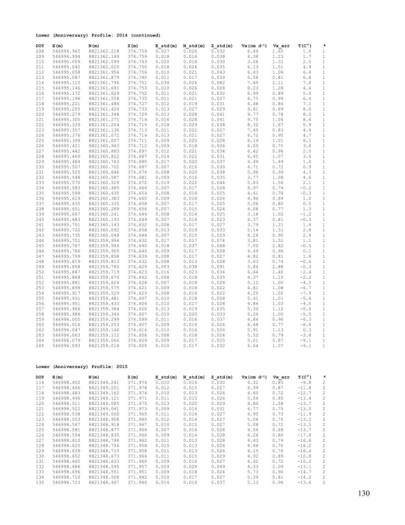
130
Lower (Anniversary) Profile: 2014 (continued)
DOY E(m) N(m) Z(m) E_std(m) N_std(m) Z_std(m) Vx(cm d-1) Vx_err T(C°) *
208 546994.965 8821362.218 374.759 0.027 0.026 0.032 6.49 1.65 1.6 1
209 546994.994 8821362.149 374.759 0.018 0.016 0.038 4.38 1.23 1.7 1
210 546995.009 8821362.099 374.743 0.020 0.018 0.030 3.08 1.31 2.5 1
211 546995.040 8821362.025 374.750 0.018 0.024 0.035 6.13 1.51 4.9 1
212 546995.058 8821361.954 374.756 0.010 0.021 0.043 6.43 1.06 6.4 1
213 546995.087 8821361.879 374.740 0.011 0.017 0.030 5.58 0.81 6.8 1
214 546995.110 8821361.796 374.751 0.034 0.026 0.082 7.60 2.11 7.6 1
215 546995.146 8821361.691 374.753 0.010 0.026 0.028 8.23 1.28 4.4 1
216 546995.172 8821361.629 374.752 0.011 0.021 0.032 6.99 0.89 5.0 1
217 546995.196 8821361.558 374.735 0.011 0.021 0.027 6.75 0.99 6.4 1
218 546995.221 8821361.486 374.727 0.012 0.019 0.031 6.48 0.86 7.1 1
219 546995.255 8821361.424 374.733 0.013 0.027 0.029 9.61 0.89 8.0 1
220 546995.279 8821361.348 374.729 0.013 0.028 0.041 9.77 0.78 8.5 1
221 546995.305 8821361.271 374.714 0.016 0.028 0.041 9.75 1.04 8.6 1
222 546995.339 8821361.204 374.715 0.018 0.029 0.038 8.32 1.67 5.9 1
223 546995.357 8821361.136 374.713 0.011 0.022 0.027 7.45 0.83 4.4 1
224 546995.376 8821361.072 374.714 0.013 0.021 0.027 6.72 0.95 4.7 1
225 546995.399 8821361.007 374.711 0.009 0.020 0.028 6.19 1.01 6.1 1
226 546995.421 8821360.943 374.712 0.009 0.018 0.026 6.00 0.75 3.6 1
227 546995.442 8821360.883 374.697 0.012 0.021 0.034 6.42 0.96 2.0 1
228 546995.469 8821360.822 374.687 0.014 0.022 0.031 6.45 1.07 3.4 1
229 546995.484 8821360.763 374.685 0.017 0.020 0.037 4.49 1.49 1.4 1
230 546995.507 8821360.702 374.687 0.007 0.016 0.030 4.71 0.72 0.9 1
231 546995.525 8821360.646 374.676 0.008 0.020 0.038 5.96 0.99 4.3 1
232 546995.548 8821360.587 374.681 0.009 0.016 0.035 3.77 1.08 4.6 1
233 546995.570 8821360.529 374.672 0.019 0.022 0.044 5.83 1.56 2.1 1
234 546995.583 8821360.485 374.664 0.007 0.017 0.028 4.97 0.74 -0.2 1
235 546995.599 8821360.435 374.654 0.008 0.016 0.025 4.41 0.78 -0.3 1
236 546995.619 8821360.383 374.660 0.009 0.016 0.026 4.96 0.84 1.0 1
237 546995.635 8821360.335 374.658 0.007 0.017 0.025 5.06 0.80 0.5 1
238 546995.651 8821360.289 374.656 0.007 0.015 0.024 4.08 0.77 1.3 1
239 546995.667 8821360.241 374.644 0.008 0.014 0.025 3.18 1.02 -1.2 1
240 546995.683 8821360.193 374.649 0.007 0.016 0.023 4.37 0.81 -0.3 1
241 546995.701 8821360.143 374.652 0.008 0.017 0.027 3.79 1.21 1.4 1
242 546995.722 8821360.092 374.658 0.013 0.019 0.033 5.14 1.31 2.8 1
243 546995.735 8821360.048 374.646 0.007 0.015 0.029 4.24 0.90 2.4 1
244 546995.751 8821359.994 374.632 0.017 0.017 0.074 3.81 1.51 1.1 1
245 546995.767 8821359.944 374.640 0.018 0.037 0.068 7.00 2.82 -0.5 1
246 546995.786 8821359.905 374.640 0.009 0.017 0.028 4.49 0.96 0.1 1
247 546995.799 8821359.858 374.639 0.008 0.017 0.027 4.82 0.81 1.6 1
248 546995.819 8821359.813 374.632 0.008 0.013 0.028 3.63 0.74 -0.6 1
249 546995.858 8821359.765 374.625 0.053 0.038 0.091 3.84 2.88 -0.3 1
250 546995.847 8821359.719 374.623 0.016 0.023 0.034 6.44 1.40 -2.4 1
251 546995.868 8821359.670 374.642 0.008 0.018 0.035 4.37 1.15 -2.2 1
252 546995.881 8821359.624 374.626 0.007 0.018 0.028 5.12 1.00 -4.5 1
253 546995.899 8821359.575 374.621 0.009 0.018 0.022 4.81 1.08 -6.7 1
254 546995.917 8821359.529 374.623 0.008 0.016 0.022 4.25 1.02 -7.9 1
255 546995.931 8821359.481 374.607 0.010 0.018 0.028 5.41 1.01 -5.6 1
256 546995.951 8821359.433 374.604 0.010 0.017 0.028 4.84 1.03 -4.5 1
257 546995.966 8821359.384 374.620 0.013 0.019 0.035 5.30 1.12 -5.6 1
258 546995.986 8821359.344 374.607 0.010 0.020 0.033 5.26 1.00 -5.5 1
259 546996.005 8821359.299 374.599 0.011 0.016 0.037 4.84 0.96 -6.3 1
260 546996.016 8821359.253 374.607 0.009 0.016 0.024 4.48 0.77 -6.4 1
262 546996.047 8821359.146 374.616 0.010 0.016 0.026 5.91 1.13 0.3 1
263 546996.063 8821359.112 374.606 0.008 0.018 0.024 5.52 0.79 -3.8 1
264 546996.079 8821359.066 374.609 0.009 0.017 0.025 5.01 0.87 -9.1 1
265 546996.093 8821359.018 374.605 0.010 0.017 0.032 4.64 1.07 -9.1 1
Lower (Anniversary) Profile: 2015
DOY E(m) N(m) Z(m) E_std(m) N_std(m) Z_std(m) Vx(cm d-1) Vx_err T(C°) *
116 546998.452 8821349.241 371.974 0.010 0.014 0.030 4.32 0.85 -9.8 2
117 546998.466 8821349.201 371.978 0.012 0.015 0.027 4.99 0.87 -11.8 2
118 546998.483 8821349.162 371.974 0.010 0.013 0.026 4.60 0.72 -12.7 2
119 546998.496 8821349.121 371.971 0.011 0.015 0.026 5.04 0.85 -13.4 2
120 546998.511 8821349.085 371.975 0.013 0.020 0.029 4.80 1.58 -13.7 2
121 546998.522 8821349.041 371.973 0.009 0.014 0.031 4.77 0.75 -13.0 2
122 546998.538 8821349.000 371.965 0.011 0.014 0.027 4.95 0.73 -11.9 2
123 546998.553 8821348.958 371.965 0.012 0.014 0.027 5.04 0.75 -13.2 2
124 546998.567 8821348.918 371.967 0.010 0.015 0.027 5.08 0.72 -13.5 2
125 546998.581 8821348.877 371.966 0.007 0.014 0.026 4.54 0.69 -13.7 2
126 546998.594 8821348.835 371.960 0.009 0.014 0.028 4.26 0.80 -17.8 2
127 546998.610 8821348.796 371.962 0.011 0.013 0.028 4.43 0.74 -16.6 2
128 546998.625 8821348.756 371.958 0.010 0.013 0.026 4.48 0.70 -16.2 2
129 546998.639 8821348.715 371.958 0.011 0.013 0.026 4.15 0.76 -16.4 2
130 546998.652 8821348.673 371.966 0.011 0.015 0.029 4.92 0.89 -12.8 2
131 546998.665 8821348.633 371.960 0.009 0.014 0.027 4.42 0.72 -15.2 2
132 546998.686 8821348.595 371.957 0.029 0.024 0.049 4.33 2.09 -13.1 2
133 546998.696 8821348.551 371.951 0.009 0.018 0.024 5.73 0.90 -14.7 2
134 546998.710 8821348.508 371.942 0.010 0.017 0.027 5.39 0.81 -14.2 2
135 546998.723 8821348.467 371.940 0.014 0.016 0.037 5.13 0.96 -13.6 2

131
Lower (Anniversary) Profile: 2015 (continued)
DOY E(m) N(m) Z(m) E_std(m) N_std(m) Z_std(m) Vx(cm d-1) Vx_err T(C°) *
136 546998.740 8821348.427 371.957 0.009 0.014 0.027 4.77 0.73 -11.1 2
137 546998.752 8821348.387 371.957 0.009 0.014 0.030 4.18 0.81 -8.9 2
138 546998.769 8821348.347 371.947 0.010 0.013 0.031 4.29 0.75 -6.9 2
139 546998.786 8821348.305 371.941 0.010 0.014 0.028 4.78 0.77 -8.1 2
140 546998.797 8821348.265 371.952 0.010 0.015 0.030 4.72 0.74 -7.7 2
141 546998.812 8821348.223 371.934 0.010 0.015 0.026 5.16 0.78 -7.4 2
142 546998.829 8821348.181 371.924 0.011 0.018 0.042 5.67 0.98 -13.4 2
143 546998.840 8821348.139 371.931 0.010 0.017 0.029 5.54 0.83 -12.3 2
144 546998.856 8821348.096 371.929 0.010 0.017 0.027 5.44 0.81 -5.4 2
145 546998.870 8821348.056 371.922 0.008 0.018 0.031 4.93 1.05 -5.5 2
146 546998.884 8821348.016 371.927 0.012 0.017 0.027 5.61 0.95 -2.5 2
147 546998.900 8821347.973 371.922 0.010 0.016 0.029 5.23 0.87 -2.3 2
148 546998.915 8821347.933 371.929 0.009 0.015 0.030 4.87 0.76 -4.2 2
149 546998.924 8821347.893 371.926 0.009 0.015 0.027 4.74 0.83 -3.0 2
150 546998.940 8821347.852 371.919 0.013 0.015 0.029 4.94 0.86 -1.4 2
151 546998.955 8821347.809 371.916 0.012 0.016 0.025 5.31 0.83 1.9 2
152 546998.969 8821347.768 371.916 0.012 0.016 0.028 5.48 0.79 2.3 2
153 546998.983 8821347.722 371.925 0.012 0.019 0.031 5.98 1.09 -1.1 2
154 546999.013 8821347.678 371.917 0.035 0.027 0.065 5.10 2.58 0.3 2
155 546999.014 8821347.643 371.917 0.011 0.014 0.027 4.90 0.72 -0.8 2
156 546999.028 8821347.601 371.915 0.011 0.014 0.026 4.96 0.69 -1.9 2
157 546999.043 8821347.561 371.919 0.010 0.013 0.023 4.27 0.65 -2.0 2
158 546999.055 8821347.520 371.916 0.010 0.013 0.029 3.14 0.89 -2.5 2
159 546999.074 8821347.472 371.916 0.011 0.015 0.030 4.92 0.90 0.0 2
160 546999.089 8821347.434 371.910 0.010 0.013 0.029 4.05 0.81 1.8 2
161 546999.103 8821347.389 371.904 0.008 0.013 0.028 4.10 0.71 0.7 2
162 546999.120 8821347.347 371.902 0.009 0.013 0.028 4.29 0.65 0.6 2
163 546999.135 8821347.303 371.900 0.010 0.014 0.026 4.96 0.70 0.7 2
164 546999.150 8821347.258 371.897 0.012 0.014 0.027 4.93 0.75 2.3 2
165 546999.168 8821347.214 371.899 0.015 0.016 0.030 5.79 0.91 4.7 2
166 546999.194 8821347.153 371.915 0.015 0.017 0.030 6.15 0.79 4.5 2
167 546999.214 8821347.094 371.916 0.014 0.021 0.029 7.61 0.69 3.6 2
168 546999.238 8821347.025 371.904 0.012 0.022 0.029 7.47 0.71 4.7 2
169 546999.274 8821346.911 371.905 0.020 0.038 0.036 13.46 1.18 2.1 2
170 546999.299 8821346.773 371.925 0.033 0.038 0.033 13.60 2.08 2.4 2
171 546999.337 8821346.674 371.909 0.016 0.027 0.038 9.51 1.11 2.9 2
172 546999.371 8821346.579 371.919 0.017 0.028 0.032 10.27 1.06 4.1 2
173 546999.397 8821346.489 371.920 0.014 0.027 0.032 9.94 0.81 4.9 2
174 546999.429 8821346.391 371.909 0.017 0.029 0.036 10.40 1.01 4.1 2
175 546999.460 8821346.302 371.915 0.013 0.025 0.034 9.22 0.71 4.7 2
176 546999.489 8821346.216 371.903 0.012 0.021 0.028 7.52 0.72 2.0 2
177 546999.515 8821346.145 371.897 0.012 0.022 0.027 7.68 0.85 4.6 2
178 546999.550 8821346.043 371.909 0.015 0.036 0.040 12.99 0.73 6.6 2
179 546999.593 8821345.893 371.912 0.021 0.051 0.032 18.47 1.14 7.3 2
180 546999.647 8821345.744 371.913 0.018 0.025 0.032 9.80 0.71 4.9 2
181 546999.685 8821345.640 371.895 0.016 0.043 0.026 15.57 0.84 4.1 2
182 546999.719 8821345.515 371.889 0.019 0.039 0.033 13.39 1.43 7.1 2
183 546999.770 8821345.400 371.886 0.028 0.020 0.035 7.27 1.38 6.0 2
184 546999.793 8821345.269 371.874 0.033 0.036 0.062 13.70 1.33 5.4 2
185 546999.856 8821345.128 371.892 0.026 0.060 0.032 21.62 1.47 7.2 2
186 546999.922 8821344.902 371.882 0.026 0.054 0.048 18.45 2.37 7.0 2
187 546999.973 8821344.790 371.864 0.014 0.031 0.056 10.66 1.14 8.9 2
188 547000.012 8821344.680 371.846 0.017 0.041 0.032 14.57 1.18 10.7 2
189 547000.048 8821344.570 371.839 0.013 0.030 0.026 10.55 0.98 10.7 2
190 547000.076 8821344.475 371.820 0.018 0.030 0.031 10.74 0.93 12.4 2
191 547000.110 8821344.394 371.798 0.012 0.026 0.027 9.19 0.67 9.7 2
192 547000.142 8821344.307 371.786 0.012 0.027 0.027 9.60 0.69 9.9 2
193 547000.173 8821344.217 371.777 0.013 0.024 0.025 8.68 0.75 11.4 2
194 547000.202 8821344.132 371.760 0.014 0.028 0.024 10.33 0.71 10.7 2
195 547000.223 8821344.051 371.745 0.012 0.026 0.028 9.06 0.71 9.2 2
196 547000.251 8821343.971 371.722 0.014 0.028 0.025 10.08 0.83 9.2 2
197 547000.277 8821343.873 371.712 0.011 0.034 0.028 11.70 0.92 7.2 2
198 547000.304 8821343.787 371.697 0.018 0.025 0.029 8.83 1.22 6.6 2
199 547000.319 8821343.714 371.689 0.018 0.024 0.031 8.28 0.97 7.3 2
200 547000.355 8821343.628 371.687 0.015 0.029 0.033 10.24 1.07 7.8 2
201 547000.380 8821343.548 371.657 0.020 0.027 0.047 9.16 1.02 6.8 2
202 547000.409 8821343.470 371.658 0.012 0.023 0.025 8.03 0.64 8.0 2
203 547000.437 8821343.386 371.637 0.011 0.025 0.026 8.78 0.67 10.3 2
204 547000.460 8821343.309 371.627 0.012 0.024 0.027 8.67 0.71 8.7 2
205 547000.485 8821343.231 371.616 0.013 0.024 0.025 8.66 0.69 8.7 2
206 547000.511 8821343.154 371.598 0.010 0.029 0.024 10.09 0.77 8.9 2
207 547000.537 8821343.074 371.584 0.010 0.026 0.025 8.94 0.85 8.2 2
208 547000.568 8821342.994 371.571 0.020 0.020 0.039 7.26 0.90 5.8 2
209 547000.590 8821342.920 371.555 0.011 0.023 0.028 7.92 0.74 6.0 2
210 547000.614 8821342.840 371.544 0.010 0.027 0.025 9.23 0.65 7.2 2
211 547000.639 8821342.754 371.525 0.011 0.026 0.026 9.25 0.77 6.0 2
212 547000.669 8821342.672 371.502 0.025 0.023 0.071 7.14 1.59 1.7 2
213 547000.692 8821342.602 371.504 0.013 0.025 0.024 8.98 0.75 4.8 2
214 547000.723 8821342.522 371.491 0.014 0.023 0.027 8.50 0.80 6.2 2
215 547000.744 8821342.452 371.484 0.014 0.020 0.029 6.59 0.90 6.2 2
216 547000.772 8821342.376 371.486 0.013 0.028 0.038 8.34 1.39 5.1 2
217 547000.794 8821342.300 371.456 0.008 0.021 0.026 7.21 0.71 0.6 2
218 547000.820 8821342.237 371.446 0.014 0.019 0.026 6.25 0.83 -0.6 2

132
Lower (Anniversary) Profile: 2015 (continued)
DOY E(m) N(m) Z(m) E_std(m) N_std(m) Z_std(m) Vx(cm d-1) Vx_err T(C°) *
219 547000.836 8821342.170 371.438 0.008 0.021 0.025 7.01 0.66 0.5 2
220 547000.858 8821342.114 371.433 0.011 0.020 0.030 6.68 0.84 1.8 2
221 547000.874 8821342.056 371.412 0.020 0.024 0.031 6.07 1.52 2.2 2
222 547000.905 8821341.987 371.423 0.009 0.021 0.025 6.73 0.92 1.4 2
223 547000.934 8821341.923 371.434 0.018 0.024 0.038 7.28 1.38 4.1 2
224 547000.955 8821341.844 371.423 0.011 0.030 0.035 9.49 1.26 6.2 2
225 547000.982 8821341.754 371.426 0.012 0.023 0.037 7.62 0.97 6.8 2
226 547001.008 8821341.670 371.411 0.012 0.030 0.024 10.54 1.03 6.3 2
227 547001.035 8821341.580 371.411 0.010 0.027 0.026 8.90 0.95 6.5 2
228 547001.068 8821341.511 371.411 0.009 0.026 0.024 8.58 0.95 5.8 2
229 547001.086 8821341.442 371.400 0.008 0.020 0.026 6.03 0.95 1.8 2
230 547001.114 8821341.384 371.402 0.009 0.018 0.026 5.08 1.01 1.2 2
231 547001.129 8821341.327 371.386 0.012 0.017 0.040 5.46 0.89 1.8 2
232 547001.152 8821341.269 371.381 0.009 0.018 0.025 5.64 0.89 3.3 2
233 547001.170 8821341.216 371.368 0.008 0.018 0.034 5.75 0.78 2.5 2
234 547001.195 8821341.160 371.370 0.027 0.022 0.042 6.69 1.47 1.5 2
235 547001.215 8821341.113 371.361 0.019 0.023 0.046 4.78 1.80 0.1 2
236 547001.229 8821341.053 371.365 0.011 0.019 0.025 5.77 0.90 0.1 2
237 547001.247 8821341.001 371.361 0.010 0.018 0.024 5.61 0.73 -0.5 2
238 547001.263 8821340.952 371.362 0.010 0.018 0.024 5.43 0.88 1.6 2
239 547001.281 8821340.903 371.363 0.009 0.018 0.023 5.70 0.77 0.8 2
240 547001.293 8821340.851 371.354 0.015 0.026 0.028 6.04 1.61 1.3 2
241 547001.316 8821340.806 371.354 0.007 0.017 0.025 5.37 0.86 -0.7 2
242 547001.325 8821340.757 371.351 0.017 0.024 0.025 5.20 1.70 -0.2 2
243 547001.347 8821340.710 371.346 0.007 0.016 0.025 4.65 0.89 0.4 2
244 547001.368 8821340.660 371.348 0.011 0.020 0.028 6.23 1.12 3.1 2
245 547001.381 8821340.614 371.346 0.010 0.018 0.025 5.70 0.88 0.1 2
246 547001.397 8821340.568 371.343 0.015 0.019 0.046 4.66 1.36 0.1 2
247 547001.415 8821340.521 371.342 0.009 0.015 0.024 4.69 0.81 -1.4 2
248 547001.427 8821340.484 371.332 0.010 0.015 0.030 4.25 0.89 -2.7 2
249 547001.447 8821340.438 371.330 0.011 0.012 0.027 2.54 1.04 -4.9 2
250 547001.464 8821340.388 371.340 0.017 0.023 0.035 6.60 1.21 -3.8 2
251 547001.480 8821340.337 371.333 0.009 0.018 0.021 5.51 0.80 -5.5 2
252 547001.499 8821340.294 371.331 0.011 0.023 0.026 6.47 1.08 -2.1 2
253 547001.504 8821340.244 371.322 0.031 0.028 0.047 6.88 1.82 -1.3 2
254 547001.530 8821340.195 371.330 0.010 0.016 0.024 5.13 0.80 -4.2 2
255 547001.545 8821340.152 371.318 0.008 0.019 0.023 5.28 1.04 -5.9 2
256 547001.560 8821340.106 371.315 0.010 0.015 0.047 4.18 1.07 -5.5 2
257 547001.574 8821340.063 371.329 0.017 0.018 0.039 5.70 1.04 -4.4 2
258 547001.592 8821340.016 371.318 0.009 0.015 0.021 5.27 0.64 -3.6 2
259 547001.600 8821339.970 371.314 0.014 0.017 0.032 4.71 0.89 -9.3 2
260 547001.622 8821339.927 371.306 0.009 0.018 0.022 5.01 0.91 -6.3 2
261 547001.636 8821339.878 371.312 0.008 0.015 0.022 3.85 0.94 -8.4 2
262 547001.655 8821339.846 371.309 0.009 0.016 0.033 -1.95 1.63 -9.1 2
263 547001.671 8821339.780 371.303 0.008 0.012 0.022 4.75 0.78 -10.0 2
264 547001.685 8821339.735 371.310 0.012 0.021 0.035 5.05 1.71 -11.4 2
265 547001.704 8821339.699 371.301 0.008 0.018 0.024 5.46 0.90 -10.5 2
266 547001.722 8821339.647 371.306 0.017 0.023 0.029 7.53 1.30 -8.4 2
267 547001.741 8821339.601 371.315 0.019 0.014 0.031 4.49 1.36 -9.9 2
Recommended