Antenna Report: Glaciers and Ice Sheets Mapping …research.bpcrc.osu.edu/rsl/gismo/documents/Gismo_Antenna_Report... · Antenna Report: Glaciers and Ice ... The Glaciers and Ice

Victor A. Jara

Antenna Report: Glaciers and Ice Sheets Mapping Orbiter

(GISMO) EECS 891 – Graduate Problems

Center for Remote Sensing of Ice Sheets

The University of Kansas

Aug.10, 2006

Center for Remote Sensing of Ice Sheets (CReSIS)

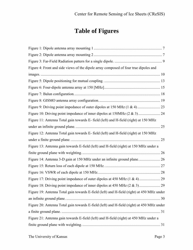
Table of Contents

1. Abstract ....................................................................................................................... 5

2. Introduction................................................................................................................. 6

3. Antenna Theory .......................................................................................................... 8

3.1. The single dipole................................................................................................. 8

3.2. Image theory and Antenna array radiation pattern ........................................... 10

3.3. Antenna mutual impedance............................................................................... 11

3.4. Antenna mutual coupling.................................................................................. 14

3.5. Antenna impedance matching........................................................................... 16

3.5.1. Antenna dipoles feed..................................................................................... 17

3.6. Grating lobes..................................................................................................... 18

3.7. Antenna efficiency ............................................................................................ 20

4. Antenna Simulation results ....................................................................................... 21

4.1. Simulations at 150 MHz ................................................................................... 22

4.1.1. Driving point impedance............................................................................... 22

4.1.2. Far field radiation pattern.............................................................................. 24

4.1.2.1. 3-D Far field radiation pattern .................................................................. 26

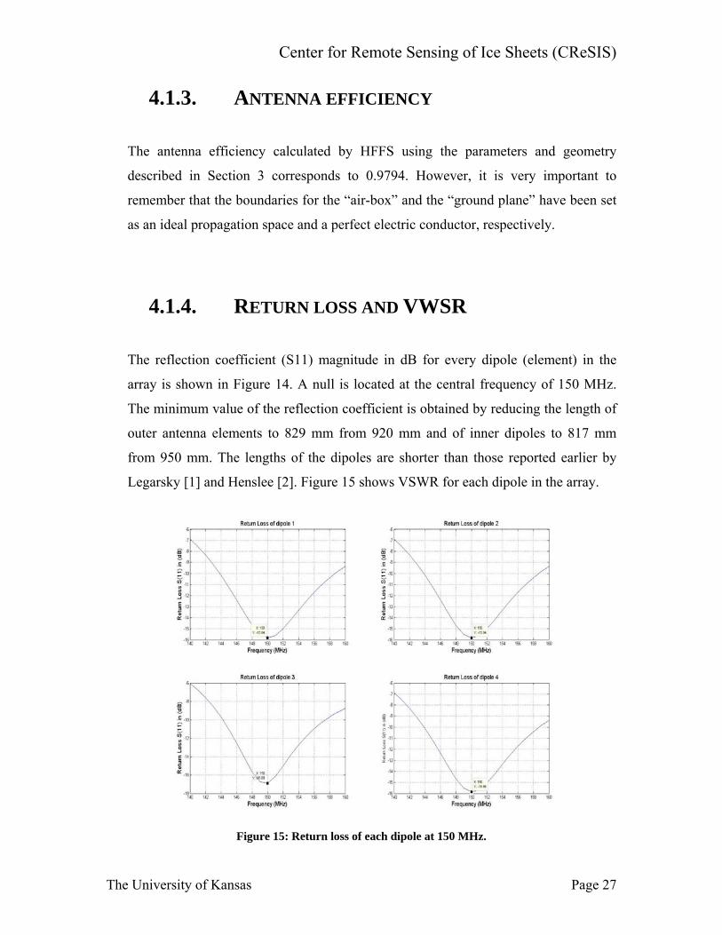
4.1.3. Antenna efficiency ........................................................................................ 27

4.1.4. Return loss and VWSR ................................................................................. 27

4.2. Simulations at 450 MHz ................................................................................... 28

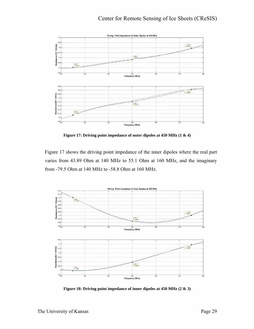
4.2.1. Driving point impedance............................................................................... 28

4.2.2. Far field radiation pattern.............................................................................. 30

4.2.2.1. 3-D Far field radiation pattern .................................................................. 32

4.2.3. Antenna efficiency ........................................................................................ 32

4.2.4. Return loss and VWSR ................................................................................. 33

5. Antenna Measurement results................................................................................... 35

5.1. results at 450 MHz............................................................................................ 36

5.2. results at 1350 MHz (1.35 GHz)....................................................................... 38

6. Conclusions............................................................................................................... 39

The University of Kansas Page 2


Table of Figures

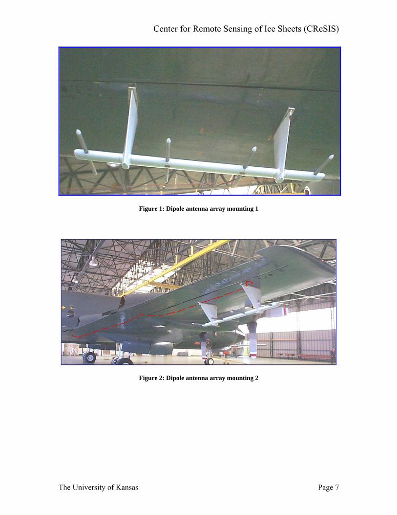
Figure 1: Dipole antenna array mounting 1 ........................................................................ 7

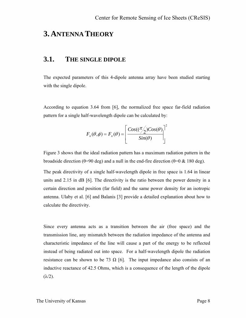
Figure 2: Dipole antenna array mounting 2 ........................................................................ 7

Figure 3: Far-Field Radiation pattern for a single dipole. .................................................. 9

Figure 4: Front and side views of the dipole array composed of four true dipoles and

images. .............................................................................................................................. 10

Figure 5: Dipole positioning for mutual coupling. ........................................................... 13

Figure 6: Four-dipole antenna array at 150 [MHz]........................................................... 15

Figure 7: Balun configuration........................................................................................... 18

Figure 8: GISMO antenna array configuration................................................................. 19

Figure 9: Driving point impedance of outer dipoles at 150 MHz (1 & 4) ........................ 23

Figure 10: Driving point impedance of inner dipoles at 150MHz (2 & 3) ....................... 24

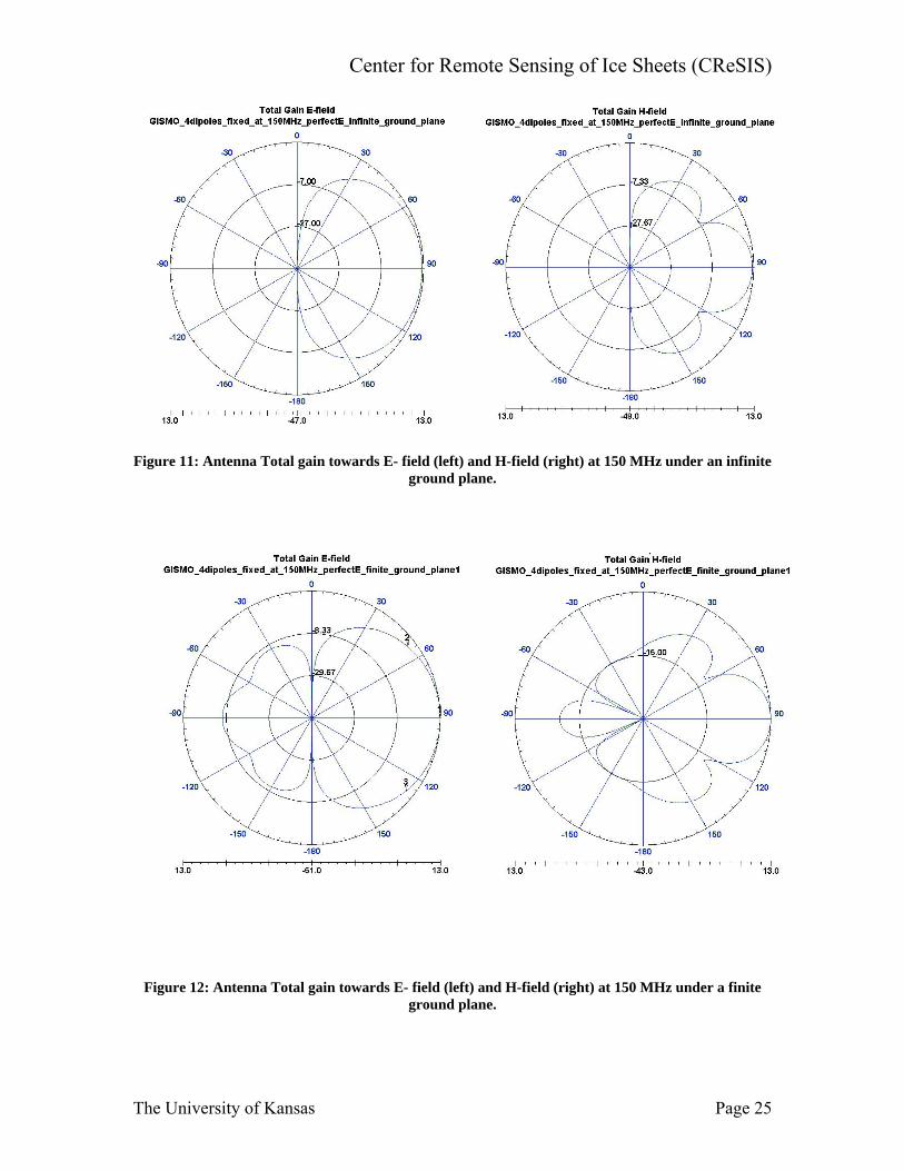
Figure 11: Antenna Total gain towards E- field (left) and H-field (right) at 150 MHz

under an infinite ground plane. ......................................................................................... 25

Figure 12: Antenna Total gain towards E- field (left) and H-field (right) at 150 MHz

under a finite ground plane. .............................................................................................. 25

Figure 13: Antenna gain towards E-field (left) and H-field (right) at 150 MHz under a

finite ground plane with weighting. .................................................................................. 26

Figure 14: Antenna 3-D gain at 150 MHz under an infinite ground plane....................... 26

Figure 15: Return loss of each dipole at 150 MHz. .......................................................... 27

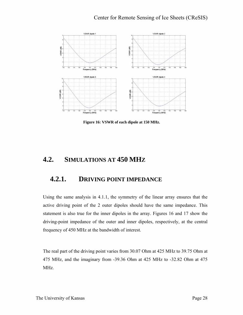
Figure 16: VSWR of each dipole at 150 MHz.................................................................. 28

Figure 17: Driving point impedance of outer dipoles at 450 MHz (1 & 4) ...................... 29

Figure 18: Driving point impedance of inner dipoles at 450 MHz (2 & 3) ...................... 29

Figure 19: Antenna Total gain towards E-field (left) and H-field (right) at 450 MHz under

an infinite ground plane. ................................................................................................... 30

Figure 20: Antenna Total gain towards E-field (left) and H-field (right) at 450 MHz under

a finite ground plane. ........................................................................................................ 31

Figure 21: Antenna gain towards E-field (left) and H-field (right) at 450 MHz under a

finite ground plane with weighting. .................................................................................. 31



Figure 22: Antenna 3-D gain at 450 MHz under an infinite ground plane....................... 32

Figure 23: Return loss of each dipole at 450 MHz. .......................................................... 33

Figure 24: VSWR of each dipole at 450 MHz.................................................................. 34

Figure 25: Mini-Circuits ZB4PD1-500 power combiner used at 450 MHz. .................... 35

Figure 26: Mini-Circuits ZB8PD-2 power combiner used at 1350 MHz. ........................ 36

Figure 27: Return loss of the array when outer dipoles are shorter (left), and when inner

dipoles are shorter (right).................................................................................................. 37

Figure 28: Return loss of the array when dipoles have the simulated length. .................. 37

Figure 29: Return loss at 450 MHz when outer dipoles are 265 mm or 10.4 in and inner

dipoles are 261 mm or 10.2 in. ......................................................................................... 38



1. ABSTRACT

The Glaciers and Ice Sheets Mapping Orbiter (GISMO) radar project proposes to

develop and demonstrate a novel concept for measuring the surface and basal

topography of terrestrial ice sheets. It will also determine the physical properties of

the glacier bed. The primary goal of the project is to develop and demonstrate

methods for isolating returns from the ice-bed interface from those from the ice

surface. As its role in this project, the Center for Remote Sensing of Ice Sheets

(CReSIS) is developing a radar that operates at 150 MHz with a bandwidth of 20

MHz and at 450 MHz with a bandwidth of 50MHz. It will collect data with a multi-

phase-center antenna to test interferometric phase filtering and tomographic

techniques to isolate returns from the ice bed and ice surface.

This report describes the design, simulation and test of antenna arrays for GISMO

radar. The work described in the report is carried out as a part of a graduate directed

reading course.

The simulations outlined in this report at both center frequencies exhibit results that

are in contrast to previous studies. The length of the dipoles needs to be resized to

obtain a lower return loss than that reported earlier. Also, to achieve return loss of the

antenna array below -10 dB over wider bandwidth, the outer dipoles (1 and 4) should

be longer than the inner ones (2 and 3). This is exactly opposite to what was reported

in the previous studies [1, 2].

Finally, a test conducted over a 1:3 scale-model antenna array, validates the need to

resize the dipole’s length to obtain lower return loss as simulated. With a few minor

modifications to the existing antenna array for the NASA P-3 aircraft, the results can

meet project requirements.



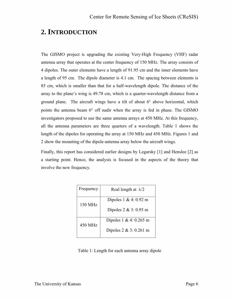
2. INTRODUCTION

The GISMO project is upgrading the existing Very-High Frequency (VHF) radar

antenna array that operates at the center frequency of 150 MHz. The array consists of

4 dipoles. The outer elements have a length of 91.95 cm and the inner elements have

a length of 95 cm. The dipole diameter is 4.1 cm. The spacing between elements is

85 cm, which is smaller than that for a half-wavelength dipole. The distance of the

array to the plane’s wing is 49.78 cm, which is a quarter-wavelength distance from a

ground plane. The aircraft wings have a tilt of about 6° above horizontal, which

points the antenna beam 6° off nadir when the array is fed in phase. The GISMO

investigators proposed to use the same antenna arrays at 450 MHz. At this frequency,

all the antenna parameters are three quarters of a wavelength. Table 1 shows the

length of the dipoles for operating the array at 150 MHz and 450 MHz. Figures 1 and

2 show the mounting of the dipole-antenna array below the aircraft wings.

Finally, this report has considered earlier designs by Legarsky [1] and Henslee [2] as

a starting point. Hence, the analysis is focused in the aspects of the theory that

involve the new frequency.

Frequency Real length at λ/2

150 MHz Dipoles 1 & 4: 0.92 m

Dipoles 2 & 3: 0.95 m

450 MHz Dipoles 1 & 4: 0.265 m

Dipoles 2 & 3: 0.261 m

Table 1: Length for each antenna array dipole



Figure 1: Dipole antenna array mounting 1

Figure 2: Dipole antenna array mounting 2



3. ANTENNA THEORY

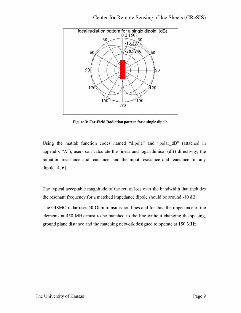
3.1. THE SINGLE DIPOLE

The expected parameters of this 4-dipole antenna array have been studied starting

with the single dipole.

According to equation 3.64 from [6], the normalized free space far-field radiation

pattern for a single half-wavelength dipole can be calculated by:

2

)(

)()2(()(),(

⎥⎥

⎦

⎤

⎢⎢

⎣

⎡==

θ

θπθφθ

Sin

CosCosFF nn

Figure 3 shows that the ideal radiation pattern has a maximum radiation pattern in the

broadside direction (θ=90 deg) and a null in the end-fire direction (θ=0 & 180 deg).

The peak directivity of a single half-wavelength dipole in free space is 1.64 in linear

units and 2.15 in dB [6]. The directivity is the ratio between the power density in a

certain direction and position (far field) and the same power density for an isotropic

antenna. Ulaby et al. [6] and Balanis [3] provide a detailed explanation about how to

calculate the directivity.

Since every antenna acts as a transition between the air (free space) and the

transmission line, any mismatch between the radiation impedance of the antenna and

characteristic impedance of the line will cause a part of the energy to be reflected

instead of being radiated out into space. For a half-wavelength dipole the radiation

resistance can be shown to be 73 Ω [6]. The input impedance also consists of an

inductive reactance of 42.5 Ohms, which is a consequence of the length of the dipole

(λ/2).



Figure 3: Far-Field Radiation pattern for a single dipole.

Using the matlab function codes named “dipole” and “polar_dB” (attached in

appendix “A”), users can calculate the linear and logarithmical (dB) directivity, the

radiation resistance and reactance, and the input resistance and reactance for any

dipole [4, 6].

The typical acceptable magnitude of the return loss over the bandwidth that includes

the resonant frequency for a matched impedance dipole should be around -10 dB.

The GISMO radar uses 50-Ohm transmission lines and for this, the impedance of the

elements at 450 MHz must to be matched to the line without changing the spacing,

ground plane distance and the matching network designed to operate at 150 MHz.



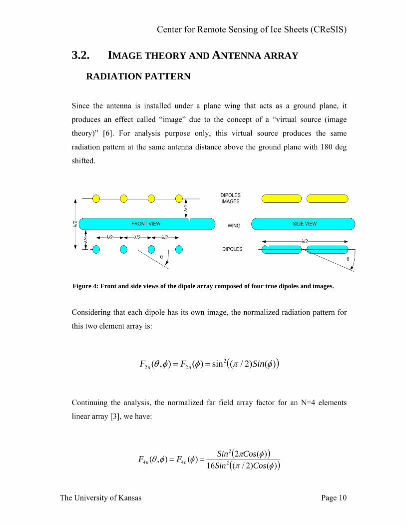
3.2. IMAGE THEORY AND ANTENNA ARRAY

RADIATION PATTERN

Since the antenna is installed under a plane wing that acts as a ground plane, it

produces an effect called “image” due to the concept of a “virtual source (image

theory)” [6]. For analysis purpose only, this virtual source produces the same

radiation pattern at the same antenna distance above the ground plane with 180 deg

shifted.

Figure 4: Front and side views of the dipole array composed of four true dipoles and images.

Considering that each dipole has its own image, the normalized radiation pattern for

this two element array is:

( ))()2/(sin)(),( 222 φπφφθ SinFF nn ==

Continuing the analysis, the normalized far field array factor for an N=4 elements

linear array [3], we have:

( )( ))()2/(16

)(2)(),( 2

2

44 φπφπφφθ

CosSinCosSinFF nn ==



Then, finally we can equate and conclude that the 4-elements antenna array radiation

pattern can be calculated by:

)()()(),( 424 φφθφθ nnnn FFFF =

( ) ( )( ))()2/(16

)(2)()2/(sin)(

)()2((),( 2

22

2

4 φπφπφπ

θ

θπφθ

CosSinCosSinSin

Sin

CosCosF n ××

⎥⎥

⎦

⎤

⎢⎢

⎣

⎡=

3.3. ANTENNA MUTUAL IMPEDANCE

The previous section describes a single-dipole resistance and input impedance.

However, since this report explains the response of a 4-dipole antenna array, it’s very

important to extend this analysis to include self and mutual impedance of the antenna

array elements.

When an antenna is in the presence of an obstacle or other element, the current

distribution, the field radiation, is altered. As a consequence of this interaction, the

input impedance of the antenna varies. The interaction between elements is referred

to as driving-point impedance and is the combination of the self-impedance and the

mutual impedance between the driven element and the other obstacles or elements.

The driving-point impedance depends upon the antenna type, the relative placement

of the elements, and the type of feed used to excite the elements.



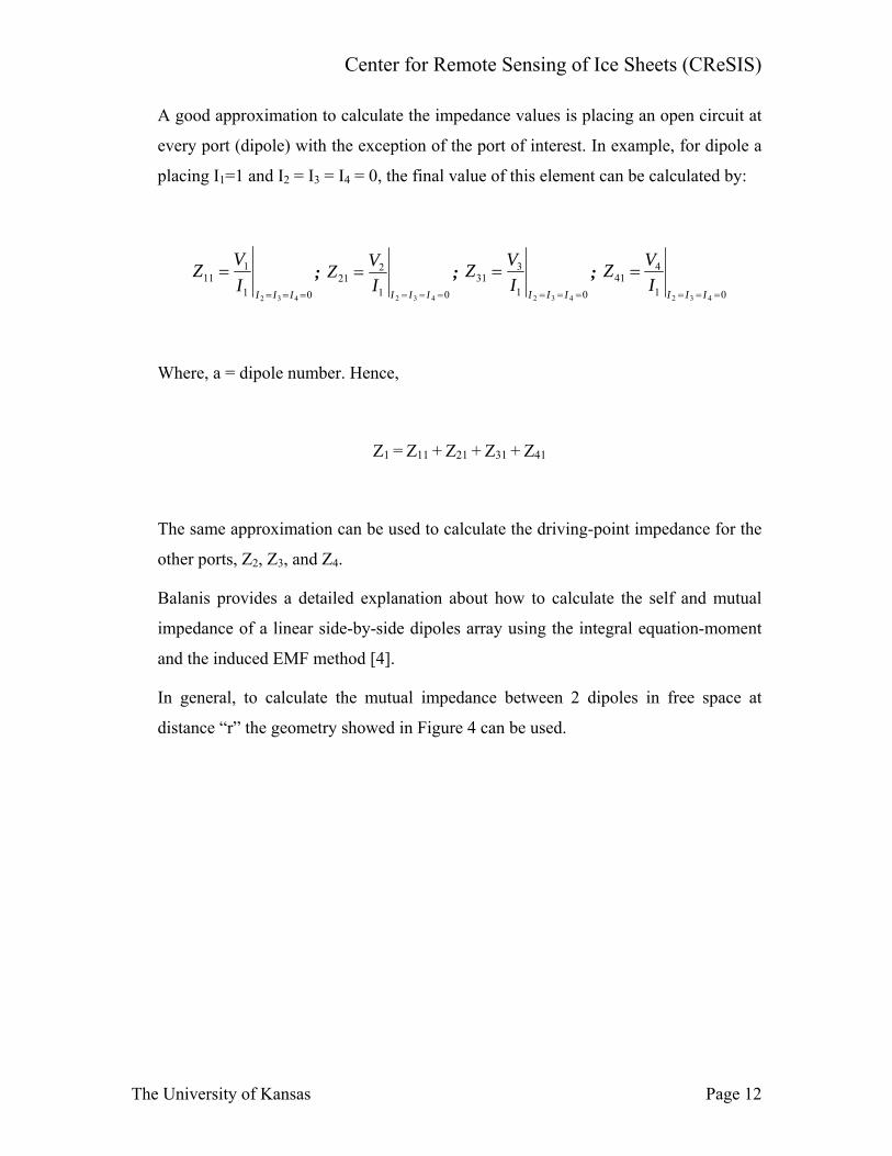
A good approximation to calculate the impedance values is placing an open circuit at

every port (dipole) with the exception of the port of interest. In example, for dipole a

placing I1=1 and I2 = I3 = I4 = 0, the final value of this element can be calculated by:

01

111

432 ===

=IIII

VZ ; 01

221

432 ===

=IIII

VZ ; 01

331

432 ===

=IIII

VZ ; 01

441

432 ===

=IIII

VZ

Where, a = dipole number. Hence,

Z1 = Z11 + Z21 + Z31 + Z41

The same approximation can be used to calculate the driving-point impedance for the

other ports, Z2, Z3, and Z4.

Balanis provides a detailed explanation about how to calculate the self and mutual

impedance of a linear side-by-side dipoles array using the integral equation-moment

and the induced EMF method [4].

In general, to calculate the mutual impedance between 2 dipoles in free space at

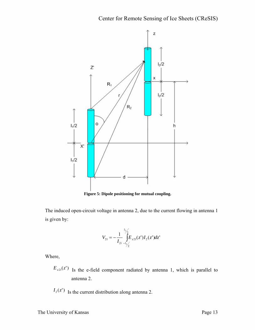
distance “r” the geometry showed in Figure 4 can be used.



Figure 5: Dipole positioning for mutual coupling.

The induced open-circuit voltage in antenna 2, due to the current flowing in antenna 1

is given by:

')'()'(1 2

2

2212

21

2

2

dzzIzEI

V

l

lz

i∫

−

−=

Where,

)'(21 zE z Is the e-field component radiated by antenna 1, which is parallel to

antenna 2.

)'(2 zI Is the current distribution along antenna 2.



Therefore, the mutual impedance can be expressed as:

')'()'(1 2

2

221211

221

2

2

dzzIzEIII

VZ

l

lz

iii

li ∫

−

−==

3.4. ANTENNA MUTUAL COUPLING

Whether two or more antennas, near each other, are active (transmitting) or passive

(receiving), some of the energy of each one will be induced in the others. In general,

the amount of energy induced in an antenna array will depend on four factors: the

radiation characteristics of each, the relative separation between them, the relative

orientation of each, and the scan volume of the array. The effect of this induced

energy over a passive element when the antennas in the array are transmitting is

called coupling.

The coupling effect is the relative change of the driving impedance of each element,

and it is usually called mutual impedance driving [3]. For better understanding, we

have adopted the following terminology:

Antenna impedance: The impedance looking into a single insolated element.

Passive driving impedance: The impedance looking into a single element of

an array with all other elements of the array passively terminated in their

normal generator impedance

Active driving impedance: The impedance looking into a single element of an

array with all other elements excited



While passive driving impedance has a minor influence in the antenna impedance, we

will assume that driving impedance would refer to active driving impedance.

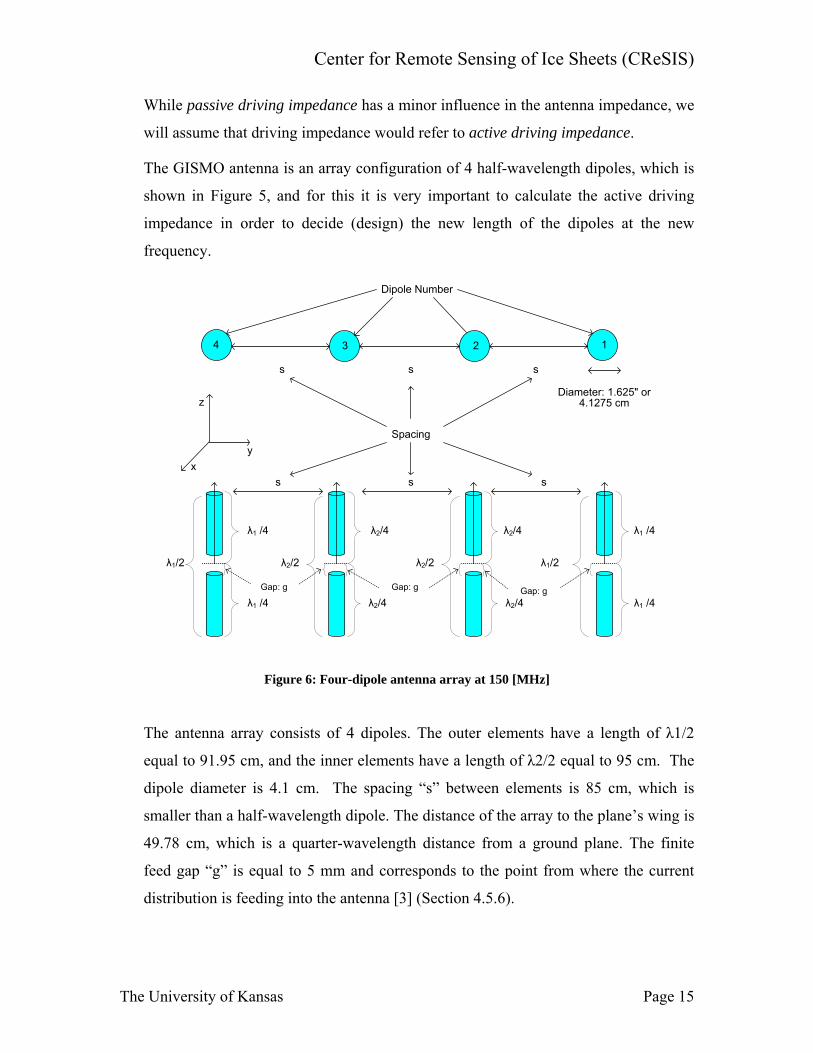
The GISMO antenna is an array configuration of 4 half-wavelength dipoles, which is

shown in Figure 5, and for this it is very important to calculate the active driving

impedance in order to decide (design) the new length of the dipoles at the new

frequency.

s s s

1234

Dipole Number

Spacing

s ss

λ2/2 λ1/2

z

yx

Diameter: 1.625" or 4.1275 cm

λ1 /4

Gap: g

λ2/4

Gap: gGap: g

λ1 /4

λ1 /4

λ1 /4

λ1/2

λ2/4

λ2/4

λ2/4

λ2/2

Figure 6: Four-dipole antenna array at 150 [MHz]

The antenna array consists of 4 dipoles. The outer elements have a length of λ1/2

equal to 91.95 cm, and the inner elements have a length of λ2/2 equal to 95 cm. The

dipole diameter is 4.1 cm. The spacing “s” between elements is 85 cm, which is

smaller than a half-wavelength dipole. The distance of the array to the plane’s wing is

49.78 cm, which is a quarter-wavelength distance from a ground plane. The finite

feed gap “g” is equal to 5 mm and corresponds to the point from where the current

distribution is feeding into the antenna [3] (Section 4.5.6).



3.5. ANTENNA IMPEDANCE MATCHING

Based on the material and physical dimensions, every antenna has its own

characteristic impedance. However, this does not always match the impedance of the

transmitters, receivers and transmission lines. This difference produces an undesired

reflection of the power when an antenna is feeding. Matching networks are used to

match the impedance between the antenna and connected transmission line in order to

minimize the power reflection. Factors that should be considered in a matching

network design include: complexity, bandwidth, implementation and adjustability [5].

There are different kinds of matching networks and the most common are: L-

networks, single-stub tuning (shunt and series), double-stub, quarter-wave

transformers, binomial multi-section transformers, Chebyshev multi-section

transformers, and tapered lines. Details of how are the performance of these matching

networks can be implemented are described by [5].

Very often, when an engineer can not modify a matching network (GISMO 4-dipole

antenna array), a good approximation for tuning the antenna is resizing the length of

the dipoles until the input impedance matches the transmission line impedance. The

GISMO antenna design has an L-section matching network implemented by 3

elements: an air coil for the inductor, the air dielectric, and a trimmer for the capacitor

[1]. However, since the GISMO antenna has to work at 150 MHz and 450 MHz, the

original matching network implemented for the first frequency will not work for the

second and the matching network might not be needed. Hence, this report doesn’t

demonstrate the response of a new matching network. Furthermore, it’s important to

remember that a dipole radiation resistance at the input terminal is 73 Ohms. Also, the

imaginary part (reactance) associated with the input impedance for a dipole is a

function of its length, and for l =λ/2 this reactance is equal to 42.5*j Ohms. In order

to reduce the imaginary part of the input impedance to zero, the antenna (dipole) is

matched or reduced in length until the reactance vanishes [3], which is the case in this

analysis since we are not allowed to change or install a new matching network in the

antenna.



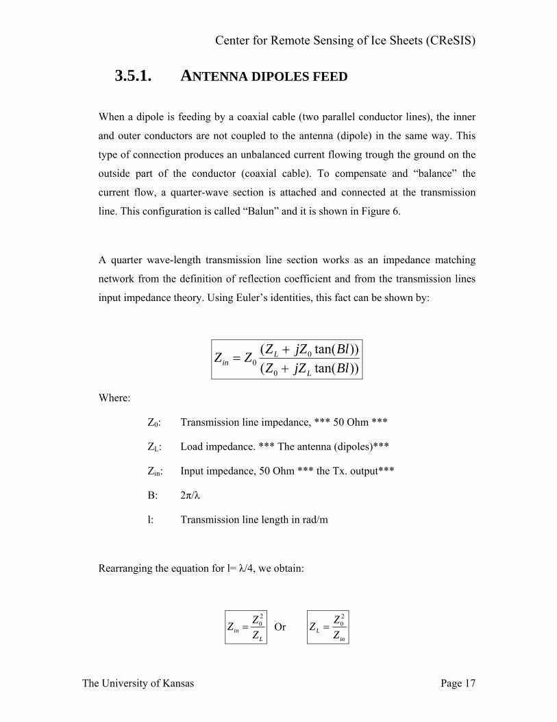
3.5.1. ANTENNA DIPOLES FEED

When a dipole is feeding by a coaxial cable (two parallel conductor lines), the inner

and outer conductors are not coupled to the antenna (dipole) in the same way. This

type of connection produces an unbalanced current flowing trough the ground on the

outside part of the conductor (coaxial cable). To compensate and “balance” the

current flow, a quarter-wave section is attached and connected at the transmission

line. This configuration is called “Balun” and it is shown in Figure 6.

A quarter wave-length transmission line section works as an impedance matching

network from the definition of reflection coefficient and from the transmission lines

input impedance theory. Using Euler’s identities, this fact can be shown by:

))tan(())tan((

0

00 BljZZ

BljZZZZL

Lin +

+=

Where:

Z0: Transmission line impedance, *** 50 Ohm ***

ZL: Load impedance. *** The antenna (dipoles)***

Zin: Input impedance, 50 Ohm *** the Tx. output***

B: 2π/λ

l: Transmission line length in rad/m

Rearranging the equation for l= λ/4, we obtain:

Lin Z

ZZ20= Or

inL Z

ZZ20=



These equations tells us that if ZL >>>>Z02 then Zin is very small and in consequence

acts as a short circuit. The opposite statement is also true. When Zin >>>>Z02 then ZL

is very small and in consequence acts as a short circuit, and the opposite statement is

also true.

Figure 7: Balun configuration.

The GISMO balun (balance) short circuit between the transmission line shield and the

quarter-wave wire has been placed at the 94.5% length of the last one.

3.6. GRATING LOBES

When two or more antenna elements are placed in an array, the spacing or distance

between them is very important in terms of the radiation field. That is, if the spacing

between elements is greater or equal to the half-wavelength at the central frequency,



multiple lobes at the same magnitude of the main lobe can be formed [3]. Grating

lobes are defined as the other lobes instead of the main ones. These grating lobes are

the result of large spacing between elements to permit in-phase addition of the

radiation field in more than one direction. To avoid grating lobes, the spacing

between elements should be less than a half-wavelength. This condition has to be

accomplished whether the array is in linear or planar configuration [3]. However, the

grating lobes for GISMO may not be a problem because the imaging is confined to

incidence of less than 20 degrees.

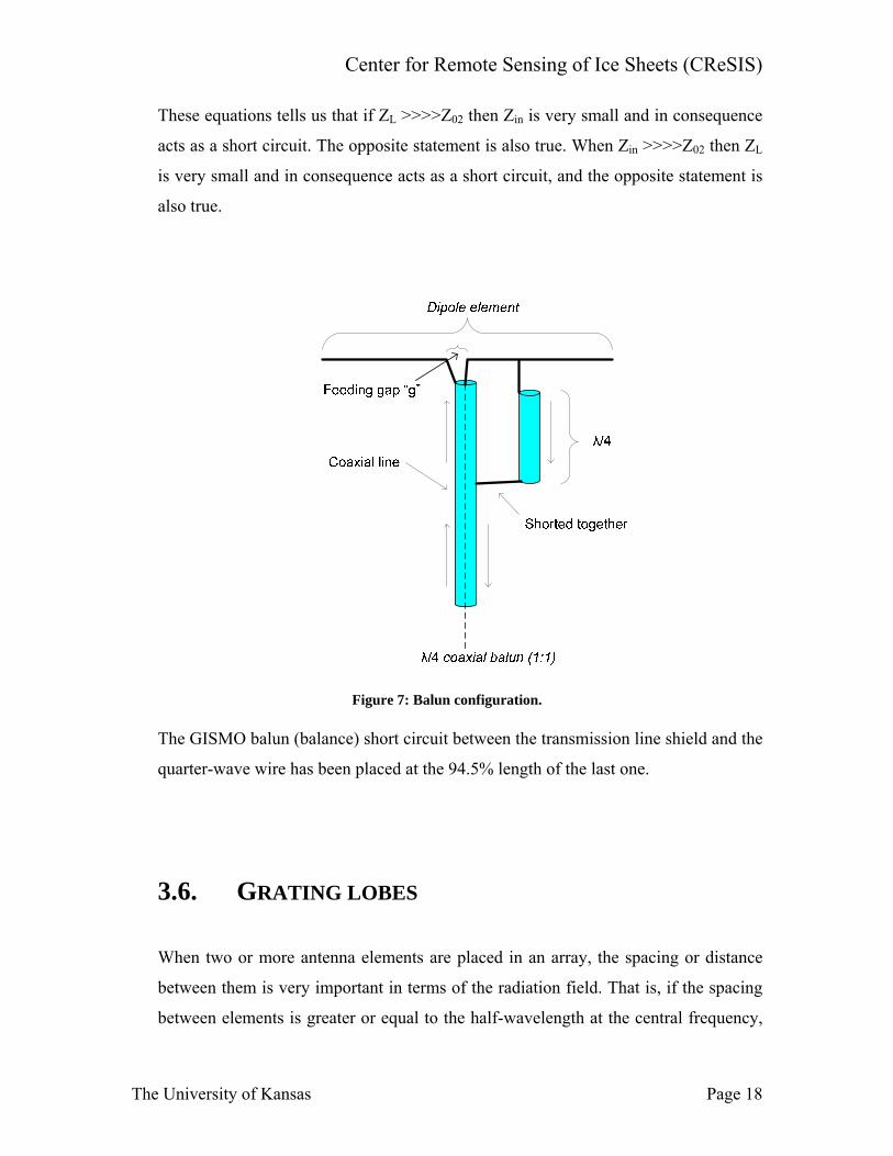
The GISMO antenna array is a linear configuration and the spacing between elements

has been set up at less than a half-wavelength at 150 MHz as a central frequency. In

effect, the spacing between elements is 85 cm, as Figure 7 shows.

Unfortunately, since the GISMO radar has been designed to work at two different

frequencies, the spacing between elements designed at the central frequency of 150

MHz is larger than a half-wavelength when the radar operates at the central frequency

of 450 MHz. Grating lobes at 450 MHz are the consequence.

Figure 8: GISMO antenna array configuration.



3.7. ANTENNA EFFICIENCY

The most common definition for “antenna efficiency” (e0) is the ratio between the

power radiated from the antenna and the power input in its terminals. There is a

reflection due to a mismatch between the antenna and the transmission line, and the

dielectric and conductive properties of the material (I2R), and it is very important to

remember that these factors must be considered when calculating the radiation

efficiency.

In general terms, and as Balanis [3] writes in Chapter 2, the overall efficiency can be

written as:

dcr eeee =0

Where,

e0 = total efficiency (dimensionless)

er = reflection efficiency = (1-|Γ|2) (dimensionless)

ec = conduction efficiency

ed = dielectric efficiency

Γ = voltage reflection coefficient at the input terminal of the antenna



4. ANTENNA SIMULATION RESULTS

The GISMO antenna array has been simulated at 2 central frequencies, 150 MHz and

450 MHz, using the software High Frequency Structure Simulator (HFFS) version 10

by Ansoft Corporation. The results were exported to Matlab version 7 for better

analysis, based on a computer with 1 GB-Ram at 2.4 GHz CPU. The parameters for

the 4-dipole antenna array have been set up with the following configuration:

1. Model (Geometry) : According to Figure 7

2. Dipoles Thickness : 3.302 mm

3. Boundaries : Perfect E infinite ground plane over the

array at λ/4

4. Excitations : Lumped ports at 50 Ohm, which is the

transmission line impedance.

5. Analysis : Central frequency at 150 MHz with a sweep

between 140 to 160 MHz, and at the central

frequency 450 MHz with a sweep between

425 to 475 MHz.

6. Radiation

a. E-field : Type infinite sphere.

i. Start theta : -180 degree.

ii. Stop theta : 180 degree.

iii. Theta step : 1 degree.

iv. Start Phi : 90 degree.

v. Stop Phi : 90 degree.

vi. Phi step : 1 degree.



b. H-field : Type infinite sphere.

i. Start theta : 90 degree.






c. Infinite sphere : Type infinite sphere.

i. Start theta : 0 degree.






4.1. SIMULATIONS AT 150 MHZ

4.1.1. DRIVING POINT IMPEDANCE

Since GISMO antenna is a symmetrical linear array, and in agreement with [2], the

active driving point of the outer dipoles should have the same impedance. This

statement is also true for the inner dipoles of the array. However, the simulation

conducted in the present report shows that inner dipoles have to be shorter than outer

dipoles. This contradicts earlier results reported by Legarsky [2] and is later



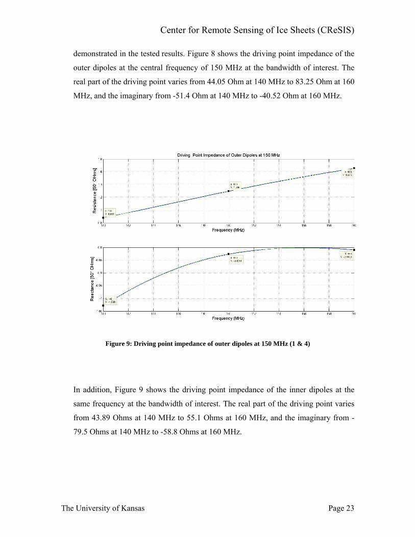
demonstrated in the tested results. Figure 8 shows the driving point impedance of the

outer dipoles at the central frequency of 150 MHz at the bandwidth of interest. The

real part of the driving point varies from 44.05 Ohm at 140 MHz to 83.25 Ohm at 160

MHz, and the imaginary from -51.4 Ohm at 140 MHz to -40.52 Ohm at 160 MHz.

Figure 9: Driving point impedance of outer dipoles at 150 MHz (1 & 4)

In addition, Figure 9 shows the driving point impedance of the inner dipoles at the

same frequency at the bandwidth of interest. The real part of the driving point varies

from 43.89 Ohms at 140 MHz to 55.1 Ohms at 160 MHz, and the imaginary from -

79.5 Ohms at 140 MHz to -58.8 Ohms at 160 MHz.



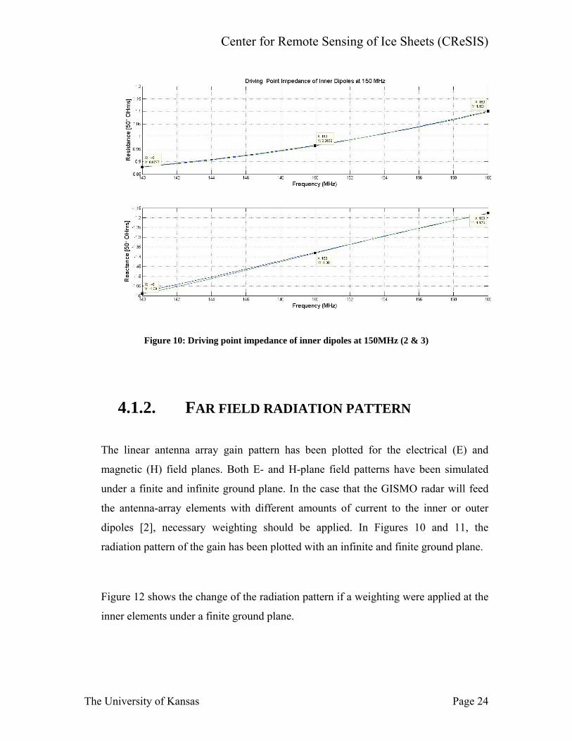
Figure 10: Driving point impedance of inner dipoles at 150MHz (2 & 3)

4.1.2. FAR FIELD RADIATION PATTERN

The linear antenna array gain pattern has been plotted for the electrical (E) and

magnetic (H) field planes. Both E- and H-plane field patterns have been simulated

under a finite and infinite ground plane. In the case that the GISMO radar will feed

the antenna-array elements with different amounts of current to the inner or outer

dipoles [2], necessary weighting should be applied. In Figures 10 and 11, the

radiation pattern of the gain has been plotted with an infinite and finite ground plane.

Figure 12 shows the change of the radiation pattern if a weighting were applied at the

inner elements under a finite ground plane.



Figure 11: Antenna Total gain towards E- field (left) and H-field (right) at 150 MHz under an infinite

ground plane.

Figure 12: Antenna Total gain towards E- field (left) and H-field (right) at 150 MHz under a finite ground plane.



Figure 13: Antenna gain towards E-field (left) and H-field (right) at 150 MHz under a finite ground plane with weighting.

4.1.2.1. 3-D FAR FIELD RADIATION PATTERN

HFSS has the capability to calculate and plot a 3D image depicting the real beam of

the gain. Figure 13 shows the total gain 3D graph for 150 MHz.

Figure 14: Antenna 3-D gain at 150 MHz under an infinite ground plane.



4.1.3. ANTENNA EFFICIENCY

The antenna efficiency calculated by HFFS using the parameters and geometry

described in Section 3 corresponds to 0.9794. However, it is very important to

remember that the boundaries for the “air-box” and the “ground plane” have been set

as an ideal propagation space and a perfect electric conductor, respectively.

4.1.4. RETURN LOSS AND VWSR

The reflection coefficient (S11) magnitude in dB for every dipole (element) in the

array is shown in Figure 14. A null is located at the central frequency of 150 MHz.

The minimum value of the reflection coefficient is obtained by reducing the length of

outer antenna elements to 829 mm from 920 mm and of inner dipoles to 817 mm

from 950 mm. The lengths of the dipoles are shorter than those reported earlier by

Legarsky [1] and Henslee [2]. Figure 15 shows VSWR for each dipole in the array.

Figure 15: Return loss of each dipole at 150 MHz.



Figure 16: VSWR of each dipole at 150 MHz.

4.2. SIMULATIONS AT 450 MHZ

4.2.1. DRIVING POINT IMPEDANCE

Using the same analysis in 4.1.1, the symmetry of the linear array ensures that the

active driving point of the 2 outer dipoles should have the same impedance. This

statement is also true for the inner dipoles in the array. Figures 16 and 17 show the

driving-point impedance of the outer and inner dipoles, respectively, at the central

frequency of 450 MHz at the bandwidth of interest.

The real part of the driving point varies from 30.07 Ohm at 425 MHz to 39.75 Ohm at

475 MHz, and the imaginary from -39.36 Ohm at 425 MHz to -32.82 Ohm at 475

MHz.



Figure 17: Driving point impedance of outer dipoles at 450 MHz (1 & 4)

Figure 17 shows the driving point impedance of the inner dipoles where the real part

varies from 43.89 Ohm at 140 MHz to 55.1 Ohm at 160 MHz, and the imaginary

from -79.5 Ohm at 140 MHz to -58.8 Ohm at 160 MHz.

Figure 18: Driving point impedance of inner dipoles at 450 MHz (2 & 3)



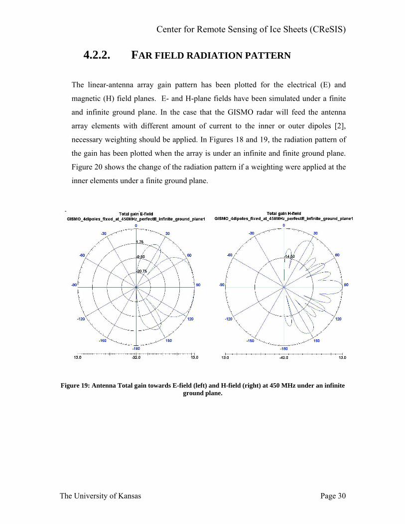
4.2.2. FAR FIELD RADIATION PATTERN

The linear-antenna array gain pattern has been plotted for the electrical (E) and

magnetic (H) field planes. E- and H-plane fields have been simulated under a finite

and infinite ground plane. In the case that the GISMO radar will feed the antenna

array elements with different amount of current to the inner or outer dipoles [2],

necessary weighting should be applied. In Figures 18 and 19, the radiation pattern of

the gain has been plotted when the array is under an infinite and finite ground plane.

Figure 20 shows the change of the radiation pattern if a weighting were applied at the

inner elements under a finite ground plane.

Figure 19: Antenna Total gain towards E-field (left) and H-field (right) at 450 MHz under an infinite ground plane.



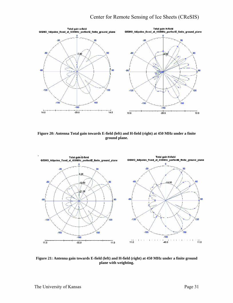
Figure 20: Antenna Total gain towards E-field (left) and H-field (right) at 450 MHz under a finite

ground plane.

Figure 21: Antenna gain towards E-field (left) and H-field (right) at 450 MHz under a finite ground

plane with weighting.



4.2.2.1. 3-D F AR FIELD RADIATION PATTERN

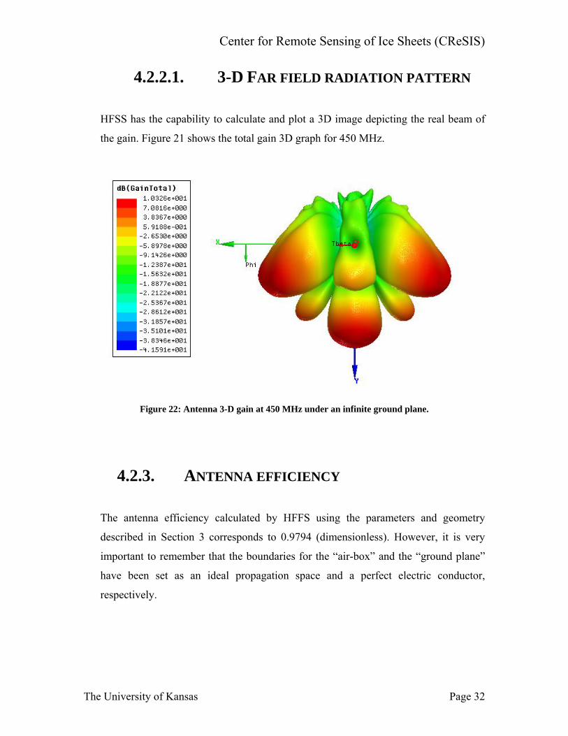
HFSS has the capability to calculate and plot a 3D image depicting the real beam of

the gain. Figure 21 shows the total gain 3D graph for 450 MHz.

Figure 22: Antenna 3-D gain at 450 MHz under an infinite ground plane.

NTENNA EFFICIENCY

The antenna efficiency calculated by HFFS using the parameters and geometry

4.2.3. A

described in Section 3 corresponds to 0.9794 (dimensionless). However, it is very

important to remember that the boundaries for the “air-box” and the “ground plane”

have been set as an ideal propagation space and a perfect electric conductor,

respectively.



4.2.4. RETURN LOSS AND VWSR

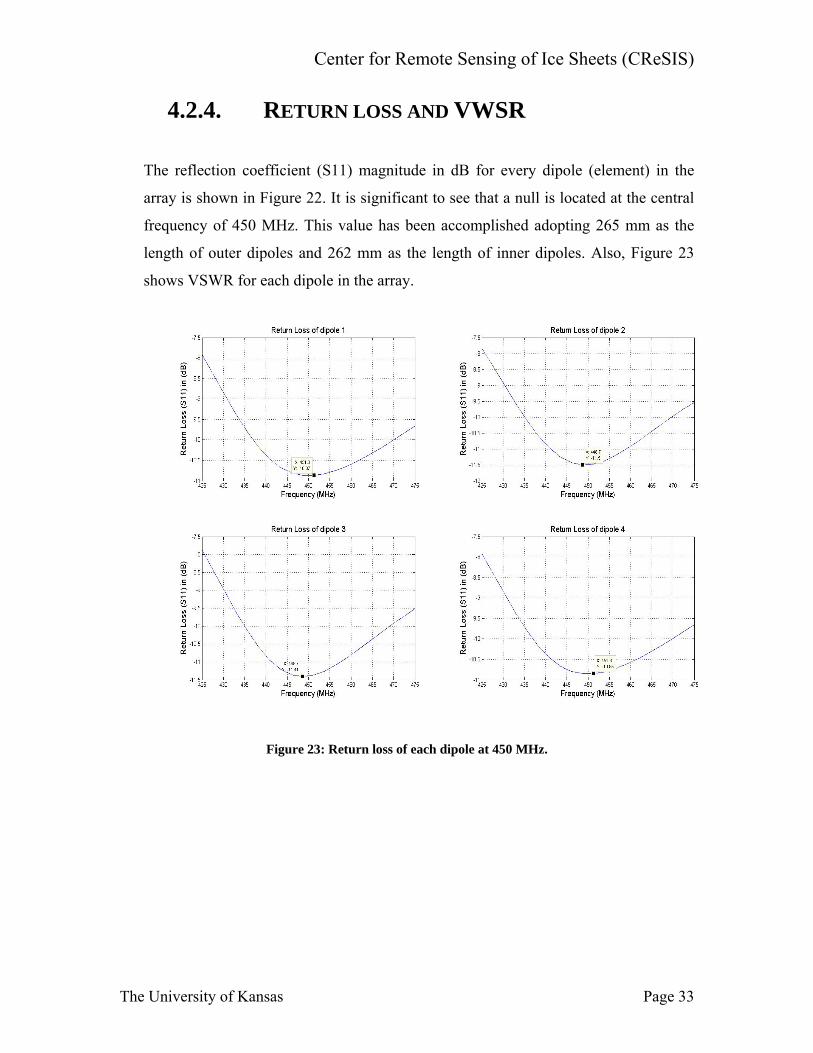
The reflection coefficient (S11) magnitude in dB for every dipole (element) in the

array is shown in Figure 22. It is significant to see that a null is located at the central

frequency of 450 MHz. This value has been accomplished adopting 265 mm as the

length of outer dipoles and 262 mm as the length of inner dipoles. Also, Figure 23

shows VSWR for each dipole in the array.

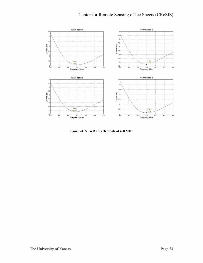
Figure 23: Return loss of each dipole at 450 MHz.



Figure 24: VSWR of each dipole at 450 MHz.



5. ANTENNA MEASUREMENT RESULTS

The GISMO antenna array has been built to scale by a factor of 3. Hence, the antenna

was tested at 450 MHz instead of 150 MHz, and at 1350 MHz (1.35 GHz) instead of

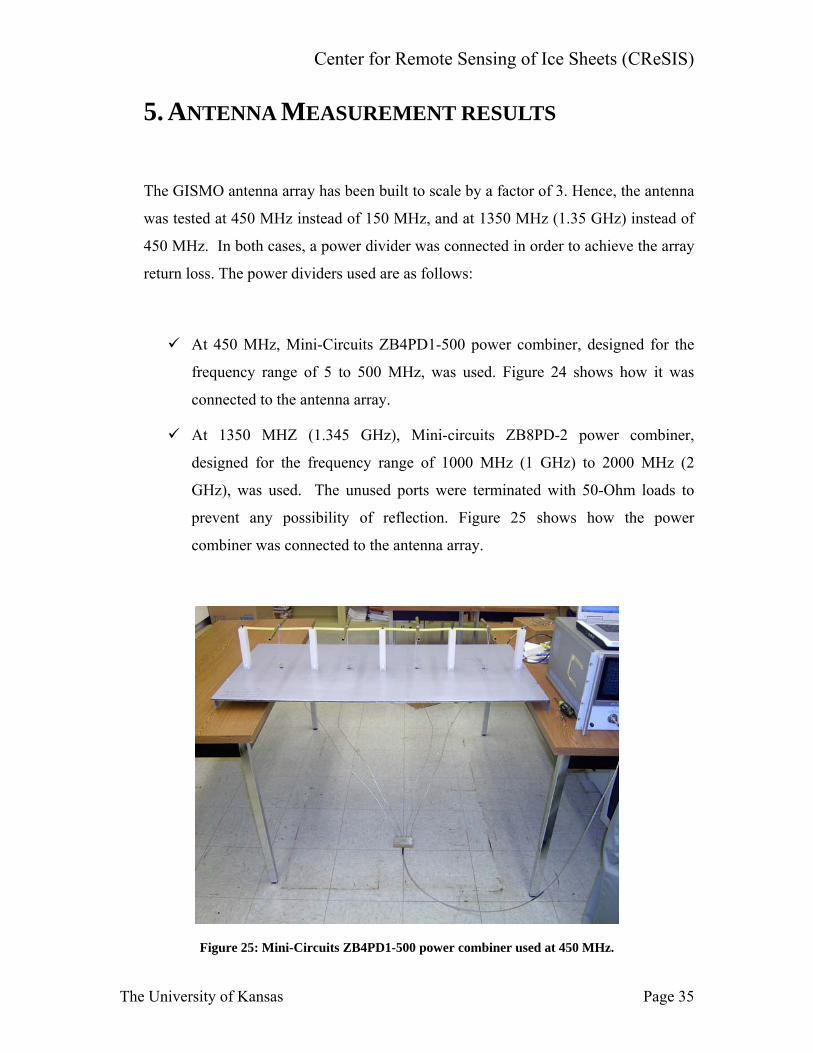
450 MHz. In both cases, a power divider was connected in order to achieve the array

return loss. The power dividers used are as follows:

At 450 MHz, Mini-Circuits ZB4PD1-500 power combiner, designed for the

frequency range of 5 to 500 MHz, was used. Figure 24 shows how it was

connected to the antenna array.

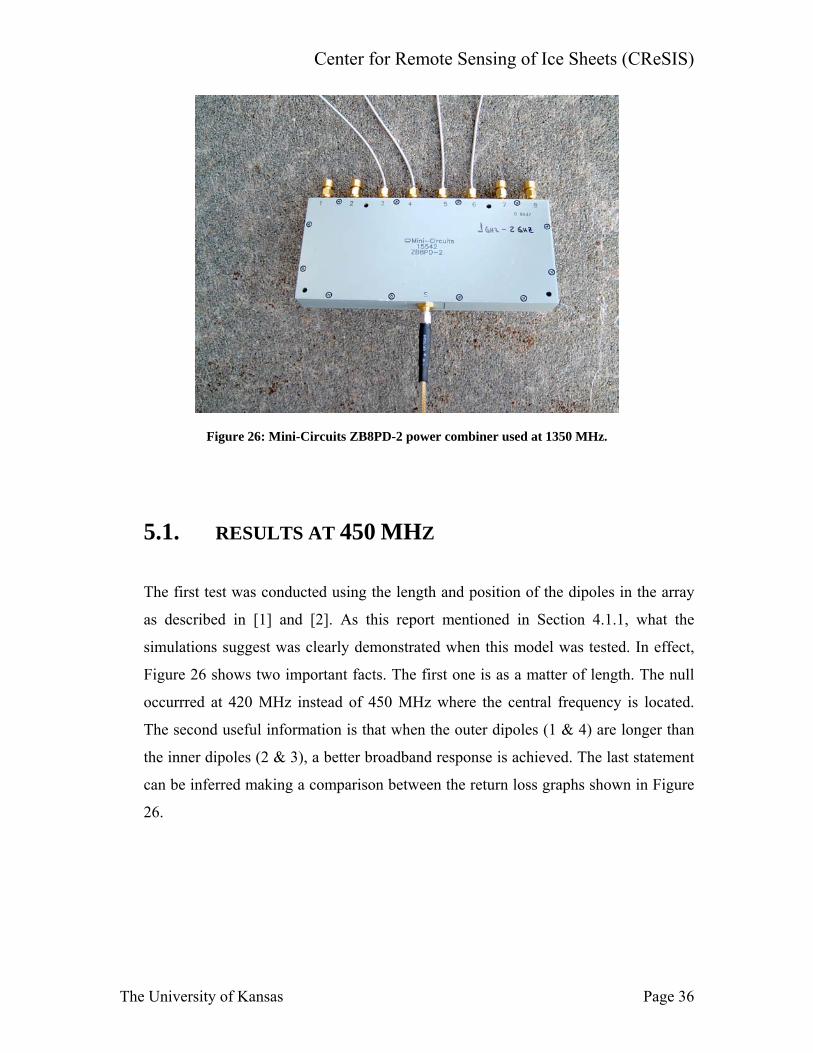
At 1350 MHZ (1.345 GHz), Mini-circuits ZB8PD-2 power combiner,

designed for the frequency range of 1000 MHz (1 GHz) to 2000 MHz (2

GHz), was used. The unused ports were terminated with 50-Ohm loads to

prevent any possibility of reflection. Figure 25 shows how the power

combiner was connected to the antenna array.

Figure 25: Mini-Circuits ZB4PD1-500 power combiner used at 450 MHz.



Figure 26: Mini-Circuits ZB8PD-2 power combiner used at 1350 MHz.

5.1. RESULTS AT 450 MHZ

The first test was conducted using the length and position of the dipoles in the array

as described in [1] and [2]. As this report mentioned in Section 4.1.1, what the

simulations suggest was clearly demonstrated when this model was tested. In effect,

Figure 26 shows two important facts. The first one is as a matter of length. The null

occurrred at 420 MHz instead of 450 MHz where the central frequency is located.

The second useful information is that when the outer dipoles (1 & 4) are longer than

the inner dipoles (2 & 3), a better broadband response is achieved. The last statement

can be inferred making a comparison between the return loss graphs shown in Figure

26.



.

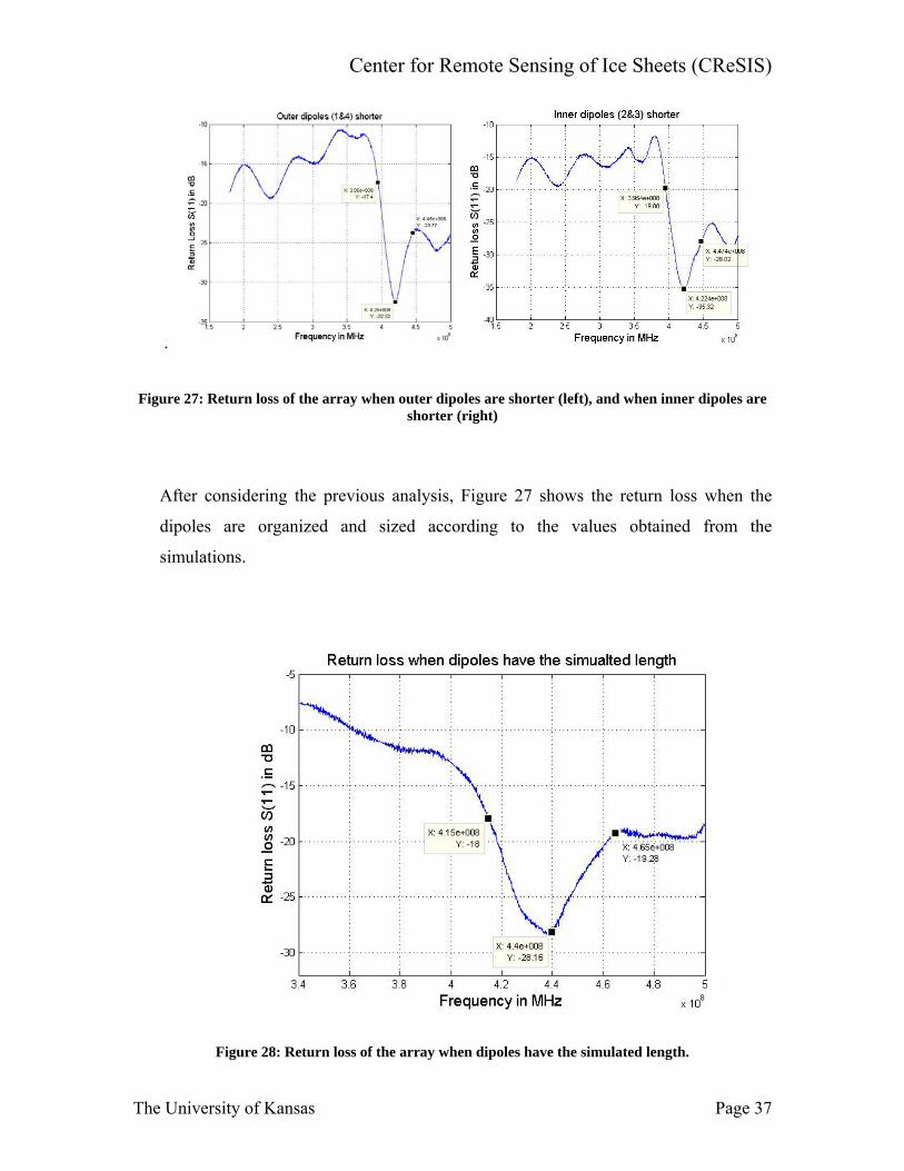
Figure 27: Return loss of the array when outer dipoles are shorter (left), and when inner dipoles are shorter (right)

After considering the previous analysis, Figure 27 shows the return loss when the

dipoles are organized and sized according to the values obtained from the

simulations.

Figure 28: Return loss of the array when dipoles have the simulated length.



5.2. RESULTS AT 1350 MHZ (1.35 GHZ)

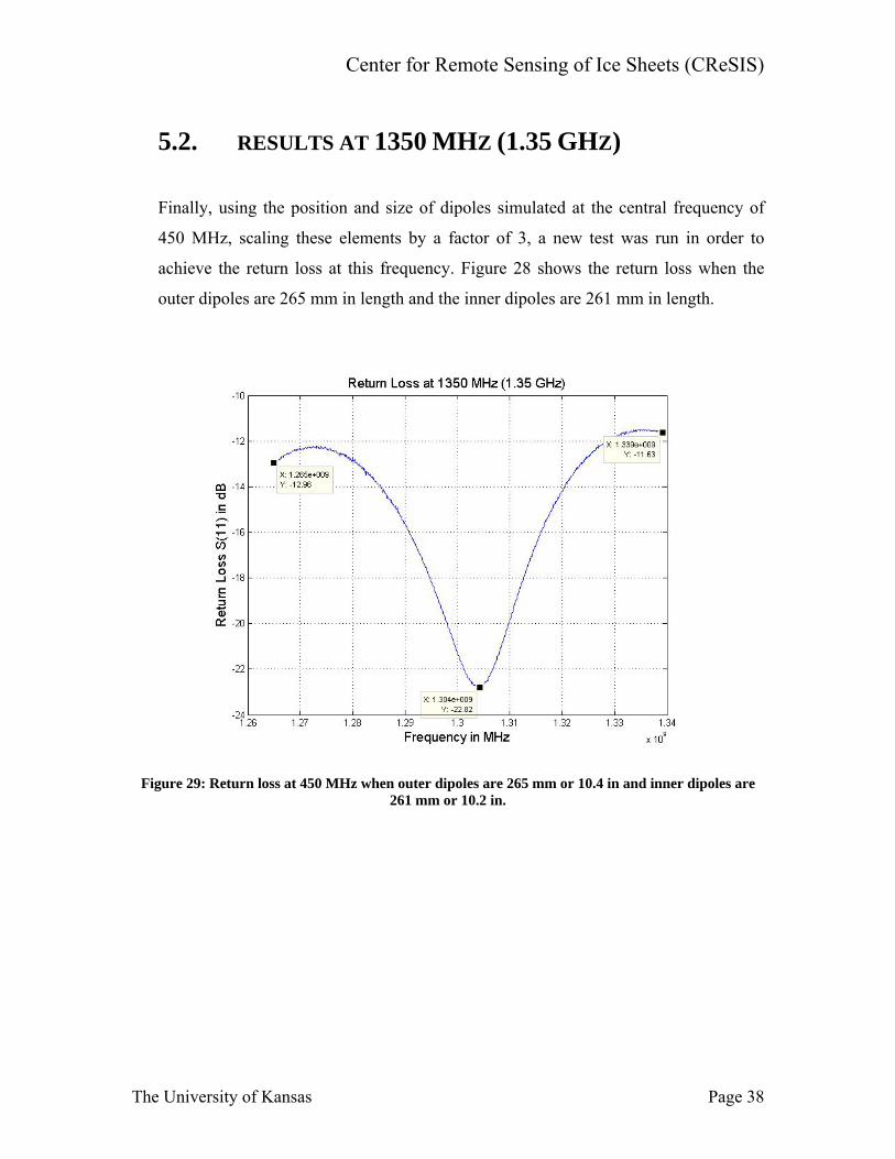
Finally, using the position and size of dipoles simulated at the central frequency of

450 MHz, scaling these elements by a factor of 3, a new test was run in order to

achieve the return loss at this frequency. Figure 28 shows the return loss when the

outer dipoles are 265 mm in length and the inner dipoles are 261 mm in length.

Figure 29: Return loss at 450 MHz when outer dipoles are 265 mm or 10.4 in and inner dipoles are 261 mm or 10.2 in.



6. CONCLUSIONS

At the central frequency of 150 MHz, contrary to [1] and [2], the outer dipoles

(1 & 4) have to be longer than inner dipoles (2 & 3). Table 2 shows the final

sizes of the antenna array dipoles at both central frequencies.

Frequency Dipoles length

150 MHz Dipoles 1 & 4: 829 mm

Dipoles 2 & 3: 0.817 mm

450 MHz Dipoles 1 & 4: 265 mm

Dipoles 2 & 3: 262 mm

Table 2: Final (tested) length for each antenna array dipole.

At the central frequency of 450 MHz, as a consequence of the distance

between elements, grating lobes with their respective side lobes appear

(Figures 18, 19 and 21). In order to eliminate grating lobes and reduce the

side lobes, the dipole spacing should be decreased to less than a half wave

length at this frequency. Unfortunately, we are not able to change the spacing

between dipoles, so we have to deal with this. In this scenario, applying

weighting to the antenna feeding point network and digital signal processing

is necessary to reduce unwanted signals.

Previous reports ([1] and [2]) described a quarter wave balun (balance) as a

feeding system for each dipole, without information about the position where

the balun is placed. This report concludes after several tests that the best result



occurs when the balun (balance) is placed at 94.5% of the quarter wave

element length from the feeding point.

References [1] Legarsky, J., Doctoral thesis, 1999

[2] Henslee, J., EECS 891 – Graduate problems report, 2003

[3] Balanis, C., Antenna Theory: Analysis and Design (Third edition), Wiley, 2005,

ISBN 0-471-66782-X

[4] Cardama, A., Jofre, L., Rius, J., Romeo, J., Blanch, S., Antenas (Spanish version),

Alfa-omega, 2000, ISBN 970-15-0454-2

[5] Pozar D., Microwave Engineering (Third edition), Wiley, 2005, ISBN 0-471-44878-8

[6] Ulaby, F., Moore, R., Fung, A., Microwave Remote Sensing Vol.I, Artechhouse,

1981, ISBN 0-89006-190-4



APPENDIX “A” Matlab codes (functions dipole and polar_dB) % ********************************************************************* % DIPOLE.m (from [3]) %********************************************************************** % This is a MATLAB based program that computes the: % I. Maximum directivity (dimensionless and in dB) % II. Radiation resistance (Rr) % III. Input resistance (Rin) % IV. Reactance relative to current maximum (Xm) % V. Input reactance (Xin) % VI. Normalized current distribution % VII. Directivity pattern (in dB) in polar form % VIII.Normalized far-field amplitude pattern (E-theta, in dB) in polar form % for a symmetrical dipole of finite length. The dipole is radiating % in free space. % % The directivity, resistances and resistances are calculated using the trailing % edge method in increments of 1 degree in theta. % % **Input parameters % 1. L: Dipole length (in wavelengths) % 2. a: Dipole radius (in wavelengths) % % **Note: % The far zone electrif field component, E-theta, exists for % 0 < theta < 180 and 0 < phi < 360. %---------------------------------------------------------------------- % function []=dipole; clear all; close all; format long; warning off; %---Choice of output--- fprintf('Output device option \n\tOption (1): Screen\n\tOption (2): File \n'); ERR = 1; while(ERR ~= 0) DEVICE = input('\nOutput device = ','s'); DEVICE = str2num(DEVICE); if(DEVICE == 1) ERR = 0; elseif(DEVICE == 2) FILNAM = input('Input the desired output filename: ','s'); ERR = 0; else error('Outputting device number should be either 1 or 2\n'); end


Center for Remote Sensing of Ice Sheets (CReSIS) end %---Definition of constants and initialization--- PI = 4.0*atan(1.0); E = 120.0*PI; THETA = PI/180.0; UMAX = 0.0; PRAD = 0.0; TOL = 1.0E-6; %---Input the length of the dipole--- L = input('\nLength of dipole in wavelengths = ','s'); L = str2num(L); %***Insert input data error loop*** r=input('Radius of dipole in wavelengths = '); %---Main program---------------------- A = L*PI; I = 1; while(I <= 180) XI = I*PI/180.0; if(XI ~= PI) U = ((cos(A*cos(XI))-cos(A))/sin(XI))^2*(E/(8.0*PI^2)); if(U > UMAX) UMAX = U; end end UA = U*sin(XI)*THETA*2.0*PI; PRAD = PRAD+UA; I = I+1; end D = (4.0*PI*UMAX)/PRAD; DDB = 10.0*log10(D); RR = 2.0*PRAD; if(A ~= PI) RIN = RR/(sin(A))^2; end %---Calculation of elevation far-field patterns in 1 degree increments--- fid = fopen('ElevPat.dat','w'); fprintf(fid,'\tDipole\n\n\tTheta\t\tE (dB)\n'); fprintf(fid,'\t----\t\t------'); T = zeros(180,1); ET = zeros(180,1); EdB = zeros(180,1);


Center for Remote Sensing of Ice Sheets (CReSIS) x = 1; while(x<=180) T(x) = x-0.99; ET(x) = (cos(PI*L*cos(T(x)*THETA))-cos(PI*L))/sin(T(x)*THETA); x = x+1; end ET = abs(ET); ETmax = max(abs(ET)); EdB = 20*log10(abs(ET)/ETmax); x = 1; while(x<=180) fprintf(fid,'\n %5.4f %12.4f',T(x),EdB(x)); x = x+1; end fclose(fid); n=120*pi; k=2*pi; if exist('cosint')~=2, disp(' '); disp('Symbolic toolbox is not installed. Switching to numerical computation of sine and cosine integrals.'); Xm=30*(2*si(k*L)+cos(k*L)*(2*si(k*L)-si(2*k*L))- ... sin(k*L)*(2*ci(k*L)-ci(2*k*L)-ci(2*k*r^2/L))); Xin=Xm/(sin(k*L/2))^2; elseif exist('cosint')==2, Xm=30*(2*sinint(k*L)+cos(k*L)*(2*sinint(k*L)-sinint(2*k*L))- ... sin(k*L)*(2*cosint(k*L)-cosint(2*k*L)-cosint(2*k*r^2/L))); Xin=Xm/(sin(k*L/2))^2; end; %---Create output------------ if(DEVICE == 2) fid = fopen(FILNAM,'w'); else fid = DEVICE; end %---Echo input parameters and output computed parameters--- fprintf(fid,'\nDIPOLE:\n-------'); fprintf(fid,'\n\nInput parameters:\n-----------------'); fprintf(fid,'\nLength of dipole in wavelengths = %6.4f',L); fprintf(fid,'\nRadius of dipole in wavelengths = %6.7f',r); fprintf(fid,'\n\nOutput parameters:\n------------------'); fprintf(fid,'\nDirectivity (dimensionless) = %6.4f D); ',fprintf(fid,'\nDirectivity (dB) \t= %6.4f\n',DDB); fprintf(fid,'\nRadiation resistance based on current maximum (Ohms) = %10.4f',RR);


Center for Remote Sensing of Ice Sheets (CReSIS) fprintf(fid,'\nReactance based on current maximum (Ohms) = %10.4f\n',Xm); if(abs(sin(A)) < TOL) fprintf(fid,'\nInput resistance = INFINITY'); fprintf(fid,'\nInput reactance = INFINITY\n\n'); else fprintf(fid,'\nInput resistance (Ohms) = %10.4f',RIN); % fprintf(fid,'\nInput reactance based on current maximum (Ohms) = %10.4f',Xm); fprintf(fid,'\nInput reactance (Ohms) = %10.4f',Xin); fprintf(fid,'\n\n***NOTE:\nThe normalized elevation pattern is stored\n'); fprintf(fid,'in an output file called ..........ElevPat.dat\n\n'); end if(DEVICE == 2) fclose(fid); end %---Plot elevation far field pattern------ % plot(T,EdB,'b'); % axis([0 180 -60 0]); % grid on; % xlabel('Theta (degrees)') ;% ylabel('Amplitude (dB)'); % legend(['L = ',num2str(L),' \lambda'],0); % title('Dipole Far-Field Elevation Pattern'); % Figure 1 % ******** z=linspace(-L/2,L/2,500); k=2*pi; I=sin(k*(L/2-abs(z))); plot(z,abs(I)); xlabel('z^\prime/\lambda','fontsize',12); ylabel('Normalized current distribution','fontsize',12); % Figure 2 % ******** figure(2); T=T'; EdB=EdB'; EdB=[EdB fliplr(EdB)]; T=[T T+180]; polar_dB(T,EdB,-60,0,4); title('Elevation plane normalized amplitude pattern (dB)','fontsize',16); % Figure 3 % ******** figure(3);


Center for Remote Sensing of Ice Sheets (CReSIS) theta=linspace(0,2*pi,300); Eth=(cos(k*L/2*cos(theta))-cos(k*L/2))./sin(theta); Dth=4*pi*120*pi/(8*pi^2)*Eth.^2/PRAD; Dth_db=10*log10(Dth); Dth_db(Dth_db<=-60)=-60; polar_dB(theta*180/pi,Dth_db,-60,max(Dth_db),4); title('Elevation plane directivity pattern (dB)','fontsize',16); %---End program---------------------------------------------- function [y]=si(x); v=linspace(0,x/pi,500); dv=v(2)-v(1); y=pi*sum(sinc(v)*dv); function [y]=ci(x); v=linspace(0,x/(2*pi),500); dv=v(2)-v(1); y1=2*pi*sum(sinc(v).*sin(pi*v)*dv); y=.5772+log(x)-y1; %********************************************************************** % polar_dB(theta,rho,rmin,rmax,rticks,line_style) %********************************************************************** % POLAR_DB is a MATLAB function that plots 2-D patterns in % polar coordinates where: % 0 <= THETA (in degrees) <= 360 % -infinity < RHO (in dB) < +infinity %


Center for Remote Sensing of Ice Sheets (CReSIS) % Input Parameters Description % ---------------------------- % - theta (in degrees) must be a row vector from 0 to 360 degrees % - rho (in dB) must be a row vector % - rmin (in dB) sets the minimum limit of the plot (e.g., -60 dB) % - rmax (in dB) sets the maximum limit of the plot (e.g., 0 dB) % - rticks is the # of radial ticks (or circles) desired. (e.g., 4) % - linestyle is solid (e.g., '-') or dashed (e.g., '--') % % Tabulate your data accordingly, and call polar_dB to provide the % 2-D polar plot % % Note: This function is different from the polar.m (provided by % MATLAB) because RHO is given in dB, and it can be negative %---------------------------------------------------------------------- function hpol = polar_dB(theta,rho,rmin,rmax,rticks,line_style) % Convert degrees into radians theta = theta * pi/180; % Font size, font style and line width parameters font_size = 16; font_name = 'Times'; line_width = 1.5; if nargin < 5 error('Requires 5 or 6 input arguments.') elseif nargin == 5 if isstr(rho) line_style = rho; rho = theta; [mr,nr] = size(rho); if mr == 1 theta = 1:nr; else th = (1:mr)'; theta = th(:,ones(1,nr)); end else line_style = 'auto'; end elseif nargin == 1 line_style = auto'; ' rho = theta; [mr,nr] = size(rho); if mr == 1 theta = 1:nr; else th = (1:mr)'; theta = th(:,ones(1,nr)); end end if isstr(theta) | isstr(rho) error('Input arguments must be numeric.'); end


Center for Remote Sensing of Ice Sheets (CReSIS) if any(size(theta) ~= size(rho)) error('THETA and RHO must be the same size.'); end % get hold state cax = newplot; next = lower(get(cax )); ,'NextPlot'hold_state = ishold; % get x-axis text color so grid is in same color tc = get(cax,'xcolor'); % Hold on to current Text defaults, reset them to the % Axes' font attributes so tick marks use them. fAngle = get(cax, 'DefaultTextFontAngle') ;fName = get(cax, 'DefaultTextFontName'); fSize = get(cax, 'DefaultTextFontSize'); fWeight = get(cax, 'DefaultTextFontWeight'); set(cax, 'DefaultTextFontAngle', get(cax, 'FontAngle'), ... 'DefaultTextFontName', font_name, ... 'DefaultTextFontSize', font_size, ... 'DefaultTextFontWeight', get(cax, 'FontWeight') ) % only do grids if hold is off if ~hold_state % make a radial grid hold on; % v returns the axis limits % changed the following line to let the y limits become negative hhh=plot([0 max(theta(:))],[min(rho(:)) max(rho(:))]); v = [get(cax,'xlim') get(cax,'ylim')]; ticks = length(get(cax,'ytick')); delete(hhh); % check radial limits (rticks) if rticks > 5 % see if we can reduce the number if rem(rticks,2) == 0 rticks = rticks/2; elseif rem(rticks,3) == 0 rticks = rticks/3; end end % define a circle th = 0:pi/50:2*pi; xunit = cos(th); yunit = sin(th); % now really force points on x/y axes to lie on them exactly inds = [1:(length(th)-1)/4:length(th)]; xunits(inds(2:2:4)) = zeros(2,1); yunits(inds(1:2:5)) = zeros(3,1); rinc = (rmax-rmin)/rticks;


Center for Remote Sensing of Ice Sheets (CReSIS) % label r % change the following line so that the unit circle is not multiplied % by a negative number. Ditto for the text locations. for i=(rmin+rinc):rinc:rmax is = i - rmin; plot(xunit*is,yunit*is,'-','color',tc,'linewidth',0.5); text(0,is+rinc/20,[' ' num2str(i)],'verticalalignment','bottom' ); end % plot spokes th = (1:6)*2*pi/12; cst = cos(th); snt = sin(th); cs = [-cst; cst]; sn = [-snt; snt]; plot((rmax-rmin)*cs,(rmax-rmin)*sn,'-','color',tc,'linewidth',0.5); % plot the ticks george=(rmax-rmin)/30; % Length of the ticks th2 = (0:36)*2*pi/72; cst2 = cos(th2); snt2 = sin(th2); cs2 = [(rmax-rmin-george)*cst2; (rmax-rmin)*cst2]; sn2 = [(rmax-rmin-george)*snt2; (rmax-rmin)*snt2]; plot(cs2,sn2,'-','color',tc,'linewidth',0.15); % 0.5 plot(-cs2,-sn2,'-','color',tc,'linewidth',0.15); % 0.5 % annotate spokes in degrees % Changed the next line to make the spokes long enough rt = 1.1*(rmax-rmin); for i = 1:max(size(th)) text(rt*cst(i),rt*snt(i),int2str(abs(i*30-90)),'horizontalalignment','center' ); if i == max(size(th)) loc = int2str(90); elseif i*30+90<=180 loc = int2str(i*30+90); else loc = int2str(180-(i*30+90-180)); end text(-rt*cst(i),-rt*snt(i),loc,'horizontalalignment','center' ); end % set viewto 2- D view(0,90); % set axis limits % Changed the next line to scale things properly axis((rmax-rmin)*[-1 1 -1.1 1.1]); end % Reset defaults. set(cax, 'DefaultTextFontAngle', fAngle , ... 'DefaultTextFontName', font_name, ... 'DefaultTextFontSize', fSize, ... 'DefaultTextFontWeight', fWeight );


Center for Remote Sensing of Ice Sheets (CReSIS) % transform data to Cartesian coordinates. % changed the next line so negative rho are not plotted on the other side for i = 1:length(rho ) if (rho(i) > rmin) if theta(i)*180/pi >=0 & theta(i)*180/pi <=90 xx(i) = (rho(i)-rmin)*cos(pi/2-theta(i)); yy(i) = (rho(i)-rmin)*sin(pi/2-theta(i)); elseif theta(i)*180/pi >=90 xx(i) = (rho(i)-rmin)*cos(-theta(i)+pi/2); yy(i) = (rho(i)-rmin)*sin(-theta(i)+pi/2); elseif theta(i)*180/pi < 0 xx(i) = (rho(i)-rmin)*cos(abs(theta(i))+pi/2); yy(i) = (rho(i)-rmin)*sin(abs(theta(i))+pi/2); end else xx(i) = 0; yy(i) = 0; end end % plot data on top of grid if strcmp(line_style,'auto') q = plot(xx,yy); else q = plot(xx,yy,line_style); end if nargout > 0 hpol = q; end if ~hold_state axis('equal');axis('off'); end % reset hold state if ~hold_state, set(cax,'NextPlot',next); end


Documents

Antenna Report: Glaciers and Ice Sheets Mapping …research.bpcrc.osu.edu/rsl/gismo/documents/Gismo_Antenna_Report... · Antenna Report: Glaciers and Ice ... The Glaciers and Ice