Congestion Control &
Resource Allocation
Chong-Kwon Kim
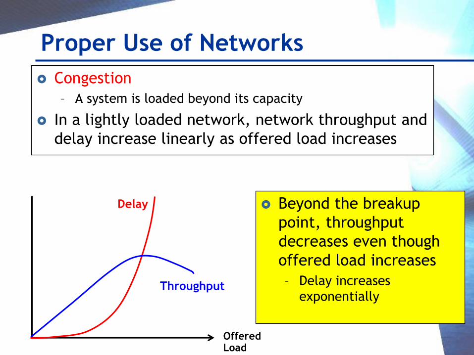
Proper Use of Networks
Congestion
– A system is loaded beyond its capacity
In a lightly loaded network, network throughput and
delay increase linearly as offered load increases
Beyond the breakup
point, throughput
decreases even though
offered load increases
– Delay increases
exponentially
OfferedLoad
Delay
Throughput

SNU SCONE lab. 3
Congestion Control & Resource
Allocation The only solution to the congestion problem is to
throttle the packets entered into the network
– Little’s theorem
Two ways to solve the congestion problem
– Congestion control
– Resource allocation
Congestion control
– Send packets, if congestion occurs reduce the sending rate
– Mostly performed at hosts
Resource allocation
– Request resources (e.g. bandwidth) before sending packets
– Limits the sending rate to the agreed amount
Congestion Avoidance
SNU SCONE lab.
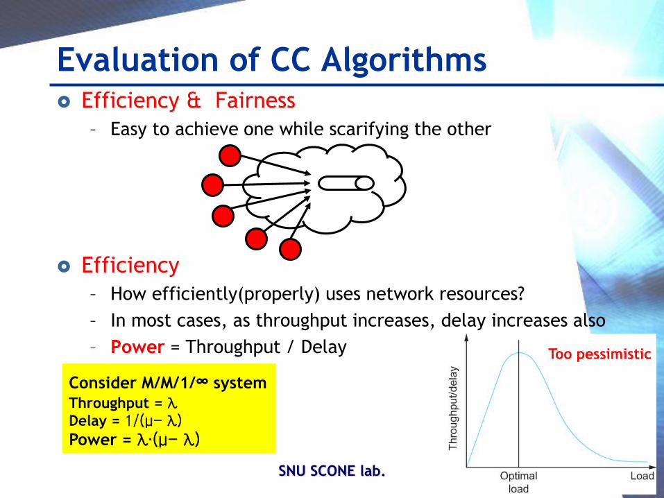
Evaluation of CC Algorithms Efficiency & Fairness
– Easy to achieve one while scarifying the other
Efficiency
– How efficiently(properly) uses network resources?
– In most cases, as throughput increases, delay increases also
– Power = Throughput / Delay
Consider M/M/1/∞ system
Throughput = λDelay = 1/(μ- λ)
Power = λ∙(μ- λ)
Too pessimistic
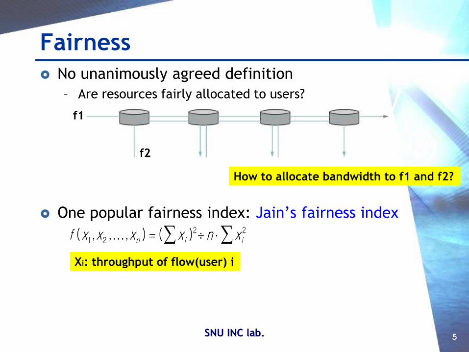
Fairness
No unanimously agreed definition
– Are resources fairly allocated to users?
One popular fairness index: Jain’s fairness index
SNU INC lab. 5
f x x x x n xn i i( , ,..., ) ( )1 22 2
f1
f2
How to allocate bandwidth to f1 and f2?
Xi: throughput of flow(user) i
6
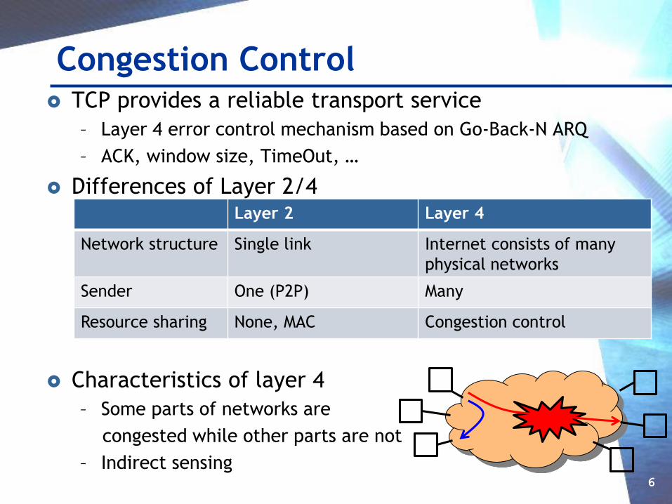
Congestion Control TCP provides a reliable transport service
– Layer 4 error control mechanism based on Go-Back-N ARQ
– ACK, window size, TimeOut, …
Differences of Layer 2/4
Characteristics of layer 4
– Some parts of networks are
congested while other parts are not
– Indirect sensing
Layer 2 Layer 4
Network structure Single link Internet consists of many
physical networks
Sender One (P2P) Many
Resource sharing None, MAC Congestion control
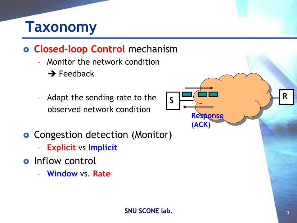
Taxonomy
Closed-loop Control mechanism
– Monitor the network condition
Feedback
– Adapt the sending rate to the
observed network condition
Congestion detection (Monitor)
– Explicit vs Implicit
Inflow control
– Window vs. Rate
SNU SCONE lab. 7
Response
(ACK)
SR
SNU SCONE lab. 8
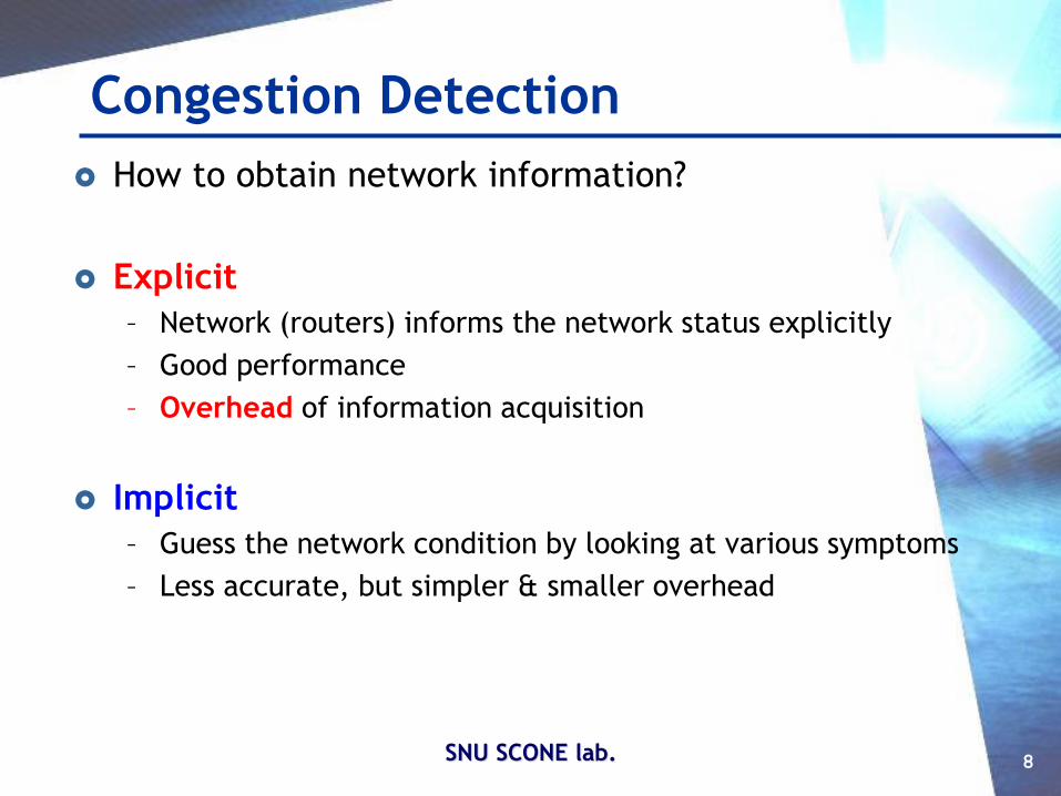
Congestion Detection
How to obtain network information?
Explicit
– Network (routers) informs the network status explicitly
– Good performance
– Overhead of information acquisition
Implicit
– Guess the network condition by looking at various symptoms
– Less accurate, but simpler & smaller overhead

9
Input Control - 1
How to regulate the packet inflow?
Window based– Like the ARQ window
• Limit the number of packets that can be sent without ACKs
– Vary window size according to the network conditions
Plusses for window– No need for fine-grained timer
– Self-limiting
Window size & Rate ?
S D
System
N=λ∙T
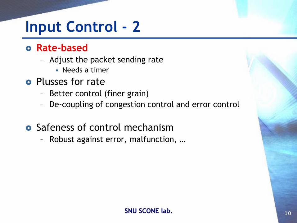
Input Control - 2
Rate-based– Adjust the packet sending rate
• Needs a timer
Plusses for rate– Better control (finer grain)
– De-coupling of congestion control and error control
Safeness of control mechanism– Robust against error, malfunction, …
SNU SCONE lab. 10

TCP Congestion Control
SNU SCONE lab. 12
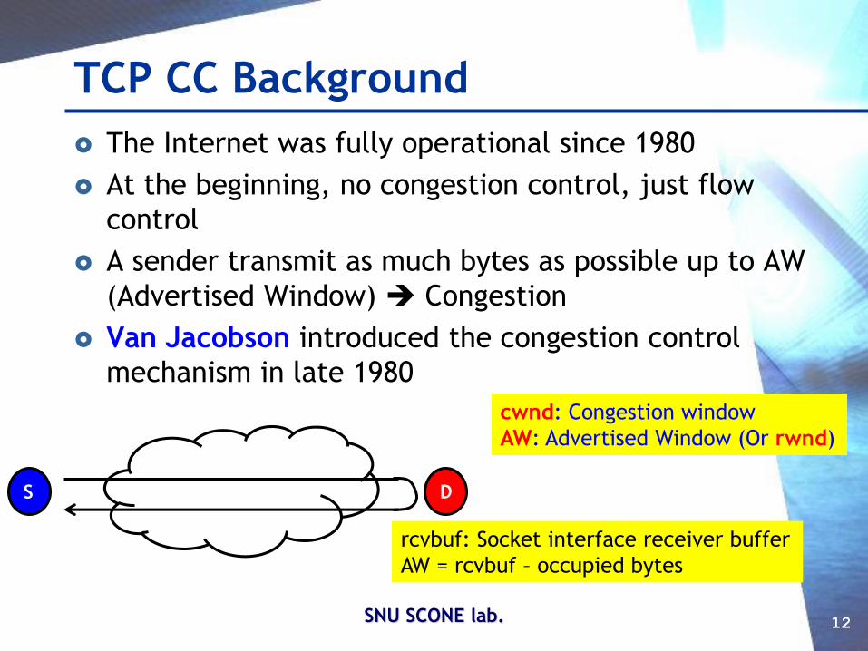
TCP CC Background
The Internet was fully operational since 1980
At the beginning, no congestion control, just flow
control
A sender transmit as much bytes as possible up to AW
(Advertised Window) Congestion
Van Jacobson introduced the congestion control
mechanism in late 1980
cwnd: Congestion window
AW: Advertised Window (Or rwnd)
S D
rcvbuf: Socket interface receiver buffer
AW = rcvbuf – occupied bytes

TCP CC & Error Control
TCP provides end-to-end reliable delivery service
– Go-back-N ARQ & optional Selective repeat
• Learn SACK (Selective ACK) option
For each segment, a receiver returns ACK to a sender• Learn delayed ACK option
Sender measures RTT Use it for setting TO value
SNU SCONE lab. 13
S R
DATA segment
ACK segment
Window size N ≡ Number of in-flight packets & ACKs
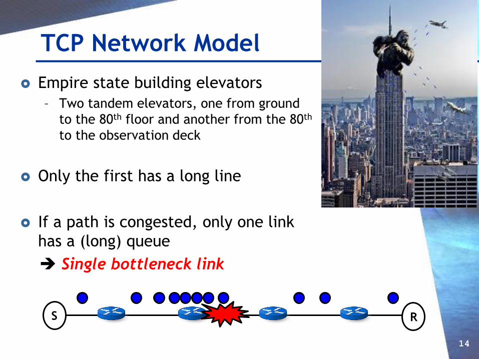
TCP Network Model
Empire state building elevators
– Two tandem elevators, one from ground
to the 80th floor and another from the 80th
to the observation deck
Only the first has a long line
If a path is congested, only one link
has a (long) queue
Single bottleneck link
14
S R

TCP Network Model - 2
Constant RTT
– RTTs are about the same whether the path is congested or not
– Routers have a (relatively) very small buffer (e.g. buffer size is
< 1000 packets)
– Link speed is ~1 Tbps
Queueing delay can be ignored for long distance paths
SNU SCONE lab. 15
Constant RTT assumption is not valid anymore
Buffer bloat problem
N=λ∙T
16
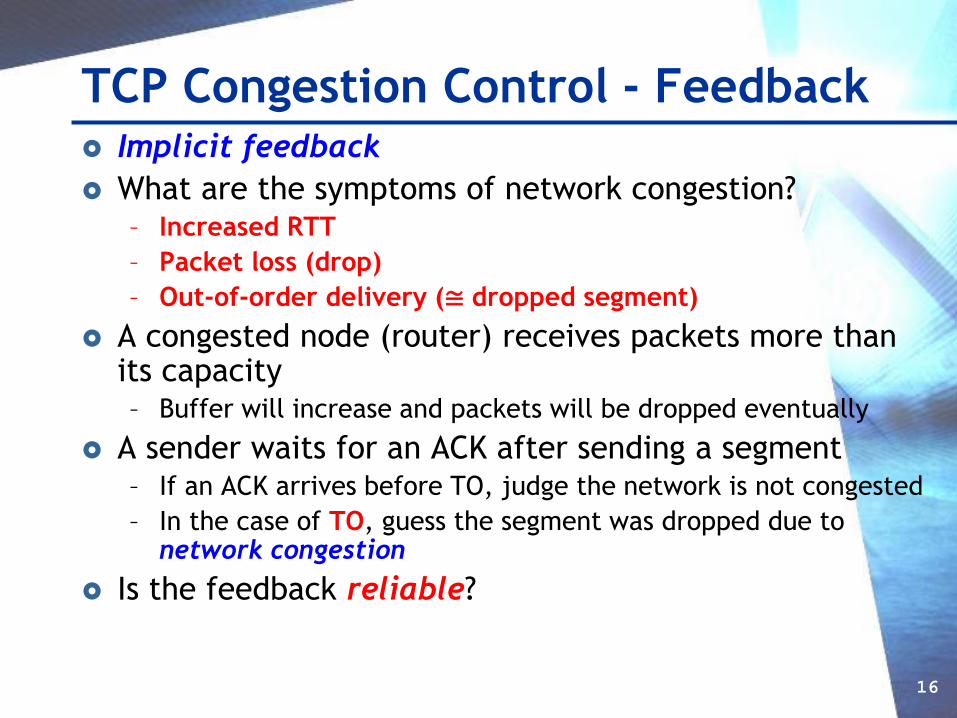
TCP Congestion Control - Feedback Implicit feedback
What are the symptoms of network congestion?– Increased RTT
– Packet loss (drop)
– Out-of-order delivery (≅ dropped segment)
A congested node (router) receives packets more than its capacity– Buffer will increase and packets will be dropped eventually
A sender waits for an ACK after sending a segment– If an ACK arrives before TO, judge the network is not congested
– In the case of TO, guess the segment was dropped due to network congestion
Is the feedback reliable?

SNU SCONE lab.
TCP Congestion Control - AIMD
Additive Increase (AI)– All ACKs arrive before TO Not congested
– Increase window size (cwnd, N) by one MSS (Max. Segment Size) at each RTT
– Increment rule
• inc = MSS * (MSS / cwnd)
• cwnd += inc
Multiplicative Decrease (MD)– TO Congested
– Decrease cwnd in the case of TO
– cwnd = cwnd / 2
– TCP may drop cwnd to 1 MSS
Note: cwnd unit is byte
SNU SCONE lab. 18
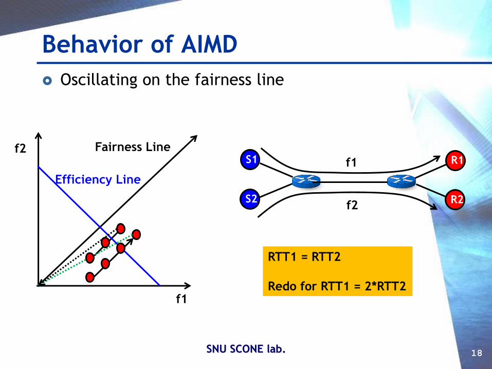
Behavior of AIMD
Oscillating on the fairness line
Fairness Line
Efficiency Line
f1
f2S1
S2
R1
R2
f1
f2
RTT1 = RTT2
Redo for RTT1 = 2*RTT2
19
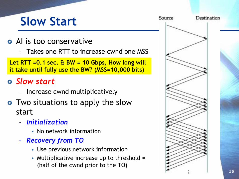
Slow Start
AI is too conservative
– Takes one RTT to increase cwnd one MSS
Slow start
– Increase cwnd multiplicatively
Two situations to apply the slow
start
– Initialization
• No network information
– Recovery from TO
• Use previous network information
• Multiplicative increase up to threshold =
(half of the cwnd prior to the TO)
Let RTT =0.1 sec. & BW = 10 Gbps, How long will
it take until fully use the BW? (MSS=10,000 bits)
SNU INC lab. 20
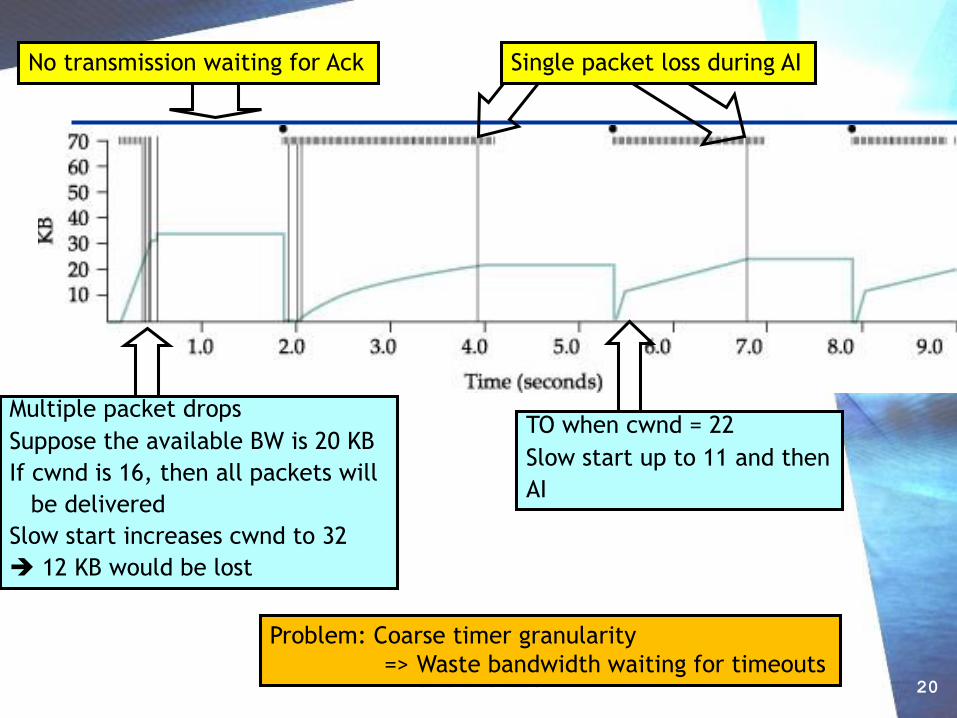
Example Trace
Problem: Coarse timer granularity
=> Waste bandwidth waiting for timeouts
Multiple packet drops
Suppose the available BW is 20 KB
If cwnd is 16, then all packets will
be delivered
Slow start increases cwnd to 32
12 KB would be lost
No transmission waiting for Ack
TO when cwnd = 22
Slow start up to 11 and then
AI
Single packet loss during AI
SNU SCONE lab. 21
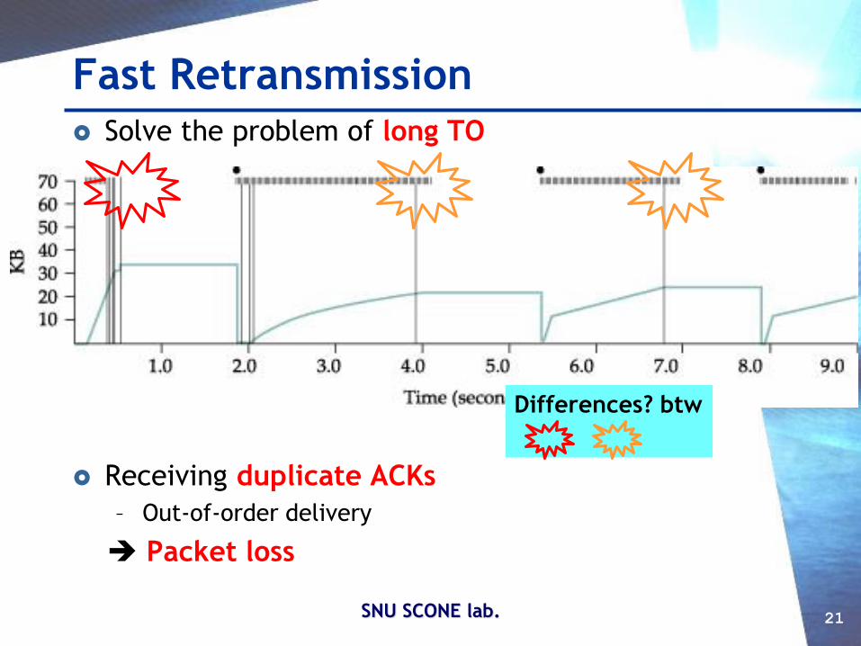
Fast Retransmission
Solve the problem of long TO
Receiving duplicate ACKs
– Out-of-order delivery
Packet loss
Differences? btw
SNU SCONE lab. 22
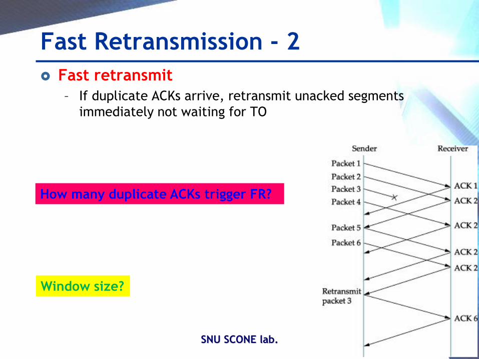
Fast Retransmission - 2
Fast retransmit
– If duplicate ACKs arrive, retransmit unacked segments
immediately not waiting for TO
How many duplicate ACKs trigger FR?
Window size?
23
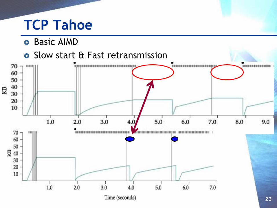
TCP Tahoe Basic AIMD
Slow start & Fast retransmission

SNU SCONE lab. 24
Fast Recovery & TCP Reno
Mechanism
– Remove the slow start phase in the case of Fast Retransmit
– Go directly to half the last CW
– Increase cwnd additively from the threshold
TCP Reno
– In addition to TCP Tahoe, add fast recovery and (header
prediction + delayed ACK) mechanisms
What is Header Prediction?
Learn CUBIC, BIC by Injong Rhee
Congestion Avoidance
Protocols

SNU SCONE lab. 26
Congestion Avoidance
Prevent congestion
Detect the symptoms when congestion may occur soon
and adjust the sending rate
Many methods rely on (explicit) feedbacks from
routers
Resource
Allocation
Congestion
Control
Congestion
Avoidance
SNU SCONE lab. 27
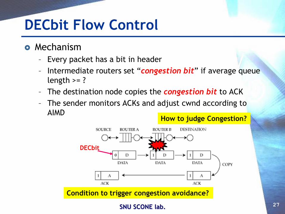
DECbit Flow Control
Mechanism
– Every packet has a bit in header
– Intermediate routers set “congestion bit” if average queue
length >= ?
– The destination node copies the congestion bit to ACK
– The sender monitors ACKs and adjust cwnd according to
AIMD
DECbit
How to judge Congestion?
Condition to trigger congestion avoidance?
SNU SCONE lab. 28
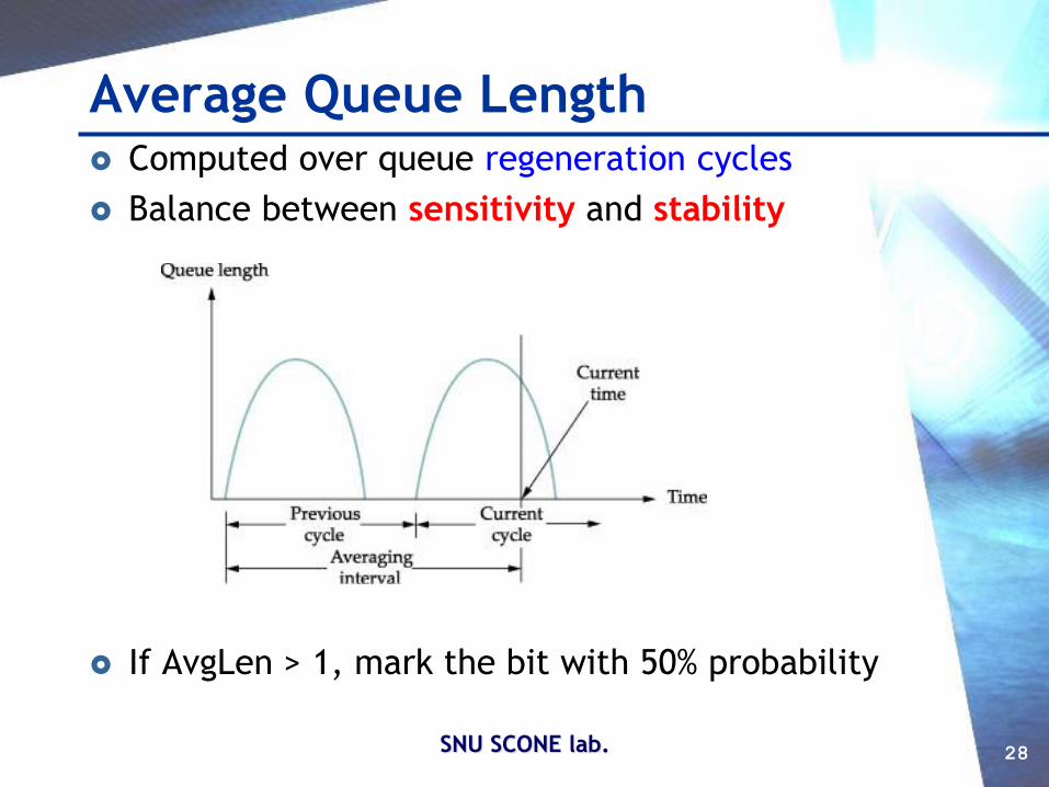
Average Queue Length Computed over queue regeneration cycles
Balance between sensitivity and stability
If AvgLen > 1, mark the bit with 50% probability
SNU SCONE lab. 29
Source Actions
Observe bits over past + present window size
– Should not take control actions too fast!
– Wait for past change to take effect
If more than 50% set, then decrease window, else
increase
Additive increase, multiplicative decrease
– cwnd = cwnd + 1
– cwnd = 0.875 * cwnd
SNU SCONE lab. 30
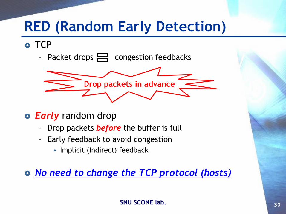
RED (Random Early Detection) TCP
– Packet drops congestion feedbacks
Early random drop
– Drop packets before the buffer is full
– Early feedback to avoid congestion
• Implicit (Indirect) feedback
No need to change the TCP protocol (hosts)
Drop packets in advance
31
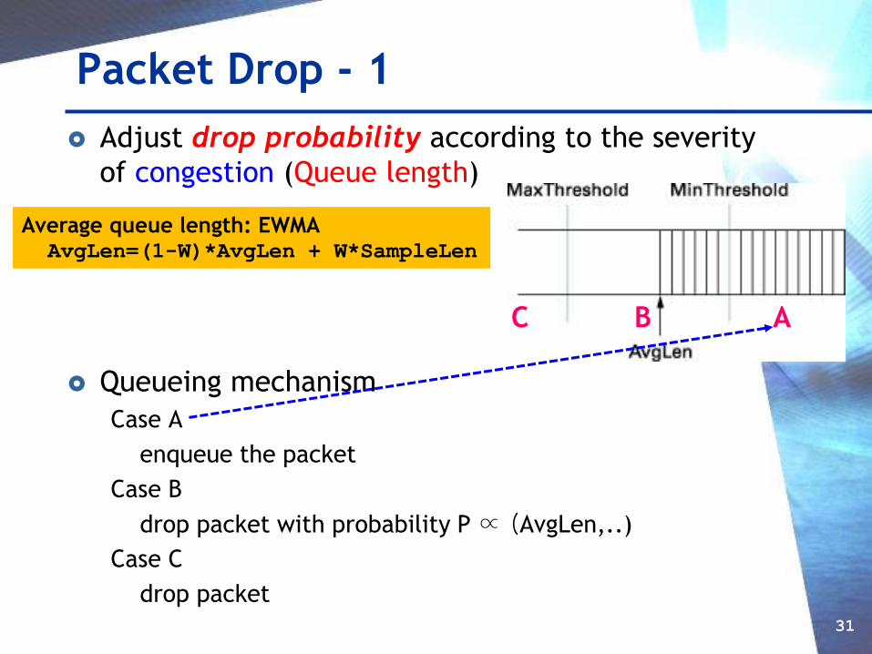
Packet Drop - 1
Adjust drop probability according to the severity
of congestion (Queue length)
Queueing mechanism
Case A
enqueue the packet
Case B
drop packet with probability P ∝ (AvgLen,..)
Case C
drop packet
C B A
Average queue length: EWMAAvgLen=(1-W)*AvgLen + W*SampleLen

SNU SCONE lab. 32
TCP Vegas
Congestion
Queued packets increases
– How to estimate the number of packets queued inside
the network?
Idea: symptoms that congestion will happen soon
– RTT is growing (Note: Constant RTT assumption)
– Sending rate flattens
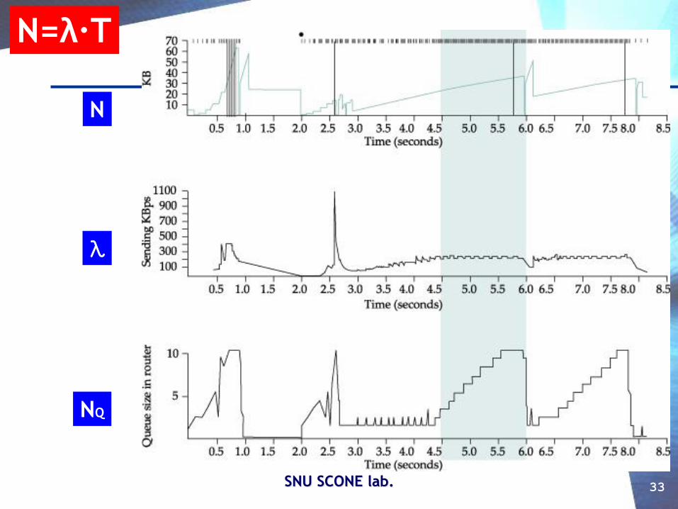
SNU SCONE lab. 33
N
λ
NQ
N=λ∙T

SNU SCONE lab. 34
TCP Vegas
Number of packets (bytes) in the network (= cwnd)
= In-transit packets (Ns) + Queued packets (NQ)
Time in the system (= RTT)
= In-transit time + Queueing time
In-transit time = the RTT when there is no queueing– BaseRTT
– Approximate it w/ the Minimum RTT that’s been observed
S R
Estimate the # of packets
in the queue
We know them
What other values can we know(estimate)?
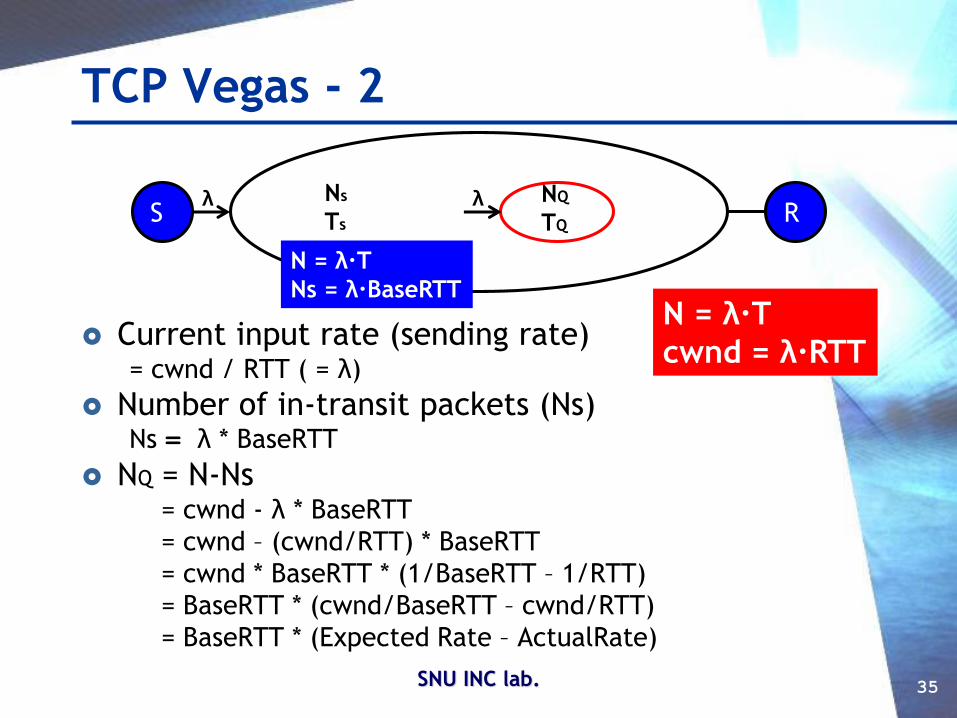
TCP Vegas - 2
Current input rate (sending rate)= cwnd / RTT ( = λ)
Number of in-transit packets (Ns) Ns = λ * BaseRTT
NQ = N-Ns= cwnd - λ * BaseRTT
= cwnd – (cwnd/RTT) * BaseRTT
= cwnd * BaseRTT * (1/BaseRTT – 1/RTT)
= BaseRTT * (cwnd/BaseRTT – cwnd/RTT)
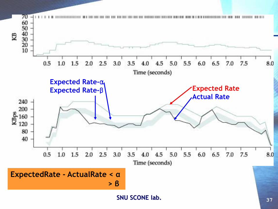
= BaseRTT * (Expected Rate – ActualRate)
SNU INC lab. 35
S Rλ λNs
Ts
NQ
TQ
N = λ∙T
cwnd = λ∙RTT
N = λ∙T
Ns = λ∙BaseRTT
SNU SCONE lab. 36
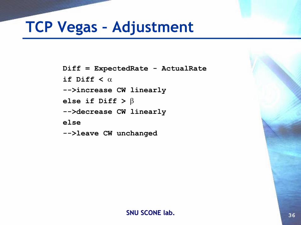
TCP Vegas – Adjustment
Diff = ExpectedRate - ActualRate
if Diff <
-->increase CW linearly
else if Diff >
-->decrease CW linearly
else
-->leave CW unchanged
SNU SCONE lab. 37
Expected Rate
Actual Rate
Expected Rate-αExpected Rate-β
ExpectedRate - ActualRate < α
> β
SNU SCONE lab. 38
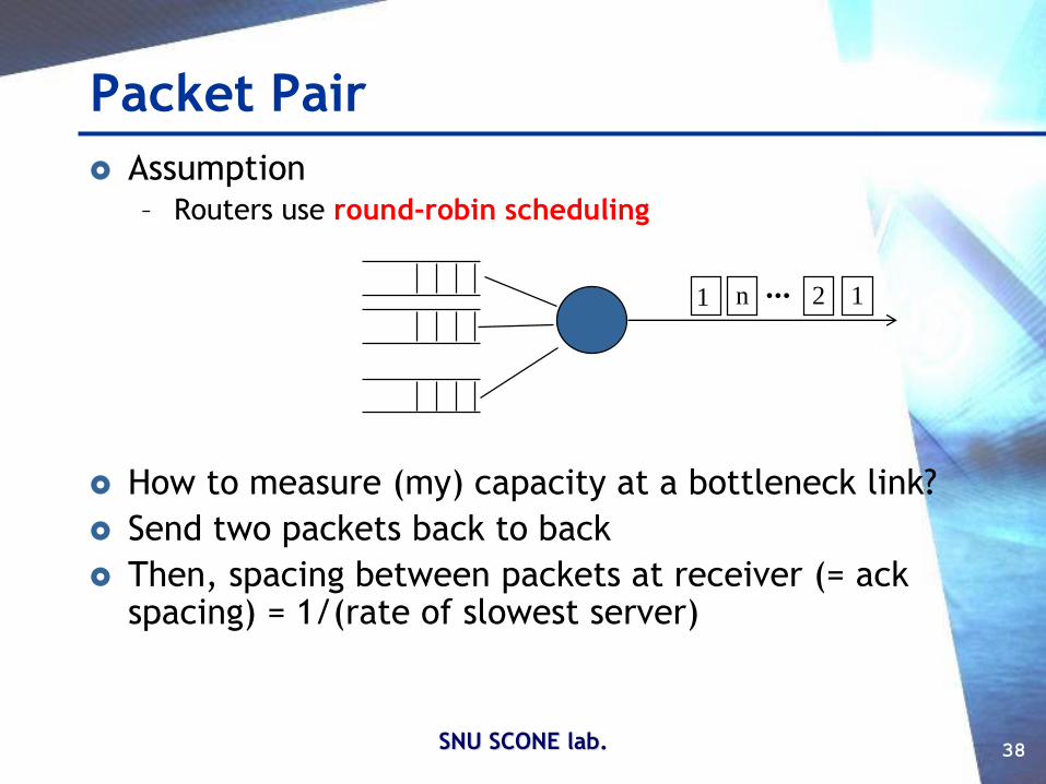
Packet Pair
Assumption– Routers use round-robin scheduling
How to measure (my) capacity at a bottleneck link?
Send two packets back to back
Then, spacing between packets at receiver (= ackspacing) = 1/(rate of slowest server)
1n 21 …
SNU SCONE lab. 39
Packet Pair
SNU SCONE lab. 40
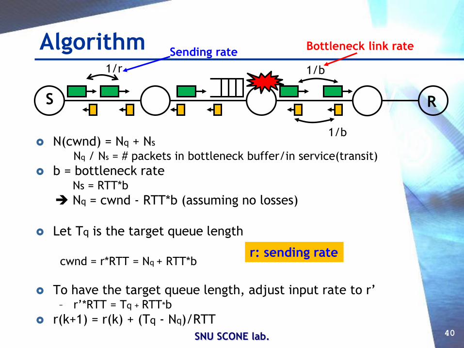
Algorithm
N(cwnd) = Nq + Ns
Nq / Ns = # packets in bottleneck buffer/in service(transit)
b = bottleneck rateNs = RTT*b
Nq = cwnd - RTT*b (assuming no losses)
Let Tq is the target queue length
cwnd = r*RTT = Nq + RTT*b
To have the target queue length, adjust input rate to r’– r’*RTT = Tq + RTT*b
r(k+1) = r(k) + (Tq - Nq)/RTT
S R
1/b
1/b
Bottleneck link rate
1/r
Sending rate
r: sending rate

Resource Allocation
QoS(Quality of Service)

SNU SCONE lab. 42
QoS (Quality of Service)
Real-time service
– Service that requires strict delay and loss performance
– Ex: A voice call requires the delay of less than 200-300 ms
Performance aspects
– Delay
– Loss
– Jitter
– Bandwidth
SNU SCONE lab. 43
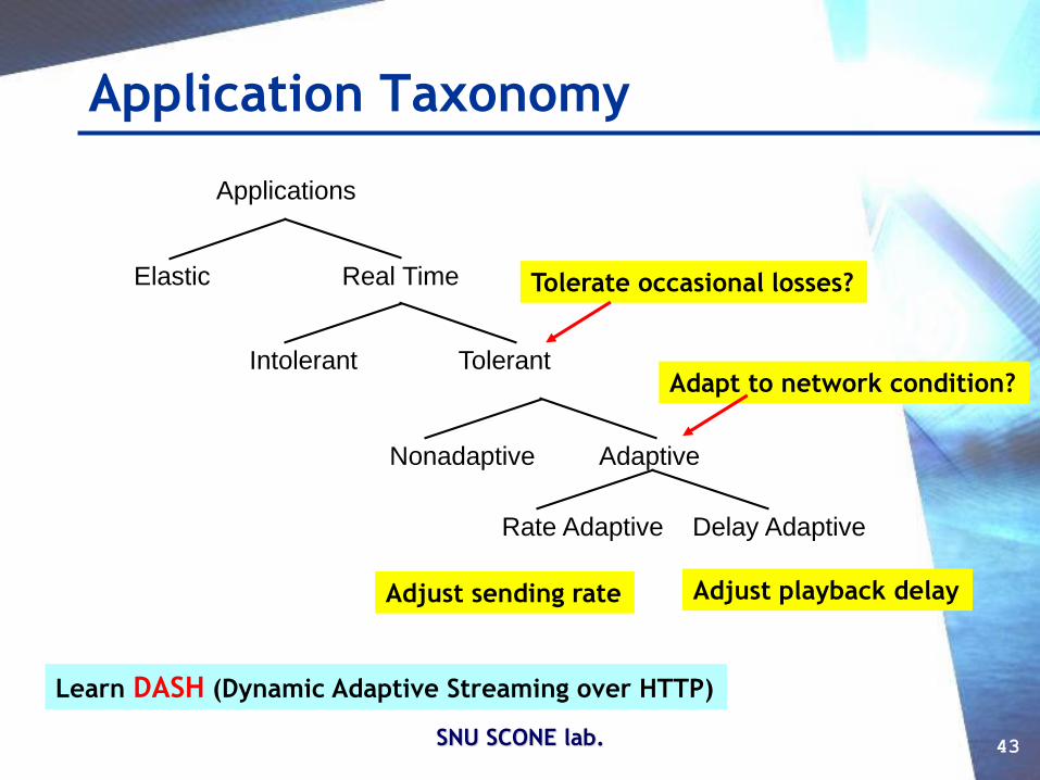
Application Taxonomy
Applications
Elastic Real Time
Intolerant Tolerant
Nonadaptive Adaptive
Rate Adaptive Delay Adaptive
Tolerate occasional losses?
Adapt to network condition?
Adjust playback delayAdjust sending rate
Learn DASH (Dynamic Adaptive Streaming over HTTP)
SNU SCONE lab. 44
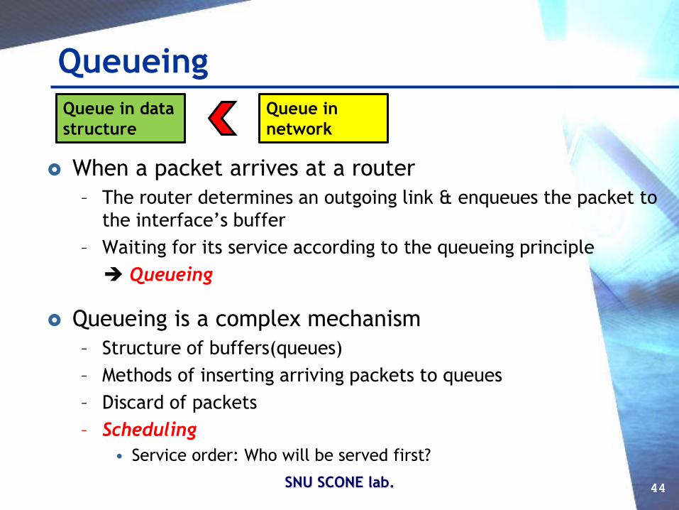
Queueing
When a packet arrives at a router
– The router determines an outgoing link & enqueues the packet to
the interface’s buffer
– Waiting for its service according to the queueing principle
Queueing
Queueing is a complex mechanism
– Structure of buffers(queues)
– Methods of inserting arriving packets to queues
– Discard of packets
– Scheduling
• Service order: Who will be served first?
Queue in data
structure
Queue in
network
SNU SCONE lab. 45
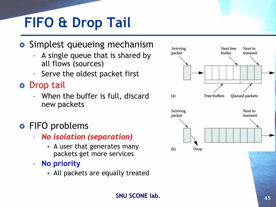
FIFO & Drop Tail
Simplest queueing mechanism– A single queue that is shared by
all flows (sources)
– Serve the oldest packet first
Drop tail– When the buffer is full, discard
new packets
FIFO problems– No isolation (separation)
• A user that generates many packets get more services
– No priority
• All packets are equally treated

46
Multiple Queues Isolation
Multiple queues each dedicated to– Priority
– Flow
A packet is inserted to the queue of its priority/flow
Insertion & dropping to/from each queue may be same as a single queue
Scheduling– Priority scheduling
• Serve all high priority packets before serving low priority packets
– Fair scheduling
• Serve packets fairly (equally)
What is a flow?
?
47
RR (Round Robin) Fair service
– Allocate resources equally to all customers
Round Robin (RR)– Serve each queue once per round
What is the service (scheduling) unit?
Packet by packet RR– Send one packet from each flow per round
– Unfair if packet sizes are different
Bit by bit RR– Send one bit from each flow per round
– Fair but Impossible
How to emulate bit by bit RR?
SNU SCONE lab. 48
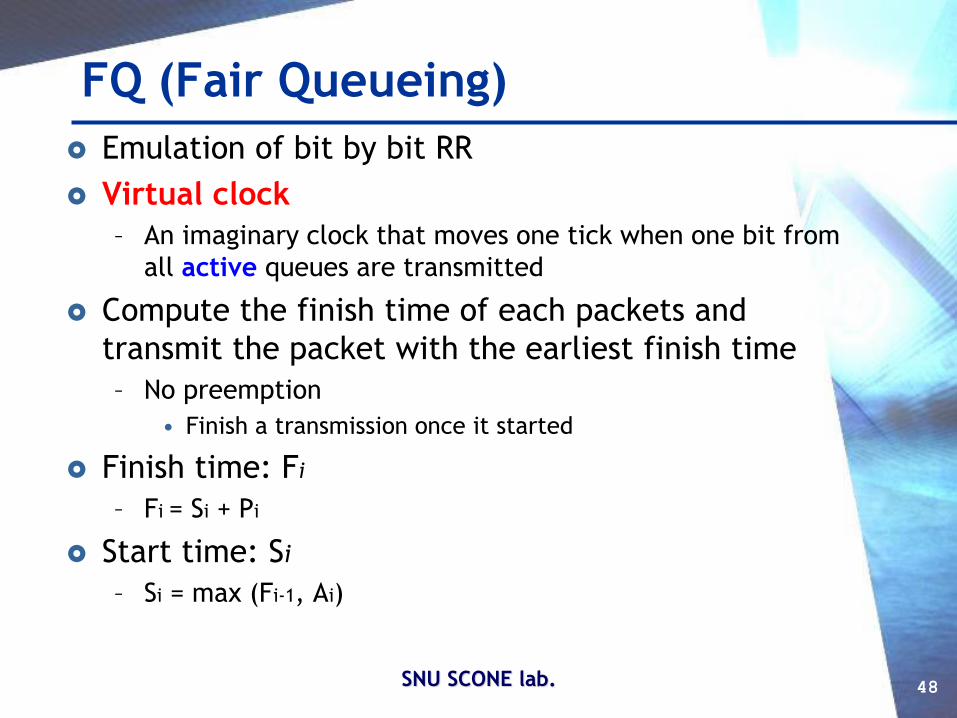
FQ (Fair Queueing)
Emulation of bit by bit RR
Virtual clock
– An imaginary clock that moves one tick when one bit from
all active queues are transmitted
Compute the finish time of each packets and
transmit the packet with the earliest finish time
– No preemption
• Finish a transmission once it started
Finish time: Fi
– Fi = Si + Pi
Start time: Si
– Si = max (Fi-1, Ai)
49
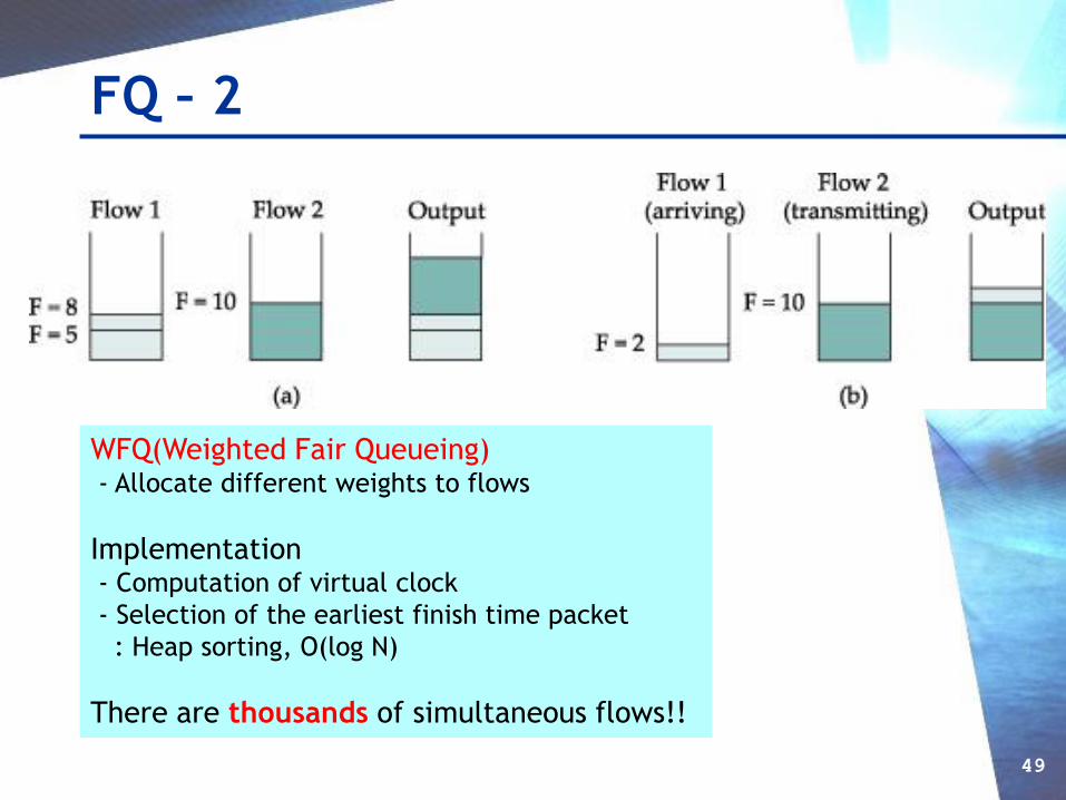
FQ – 2
WFQ(Weighted Fair Queueing)- Allocate different weights to flows
Implementation- Computation of virtual clock
- Selection of the earliest finish time packet
: Heap sorting, O(log N)
There are thousands of simultaneous flows!!
SNU SCONE lab. 50
QoS Support Architectures Mechanisms to support QoS
– Separation (Classification)
– Different treatment (Scheduling)
– Resource reservation
Blocking (admission control) & Regulation (Policing)
Two QoS support approaches
IntServ (Integrated Service) architecture
– Fine-grained, Reserve resources for each flow
– Strict QoS support
DiffServ (Differentiated Service) architecture
– Coarse-grained, Group flows into a priority class
– Scalability
SNU SCONE lab. 51
IntServ Classify traffic into three categories
– GS (Guaranteed Service)
• Strict support of QoS requirements
• e.g. VoIP
– CS (Controlled-load Service)
• Performance of lightly loaded network
• e.g. Streaming
– BS (Best-effort Service)
Mechanisms
– Admission control & Reservation
– Classification
– Scheduling
– Policing (Regulation)
SNU SCONE lab. 52
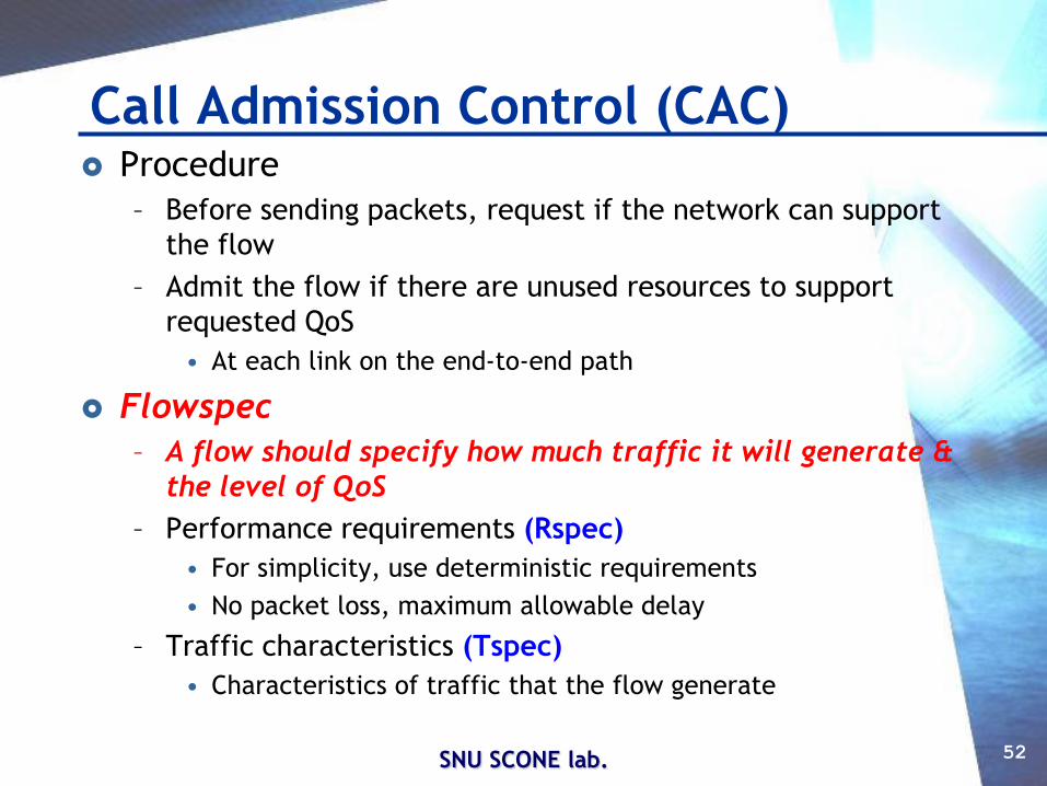
Call Admission Control (CAC) Procedure
– Before sending packets, request if the network can support
the flow
– Admit the flow if there are unused resources to support
requested QoS
• At each link on the end-to-end path
Flowspec
– A flow should specify how much traffic it will generate &
the level of QoS
– Performance requirements (Rspec)
• For simplicity, use deterministic requirements
• No packet loss, maximum allowable delay
– Traffic characteristics (Tspec)
• Characteristics of traffic that the flow generate
SNU SCONE lab. 53
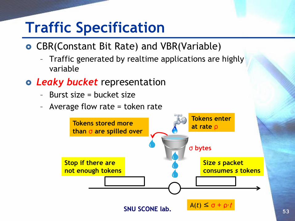
Traffic Specification CBR(Constant Bit Rate) and VBR(Variable)
– Traffic generated by realtime applications are highly
variable
Leaky bucket representation
– Burst size = bucket size
– Average flow rate = token rate
σ bytes
Tokens enter
at rate ρ
Stop if there are
not enough tokens
Size s packet
consumes s tokens
Tokens stored more
than σ are spilled over
A(t) ≤ σ + ρ∙t

SNU SCONE lab. 54
Parekh-Gallager Theorem
How to satisfy the strictest QoS requirement?
Worst-case end-to-end delay (no packet loss)– Assume that bw are allocated to a flow at each WFQ scheduler along
its path, so that the least bw it is allocated is g
– Let it be leaky-bucket regulated such that # bits sent in time [t1, t2] <=
ρ(t2 - t1) +
– Let the connection pass through K routers(schedulers), where the k-th
scheduler has a rate r(k)
– Let the largest packet size in the network be P
1
1 1
)(///___K
k
K
k
krPgPgdelayendtoend
SNU SCONE lab. 55
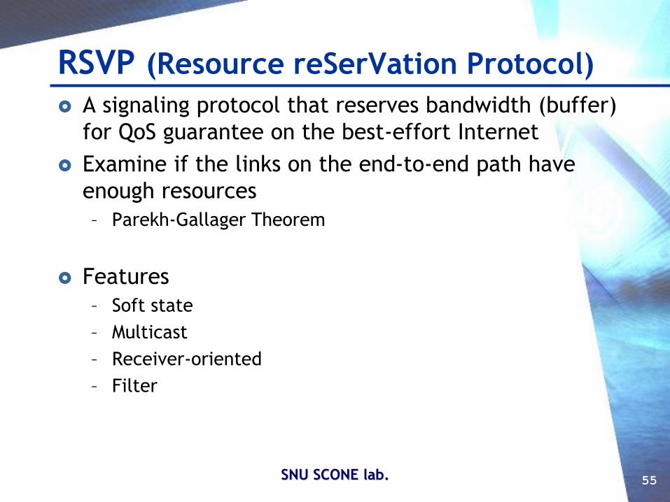
RSVP (Resource reSerVation Protocol)
A signaling protocol that reserves bandwidth (buffer)
for QoS guarantee on the best-effort Internet
Examine if the links on the end-to-end path have
enough resources
– Parekh-Gallager Theorem
Features
– Soft state
– Multicast
– Receiver-oriented
– Filter
SNU SCONE lab. 56
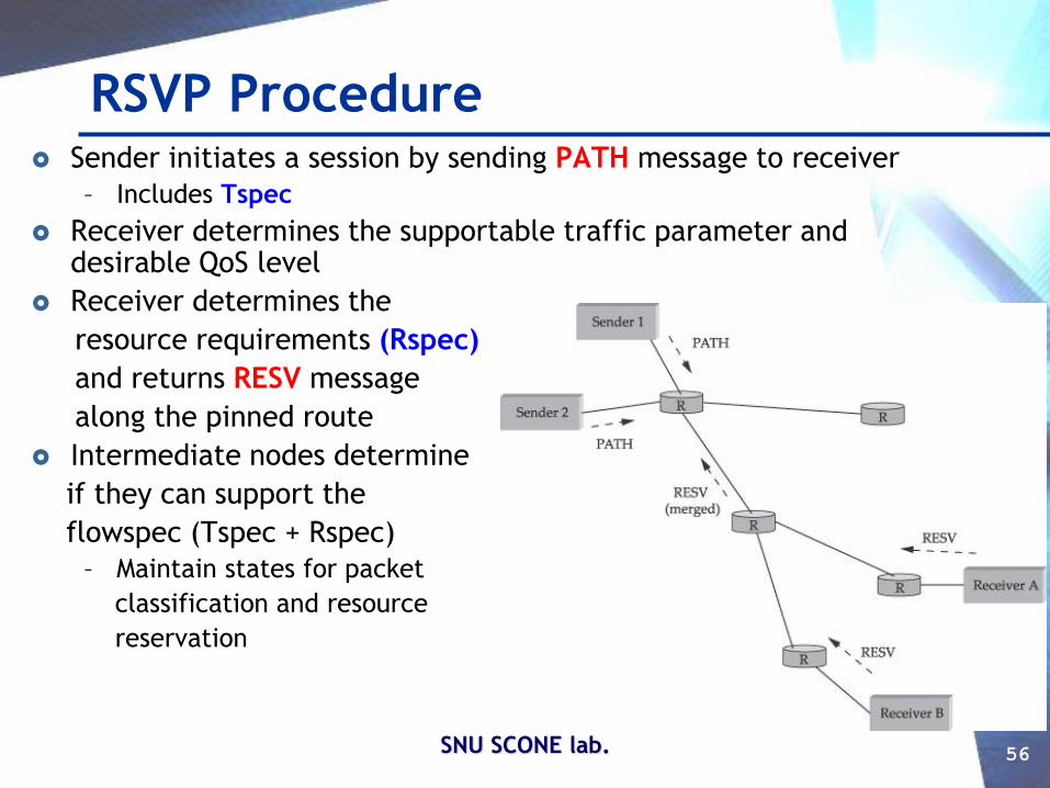
RSVP Procedure Sender initiates a session by sending PATH message to receiver
– Includes Tspec
Receiver determines the supportable traffic parameter and desirable QoS level
Receiver determines the
resource requirements (Rspec)
and returns RESV message
along the pinned route
Intermediate nodes determine
if they can support the
flowspec (Tspec + Rspec)
– Maintain states for packet
classification and resource
reservation
SNU SCONE lab. 57
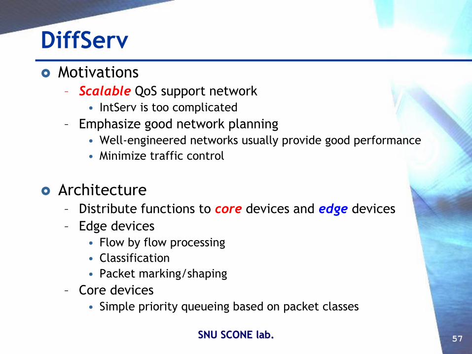
DiffServ
Motivations– Scalable QoS support network
• IntServ is too complicated
– Emphasize good network planning
• Well-engineered networks usually provide good performance
• Minimize traffic control
Architecture– Distribute functions to core devices and edge devices
– Edge devices
• Flow by flow processing
• Classification
• Packet marking/shaping
– Core devices
• Simple priority queueing based on packet classes
SNU SCONE lab. 58
DiffServ
Service classes
– EF (Expedited Forwarding)
• Transmit the packet before any other packets
– AF (Assured Forwarding)
• Usually receive good performance
– BF
Mechanisms
– Admission control
• For EF and AF services
– Regulator
• EF
– Marker
• AF
SNU SCONE lab. 59
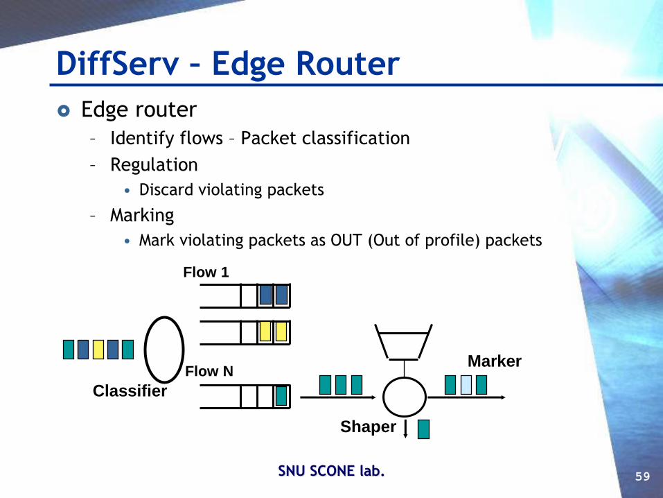
DiffServ – Edge Router
Edge router
– Identify flows – Packet classification
– Regulation
• Discard violating packets
– Marking
• Mark violating packets as OUT (Out of profile) packets
Classifier
Flow 1
Flow N
Shaper
Marker
SNU SCONE lab. 60
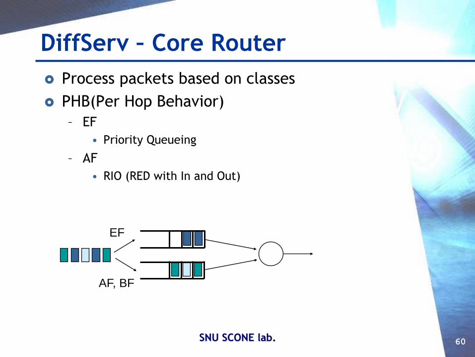
DiffServ – Core Router
Process packets based on classes
PHB(Per Hop Behavior)
– EF
• Priority Queueing
– AF
• RIO (RED with In and Out)
EF
AF, BF
SNU SCONE lab. 61
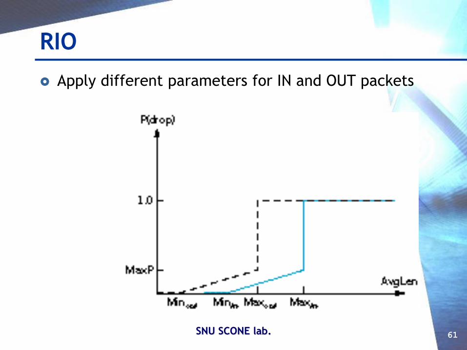
RIO
Apply different parameters for IN and OUT packets
Recommended