Dynamic Resource Allocation in Disaster Response ...web.physics.ucsb.edu/~complex/pubs/Dynamic Resource Allocation … · Dynamic Resource Allocation in Disaster Response: Tradeoffs

Dynamic Resource Allocation in Disaster Response:Tradeoffs in Wildfire SuppressionNada Petrovic1*, David L. Alderson2, Jean M. Carlson3

1Center for Research on Environmental Decisions, Columbia University, New York, New York, United States of America, 2Operations Research Department, Naval

Postgraduate School, Monterey, California, United States of America, 3 Physics Department, University of California, Santa Barbara, Santa Barbara, California, United States

of America

Abstract

Challenges associated with the allocation of limited resources to mitigate the impact of natural disasters inspirefundamentally new theoretical questions for dynamic decision making in coupled human and natural systems. Wildfires areone of several types of disaster phenomena, including oil spills and disease epidemics, where (1) the disaster evolves on thesame timescale as the response effort, and (2) delays in response can lead to increased disaster severity and thus greaterdemand for resources. We introduce a minimal stochastic process to represent wildfire progression that nonethelessaccurately captures the heavy tailed statistical distribution of fire sizes observed in nature. We then couple this model for firespread to a series of response models that isolate fundamental tradeoffs both in the strength and timing of response andalso in division of limited resources across multiple competing suppression efforts. Using this framework, we computeoptimal strategies for decision making scenarios that arise in fire response policy.

Citation: Petrovic N, Alderson DL, Carlson JM (2012) Dynamic Resource Allocation in Disaster Response: Tradeoffs in Wildfire Suppression. PLoS ONE 7(4): e33285.doi:10.1371/journal.pone.0033285

Editor: Renaud Lambiotte, University of Namur, Belgium

Received August 19, 2011; Accepted February 12, 2012; Published April 13, 2012

Copyright: � 2012 Petrovic et al. This is an open-access article distributed under the terms of the Creative Commons Attribution License, which permitsunrestricted use, distribution, and reproduction in any medium, provided the original author and source are credited.

Funding: This work was supported by Office of Naval Research MURI grants N000140810747 (http://www07.grants.gov/search/search.do?oppId = 42747&mode= VIEW) and 0001408WR20242, the Bell Labs Graduate Research Fellowship, and the David and Lucile Packard Foundation (http://www.packard.org/). The funders had no role in study design, data collection and analysis, decision to publish, or preparation of the manuscript.

Competing Interests: The authors have declared that no competing interests exist.

* E-mail: [email protected]

Introduction

Wildfire progression is driven by inherently complex, inter-

connected, physical processes, involving a variety of factors,

including weather, vegetation, and terrain [1–4]. Wildfires are

difficult to predict in space and time, and thus it is hard to make

informed decisions about mitigation efforts, particularly the

allocation of limited resources during dynamic response. Further-

more, the areas and damages of wildfires both exhibit high

variability, heavy tailed statistics [5], implying that overall impacts

are dominated not by the typical, median size events, but rather by

the relatively rare, large events. This highlights the fundamental

importance of understanding tradeoffs between strength and

timing in mitigation efforts that may help prevent future wildfires

from growing out of control.

In recent years, wildfires in the United States have received

media attention due to rising suppression costs [6], which have

regularly exceeded expenditures of a billion dollars per year in the

new millennium [7]. A variety of potential driving factors have

been suggested [8], including a climate-driven increase in wildfire

activity [9–11], and development at the wildland urban interface

[12,13]. A cohesive strategy that takes into account both the

natural occurrence of wildfire on the landscape and its impact on

human lives is needed to determine the best course of action for

reducing these costs. The Federal Land Assistance, Management

and Enhancement Act (FLAME Act) of 2010 directs the U.S.

Department of Agriculture, the U.S. Department of the Interior,

and the U.S. Department of Homeland Security to develop

a Cohesive Wildfire Management Strategy to identify, among

other things, the most cost effective means for allocating fire

management budget resources. Thus, there is a need to un-

derstand not only the dynamics underlying wildfire behavior but

also how to allocate limited resources to mitigate fire damage.

In this paper we introduce a minimal model of wildfire

dynamics using the formalism of stochastic processes and queueing

theory. We divide the burnable substrate, which may be forest,

shrubland, or grassland depending on the region, into discrete

parcels that arrive in a queue when they begin to burn. The

growth rate of the number of parcels in the queue scales with the

current size of the queue, capturing the escalating dynamics

familiar in wildfire spread. Parcels exit the queue when they are

extinguished either by natural causes or human suppression. This

model reproduces the observed statistical distribution of wildfire

sizes, and it enables investigation of tradeoffs in suppression efforts

that are fundamental to decision making.

Our model is sufficiently general that it may apply to other

scenarios involving coupled dynamics of a disaster and response.

In the context of wildfires, our study is intended to be an

intermediate step between models with static fires [14,15] and

models with a detailed fire spread simulation [16,17]. It is not

intended to replace high fidelity simulations but will be used to

examine basic relationships, which can then be further explored

and verified with more realistic models. We comment on this in

more detail in the Discussion.

We focus specifically on time dynamics. However, spatial factors

such as prepositioning of resources are still implicitly included

through the time delay of resource arrival. Tradeoffs in strength

and timing are particularly relevant when considering resource

PLoS ONE | www.plosone.org 1 April 2012 | Volume 7 | Issue 4 | e33285

allocations to simultaneously occurring fires, which may be

evolving on different time scales.

Our Contributions in ContextThere are many research efforts that are complementary to

ours, having focused primarily on spatial rather than temporal

aspects of the problem. A rich literature exists within operations

research, focusing on optimization of wildfire response [18],

including models with realistic fire spread and various types of

suppression resources [16,17,19]. Because of the computational

complexity inherent in simulating a single fire, much less multiple

co-occurring fires or a statistical distribution of fires over time,

these models often abstract away the time dynamics of individual

fires. In many existing studies, the decision variable relates to

spatial prepositioning of resources for the initial response.

However, because wildfires are fundamentally both geospatial

and dynamic, decision making tools must ultimately capture both

the spatio-temporal spread of the fire itself and the geographic

locations and transportation of suppression resources.

One aspect of wildfires that has received considerable attention

in the complex systems literature is the power law distribution of

fire sizes: P(F )*F{a where F is the footprint (i.e., total burn area)

of the fire and P(F) is the probability of a fire being larger than or

equal to size F. Fires are not unique in this regard; many disparate

disaster phenomena exhibit power law statistics when losses are

tallied [20,21], and many biological, technological, and social

systems also exhibit power laws [22–24]. Although these

observations have led to widespread association of power law

statistics with a key signature of self-organization in complex

systems [25,26], there are mathematical, statistical, and data-

analytic arguments that suggest power law distributions should be

the natural null hypothesis for high variability phenomena [27].

Power law statistics are by no means unique or unexpected for

wildfires. However, the impact of power law distributions for

policy and decision making has not been investigated in much

detail, yet is critically important, especially in the case of natural

disasters. This heavy tailed statistical form is intrinsically linked

with uncertainty and high variability in observations: most fires are

small, while most of the area burned is contained in the few largest

events. In fact, in the context of wildfires, it has been noted that the

top 1% of large fires burn 80–96% of the total area [28]. Another

consequence of this mathematical form is that a large event, many

times bigger than anything seen recently, is not only possible but is

also consistent with the distribution. This is particularly significant

when planning for a worst case scenario.

Although power law statistics are observed in many systems,

a particularly interesting feature is that the exponent for wildfires,

a, clusters around 1/2 for data sets spanning a wide range of

geographic regions and time frames [4]. In general, different

disaster types (e.g., fires, hurricanes, earthquakes) exhibit varying

values of the exponent, suggesting that the relative scaling of

physical processes, tradeoffs, and constraints may be different in

each case [29–31]. The consistent value of the exponent a for

wildfire distributions, despite varying vegetation, weather, and

terrain, suggests that there may be a common mechanism that

drives wildfires across a wide range of fire regimes.

Several mechanisms for power laws have been discussed in the

context of wildfires, and simple models have been introduced to

illustrate these mechanisms. One example is Self Organized

Criticality (SOC) [32,33], which aims to explain the presence of

power laws as the consequence of a dynamical system operating at

a critical phase transition. Sandpile cellular automata are the

canonical example of SOC [25], combining an infinitesimal rate

for discrete and spatially random reloading of the system with

a threshold rule for event propagation, resulting in power law

distributions. Extrapolation of this basic mechanism of slow,

random regrowth with fast event propagation, terminating at grid

locations where the threshold criterion for propagation is not met,

has made SOC a popular topic within the complex systems

community.

The phase transition underlying the SOC forest fire model is

a percolation transition, associated with a critical density at which

nearest neighbor connectivity first extends from one side of

a discrete lattice to another. The percolation transition is

fundamentally statistical, describing the average behavior of an

ensemble consisting of all possible configurations of occupied (by

fuel) and vacant (no fuel) sites, characterized only by the fuel

density. Percolation is the most widely studied model of criticality

in statistical and mathematical physics because it is so simple,

enabling rigorous analysis and large scale simulations [34]. In the

context of wildfires, the SOC model can be loosely interpreted as

a fuel driven model, because fire propagates through connected

clusters of fuel occupied sites, terminating only at vacancies.

However, even in a physical model of fuel driven wildfires, the

biology, ecology, chemistry, and physics of fuels is more complex

than what is captured by an ensemble of random configurations of

occupied and vacant sites. It is therefore no surprise that the

simple, mechanistically illustrative SOC forest fire model fails to

describe wildfire statistics (the exponent does not agree with

observations) [35]. Taken literally, the SOC model would also

predict wildland vegetation densities corresponding to the critical

density in percolation, which is much lower than realistic

measurements for burnable terrain [36,37], as well as fire

footprints that are tenuous and fractal, as opposed to the observed

compact fire shapes [38]. Thus, the system would remain poised at

the critical density even immediately after a large region spanning

fire.

More recently, Highly Optimized Tolerance (HOT) [35,39]

was introduced to illustrate characteristics generally expected to

arise in optimized (e.g., technology), organized (e.g., ecology), or

evolved (e.g., biology) systems subject to resource constraints and

a spectrum of external disturbances. The surprising result is that

this abstract problem definition alone also naturally leads to

a mechanism for power laws. The HOT mechanism was described

initially using fire spread terminology, in order to clarify the

differences between HOT and SOC. The simplest, most abstract

HOT wildfire model posits that power laws emerge due to

tradeoffs between vegetation yield, cost of resources, and tolerance

to risks, whether that tolerance is a compromise made by

corporations in a managed forest, or whether it involves biological

and ecological tradeoffs between growth and resilience, adapted to

conditions in a particular fire prone terrestrial ecosystem. Losses

are represented as ‘‘area burned,’’ and ‘‘resources’’ represent the

effort to minimize average losses. This model thus does not assume

that fuel availability is the only determining factor for fire size

distributions, but rather that it emerges as a consequence of some

organizational process that over time favors maximization of the

average yield or proliferation of vegetation well-suited to the

regime. Compared to SOC, HOT is much more efficient in

utilization of resources. In the context of wildfires, simple HOT

models produce compact two-dimensional fires, extinguishing at

the one-dimensional perimeters. HOT leads to high vegetation

densities, much more representative of natural wild lands, and

HOT also leads to heavy tailed size distributions. This can be

understood because optimizing the system for common events

leads to catastrophically large rare events. Interestingly, HOT

produces a power law that matches both wildfire data (a~1=2)and detailed fire simulations [4,40–42].

A Dynamic Model for Wildfire Suppression


In this work we posit an alternate simple model in which we

focus on temporal dynamics rather than spatial features. Our first

objective is to understand the extent to which the dynamics of fire

growth and suppression can be understood from models that

capture the temporal features but abstract the spatial features. The

second objective is to use this simplified temporal framework to

assess tradeoffs that result from basic tensions in fire response

policy: fire growth over time, limited resources, and decisions

about when to deploy resources and how many to send. Our study

takes an important preliminary step in the development of future

applications that facilitate real-time response efforts in coupled

human and natural systems.

Methods

Natural Fire DynamicsWe begin with a minimal model of fire growth and natural fire

extinction, based on the physical processes known to drive fire

behavior. In the next section, we augment the model to include

human suppression explicitly. To capture the temporal dynamics

of wildfire, we consider a finite number of discrete parcels of

burnable substrate that can be affected by fire. We associate each

parcel with one of three states: unburned, burning, and burned. Our

simulations start with some number of burning parcels and the rest

of the parcels in the unburned state. An unburned parcel can catch

fire to enter the burning state and will eventually die out,

becoming burned. The time scale under consideration here does

not allow for regrowth of a burned parcel, so these state transitions

proceed in one direction only.

We refer to burning parcels as firelets and assume that they can

spread to unburned parcels, i.e. firelets can give ‘‘birth’’ to

additional firelets. Although the notion of discrete parcels is

geospatially motivated, our rules for fire spread ignore spatial

features. However, spatial scale is implicit in our model in two

important ways. First, the rate at which a firelet gives birth to other

firelets assumes an underlying length scale associated with the size

of the parcel and the rate at which fire spreads across it. Second,

the total number of parcels J, which we refer to loosely as the size of

the burnable region, sets an upper bound FƒJ on fire footprint F

represented in our model. Note that J need not be interpreted

literally as the total area of a particular region, but instead may be

more directly linked to some user specified threshold area, perhaps

associated with a scale at which the fire exceeds the capacity of

locally available suppression resources, and is deemed out of control.

For this interpretation, a real wildfire may continue to expand,

consuming an even larger area, but growth beyond this size is not

explicitly represented numerically.

A finite population of parcels J constrains the behavior of the

model in two ways. First, we have an upper bound on the number

of potential firelets. As the number of unburned parcels decreases

over time, the upper bound on firelets also decreases. Second, all

fires are finite in duration and ultimately end with the fire going

out (a trapping state), because the fire has consumed the entire

burnable region (F~J) or because the fire stopped short of

burning everything (FvJ). In either case, system behavior is

transient, so steady state calculations of fire behavior are not

meaningful. Instead, we examine the effects of model parameters

on the number of burned parcels F.

We model the transitions for a population of parcels as state-

dependent and stochastic. Let j denote the current number of

firelets. Let b be the constant rate at which a single firelet gives rise

(or birth) to a new firelet. Let d be the constant rate at which a single

firelet is extinguished (or dies) on its own (i.e., in the absence of

human suppression). Then, the state transitions of the population

as a whole can be understood in terms of a birth-death process

where in state j the aggregate birth rate is lj~jb and the aggregate

death rate is mj~jd. We choose the simplest assumptions: all

burning firelets are actively spreading and can also die at any time.

To simulate continuous time dynamics we model the time interval

until the next birth or death as an exponentially distributed

random variable, t. The probability density function for t is:

f (t)~(ljzmj)e{(ljzmj )t: This implies that the existence of more

firelets increases the probability that in any fixed time interval at

least one of them either spreads or dies out. The specific choice of

rates underlies quantitative relationships (on average) between

duration and size F and the characteristic time scale associated

with system-wide events.

Time Series of Individual FiresFire behavior is driven primarily by the ratio of the state-

dependent firelet arrival (lj) and departure (mj) rates. When

ljvmj the fire tends to decrease in size, and when ljwmj the fire

tends to increase in size. Here by construction, the ratio lj=mj is

constant for all values of j and characterized by the scaled growth

rate b=d, which serves as a proxy for physical conditions such as

weather, vegetation moisture content, and atmospheric humidity.

For example, high winds may be represented by an increase in

the birth rate b, and a higher scaled growth rate. Similarly, high

vegetation moisture may be represented by an increase in the

natural death rate d, and a lower scaled growth rate. For

simplicity we drop the term ‘scaled’ and refer to b=d as the growth

rate.

In the analysis to follow, we select growth rate values that yield

size distributions roughly matching size distribution data. In

principle, the growth rate itself could be estimated for a given set of

environmental factors, by combining empirical measurements

with a theoretical understanding of fire propagation. For example,

the Rothermel equation [43,44] takes wind, vegetation, and

terrain as inputs to estimate the fire spread rate, which in our case

corresponds to b. Fuel composition, and therefore the energy

released via combustion, would determine the rate d at which the

fire ceases to be actively spreading.

Figure 1 illustrates trajectories for two simulated fires. At each

discrete time step we display the number of parcels that are in the

burning (i.e., the j firelets), burned, and unburned states. As one

would expect, j fluctuates over time, with the fire ending when

j~0. Because the total population J is constant and finite, the

number of burned parcels is nondecreasing in time while the

number of unburned parcels is nonincreasing.

Figure 1A shows a simulated fire with growth rate b=dv1,

a condition we refer to as mild. This fire dies out with a nonzero

number of unburned parcels remaining (FvJ), which is typical

for mild conditions. Figure 1B shows a fire with growth rate

b=dw1, which we refer to as extreme conditions. The simulated

fire continues until there are no remaining unburned parcels

(F~J). Once this size limit is reached, the number of firelets

steadily decreases until the fire is out. Fires that grow out of control

and span the system are common in extreme conditions. In both

cases, the number of firelets at any point in time is only a small

fraction of the total number of burned parcels, of order j*ffiffiffiffi

Fp

,

consistent with the perimeter of a compact, two-dimensional fire

footprint.

Results

Fire Size DistributionsSize statistics P(F ), obtained by simulating catalogs of 104

individual fires, are illustrated for different growth rates in



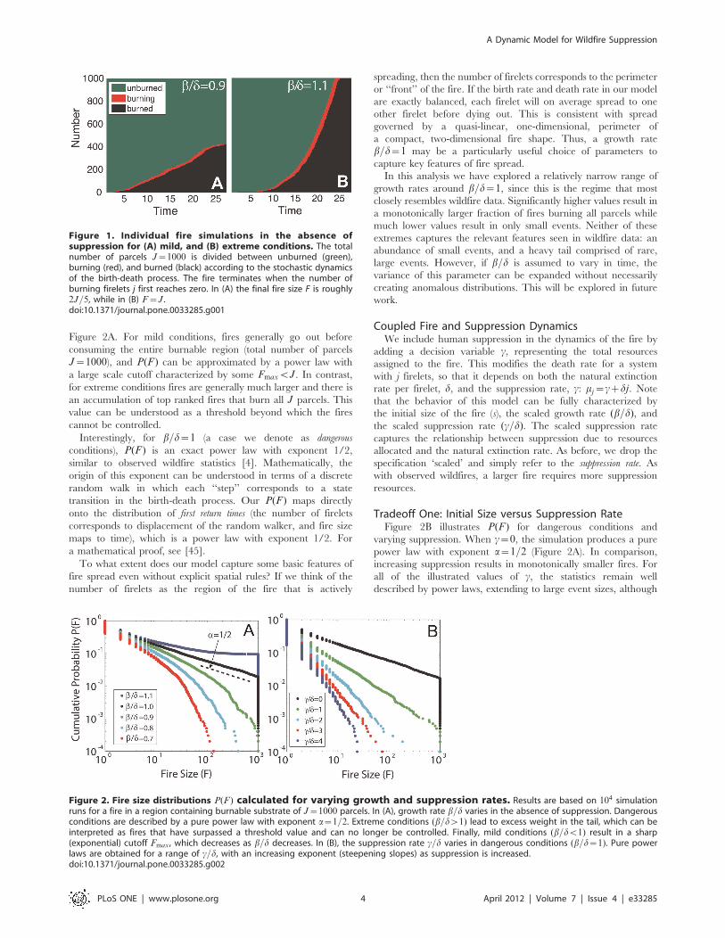
Figure 2A. For mild conditions, fires generally go out before

consuming the entire burnable region (total number of parcels

J~1000), and P(F ) can be approximated by a power law with

a large scale cutoff characterized by some FmaxvJ . In contrast,

for extreme conditions fires are generally much larger and there is

an accumulation of top ranked fires that burn all J parcels. This

value can be understood as a threshold beyond which the fires

cannot be controlled.

Interestingly, for b=d~1 (a case we denote as dangerous

conditions), P(F ) is an exact power law with exponent 1/2,

similar to observed wildfire statistics [4]. Mathematically, the

origin of this exponent can be understood in terms of a discrete

random walk in which each ‘‘step’’ corresponds to a state

transition in the birth-death process. Our P(F ) maps directly

onto the distribution of first return times (the number of firelets

corresponds to displacement of the random walker, and fire size

maps to time), which is a power law with exponent 1/2. For

a mathematical proof, see [45].

To what extent does our model capture some basic features of

fire spread even without explicit spatial rules? If we think of the

number of firelets as the region of the fire that is actively

spreading, then the number of firelets corresponds to the perimeter

or ‘‘front’’ of the fire. If the birth rate and death rate in our model

are exactly balanced, each firelet will on average spread to one

other firelet before dying out. This is consistent with spread

governed by a quasi-linear, one-dimensional, perimeter of

a compact, two-dimensional fire shape. Thus, a growth rate

b=d~1 may be a particularly useful choice of parameters to

capture key features of fire spread.

In this analysis we have explored a relatively narrow range of

growth rates around b=d~1, since this is the regime that most

closely resembles wildfire data. Significantly higher values result in

a monotonically larger fraction of fires burning all parcels while

much lower values result in only small events. Neither of these

extremes captures the relevant features seen in wildfire data: an

abundance of small events, and a heavy tail comprised of rare,

large events. However, if b=d is assumed to vary in time, the

variance of this parameter can be expanded without necessarily

creating anomalous distributions. This will be explored in future

work.

Coupled Fire and Suppression DynamicsWe include human suppression in the dynamics of the fire by

adding a decision variable c, representing the total resources

assigned to the fire. This modifies the death rate for a system

with j firelets, so that it depends on both the natural extinction

rate per firelet, d, and the suppression rate, c: mj~czdj. Note

that the behavior of this model can be fully characterized by

the initial size of the fire (s), the scaled growth rate (b=d), and

the scaled suppression rate (c=d). The scaled suppression rate

captures the relationship between suppression due to resources

allocated and the natural extinction rate. As before, we drop the

specification ‘scaled’ and simply refer to the suppression rate. As

with observed wildfires, a larger fire requires more suppression

resources.

Tradeoff One: Initial Size versus Suppression RateFigure 2B illustrates P(F ) for dangerous conditions and

varying suppression. When c~0, the simulation produces a pure

power law with exponent a~1=2 (Figure 2A). In comparison,

increasing suppression results in monotonically smaller fires. For

all of the illustrated values of c, the statistics remain well

described by power laws, extending to large event sizes, although

Figure 1. Individual fire simulations in the absence ofsuppression for (A) mild, and (B) extreme conditions. The totalnumber of parcels J~1000 is divided between unburned (green),burning (red), and burned (black) according to the stochastic dynamicsof the birth-death process. The fire terminates when the number ofburning firelets j first reaches zero. In (A) the final fire size F is roughly2J=5, while in (B) F~J .doi:10.1371/journal.pone.0033285.g001

Figure 2. Fire size distributions P(F ) calculated for varying growth and suppression rates. Results are based on 104 simulationruns for a fire in a region containing burnable substrate of J~1000 parcels. In (A), growth rate b=d varies in the absence of suppression. Dangerousconditions are described by a pure power law with exponent a~1=2. Extreme conditions (b=dw1) lead to excess weight in the tail, which can beinterpreted as fires that have surpassed a threshold value and can no longer be controlled. Finally, mild conditions (b=dv1) result in a sharp(exponential) cutoff Fmax, which decreases as b=d decreases. In (B), the suppression rate c=d varies in dangerous conditions (b=d~1). Pure powerlaws are obtained for a range of c=d, with an increasing exponent (steepening slopes) as suppression is increased.doi:10.1371/journal.pone.0033285.g002



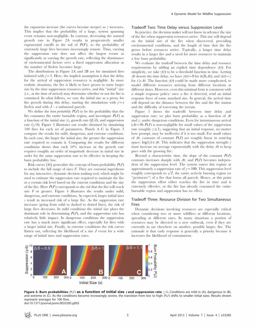
the exponents increase (the curves become steeper) as c increases.

This implies that the probability of a large, system spanning

event remains non-negligible. In contrast, decreasing the natural

growth rate in Figure 2A results in progressively smaller

exponential cutoffs in the tail of P(F), so the probability of

extremely large fires becomes increasingly remote. Thus, varying

the suppression rate does not affect the largest events as

significantly as varying the growth rate, reflecting the dominance

of environmental factors over a fixed suppression allocation as

the number of firelets becomes large.

The distributions in Figure 2A and 2B are for simulated fires

initiated with j~1. Here, the implicit assumption is that the delay

for the arrival of suppression resources is negligible. In more

realistic situations, the fire is likely to have grown to some larger

size by the time suppression resources arrive, and this ‘‘initial’’ size

(i.e., at the time of arrival) may determine whether or not the fire is

contained. In what follows, we vary the initial size as a proxy for

fire growth during this delay, starting the simulations with j~s

firelets and with J{s unburned parcels.

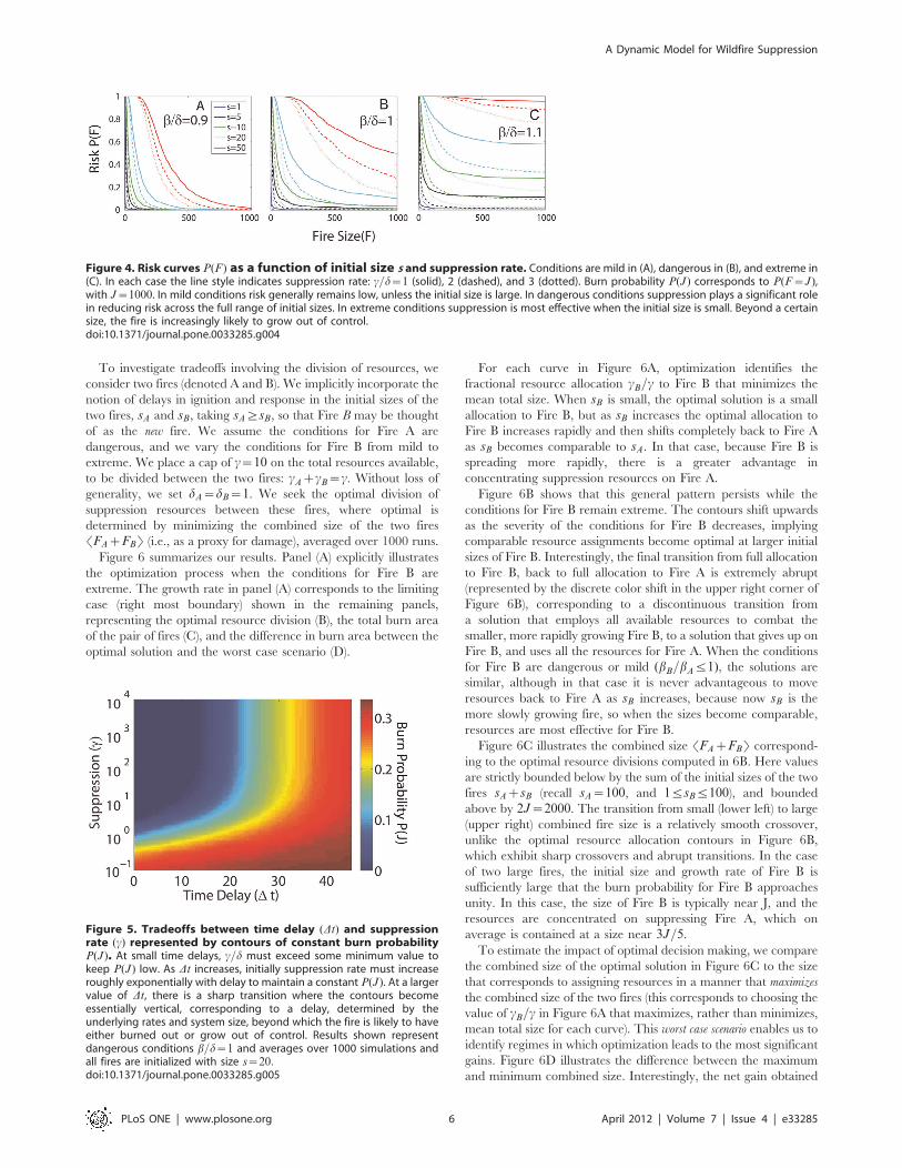
We define the burn probability P(J) to be the probability that the

fire consumes the entire burnable region, and investigate P(J) as

a function of the initial size (s), growth rate (b=d), and suppression

rate (c=d). Figure 3 illustrates our results obtained by simulating

100 fires for each set of parameters. Panels A–C in Figure 3

compare the results for mild, dangerous, and extreme conditions.

In each case, the larger the initial size, the greater the suppression

rate required to contain it. Comparing the results for different

conditions shows that each 10% increase in the growth rate

requires roughly an order of magnitude decrease in initial size in

order for the same suppression rate to be effective in keeping the

burn probability low.

Risk curves [46] generalize the concept of burn probability P(J)to include the full range of sizes F. They are essential ingredients

for any interactive, dynamic decision making tool, which might be

used to estimate the suppression rate required to maintain the fire

at a certain risk level based on the current conditions and the size

of the fire. Here P(F) corresponds to the risk that the fire will reach

size F or greater. Figure 4 illustrates the results under mild,

dangerous, and extreme conditions. As expected, larger initial sizes

s result in increased risk of a large fire. As the suppression rate

increases (going from solid to dashed to dotted lines), the risk of

large fires decreases. In mild conditions the initial size plays the

dominant role in determining P(J), and the suppression rate has

relatively little impact. In dangerous conditions the suppression

rate has a much more significant effect, especially for fires with

a larger initial size. Finally, in extreme conditions the risk curves

flatten out, reflecting the likelihood of a size J event for a wide

range of initial sizes and suppression rates.

Tradeoff Two: Time Delay versus Suppression LevelIn practice, the decision maker will not know in advance the size

of the fire when suppression resources arrive. This size will depend

on the initial size of the fire when discovered, prevailing

environmental conditions, and the length of time that the fire

grows before resources arrive. Typically, a longer time delay

results in a larger fire and a need for more resources to maintain

a low burn probability.

We evaluate the tradeoff between the time delay and resource

requirements by adding an explicit time dependence c(t). For

simplicity, we take c(t) to be a threshold function in time. Letting

Dt denote the time delay, we have c(t)~0 for t[½0,Dt), and c(t)~cfor t§Dt. The function c(t) could be made more complicated, to

model different resources arriving from different locations at

different times. However, even this minimal form is consistent with

a simple response policy: once a fire is detected, send an initial

response force of some standard size. In general, the arrival time

will depend on the distance between the fire and the fire station

and the difficulty of traversing the terrain.

Figure 5 shows the tradeoffs between time delay and

suppression rate; we plot burn probability as a function of Dtand c, under dangerous conditions. Even for instantaneous arrival

(Dt~0) P(J) is non-negligible for small values of the suppression

rate (roughly cƒ1), suggesting that an initial response, no matter

how prompt, may be ineffective if it is too small. For small values

of Dt, contours of constant P(J) are roughly linear in semi-log

space: log (c)!Dt. This indicates that the suppression strength cmust increase on average exponentially with the delay Dt to keep

pace with the growing fire.

Beyond a characteristic time, the slope of the constant P(J)contours increases sharply with Dt, and P(J) becomes indepen-

dent of the suppression level. The system enters this regime at

approximately a suppression rate of c~100. This suppression level

roughly corresponds toffiffiffi

Jp

, the entire actively burning region (or

‘‘perimeter’’) of a fire that burns all parcels. Hence, at this point

the suppression effort either reaches the fire in time and is

extremely effective, or the fire has already consumed the entire

burnable region and suppression has no effect.

Tradeoff Three: Resource Division for Two SimultaneousFires

Dynamic decisions involving resources are especially critical

when considering two or more wildfires at different locations,

spreading at different rates. In many situations a portion of

resources may be directed to a new outbreak, even if they are

currently in use elsewhere on another, possibly larger, fire. The

rationale is that early response is generally a priority because it

increases the likelihood of containment.

Figure 3. Burn probabilities P(J) as a function of initial size s and suppression rate c=d. Conditions are mild in (A), dangerous in (B),and extreme in (C). As the conditions become increasingly severe, the transition from low to high P(J) shifts to smaller initial sizes. Results shownrepresent averages for 100 fires.doi:10.1371/journal.pone.0033285.g003



To investigate tradeoffs involving the division of resources, we

consider two fires (denoted A and B). We implicitly incorporate the

notion of delays in ignition and response in the initial sizes of the

two fires, sA and sB, taking sA§sB, so that Fire B may be thought

of as the new fire. We assume the conditions for Fire A are

dangerous, and we vary the conditions for Fire B from mild to

extreme. We place a cap of c~10 on the total resources available,

to be divided between the two fires: cAzcB~c. Without loss of

generality, we set dA~dB~1. We seek the optimal division of

suppression resources between these fires, where optimal is

determined by minimizing the combined size of the two fires

SFAzFBT (i.e., as a proxy for damage), averaged over 1000 runs.

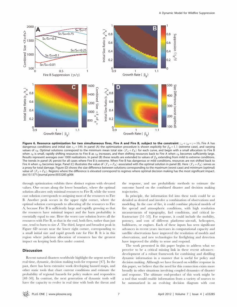
Figure 6 summarizes our results. Panel (A) explicitly illustrates

the optimization process when the conditions for Fire B are

extreme. The growth rate in panel (A) corresponds to the limiting

case (right most boundary) shown in the remaining panels,

representing the optimal resource division (B), the total burn area

of the pair of fires (C), and the difference in burn area between the

optimal solution and the worst case scenario (D).

For each curve in Figure 6A, optimization identifies the

fractional resource allocation cB=c to Fire B that minimizes the

mean total size. When sB is small, the optimal solution is a small

allocation to Fire B, but as sB increases the optimal allocation to

Fire B increases rapidly and then shifts completely back to Fire A

as sB becomes comparable to sA. In that case, because Fire B is

spreading more rapidly, there is a greater advantage in

concentrating suppression resources on Fire A.

Figure 6B shows that this general pattern persists while the

conditions for Fire B remain extreme. The contours shift upwards

as the severity of the conditions for Fire B decreases, implying

comparable resource assignments become optimal at larger initial

sizes of Fire B. Interestingly, the final transition from full allocation

to Fire B, back to full allocation to Fire A is extremely abrupt

(represented by the discrete color shift in the upper right corner of

Figure 6B), corresponding to a discontinuous transition from

a solution that employs all available resources to combat the

smaller, more rapidly growing Fire B, to a solution that gives up on

Fire B, and uses all the resources for Fire A. When the conditions

for Fire B are dangerous or mild (bB=bAƒ1), the solutions are

similar, although in that case it is never advantageous to move

resources back to Fire A as sB increases, because now sB is the

more slowly growing fire, so when the sizes become comparable,

resources are most effective for Fire B.

Figure 6C illustrates the combined size SFAzFBT correspond-

ing to the optimal resource divisions computed in 6B. Here values

are strictly bounded below by the sum of the initial sizes of the two

fires sAzsB (recall sA~100, and 1ƒsBƒ100), and bounded

above by 2J~2000. The transition from small (lower left) to large

(upper right) combined fire size is a relatively smooth crossover,

unlike the optimal resource allocation contours in Figure 6B,

which exhibit sharp crossovers and abrupt transitions. In the case

of two large fires, the initial size and growth rate of Fire B is

sufficiently large that the burn probability for Fire B approaches

unity. In this case, the size of Fire B is typically near J, and the

resources are concentrated on suppressing Fire A, which on

average is contained at a size near 3J=5.

To estimate the impact of optimal decision making, we compare

the combined size of the optimal solution in Figure 6C to the size

that corresponds to assigning resources in a manner that maximizes

the combined size of the two fires (this corresponds to choosing the

value of cB=c in Figure 6A that maximizes, rather than minimizes,

mean total size for each curve). This worst case scenario enables us to

identify regimes in which optimization leads to the most significant

gains. Figure 6D illustrates the difference between the maximum

and minimum combined size. Interestingly, the net gain obtained

Figure 4. Risk curves P(F ) as a function of initial size s and suppression rate. Conditions are mild in (A), dangerous in (B), and extreme in(C). In each case the line style indicates suppression rate: c=d~1 (solid), 2 (dashed), and 3 (dotted). Burn probability P(J) corresponds to P(F~J),with J~1000. In mild conditions risk generally remains low, unless the initial size is large. In dangerous conditions suppression plays a significant rolein reducing risk across the full range of initial sizes. In extreme conditions suppression is most effective when the initial size is small. Beyond a certainsize, the fire is increasingly likely to grow out of control.doi:10.1371/journal.pone.0033285.g004

Figure 5. Tradeoffs between time delay (Dt) and suppressionrate (c) represented by contours of constant burn probabilityP(J). At small time delays, c=d must exceed some minimum value tokeep P(J) low. As Dt increases, initially suppression rate must increaseroughly exponentially with delay to maintain a constant P(J). At a largervalue of Dt, there is a sharp transition where the contours becomeessentially vertical, corresponding to a delay, determined by theunderlying rates and system size, beyond which the fire is likely to haveeither burned out or grow out of control. Results shown representdangerous conditions b=d~1 and averages over 1000 simulations andall fires are initialized with size s~20:doi:10.1371/journal.pone.0033285.g005



through optimization exhibits three distinct regions with elevated

values. One occurs along the lower boundary, where the optimal

solution allocates only minimal resources to Fire B, while the worst

case solution corresponds to assigning most of the resources to Fire

B. Another peak occurs in the upper right corner, where the

optimal solution corresponds to allocating all the resources to Fire

A, because Fire B is sufficiently large and rapidly growing so that

the resources have minimal impact and the burn probability is

essentially equal to one. Here the worst case solution leaves all the

resources with Fire B, so that in the end, both fires, rather than just

one, tend to burn to size J: The third, largest and broadest peak in

Figure 6D occurs near the lower right corner, corresponding to

a small initial size and rapid growth rate for Fire B. It is in this

region where judicious allocation of resources has the greatest

impact on keeping both fires under control.

Discussion

Recent natural disasters worldwide highlight the urgent need for

real-time, dynamic, decision making tools for response [47]. In the

past, there has been extensive work developing hazard maps, and

other static tools that chart current conditions and estimate the

probability of regional hazards for policy makers and responders

[48–50]. In contrast, the next generation of dynamic tools will

have the capacity to evolve in real time with both the threat and

the response, and use probabilistic methods to estimate the

outcome based on the combined disaster and decision making

trajectories.

In principle, the information fed into these tools could be as

detailed as desired and involve a combination of observations and

modeling. In the case of fire, it could combine physical models of

fire spread and atmospheric conditions, with high resolution

measurements of topography, fuel conditions, and critical in-

frastructure [51–53]. For response, it could include the mobility,

potency, and cost of different platforms–aircraft, helicopters,

bulldozers, or engines. Each of these inputs has seen significant

advances in recent years–increases in computational capacity and

satellite observations have improved the resolution of models and

observations, and new technologies for firefighting and detection

have improved the ability to sense and respond.

The work presented in this paper begins to address what we

perceive to be a critical missing link in these recent advances–

development of a robust framework for combining and distilling

dynamic information in a manner that is useful for policy and

decision making. Although we have focused on wildfire response in

this paper, we believe that the need for this connection exists more

broadly in other situations involving coupled dynamics of disaster

and response. The ultimate end-product of this work might be

a tool that would enable information from a variety of sources to

be summarized in an evolving decision diagram with cost

Figure 6. Resource optimization for two simultaneous fires, Fire A and Fire B, subject to the constraint cAzcB~c~10. Fire A hasdangerous conditions and initial size sA~100. In panel (A) the optimization procedure is shown explicitly for bB~1:1 (extreme case), and varyingvalues of sB. Optimal solutions correspond to the minimum mean total size SFAzFBT for each curve, and begin with a small allocation to Fire Bwhen sB is small, rapidly shifting resources to Fire B as sB increases, and then shifting resources back to Fire A when sB becomes sufficiently large.Results represent averages over 1000 realizations. In panel (B) these results are extended to values of bB extending from mild to extreme conditions.The trends in panel (A) persist for all cases where Fire B is extreme. When Fire B has dangerous or mild conditions, resources are not shifted back toFire A when sB becomes large. Panel (C) illustrates the value of SFAzFBT associated with the optimal solution in panel (B). Here SFAzFBT serves asa proxy for total damage. Figure (D) shows the size difference between solutions corresponding to the maximum (worst case) and minimum (optimal)value of SFAzFBT. Regions where the difference is elevated correspond to regimes where optimal decision making has the most significant impact.doi:10.1371/journal.pone.0033285.g006



projections carried forward over a user-designated time interval.

For example, such a diagram might summarize model and

observation based projections, constrained by resource availability

and effectiveness, while the user considers deployment in different

locations at specific times. In the context of the work presented

here, our input parameters: the natural growth b and extinction drates, the initial size s, and the suppression allocation c represent

real-time inputs based on current conditions, models, and policy

decisions, with dynamic outputs, analogous to our probability

contours, highlighting the essential tradeoffs and estimating risks

over various time scales.

Of course, a great deal must be done before such complex

analysis can be automated. Current capabilities to observe and

model greatly exceed the capacity to distill and integrate results in

a manner that is comprehensible, efficient, and robust for policy.

Any effort to compress information is inherently delicate because

of the intrinsic fragilities associated with cascading breakdowns

initiated by one small failure. This motivates our approach, based

on deliberately transparent models and isolated tradeoffs, aimed at

clarifying fundamental issues that arise generally in this class of

problems.

In these first steps of developing a decision making framework

for policy, it is less crucial to capture every detail of wildfire

dynamics than it is to correctly represent those features that are

resolved in the initial, coarse representation that is used–in this

case spread rates consistent with compact fire footprints and the

resulting statistical distribution of sizes. Such features are expected

to persist as more detailed models are incorporated into the

framework. In contrast, a framework based on a model that does

not get the simple things right is likely to produce misleading

results from the start. More detailed models of fire spread retain

compact shapes and statistical features, while incorporating

additional features (e.g., topography and fuel type), and exposing

additional sensitivities (e.g., winds and humidity) that are

important for fire spread.

This work suggests many directions for future research–

integration with geospatial approaches, increases in fire and

response model resolution, and more accurate, data-driven

incorporation of physical parameters. In the case of California

wildfires, a dominant factor is wind. The largest, most destructive

wildfires are typically associated with extreme, high wind, low

humidity Santa Ana conditions [54,55]. Fluctuations in wind

speeds during these events dominate both the dynamics of fire

spread and the effectiveness of response. Even in our abstract

model, this could be represented by time dependent birth and

death rates for fire spread, to evaluate the optimal time

dependence for effective response.

Current decision making for wildfire relies on a combination of

protocols established in advance and real-time expert opinion. A

great deal of data is available to facilitate these decisions. In some

cases, it may be even too much, resulting in information overload.

The purpose of investigations such as ours is not to replace the

experts, but rather to provide them with a sound, statistical basis

for synthesizing information, establishing protocols, and predicting

system sensitivities in advance.

Acknowledgments

The authors thank Danielle Bassett, Emily Craparo, and John Doyle for

helpful discussions.

Author Contributions

Conceived and designed the experiments: NP DLA JMC. Performed the

experiments: NP DLA JMC. Analyzed the data: NP DLA JMC.

Contributed reagents/materials/analysis tools: NP DLA JMC. Wrote the

paper: NP DLA JMC.

References

1. Perry GLW (1998) Current approaches to modelling the spread of wildland fire:

A review. Progress in Physical Geography 22: 222–245.

2. Weber RO (1991) Modelling fire spread through fuel beds. Progress in Energy

and Combustion Science 17: 67–82.

3. Barbour MG, Burk JH, Pitts WD (1987) Terrestrial plant ecology, 2nd edition.

Menlo Park: Benjamin Cummins.

4. Moritz MA, Morais ME, Summerell LA, Carlson JM, Doyle J (2005) Wildfires,

complexity, and highly optimized tolerance. Proceedings of the National

Academy of Sciences of the United States of America 102: 17912–17917.

5. California Department of Forestry and Fire Protection: Statistics and events.

Available: http://cdfdata.fire.ca.gov/incidents/incidents statsevents. Accessed

2012 March, 10.

6. Big burn: The Times explores the growth and cost of wildfires. Available:

http://www.latimes.com/news/local/la-me-fire-index,0,4857752.htmlstory.

Accessed 2012 March, 10.

7. Gebert KM, Calkin DE, Yoder J (2007) Estimating suppression expenditures for

individual large wildland fires. Western Journal of Applied Forestry 22: 188–196.

8. Calkin DE, Gebert KM, Jones JG, Neilson RP (2005) Forest service large fire

area burned and suppression expenditure trends, 1970–2002. Journal of Forestry

103: 179–183.

9. Westerling AL, Hidalgo HG, Cayan DR, Swetnam TW (2006) Warming and

earlier spring increase western U.S. forest wildfire activity. Science 313:

940–943.

10. Westerling AL, Gershunov A, Brown TJ, Cayan DR, Dettinger MD (2003)

Climate and wildfire in the western United States. Bulletin of the American

Meteorological Society 84: 595–604.

11. Swetnam TW, Betancourt JL (1998) Mesoscale disturbance and ecological

response to decadal climatic variability in the American Southwest. Journal of

Climate 11: 3128–3147.

12. Snyder GW (1999) Strategic holistic integrated planning for the future: Fire

protection in the urban/rural/wildland interface (URWIN). General Technical

Report PSW-GTR-173, U.S. Department of Agriculture, Forest Service, Pacific

Southwest Research Station, San Diego, CA.

13. Radeloff VC, Hammer RB, Stewart SI, Fried JS, Holcomb SS, et al. (2005) The

wildland-urban interface in the United States. Ecological Applications 15:

799–805.

14. Islam KMS, Martell DL (1998) Performance of initial attack airtanker systems

with interacting bases and variable initial attack ranges. Canadian Journal of

Forest Research 28: 1448–1455.

15. Bookbinder JH, Martell DL (1979) Time-dependent queueing approach to

helicopter allocation for forest fire initial-attack. INFOR: Information Systems

and Operational Research 17: 58–70.

16. Martin-Fernandez S, Martınez-Falero E, Perez-Gonzalez JM (2002) Optimiza-

tion of the resources management in fighting wildfires. Environmental

Management 30: 352–364.

17. Donovan GH, Rideout DB (2003) An integer programming model to optimize

resource allocation for wildfire containment. Forest Science 49: 331–335.

18. Martell DL (1982) A review of operational research studies in forest fire

management. Canadian Journal of Forest Research 12: 119–140.

19. Haight RG, Fried JS (2007) Deploying wildland fire suppression resources with

a scenario-based standard response model. INFOR: Information Systems and

Operational Research 45: 31–39.

20. Pisarenko V, Rodkin M (2010) Heavy-tailed distributions in disaster analysis.

New York: Springer, 1–21 pp.

21. Hergarten S (2004) Aspects of risk assessment in power-law distributed natural

hazards. Natural Hazards and Earth System Science 4: 309–313.

22. Mitzenmacher M (2004) A brief history of generative models for power law and

lognormal distributions. Internet Mathematics 1: 226–251.

23. Sornette D (2006) Critical phenomena in natural sciences, 2nd edition. Berlin:

Springer.

24. Newman MEJ (2010) Networks: An introduction. New York: Oxford University

Press.

25. Bak P (1996) How nature works: The science of self-organized criticality. New

York: Copernicus.

26. Barabasi AL (2002) Linked: The new science of networks. Cambridge: Perseus

Publishing.

27. Willinger W, Alderson DA, Doyle JC, Li L (2004) More ‘‘normal’’ than normal:

Scaling distributions and complex systems. In: Ingalls RG, Rossetti MD, Smith

JS, Peters BA, editors, Proceedings of the 2004 Winter Simulation Conference,

New York: ACM Press. pp 130–141.

28. Strauss D, Bednar L, Mees R (1989) Do one percent of forest fires cause ninety-

nine percent of the damage? Forest Science 35: 319–328.



29. Malamud BD, Morein G, Turcotte DL (1998) Forest fires: An example of self-

organized critical behavior. Science 281: 1840–1842.30. Corral A, Osso A, Llebot J (2010) Scaling of tropical-cyclone dissipation. Nature

Physics 6: 693–696.

31. Gutenberg B, Richter CF (1954) Seismicity of the earth and associatedphenomena, 2nd edition. Princeton: Princeton University Press.

32. Chen K, Bak P, Jensen MH (1990) A deterministic critical forest fire model.Physics Letters A 149: 207–210.

33. Drossel B, Schwabl F (1992) Self-organized critical forest-fire model. Physical

Review Letters 69: 1629–1632.34. Stauffer D, Aharony A (1992) Introduction to percolation theory, 2nd edition.

London: Taylor and Francis.35. Carlson JM, Doyle J (2000) Power laws, highly optimized tolerance, and

generalized source coding. Physical Review Letters 84: 5656–5659.36. Christensen GA, Campbell SJ, Fried JS (2008) California’s forest resources,

2001–2005: Five-year forest inventory and analysis report. General Technical

Report PNW-GTR-763, U.S. Department of Agriculture, Forest Service, PacificNorthwest Research Station, Portland, OR.

37. California Department of Forestry and Fire Protection: Surface fuels maps anddata. Available: http://frap.cdf.ca.gov/data/fire data/fuels/fuelsfr.html. Ac-

cessed 2012 March, 10.

38. Anderson HE (1983) Predicting wind-driven wild land fire size and shape.Research Paper INT-305, U.S. Department of Agriculture, Forest Service,

Intermountain Forest and Range Experiment Station, Ogden, UT.39. Carlson JM, Doyle J (1999) Highly optimized tolerance: A mechanism for power

laws in designed systems. Physical Review E 60: 1412–1427.40. Carlson JM, Doyle J (2002) Complexity and robustness. Proceedings of the

National Academy of Sciences of the United States of America 99: 2538–2545.

41. Peterson SH, Morais ME, Carlson JM, Dennison PE, Roberts DA, et al. (2009)Using HFire for spatial modeling of fire in shrublands. Research Paper PSW-

RP-259, U.S. Department of Agriculture, Forest Service, Pacific SouthwestResearch Station, Albany, CA.

42. Peterson SH, Moritz MA, Morais ME, Dennison PE, Carlson JM (2011)

Modelling long-term fire regimes of southern California shrublands. Interna-tional Journal of Wildland Fire 20: 1–16.

43. Rothermel RC (1972) A mathematical model for predicting fire spread inwildland fuels. Research Paper INT-115, U.S. Department of Agriculture,

Forest Service, Intermountain Forest and Range Experiment Station, Ogden,

UT.

44. Rothermel RC (1983) How to predict the spread and intensity of forest and

range fires. General Technical Report INT-143, U.S. Department of

Agriculture, Forest Service, Intermountain Forest and Range Experiment

Station, Ogden, UT.

45. Newman MEJ (2005) Power laws, Pareto distributions and Zipf’s law.

Contemporary Physics 46: 323–351.

46. Kaplan S, Garrick BJ (1981) On the quantitative definition of risk. Risk Analysis

1: 11–27.

47. Centre for Research on the Epidemiology of Disasters: 2010 disasters in

numbers. Available: http://cred.be/sites/default/files/PressConference2010.

pdf. Accessed 2012 March, 10.

48. United States Geological Survey hazard mapping images and data. Available at:

http://earthquake.usgs.gov/hazards/products/. Accessed 2012 March, 10.

49. California Department of Forestry and Fire Protection: Fire hazard maps.

Available: http://frap.cdf.ca.gov/data/frapgismaps/select.asp?theme = 5. Ac-

cessed 2012 March, 10.

50. National Oceanic and Atmospheric Administration: National weather hazards

map. Available: http://www.weather.gov/largemap.php. Accessed 2012

March, 10.

51. Finney MA, Grenfell IC, McHugh CW, Seli RC, Trethewey D, et al. (2011) A

method for ensemble wildland fire simulation. Environmental Modeling and

Assessment 16: 153–167.

52. Calkin DE, Rieck JD, Hyde KD, Kaiden JD (2011) Built structure identification

in wildland fire decision support. International Journal of Wildland Fire 20:

78–90.

53. Calkin DE, Thompson MP, Finney MA, Hyde KD (2011) A real-time risk

assessment tool supporting wildland fire decisionmaking. Journal of Forestry

109: 274–280.

54. Moritz MA (1997) Analyzing extreme disturbance events: Fire in Los Padres

National Forest. Ecological Applications 7: 1252–1262.

55. Davis FW, Michaelsen J (1995) Sensitivity of fire regime in chaparral ecosystems

to climate change. In: Moreno JM, OechelWC, editors, Global change and

Mediterranean-type ecosystems, New York: Springer. pp 203–224.



Documents

Dynamic Resource Allocation in Disaster Response ...web.physics.ucsb.edu/~complex/pubs/Dynamic Resource Allocation … · Dynamic Resource Allocation in Disaster Response: Tradeoffs