
University of Massachusetts Amherst University of Massachusetts Amherst
ScholarWorks@UMass Amherst ScholarWorks@UMass Amherst
Open Access Dissertations
9-2011
Computational Affect Detection for Education and Health Computational Affect Detection for Education and Health
David G. Cooper University of Massachusetts Amherst, [email protected]
Follow this and additional works at: https://scholarworks.umass.edu/open_access_dissertations
Part of the Computer Sciences Commons
Recommended Citation Recommended Citation Cooper, David G., "Computational Affect Detection for Education and Health" (2011). Open Access Dissertations. 437. https://scholarworks.umass.edu/open_access_dissertations/437
This Open Access Dissertation is brought to you for free and open access by ScholarWorks@UMass Amherst. It has been accepted for inclusion in Open Access Dissertations by an authorized administrator of ScholarWorks@UMass Amherst. For more information, please contact [email protected].

COMPUTATIONAL AFFECT DETECTION FOREDUCATION AND HEALTH
A Dissertation Presented
by
DAVID G. COOPER
Submitted to the Graduate School of theUniversity of Massachusetts Amherst in partial fulfillment
of the requirements for the degree of
DOCTOR OF PHILOSOPHY
September 2011
Computer Science

c© Copyright by David G. Cooper 2011
All Rights Reserved

COMPUTATIONAL AFFECT DETECTION FOREDUCATION AND HEALTH
A Dissertation Presented
by
DAVID G. COOPER
Approved as to style and content by:
Hava T. Siegelmann, Co-chair
Beverly Park Woolf, Co-chair
Andrew G. Barto, Member
Mary Andrianopoulos, Member
Andrew G. Barto, Department ChairComputer Science

To my beloved wife, Erin, and son, Isaac, who inspire me daily.

ACKNOWLEDGEMENTS
I’d like to thank my committee for believing in my research and helping me hone
in on my topic. Specifically, I acknowledge my advisor Hava T. Siegelmann, who
encouraged me to return to academia to work with her, and who helped me translate
my initial thesis idea into a reality. My foundation in computational emotion began
with Hava’s course on the subject. I acknowledge my advisor Beverly Park Woolf who
introduced me to the intricacies of educational technology, and who helped me become
part of the artificial intelligence in education research community. Beverly’s feedback
and encouragement have made the process of writing a dissertation much smoother.
I also would like to thank my other committee members Andy Barto, who helped me
frame this work into the field of computer science, and Mary Andrianopoulos whose
insight into voice production and whose meticulous data collection methods made my
work in audio processing accessible.
I would also like to thank Helene Cunningham who is in charge of the clinical
simulation environment, and who helped me determine how to feasibly conduct a
study in the lab space. Mary Ann Hogan and Kimberly Dion were very generous in
allowing me access to their students for the study.
I acknowledge contributions to the system development of the educational sensors
from Rana el Kaliouby, Winslow Burleson, Kasia Muldner, Ashish Kapoor, Selene
Mota and Carson Reynolds. I also thank Joshua Richman, Roopesh Konda, and
Assegid Kidane at ASU for their work on sensor manufacturing. I thank Sharon
Edwards and Sarah English for their coordination of the school studies.
v

The administrative of the computer science department have helped me handle
the necessary paperwork to work and travel. Gwyn Mitchel and Leeanne Leclerc were
especially helpful to me.
The CSCF staff were very helpful in keeping the swarm and my work computer up
and running. This research benefited from the use of the UMass CS swarm cluster sup-
ported in part by the National Science Foundation under NSF grant #CNS-0619337.
The computer based education research was funded by awards from the National
Science Foundation, 0705554, IIS/HCC Affective Learning Companions: Modeling
and Supporting Emotion During Teaching, Woolf and Burleson (PIs) with Arroyo,
Barto, and Fisher and the U.S. Department of Education to Woolf, B. P. (PI) with
Arroyo, Maloy and the Center for Applied Special Technology (CAST), Teaching
Every Student: Using Intelligent Tutoring and Universal Design To Customize The
Mathematics Curriculum. Any opinions, findings, conclusions or recommendations
expressed in this material are those of the authors and do not necessarily reflect the
views of the funding agencies.
The entire Computer Science faculty at the University of Massachusetts improved
my foundation in computer science. In addition to my committee, conversations
with Oliver Brock, Rod Grupen, David Jensen, and Erik Learned-Miller, as well
as courses from Rod Grupen, David Jensen, Erik Learned-Miller, Neil Immerman,
Sridhar Mahadevan, Prashant Shenoy, Ramesh Sitaraman, and Paul Utgoff helped
frame my perspective on computer science.
I have benefited from many lunch conversations with fellow students as well as
conversations in the labs that I have had a desk. I would especially like to thank
Megan Olsen and Yariv Levy, who have been a constant support from when I started
in the BINDS lab.
I’d like to thank my wife Erin, for dropping her life in Philadelphia, and moving
here so that I could pursue my Ph.D.
vi
ABSTRACT
COMPUTATIONAL AFFECT DETECTION FOREDUCATION AND HEALTH
SEPTEMBER 2011
DAVID G. COOPER
B.S., CARNEGIE MELLON UNIVERSITY
M.S., UNIVERSITY OF MASSACHUSETTS AMHERST
Ph.D., UNIVERSITY OF MASSACHUSETTS AMHERST
Directed by: Professor Hava T. Siegelmann and Professor Beverly Park Woolf
Emotional intelligence has a prominent role in education, health care, and day
to day interaction. With the increasing use of computer technology, computers are
interacting with more and more individuals. This interaction provides an opportunity
to increase knowledge about human emotion for human consumption, well-being, and
improved computer adaptation. This thesis explores the efficacy of using up to four
different sensors in three domains for computational affect detection. We first consider
computer-based education, where a collection of four sensors is used to detect student
emotions relevant to learning, such as frustration, confidence, excitement and interest
while students use a computer geometry tutor. The best classier of each emotion in
terms of accuracy ranges from 78% to 87.5%. We then use voice data collected in a
clinical setting to differentiate both gender and culture of the speaker. We produce
classifiers with accuracies between 84% and 94% for gender, and between 58% and
vii

70% for American vs. Asian culture, and we find that classifiers for distinguishing
between four cultures do not perform better than chance. Finally, we use video
and audio in a health care education scenario to detect students’ emotions during
a clinical simulation evaluation. The video data provides classifiers with accuracies
between 63% and 88% for the emotions of confident, anxious, frustrated, excited,
and interested. We find the audio data to be too complex to single out the voice
source of the student by automatic means. In total, this work is a step forward in
the automatic computational detection of affect in realistic settings.
viii

TABLE OF CONTENTS
Page
ACKNOWLEDGEMENTS . . . . . . . . . . . . . . . . . . . . . . . . . . . . . . . . . . . . . . . . . . . v
ABSTRACT . . . . . . . . . . . . . . . . . . . . . . . . . . . . . . . . . . . . . . . . . . . . . . . . . . . . . . . . . vii
LIST OF TABLES . . . . . . . . . . . . . . . . . . . . . . . . . . . . . . . . . . . . . . . . . . . . . . . . . . .xiii
LIST OF FIGURES . . . . . . . . . . . . . . . . . . . . . . . . . . . . . . . . . . . . . . . . . . . . . . . . . . xvi
CHAPTER
1. INTRODUCTION . . . . . . . . . . . . . . . . . . . . . . . . . . . . . . . . . . . . . . . . . . . . . . . . . 1
1.1 Why Study Affect . . . . . . . . . . . . . . . . . . . . . . . . . . . . . . . . . . . . . . . . . . . . . . . . 21.2 The Study of Affect . . . . . . . . . . . . . . . . . . . . . . . . . . . . . . . . . . . . . . . . . . . . . . . 4
1.2.1 Affective Channels and Labels . . . . . . . . . . . . . . . . . . . . . . . . . . . . . . . 4
1.2.1.1 Faces . . . . . . . . . . . . . . . . . . . . . . . . . . . . . . . . . . . . . . . . . . . . . 51.2.1.2 Voices . . . . . . . . . . . . . . . . . . . . . . . . . . . . . . . . . . . . . . . . . . . . 61.2.1.3 Physiology . . . . . . . . . . . . . . . . . . . . . . . . . . . . . . . . . . . . . . . . 81.2.1.4 Movement . . . . . . . . . . . . . . . . . . . . . . . . . . . . . . . . . . . . . . . . . 8
1.2.2 Affect Classification . . . . . . . . . . . . . . . . . . . . . . . . . . . . . . . . . . . . . . . . 91.2.3 Target Applications . . . . . . . . . . . . . . . . . . . . . . . . . . . . . . . . . . . . . . . 12
1.3 Contributions . . . . . . . . . . . . . . . . . . . . . . . . . . . . . . . . . . . . . . . . . . . . . . . . . . . 121.4 Thesis Outline . . . . . . . . . . . . . . . . . . . . . . . . . . . . . . . . . . . . . . . . . . . . . . . . . . 13
2. BACKGROUND . . . . . . . . . . . . . . . . . . . . . . . . . . . . . . . . . . . . . . . . . . . . . . . . . 15
2.1 Affective Sensors . . . . . . . . . . . . . . . . . . . . . . . . . . . . . . . . . . . . . . . . . . . . . . . . 15
2.1.1 Education Use . . . . . . . . . . . . . . . . . . . . . . . . . . . . . . . . . . . . . . . . . . . . 15
2.1.1.1 Skin Conductance Bracelet . . . . . . . . . . . . . . . . . . . . . . . . . 15
ix

2.1.1.2 Pressure Sensitive Mouse . . . . . . . . . . . . . . . . . . . . . . . . . . . 152.1.1.3 Pressure Sensitive Chair . . . . . . . . . . . . . . . . . . . . . . . . . . . 162.1.1.4 Mental State Camera . . . . . . . . . . . . . . . . . . . . . . . . . . . . . . 16
2.1.2 Voice Sensors . . . . . . . . . . . . . . . . . . . . . . . . . . . . . . . . . . . . . . . . . . . . . 17
2.1.2.1 Voice in Health . . . . . . . . . . . . . . . . . . . . . . . . . . . . . . . . . . . 172.1.2.2 Voice in Emotion . . . . . . . . . . . . . . . . . . . . . . . . . . . . . . . . . . 172.1.2.3 Voice in Culture . . . . . . . . . . . . . . . . . . . . . . . . . . . . . . . . . . 18
2.1.3 Video Sensors . . . . . . . . . . . . . . . . . . . . . . . . . . . . . . . . . . . . . . . . . . . . . 19
2.2 Classification as Prediction . . . . . . . . . . . . . . . . . . . . . . . . . . . . . . . . . . . . . . . 20
2.2.1 Ideal Conditions . . . . . . . . . . . . . . . . . . . . . . . . . . . . . . . . . . . . . . . . . . 202.2.2 Deviations from the ideal . . . . . . . . . . . . . . . . . . . . . . . . . . . . . . . . . . . 21
2.3 Classification Methods . . . . . . . . . . . . . . . . . . . . . . . . . . . . . . . . . . . . . . . . . . . 21
3. USER MODEL FOR COMPUTER BASED EDUCATION . . . . . . . . 23
3.1 Related Work . . . . . . . . . . . . . . . . . . . . . . . . . . . . . . . . . . . . . . . . . . . . . . . . . . . 243.2 Affect Detection System . . . . . . . . . . . . . . . . . . . . . . . . . . . . . . . . . . . . . . . . . . 25
3.2.1 The Tutor: Wayang Outpost . . . . . . . . . . . . . . . . . . . . . . . . . . . . . . . . 253.2.2 Sensor Features . . . . . . . . . . . . . . . . . . . . . . . . . . . . . . . . . . . . . . . . . . . 27
3.2.2.1 Mouse Feature . . . . . . . . . . . . . . . . . . . . . . . . . . . . . . . . . . . . 283.2.2.2 Chair Features . . . . . . . . . . . . . . . . . . . . . . . . . . . . . . . . . . . . 293.2.2.3 Bracelet Feature . . . . . . . . . . . . . . . . . . . . . . . . . . . . . . . . . . 303.2.2.4 Mental State Camera Features . . . . . . . . . . . . . . . . . . . . . . 30
3.2.3 Feature Integration . . . . . . . . . . . . . . . . . . . . . . . . . . . . . . . . . . . . . . . . 30
3.3 Experimental Setup . . . . . . . . . . . . . . . . . . . . . . . . . . . . . . . . . . . . . . . . . . . . . . 323.4 Affect Classifiers . . . . . . . . . . . . . . . . . . . . . . . . . . . . . . . . . . . . . . . . . . . . . . . . . 33
3.4.1 Cross-Validation of the Linear Models . . . . . . . . . . . . . . . . . . . . . . . . 35
3.5 Discussion . . . . . . . . . . . . . . . . . . . . . . . . . . . . . . . . . . . . . . . . . . . . . . . . . . . . . . 36
4. RANKING CLASSIFIERS FOR COMPUTER BASEDEDUCATION . . . . . . . . . . . . . . . . . . . . . . . . . . . . . . . . . . . . . . . . . . . . . . . . . 37
4.1 Introduction . . . . . . . . . . . . . . . . . . . . . . . . . . . . . . . . . . . . . . . . . . . . . . . . . . . . 374.2 Related Work . . . . . . . . . . . . . . . . . . . . . . . . . . . . . . . . . . . . . . . . . . . . . . . . . . . 384.3 Data Collection: Sensors with Wayang Outpost in the Classroom . . . . . . 40
x

4.3.1 Setup . . . . . . . . . . . . . . . . . . . . . . . . . . . . . . . . . . . . . . . . . . . . . . . . . . . . 404.3.2 Tutor and Sensor Features . . . . . . . . . . . . . . . . . . . . . . . . . . . . . . . . . . 42
4.4 Method . . . . . . . . . . . . . . . . . . . . . . . . . . . . . . . . . . . . . . . . . . . . . . . . . . . . . . . . 42
4.4.1 Collection . . . . . . . . . . . . . . . . . . . . . . . . . . . . . . . . . . . . . . . . . . . . . . . . 444.4.2 Predictor Selection . . . . . . . . . . . . . . . . . . . . . . . . . . . . . . . . . . . . . . . . 444.4.3 Cross-Validation . . . . . . . . . . . . . . . . . . . . . . . . . . . . . . . . . . . . . . . . . . 444.4.4 Classifier Ranking . . . . . . . . . . . . . . . . . . . . . . . . . . . . . . . . . . . . . . . . . 454.4.5 Validation with Follow-on Data . . . . . . . . . . . . . . . . . . . . . . . . . . . . . 46
4.5 Results . . . . . . . . . . . . . . . . . . . . . . . . . . . . . . . . . . . . . . . . . . . . . . . . . . . . . . . . . 46
4.5.1 Classifier Ranking . . . . . . . . . . . . . . . . . . . . . . . . . . . . . . . . . . . . . . . . . 484.5.2 Validation with Follow-on Data . . . . . . . . . . . . . . . . . . . . . . . . . . . . . 50
4.6 Discussion . . . . . . . . . . . . . . . . . . . . . . . . . . . . . . . . . . . . . . . . . . . . . . . . . . . . . . 50
5. SPEAKER DIFFERENCES AND HEALTH DIAGNOSIS . . . . . . . . 53
5.1 Related Work . . . . . . . . . . . . . . . . . . . . . . . . . . . . . . . . . . . . . . . . . . . . . . . . . . . 535.2 Experimental Setup : Multicultural Study . . . . . . . . . . . . . . . . . . . . . . . . . . 555.3 Classification. . . . . . . . . . . . . . . . . . . . . . . . . . . . . . . . . . . . . . . . . . . . . . . . . . . . 565.4 Results . . . . . . . . . . . . . . . . . . . . . . . . . . . . . . . . . . . . . . . . . . . . . . . . . . . . . . . . . 575.5 Discussion and Future Work . . . . . . . . . . . . . . . . . . . . . . . . . . . . . . . . . . . . . . 59
6. HEALTH CARE EDUCATION . . . . . . . . . . . . . . . . . . . . . . . . . . . . . . . . . . . 61
6.1 Clinical Simulation . . . . . . . . . . . . . . . . . . . . . . . . . . . . . . . . . . . . . . . . . . . . . . 616.2 Experimental Setup . . . . . . . . . . . . . . . . . . . . . . . . . . . . . . . . . . . . . . . . . . . . . . 626.3 Video Features . . . . . . . . . . . . . . . . . . . . . . . . . . . . . . . . . . . . . . . . . . . . . . . . . . 63
6.3.1 Feature Extraction . . . . . . . . . . . . . . . . . . . . . . . . . . . . . . . . . . . . . . . . 646.3.2 Affect Classification . . . . . . . . . . . . . . . . . . . . . . . . . . . . . . . . . . . . . . . 656.3.3 Pre-processing . . . . . . . . . . . . . . . . . . . . . . . . . . . . . . . . . . . . . . . . . . . . 66
6.3.3.1 Person Tracking . . . . . . . . . . . . . . . . . . . . . . . . . . . . . . . . . . 666.3.3.2 Tracking Algorithm . . . . . . . . . . . . . . . . . . . . . . . . . . . . . . . 706.3.3.3 Tracking algorithm variants . . . . . . . . . . . . . . . . . . . . . . . . 73
6.3.4 Tracking Comparison . . . . . . . . . . . . . . . . . . . . . . . . . . . . . . . . . . . . . . 766.3.5 Tracking Results . . . . . . . . . . . . . . . . . . . . . . . . . . . . . . . . . . . . . . . . . . 766.3.6 Video Events . . . . . . . . . . . . . . . . . . . . . . . . . . . . . . . . . . . . . . . . . . . . . 76
6.3.6.1 Feature Selection . . . . . . . . . . . . . . . . . . . . . . . . . . . . . . . . . . 79
6.4 Voice Features . . . . . . . . . . . . . . . . . . . . . . . . . . . . . . . . . . . . . . . . . . . . . . . . . . 81
xi

6.4.1 Future work . . . . . . . . . . . . . . . . . . . . . . . . . . . . . . . . . . . . . . . . . . . . . 82
6.5 Discussion & Future Work . . . . . . . . . . . . . . . . . . . . . . . . . . . . . . . . . . . . . . . . 82
7. DISCUSSION AND FUTURE WORK . . . . . . . . . . . . . . . . . . . . . . . . . . . . 84
7.1 Hypotheses Revisited . . . . . . . . . . . . . . . . . . . . . . . . . . . . . . . . . . . . . . . . . . . . 847.2 Lessons Learned and Future Directions . . . . . . . . . . . . . . . . . . . . . . . . . . . . . 86
7.2.1 Computer Based Education . . . . . . . . . . . . . . . . . . . . . . . . . . . . . . . . . 86
7.2.1.1 Sensors . . . . . . . . . . . . . . . . . . . . . . . . . . . . . . . . . . . . . . . . . 867.2.1.2 Controls . . . . . . . . . . . . . . . . . . . . . . . . . . . . . . . . . . . . . . . . . 877.2.1.3 Feedback . . . . . . . . . . . . . . . . . . . . . . . . . . . . . . . . . . . . . . . . 87
7.2.2 Speaker Differences and Health Diagnosis . . . . . . . . . . . . . . . . . . . . . 87
7.2.2.1 Classifiers . . . . . . . . . . . . . . . . . . . . . . . . . . . . . . . . . . . . . . . 877.2.2.2 Categories . . . . . . . . . . . . . . . . . . . . . . . . . . . . . . . . . . . . . . . 88
7.2.3 Heath Care Education . . . . . . . . . . . . . . . . . . . . . . . . . . . . . . . . . . . . . 88
7.2.3.1 Controls . . . . . . . . . . . . . . . . . . . . . . . . . . . . . . . . . . . . . . . . . 887.2.3.2 Self-Reports . . . . . . . . . . . . . . . . . . . . . . . . . . . . . . . . . . . . . 897.2.3.3 Other Judges . . . . . . . . . . . . . . . . . . . . . . . . . . . . . . . . . . . . 89
7.3 Summary . . . . . . . . . . . . . . . . . . . . . . . . . . . . . . . . . . . . . . . . . . . . . . . . . . . . . . . 89
BIBLIOGRAPHY . . . . . . . . . . . . . . . . . . . . . . . . . . . . . . . . . . . . . . . . . . . . . . . . . . . 91
xii

LIST OF TABLES
Table Page
3.1 The nine tutor features below are selected along with the sensorfeatures by using regression models to predict confidence,frustration, excitement, and interest. This table lists each tutorfeature with an abbreviation and a definition. . . . . . . . . . . . . . . . . . . . 27
3.2 The ten sensor features below are summarized by their mean,standard deviation, min and max values and then these 40summarized features are selected by using regression models topredict confidence, frustration, excitement, and interest. Thistable defines the abbreviations for each feature. . . . . . . . . . . . . . . . . . . 28
3.3 Each cell corresponds to a linear model to predict emotionself-reports. Models were generated using stepwise linear leastsquares regression, and variables entered into the model are shownin Table 3.4. The top row lists the feature sets that are available.The left column lists the emotional self-reports being predicted. Rvalues correspond to the fit of the model (best fit models for eachemotion are in bold). N values vary because some students aremissing data for a sensor. . . . . . . . . . . . . . . . . . . . . . . . . . . . . . . . . . . . . . 34
3.4 This table lists the variables that the stepwise regression methodselected as relevant, for each of the regression models in Table 3.3.Each of these features significantly contribute to the prediction ofemotion self-reports (p < 0.01), and are listed in order of relevance(The feature at the top is the best predictor.) The abbreviationsof these features are defined in Tables 3.1 and 3.2. . . . . . . . . . . . . . . . . 34
3.5 This table shows the results of the best classifier of each emotionalresponse (confident, frustrated, excited, and interested). Accuracyof no classifier (last column) is a prediction that the emotionalstate is always low. Values in parentheses include the middlevalues in the testing set as negative examples. . . . . . . . . . . . . . . . . . . . 35
4.1 The mapping of tags to text in Fig. 4.1 above. . . . . . . . . . . . . . . . . . . . . . . 41
xiii

4.2 Features used for each problem that includes an affective state labelin order to train the emotion classifiers (features are shown inabbreviated form). The nine tutor features are shown on the leftand the ten sensor features are on the right. Features used in aclassifier that are significantly better than the baseline (p < 0.05)are in bold. . . . . . . . . . . . . . . . . . . . . . . . . . . . . . . . . . . . . . . . . . . . . . . . . . 43
4.3 Summarization of the affect detection method. . . . . . . . . . . . . . . . . . . . . . . 47
4.4 These are the results of the feature selection. The baseline classifierfor each emotion is just a linear model trained on a constant. Theclassifier names are the concatenation of an abbreviated emotion(e.g., confident, interested, and excited) and the contributingsensor features. If there are no sensor features, then Tutor comesafter the emotion, and when there is more than one classifier withthe same feature set a letter is added to disambiguate the names(e.g. TutorA is only tutor data, and TutorM is only tutor data,but the stepwise selection process had the mouse data available,but no mouse features were selected). Names in bold are forclassifiers that performed significantly better than the baseline forthat emotion in at least one way. . . . . . . . . . . . . . . . . . . . . . . . . . . . . . . . 48
4.5 Classifier ranking using cross-validation data (p < 0.05). . . . . . . . . . . . . . . 49
4.6 This shows validation results of all classifiers that performed betterthan the baseline classifier during training. All values are themean value per student. Fall specifies the training set based onthe leave-one-student-out cross-validation, and Spring specifiesthe results of the classifiers trained on the training set (Fall 2008Data), and tested on the validation set (Spring 2009 Data). Valuesin bold are significantly better (p < 0.05) than the baseline. . . . . . . . 51
4.7 Classifier ranking using validation data from the Spring of 2009. Alldifferences indicated by ‘>’ are significant with p < 0.01. . . . . . . . . . . 51
5.1 The ten acoustical features below are selected by using a linear leastsquares stepwise regression models to predict gender, Americanvs. Asian culture, or one of four cultures. This table lists eachfeature with an abbreviation and a definition. . . . . . . . . . . . . . . . . . . . 57
xiv
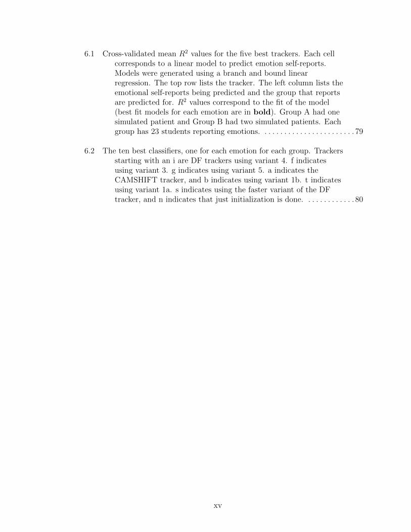
6.1 Cross-validated mean R2 values for the five best trackers. Each cellcorresponds to a linear model to predict emotion self-reports.Models were generated using a branch and bound linearregression. The top row lists the tracker. The left column lists theemotional self-reports being predicted and the group that reportsare predicted for. R2 values correspond to the fit of the model(best fit models for each emotion are in bold). Group A had onesimulated patient and Group B had two simulated patients. Eachgroup has 23 students reporting emotions. . . . . . . . . . . . . . . . . . . . . . . . 79
6.2 The ten best classifiers, one for each emotion for each group. Trackersstarting with an i are DF trackers using variant 4. f indicatesusing variant 3. g indicates using variant 5. a indicates theCAMSHIFT tracker, and b indicates using variant 1b. t indicatesusing variant 1a. s indicates using the faster variant of the DFtracker, and n indicates that just initialization is done. . . . . . . . . . . . . 80
xv
LIST OF FIGURES
Figure Page
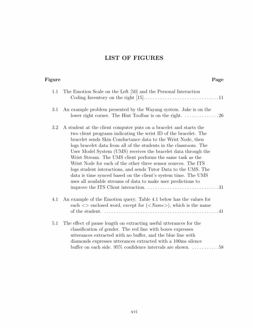
1.1 The Emotion Scale on the Left [50] and the Personal InteractionCoding Inventory on the right [15]. . . . . . . . . . . . . . . . . . . . . . . . . . . . . . . 11
3.1 An example problem presented by the Wayang system. Jake is on thelower right corner. The Hint Toolbar is on the right. . . . . . . . . . . . . . . 26
3.2 A student at the client computer puts on a bracelet and starts thetwo client programs indicating the wrist ID of the bracelet. Thebracelet sends Skin Conductance data to the Wrist Node, thenlogs bracelet data from all of the students in the classroom. TheUser Model System (UMS) receives the bracelet data through theWrist Stream. The UMS client performs the same task as theWrist Node for each of the other three sensor sources. The ITSlogs student interactions, and sends Tutor Data to the UMS. Thedata is time synced based on the client’s system time. The UMSuses all available streams of data to make user predictions toimprove the ITS Client interaction. . . . . . . . . . . . . . . . . . . . . . . . . . . . . . 31
4.1 An example of the Emotion query. Table 4.1 below has the values foreach <> enclosed word, except for (<Name>), which is the nameof the student. . . . . . . . . . . . . . . . . . . . . . . . . . . . . . . . . . . . . . . . . . . . . . . . 41
5.1 The effect of pause length on extracting useful utterances for theclassification of gender. The red line with boxes expressesutterances extracted with no buffer, and the blue line withdiamonds expresses utterances extracted with a 100ms silencebuffer on each side. 95% confidence intervals are shown. . . . . . . . . . . . 58
xvi

5.2 The effect of pause length on extracting useful utterances for the twoclass classification of culture (American vs. Asian). The leftshows the results for male subjects. The red line with boxesexpresses male utterances extracted with no buffer, the blue linewith diamonds expresses male utterances extracted with a 100mssilence buffer on each side. The right shows results for femalesubjects. The red line with down triangles expresses femaleutterances extracted with no buffer, the blue line with uptriangles expresses female utterances extracted with a 100mssilence buffer on each side. 95% confidence intervals are shown. . . . . . 59
6.1 Left: The key points for Group A with one simulated patient. Thekey points in this room were 1) The monitor, 2) the patient, and3) the telephone. In this frame, the student is closest to themonitor, but actually interacting with the patient. Right: Thekey points for Group B with two simulated patients. The keypoints in this room were 1) patient 1, 2) patient 2, and 3) thetelephone. In this frame the student is closest to patient 1. . . . . . . . . . 65
6.2 Two examples of the Reading People Tracker. Yellow rectanglesrepresent objects. Pink rectangles represent upper body. Redrectangles with a small inner rectangle represent heads. top:Multiple objects are found for one person, bottom: the foregrounddetection of the person begins to fade as the student stands verystill. . . . . . . . . . . . . . . . . . . . . . . . . . . . . . . . . . . . . . . . . . . . . . . . . . . . . . . . . 67
6.3 Two examples of the CAMSHIFT tracker. The blue box is the centerof the track, representing the head position. The red ellipse is thearea being tracked. top: the tracker center stays near the student,but the size of the track is most of the frame, bottom: the trackercenter goes to the wrong side of the patient. . . . . . . . . . . . . . . . . . . . . . . 68
6.4 An example of the Lucas-Kanade tracker. The head region is selectedby hand. As the student moves around the ‘good features totrack’ (in green) disperse away from the head. . . . . . . . . . . . . . . . . . . . . 69
6.5 Two examples of the distribution field tracker. Blue box representsthe area being tracked, in this case, the head of the student. top:tracker incorrectly selects filing cabinet, bottom: trackerincorrectly selects a box with dials . . . . . . . . . . . . . . . . . . . . . . . . . . . . . . 70
xvii

6.6 Left: Top ten trackers in order of increasing mean squared error.Right: Box plot of distances from ground truth for top tentrackers. Trackers beginning with ‘n’ use only initialization,trackers beginning with ‘a’ are variants of the CAMSHIFTtracker, and trackers beginning with ‘i’ are the DF trackers. . . . . . . . . 77
6.7 The predicted head positions of one student for two different trackers.Blue points predict closest to monitor. Green points predictclosest to patient, and Orange points predict student closest tothe telephone. Left: heuristic detection (no tracking). Right:distribution field tracker . . . . . . . . . . . . . . . . . . . . . . . . . . . . . . . . . . . . . . . 78
6.8 The PICI features that are common between groups A and B. . . . . . . . . 80
xviii

CHAPTER 1
INTRODUCTION
One of the strongest links between the way computers work and the way people
think was defined by the field of cognitive psychology [3], specifically the information
processing approach to cognitive psychology. The information processing approach
considers that the essence of the mind is processing the information available to peo-
ple in their environment. While computers use ones and zeros to process, people have
visual, audio, touch, smell, taste, and balance stimuli. In addition, these stimuli from
the environment are translated from physical signals to electrical signals and then
processed by the brain. According the information processing approach of cognitive
psychology, the mind takes in this sensory information, processes it based on a set of
rules, and comes up with answers, or decisions. In essence, this information process-
ing approach uses a computer paradigm to describe human cognition. Many great
advances in psychology came from this approach, including a learning mechanism
for computation called the neural network [80, 104]. Information processing is not
traditionally concerned with emotion; however, Herb Simon expressed that emotion
plays an important role in cognition, and that information processing theories should
include an “intimate association of cognitive processes with emotions and feelings”
[117]. This proclamation was made in 1967 as a response to Neisser’s article with the
headline “The view that machines will think as man does reveals misunderstanding of
the nature of human thought” [89]. However, only recently have researchers seriously
considered including emotion as an integral part of the architecture [12, 13, 28, 60].
1
The use of sensors to detect emotion has been attempted with varying levels of
success for many years.
In this chapter I discuss why the study of affect is important for the field of
computer science, and how affect is currently studied in general, and in the case of
humans interacting with computational systems.
1.1 Why Study Affect
Emotional intelligence is a clear factor in education [37, 73, 74], health care [90],
and day to day interaction [49]. In education, Wigfield and Karpathian found that low
motivation indicates less learning [132]. For health, there is evidence that a positive
emotional state can speed up recovery [90]. In addition, the onset, progression and
improvement of health and disease processes have been noted to impact the human
voice and produce unique changes in acoustic signals [124]. For personal interaction
there is evidence that individuals self-modulate their mood in anticipation of inter-
acting with another person [49]. In addition, nurses do ‘emotion work,’ modulating
their expression, to better care for patients [84]. But this evidence alone, may not be
enough to warrant studying affect for the purposes of computation.
Computer use in educational settings has been increasing rapidly since 1993 [119].
In 2003, 83.5% of students age 3 and above used computers in school up from 59% in
1993. In addition 47.2% of students age 3 and above in 2003 used computers at home
to do school work up from 14.8% in 1993. With this increase in use of computers
for educational purposes, and the link between understanding affect of students and
their performance, there is a clear need for computers to begin to understand the
emotions of students.
The study of affect for health purposes has been a research area for many years.
However, more recently there has been more of a push toward quantitative measures
of emotion, and these quantitative measures are an obvious place for computational
2
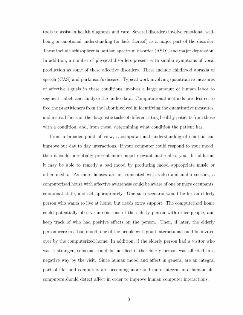
tools to assist in health diagnosis and care. Several disorders involve emotional well-
being or emotional understanding (or lack thereof) as a major part of the disorder.
These include schizophrenia, autism spectrum disorder (ASD), and major depression.
In addition, a number of physical disorders present with similar symptoms of vocal
production as some of these affective disorders. These include childhood apraxia of
speech (CAS) and parkinson’s disease. Typical work involving quantitative measures
of affective signals in these conditions involves a large amount of human labor to
segment, label, and analyze the audio data. Computational methods are desired to
free the practitioners from the labor involved in identifying the quantitative measures,
and instead focus on the diagnostic tasks of differentiating healthy patients from those
with a condition, and, from those, determining what condition the patient has.
From a broader point of view, a computational understanding of emotion can
improve our day to day interactions. If your computer could respond to your mood,
then it could potentially present more mood relevant material to you. In addition,
it may be able to remedy a bad mood by producing mood–appropriate music or
other media. As more houses are instrumented with video and audio sensors, a
computerized house with affective awareness could be aware of one or more occupants’
emotional state, and act appropriately. One such scenario would be for an elderly
person who wants to live at home, but needs extra support. The computerized home
could potentially observe interactions of the elderly person with other people, and
keep track of who had positive effects on the person. Then, if later, the elderly
person were in a bad mood, one of the people with good interactions could be invited
over by the computerized home. In addition, if the elderly person had a visitor who
was a stranger, someone could be notified if the elderly person was affected in a
negative way by the visit. Since human mood and affect in general are an integral
part of life, and computers are becoming more and more integral into human life,
computers should detect affect in order to improve human computer interactions.
3

1.2 The Study of Affect
In order to make the study of affect useful for computers, we need a quantitative
description of affect. The use of electronic sensors for affect detection allows for quan-
titative measure, however there is not yet agreement within the research community
on the best way, or the “gold standard,” for validating these quantitative measures.
Even without a “gold standard,” the method for quantitative measure is similar to
that of the scientific method of physical phenomena. The main difference is that
repeatability is more difficult due to inability to have purely controlled experiments,
and due to the fact that the nature of the object of experiment, namely the human,
is often changed by the experience of the experiment. This leads to empirical results
that can yield significant statistical results but do not give too much insight on an
individual event involving an individual person. This section will discuss 1) the affec-
tive channels that are available and methods for labeling them, 2) how computational
classification of affect can be performed given these channels and labels, and 3) the
target applications for the current body of work.
1.2.1 Affective Channels and Labels
People express emotions in many ways. Wilhelm Wundt described gesture com-
munication as originating from “emotion and the involuntary expressive movements
that accompany emotion” [135]. Wundt elaborated that actions in the face and the
body can be used to determine emotion, and that gestural communication with emo-
tion is able to elicit a similar emotion in the recipient of the communication. The
knowledge that humans involuntarily display their emotion, and that this display can
be observed and detected, is the basis for studying affect through observation and
sensors. Contemporary work utilizes four different channels for affect, namely faces,
voices, physiology and movement. Wang et al., [130] have used computational facial
expression analysis for understanding emotion impairments in schizophrenia. Busso
4

et al., [20] use features of fundamental frequency in voice to determine basic emotions
in speech. Mandryk and Atkins [77] used physiological data such as Galvanic Skin
Response (GSR), cardiovascular, and electro-myogram (EMG) data to detect emo-
tion of people playing a video game. Camurri et al., [23] created a gesture analysis
tool for looking at emotional expression in music and performance called EyesWeb.
The next few paragraphs discuss more detail of how faces, voices, physiology, and
movement have been used to study affect. Each channel has a variety of features
to choose from, and a variety of methods to label and categorize emotion. Several
research issues remain to be answered. What defines the ground truth emotion? Is
self-report accurate? Are quantitative metrics accurate and sensitive to note dif-
ferences in humans with respect to affect, cultural, and linguistic differences? Is
consistency of labeling indicative of quality? How important is the context of the
experience in determining the emotional state of the participant? Each of these ques-
tions are addressed differently by each work discussed below. Hopefully some clarity
will be gained by looking at these different approaches.
1.2.1.1 Faces
One early set of studies of facial expression involves the elicitation of various facial
expressions through electrophysiological stimulation of facial muscles by Guillaume-
Benjamin Duchenne [42, 43]. Duchenne found that some muscles have a complete
control over particular expressions, while other muscles have partial control over the
same expressions. Duchenne performed experiments by external manipulation, while
the computer allows modern researchers to do observational experiments, in which
the computer collects quantitative measurements of how facial expressions are made
during a particular affective state or activity. Charles Darwin drew analogies be-
tween animal and human expression as a continuing argument that man evolved from
a “lower animal form” [36]. In his work he dedicates eight chapters to “special ex-
5

pressions of man.” These include suffering and weeping, anxiety and despair, joy and
love, reflection and ill-temper (frowning), hatred and anger, contempt and disgust,
surprise and fear, and finally shame and modesty.
From this set of emotions, Paul Ekman empirically determined which of these
emotions were universally observed [44, 45]. That is, which of these emotions would
be recognized when viewing a still image of a person expressing the target emotion.
From this, Ekman found six universal emotions anger, joy, fear, disgust, surprise,
and sadness [44, 45]. In addition, this work brought about the facial action coding
system (FACS), which specifies particular visually observable motions in the face that
make up emotional expression. The FACS is the basis for much of the computational
detection of emotional expression in faces [33, 137].
In our intelligent tutoring system, we use a facial feature tracker that uses FACS-
like features to detect interpersonal mental states such as agreeing, disagreeing, un-
sure, thinking, concentrating, and interested [47].
1.2.1.2 Voices
Computational voice processing started in 1928 with Dudley’s vocoder (VOice
CODER) [111], which digitizes and synthesizes voice. The vocoder was designed as a
method for efficient electronic transmission of speech for Bell Telephone Laboratories.
Some uses of vocoders are for the encryption of voice, for blind people to listen to
recorded books at a fast rate, and to help partially deaf people hear speech better.
The technology for the vocoder evolved into many signal analysis tools specific to
voice processing. The sound spectrograph [68] was the first device for producing
visual printouts of speech called spectrograms. Before this, oscillographs were used
for detecting patterns in speech related to emotion [118]. Voice analysis is concerned
with vocal differences and quality.
6
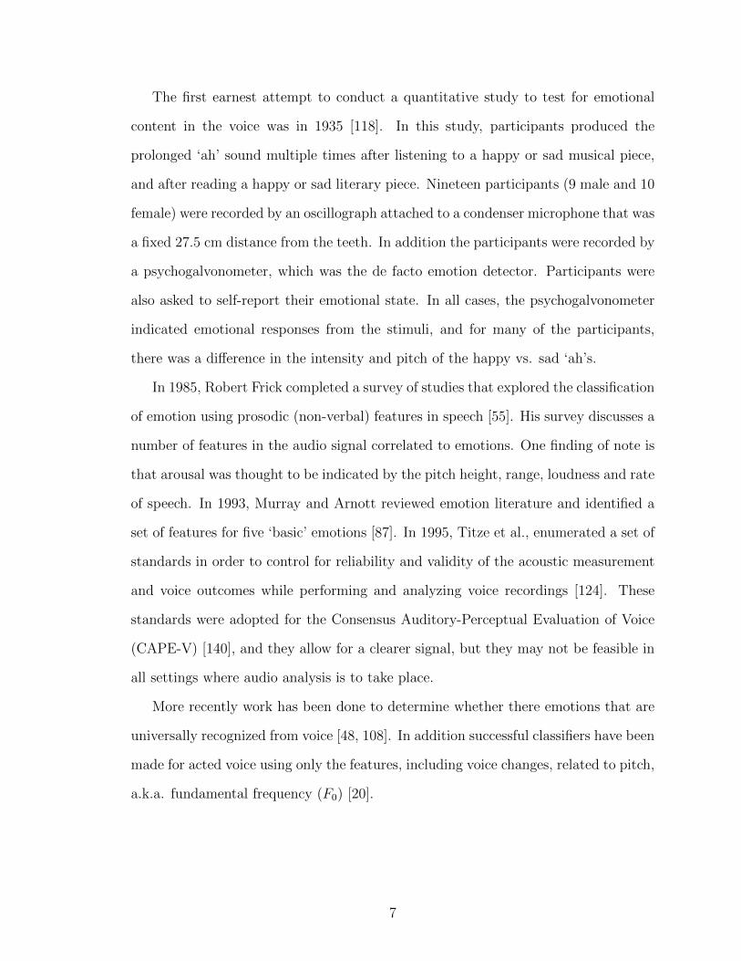
The first earnest attempt to conduct a quantitative study to test for emotional
content in the voice was in 1935 [118]. In this study, participants produced the
prolonged ‘ah’ sound multiple times after listening to a happy or sad musical piece,
and after reading a happy or sad literary piece. Nineteen participants (9 male and 10
female) were recorded by an oscillograph attached to a condenser microphone that was
a fixed 27.5 cm distance from the teeth. In addition the participants were recorded by
a psychogalvonometer, which was the de facto emotion detector. Participants were
also asked to self-report their emotional state. In all cases, the psychogalvonometer
indicated emotional responses from the stimuli, and for many of the participants,
there was a difference in the intensity and pitch of the happy vs. sad ‘ah’s.
In 1985, Robert Frick completed a survey of studies that explored the classification
of emotion using prosodic (non-verbal) features in speech [55]. His survey discusses a
number of features in the audio signal correlated to emotions. One finding of note is
that arousal was thought to be indicated by the pitch height, range, loudness and rate
of speech. In 1993, Murray and Arnott reviewed emotion literature and identified a
set of features for five ‘basic’ emotions [87]. In 1995, Titze et al., enumerated a set of
standards in order to control for reliability and validity of the acoustic measurement
and voice outcomes while performing and analyzing voice recordings [124]. These
standards were adopted for the Consensus Auditory-Perceptual Evaluation of Voice
(CAPE-V) [140], and they allow for a clearer signal, but they may not be feasible in
all settings where audio analysis is to take place.
More recently work has been done to determine whether there emotions that are
universally recognized from voice [48, 108]. In addition successful classifiers have been
made for acted voice using only the features, including voice changes, related to pitch,
a.k.a. fundamental frequency (F0) [20].
7
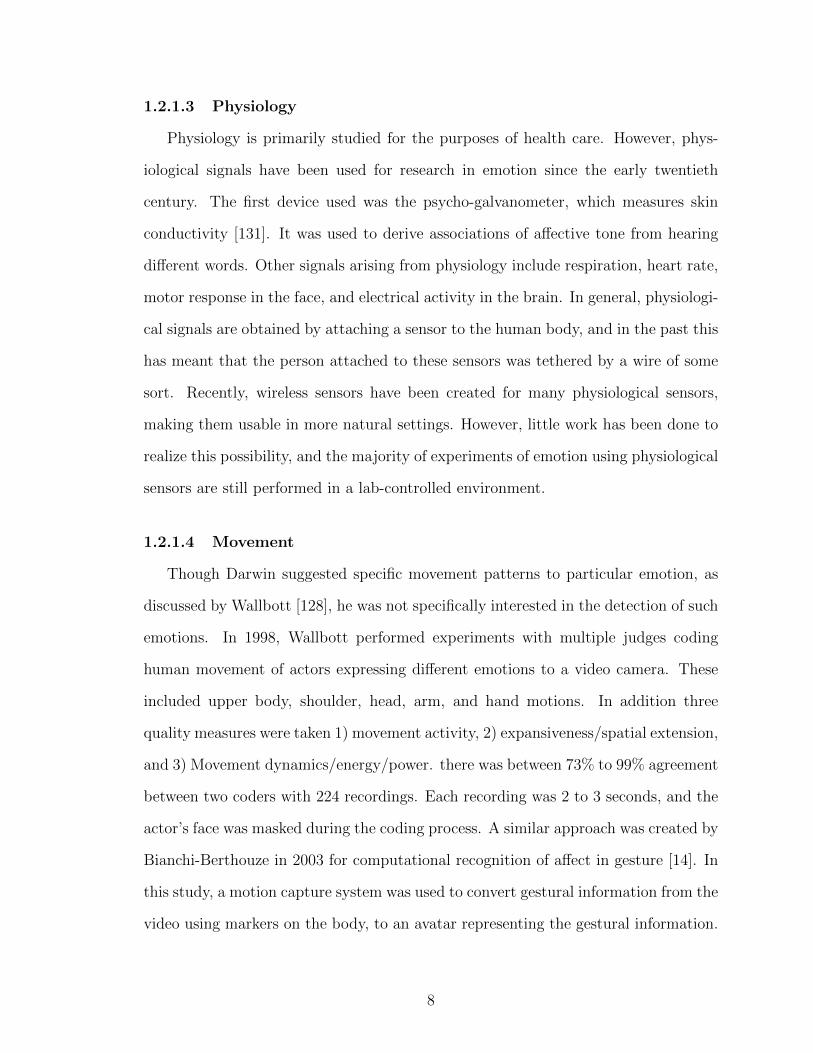
1.2.1.3 Physiology
Physiology is primarily studied for the purposes of health care. However, phys-
iological signals have been used for research in emotion since the early twentieth
century. The first device used was the psycho-galvanometer, which measures skin
conductivity [131]. It was used to derive associations of affective tone from hearing
different words. Other signals arising from physiology include respiration, heart rate,
motor response in the face, and electrical activity in the brain. In general, physiologi-
cal signals are obtained by attaching a sensor to the human body, and in the past this
has meant that the person attached to these sensors was tethered by a wire of some
sort. Recently, wireless sensors have been created for many physiological sensors,
making them usable in more natural settings. However, little work has been done to
realize this possibility, and the majority of experiments of emotion using physiological
sensors are still performed in a lab-controlled environment.
1.2.1.4 Movement
Though Darwin suggested specific movement patterns to particular emotion, as
discussed by Wallbott [128], he was not specifically interested in the detection of such
emotions. In 1998, Wallbott performed experiments with multiple judges coding
human movement of actors expressing different emotions to a video camera. These
included upper body, shoulder, head, arm, and hand motions. In addition three
quality measures were taken 1) movement activity, 2) expansiveness/spatial extension,
and 3) Movement dynamics/energy/power. there was between 73% to 99% agreement
between two coders with 224 recordings. Each recording was 2 to 3 seconds, and the
actor’s face was masked during the coding process. A similar approach was created by
Bianchi-Berthouze in 2003 for computational recognition of affect in gesture [14]. In
this study, a motion capture system was used to convert gestural information from the
video using markers on the body, to an avatar representing the gestural information.
8

The frame of the avatar with the moment of extreme expression of the emotion was
hand selected and labeled by a majority vote of 114 judges. These hand selected,
frontal view frames were used in a neural network called CALM to categorize the
avatar gestures as emotions. The CALM system got an average of 94% accuracy on
the training set, and was able to keep it’s accuracy above 70% with up to 5% random
noise added to the training data as a test set.
In 1999, Camurri et al., began the creation of a system for the computational
analysis of emotion in dance performances [22]. They used Rudolph Laban’s “Effort
Theory” to attempt to computationally capture four features of effort in dance: space,
time, weight, and flow. This resulted in a video based system called EyesWeb [23],
which extracts the silhouette of a person and measures a set of effort based features
that can be related to the emotion of the dancer. Further work was done by Castellano
et al., using the EyesWeb system where acted emotion was detected on the valence-
arousal axes based on front facing actors and their arm movements [25]. The EyesWeb
tool is designed to be interactive with a human user, and so it could not be used for
the purposes of the studies in this work.
Detecting emotion of a person interacting with the environment while not specifi-
cally facing the single camera in the room is a novel contribution. The work presented
here is a first step towards this goal, and there is a large potential for refinement by
using some of the more specific features found by the above mentioned research.
1.2.2 Affect Classification
Researchers have categorized the observation of emotion in a number of ways.
The two most prevalent are 1) a two-dimensional feature space, and 2) a discrete set
of classes for emotion.
Many words can be used to describe a person’s emotion; however, there is a need
to limit the number of emotional dimensions used for computation. This can be done
9
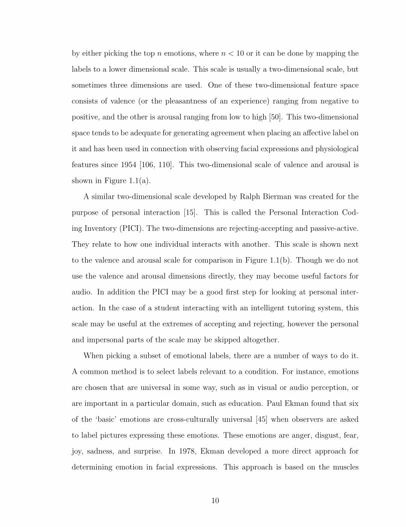
by either picking the top n emotions, where n < 10 or it can be done by mapping the
labels to a lower dimensional scale. This scale is usually a two-dimensional scale, but
sometimes three dimensions are used. One of these two-dimensional feature space
consists of valence (or the pleasantness of an experience) ranging from negative to
positive, and the other is arousal ranging from low to high [50]. This two-dimensional
space tends to be adequate for generating agreement when placing an affective label on
it and has been used in connection with observing facial expressions and physiological
features since 1954 [106, 110]. This two-dimensional scale of valence and arousal is
shown in Figure 1.1(a).
A similar two-dimensional scale developed by Ralph Bierman was created for the
purpose of personal interaction [15]. This is called the Personal Interaction Cod-
ing Inventory (PICI). The two-dimensions are rejecting-accepting and passive-active.
They relate to how one individual interacts with another. This scale is shown next
to the valence and arousal scale for comparison in Figure 1.1(b). Though we do not
use the valence and arousal dimensions directly, they may become useful factors for
audio. In addition the PICI may be a good first step for looking at personal inter-
action. In the case of a student interacting with an intelligent tutoring system, this
scale may be useful at the extremes of accepting and rejecting, however the personal
and impersonal parts of the scale may be skipped altogether.
When picking a subset of emotional labels, there are a number of ways to do it.
A common method is to select labels relevant to a condition. For instance, emotions
are chosen that are universal in some way, such as in visual or audio perception, or
are important in a particular domain, such as education. Paul Ekman found that six
of the ‘basic’ emotions are cross-culturally universal [45] when observers are asked
to label pictures expressing these emotions. These emotions are anger, disgust, fear,
joy, sadness, and surprise. In 1978, Ekman developed a more direct approach for
determining emotion in facial expressions. This approach is based on the muscles
10
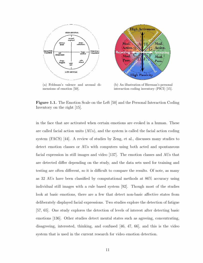
(a) Feldman’s valence and arousal di-mensions of emotion [50].
(b) An illustration of Bierman’s personalinteraction coding inventory (PICI) [15].
Figure 1.1. The Emotion Scale on the Left [50] and the Personal Interaction CodingInventory on the right [15].
in the face that are activated when certain emotions are evoked in a human. These
are called facial action units (AUs), and the system is called the facial action coding
system (FACS) [44]. A review of studies by Zeng, et al., discusses many studies to
detect emotion classes or AUs with computers using both acted and spontaneous
facial expression in still images and video [137]. The emotion classes and AUs that
are detected differ depending on the study, and the data sets used for training and
testing are often different, so it is difficult to compare the results. Of note, as many
as 32 AUs have been classified by computational methods at 86% accuracy using
individual still images with a rule based system [92]. Though most of the studies
look at basic emotions, there are a few that detect non-basic affective states from
deliberately displayed facial expressions. Two studies explore the detection of fatigue
[57, 65]. One study explores the detection of levels of interest after detecting basic
emotions [136]. Other studies detect mental states such as agreeing, concentrating,
disagreeing, interested, thinking, and confused [46, 47, 66], and this is the video
system that is used in the current research for video emotion detection.
11

In addition to facial expressions, work has been done to find cross-culturally uni-
versal emotions detectable by listening to voices [108]. Scherer found five emotional
states detectable in the voice. These are anger, fear, joy, neutral, and sadness.
A number of emotional labels are used in computer based education, including
frustration, fear/anxiety, shame/embarrassment, enthusiasm/excitement and pride
[91]; joy, distress, admiration, and reproach [30]; boredom, confusion, flow, frustra-
tion, and neutral [40]; and confident, excited, frustrated, and interested [8]. One goal
of these features is to label points where a computer tutoring system can modify its
interaction with the user. The interaction can change by modifying the task, offering
emotional support, offering cognitive support, or changing the presentation of the
task.
1.2.3 Target Applications
We explore three target applications of affect detection 1) computer based educa-
tion, 2) speaker differences on the basis of gender, culture/race and health diagnosis,
and 3) health care education. Specifically we use multiple sensors to explore the ef-
ficacy of detecting the affective state of students using an intelligent tutoring system
(ITS) in a classroom environment. We extract affective features of audio recordings
of clinical interviews in order to automatically classify gender and culture of patients.
We extract movement features from video recordings of nurses in training while taking
a practical examination in order to classify their emotions from the test.
1.3 Contributions
There are five contributions in this dissertation.
1. We show that affective learning states can be computationally determined in
both computer-based and health care education.
12
2. We show empirical evidence that the affective features of voice are useful for
the computational classification of gender, culture, and race.
3. We propose a novel method to track the head of a single person. This method
illuminates key problems that need to be solved in computer vision for the long
term real-time tracking of people.
4. We create a novel method to use video data to successfully classify self-reported
emotions in clinical simulation evaluation environments.
5. We show two examples of the successful use of sensors for research outside of
the laboratory.
1.4 Thesis Outline
This dissertation is organized as follows. This chapter introduced the problem of
detecting emotion for education and health care and described the scope of this work.
Chapter 2 gives a background to the sensors used for affect detection, and the methods
of classification for the prediction of affect. Chapter 3 discusses the use of affective
sensors in a classroom environment with Wayang Outpost, an intelligent tutoring
system (ITS) that teaches mathematics. The following hypotheses are explored: 1)
Sensors can effectively augment tutor logs in order to predict the self-reported emo-
tions of students. 2) Linear least squares classifiers built from the tutor and sensor
data can predict high vs. low levels of frustration, confidence, interest, and excite-
ment. Chapter 4 continues the computer based education study by exploring how
well the classifiers trained in Chapter 3 work with a separate larger population. One
hypothesis is explored from different perspectives: The accuracy, specificity, and/or
sensitivity of the frustration, confidence, interest, and excitement classifiers that use
tutor and/or sensor features will continue to perform significantly better than the
baseline classifier for the given emotion on a novel population. Chapter 5 introduces
13

the challenges of health diagnosis as well as identifying speaker differences using voice
features related to the emotional expression of speech. We explore data set of healthy
participants from different cultures and races to extract affective voice features for
the purpose of classifying gender, culture, and race. This chapter addresses the hy-
pothesis that the method of feature selection and linear least squares classification
will transfer to the voice domain. Chapter 6 discusses a novel application for com-
putational affect detection and classification. The goal of the system is to accurately
detect the self-reported emotion of a student nurse from the video and audio record-
ings of a practical clinical simulation evaluation in order to help the instructor identify
students who are likely to leave the program without intervention. The hypotheses
of this chapter are: 1) Low confidence is correlated with high anxiety in learning sit-
uations. 2) Available methods for real-time people tracking are adequate for tracking
the nurses in the video. 3) PICI related features in the video will help to predict or
classify the self-reported emotional state of the student. 4) Contemporary methods
for automatic extraction of audio will be sufficient to separate the student nurses
voice from other sounds and voices in the audio recording. 5) Prosodic features will
be relevant for emotional change. Chapter 7 concludes with a discussion of the re-
sults and limitations of this research in addition to future directions for research in
computational affect detection for education and health.
14

CHAPTER 2
BACKGROUND
2.1 Affective Sensors
2.1.1 Education Use
The four sensors used in the current Computer Based Education study are similar
to sensors that have been used in previous studies done by the Affective Computing
Group (ACG) at MIT. However, Arizona State University (ASU) invested consid-
erable effort to decrease the overall production cost and improve the non-invasive
nature of the sensors. We compare the ASU sensors to their predecessors as well as
some of the past uses of such sensors.
2.1.1.1 Skin Conductance Bracelet
The current research employs the next generation of HandWave electronics [121],
providing greater reliability, lower power requirements through wireless RFID trans-
mission and a smaller form. This smaller form was redesigned to minimize the visual
impact and increase the wearable aspects of previous versions. ASU integrated and
tested these electronic components into a wearable package suitable for students in
classrooms. This version reports at 1Hz. The bracelet sensor prototype parts came
at a discounted price of $150, with 3 hours of assembly time, and the radio to com-
municate with the sensors for the classroom costs $200.
2.1.1.2 Pressure Sensitive Mouse
ACG developed the pressure sensitive mouse [97]. It uses six pressure sensors
embedded in the surface of the mouse to detect the tension in a user’s grip and it
15

has been used to infer elements of a user’s frustration level. Our endeavors replicated
ACG’s pressure sensitive mouse and produced 30 units to be used in a classroom.
The new design of the mouse minimized the changes made to the physical appear-
ances of the original mouse in order to maintain a visually non-invasive sensor, while
maintaining functionality. The parts for the mouse cost $200 plus 3 hours of assembly.
2.1.1.3 Pressure Sensitive Chair
The chair sensor system was developed at ASU using a series of six force sensitive
resistors as pressure sensors dispersed strategically in the seat and back of a readily
available seat cover cushion. It is a greatly simplified version of the Tek-Scan Pressure
system (costing around $10,000) used in research by ACG [19, 66]. This posture chair
sensor was developed at ASU at an approximate material cost of $200 plus 2 hours
of labor for assembly and testing per chair for a production volume of 30 chairs.
2.1.1.4 Mental State Camera
The studies by ACG [19, 66] utilized IBM Research’s Blue-Eyes camera hardware.
This is special purpose hardware for facial feature detection. In our current research
we use a standard $50 web-camera to obtain 30 fps at 320x240 pixels. The camera
is placed on the monitor of each student’s computer. This is coupled with the Min-
dReader library from el Kaliouby [47] using a Java Native Interface (JNI) wrapper
developed at UMass. The interface starts a version of the MindReader software, and
can be queried at any time to acquire the most recent mental state values that have
been computed by the library. In the version used in the current experiments, we use
the six mental state features (agreeing, disagreeing, concentrating, interested, think-
ing, and unsure), but not the facial feature point or action unit detections. The six
mental features have a 65% to 89% accuracy with five out of the six features reported
at above 76% accuracy when compared to the ground truth acted expression data
16
[47]. The MindReader software is under license from MIT, and it uses a facial feature
tracker licensed by Google.
2.1.2 Voice Sensors
2.1.2.1 Voice in Health
During a clinical psychological interview, many different rating systems are used
to classify affective disorders. For example, to identify schizophrenia, clinicians use
instruments such as the Scale for the Assessment of Negative Symptoms (SANS) [4].
Many of the symptoms the clinician must identify have to do with how the person
speaks, including affective flattening, blunted affect, the inability to experience or
express a normal range of affective responses, emotional dullness, pervasive apathy,
poverty of speech and psycho-motor retardation [120]. Since these symptoms are
indicative of schizophrenia and can be detected by our ears, some researchers have
found the corresponding speech signals that can be processed by a computer [4, 120].
Diagnosing depressed patients has a similar set of rating instruments. For exam-
ple, reduced speech flow and prosody are both indicative of depression during free
speech tasks, though not as much during reading tasks. In addition, acoustic features
are more discriminating depending on whether the depressed person is categorized
as having psycho-motor agitation or psycho-motor retardation [2]. A computer sys-
tem has been created to semi-automatically distinguish between a highly depressive
tendency and a mildly depressive tendency [123]. The features utilized only included
pitch, amplitude range and utterance speed.
2.1.2.2 Voice in Emotion
Busso et al., recently found that the fundamental frequency and it’s derivative can
each be broken down into fourteen statistics, eleven of which can be used for sentence
level processing, and eleven of which can be used as a voiced level statistic. These
features can be used in a logistic regression classifier to predict levels of different
17
emotions such as anger, happiness and sadness using 3 different emotional databases.
Accuracies between 73% and 98% were attained where the baselines were between
54% and 89%. There was no ranking to see if the classifier was significantly better
than the baseline, however a large number of the emotion classifiers have R2 values
above 0.63.
2.1.2.3 Voice in Culture
Walton and Orlikoff tested the ability of people to recognize differences between
race solely on voice was tested in the distinguishing between white and black American
voices [129]. Twelve judges, six experienced speech pathologists and six inexperienced
speech pathology students were able to detect race with 60% accuracy. Since the mean
pitch, first and second formant frequencies were not distinguishable between groups,
the authors concluded that people must use spectral information and not pitch infor-
mation to distinguish between race. Ryalls et al., found that voice onset times (VOT)
for specific vowels and consonants were significantly different between Caucasian and
African American subjects [107]. They also found significant differences of VOT for
gender.
Andrianopoulos et al., [5, 6] identified significant differences between healthy
speakers on the basis age, gender, culture and race by teasing-out subtle and salient
features of the acoustic signal that differentiated four different cultural and racial
groups of speakers. As predicted, male speakers voices regardless of culture and race
were significantly lower in pitch compared to their female counterparts. Moreover,
Mandarin Chinese and Hindi Indian males and females prolonged the three univer-
sal vowels, [a], [i] and [u], with significantly higher pitch voices compared to their
Caucasian and African American male and female counterparts. Males regardless of
culture and race exhibited significantly greater frequency and amplitude perturbation
compared to their female counterparts. More recently, the subtle and salient differ-
18
ences in speakers with neurodevelopmental programs, such as an Autism Spectrum
Disorder (ASD), are being studies by these researchers. To date, these authors have
found similar trends in those individuals with ASD in that they speak with signifi-
cantly higher pitch voices, with fewer semitones and restricted pitch ranges. These
acoustic features noted in these populations support that individuals with ASD speak
with higher pitch voices with ‘monopitch’ and ‘monoloudness’ [127].
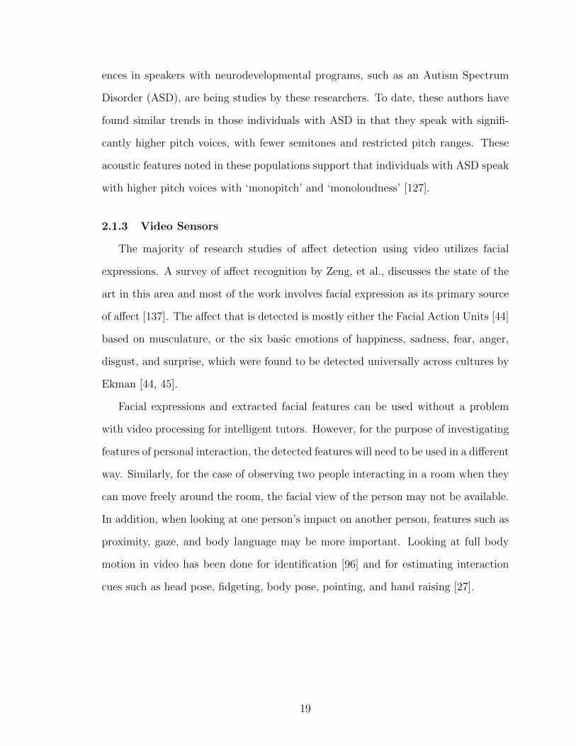
2.1.3 Video Sensors
The majority of research studies of affect detection using video utilizes facial
expressions. A survey of affect recognition by Zeng, et al., discusses the state of the
art in this area and most of the work involves facial expression as its primary source
of affect [137]. The affect that is detected is mostly either the Facial Action Units [44]
based on musculature, or the six basic emotions of happiness, sadness, fear, anger,
disgust, and surprise, which were found to be detected universally across cultures by
Ekman [44, 45].
Facial expressions and extracted facial features can be used without a problem
with video processing for intelligent tutors. However, for the purpose of investigating
features of personal interaction, the detected features will need to be used in a different
way. Similarly, for the case of observing two people interacting in a room when they
can move freely around the room, the facial view of the person may not be available.
In addition, when looking at one person’s impact on another person, features such as
proximity, gaze, and body language may be more important. Looking at full body
motion in video has been done for identification [96] and for estimating interaction
cues such as head pose, fidgeting, body pose, pointing, and hand raising [27].
19

2.2 Classification as Prediction
One goal of this dissertation is to use classification in order to predict the affective
state of a person. Prediction is possible since people express their emotions in ways
that are detectable by sensors. Simply put, a classifier takes as input a finite number
of features, and based on the value of these features decides into which category the
input fits. In the case of predicting emotion, this translates to taking sensor features
and deciding which emotion the person is displaying.
However, using classification as a method for prediction has a number of risks. 1.
Classifiers generally do not learn on the fly. 2. Individuals exhibit the same emotion
in many different ways. 3. The affective signal may become contaminated due to
ambient noise and other environmental factors. 4. Cues for emotion overlap with
cues for other expression such as communication and language.
2.2.1 Ideal Conditions
To date, the ideal conditions for classification are:
1. Large population size.
2. Large set of data.
3. Data sample evenly distributed over the population in question.
4. Balanced sample from classes.
5. Independent features.
6. Data drawn from independent and identically distributed (i.i.d.) or exchange-
able random variables
7. Implementation of control variables to increase reliability and validity of classi-
fications systems given the current state of the art in technology.
20
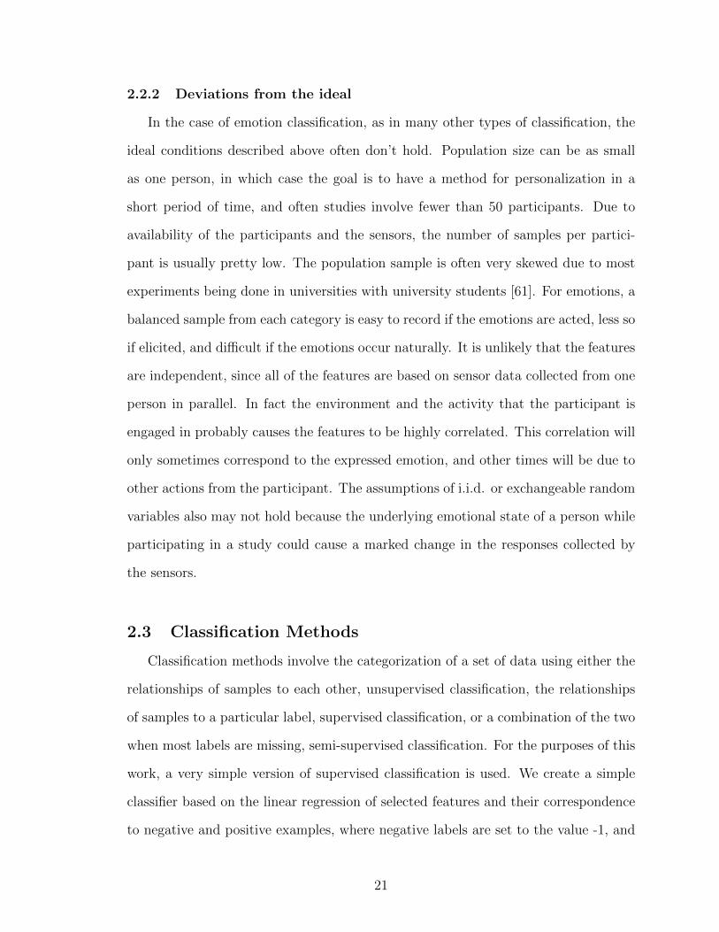
2.2.2 Deviations from the ideal
In the case of emotion classification, as in many other types of classification, the
ideal conditions described above often don’t hold. Population size can be as small
as one person, in which case the goal is to have a method for personalization in a
short period of time, and often studies involve fewer than 50 participants. Due to
availability of the participants and the sensors, the number of samples per partici-
pant is usually pretty low. The population sample is often very skewed due to most
experiments being done in universities with university students [61]. For emotions, a
balanced sample from each category is easy to record if the emotions are acted, less so
if elicited, and difficult if the emotions occur naturally. It is unlikely that the features
are independent, since all of the features are based on sensor data collected from one
person in parallel. In fact the environment and the activity that the participant is
engaged in probably causes the features to be highly correlated. This correlation will
only sometimes correspond to the expressed emotion, and other times will be due to
other actions from the participant. The assumptions of i.i.d. or exchangeable random
variables also may not hold because the underlying emotional state of a person while
participating in a study could cause a marked change in the responses collected by
the sensors.
2.3 Classification Methods
Classification methods involve the categorization of a set of data using either the
relationships of samples to each other, unsupervised classification, the relationships
of samples to a particular label, supervised classification, or a combination of the two
when most labels are missing, semi-supervised classification. For the purposes of this
work, a very simple version of supervised classification is used. We create a simple
classifier based on the linear regression of selected features and their correspondence
to negative and positive examples, where negative labels are set to the value -1, and
21

positive labels are set to the value 1. The classifier predicts based on a linear model,
and predictions above 0 are considered to be in the positive class, and in the negative
class if predicted otherwise. This simple method allows for very fast computation,
it requires very little memory, and it gives a starting point for how well the selected
features work together for classification.
The results from constructing a linear classifier, are by no means the final word on
how well particular features will work for classifying a set of labelled data, but they
do give an answer to the question of what are sufficient features for classifying a set
of labelled data. Since the focus of this work is on feasibility of computational affect
detection for education and heath care applications, the first step is to find a method
that works. Then that method can be built upon with more advanced computational
techniques in future work.
22
CHAPTER 3
USER MODEL FOR COMPUTER BASED EDUCATION
Traditionally, the user model of an intelligent tutoring system (ITS) consists of
registration information with or without statistics about interactions with the ITS
[67, 115]. Registration information often includes age, gender, class standing, teacher,
other static information about learners, and sometimes includes cultural and racial
make-up. A limitation of this approach is that the only dynamic information that the
ITS uses is based on the cognitive performance of the students. With the use of non-
invasive sensors, we have the opportunity to enhance user models with sensor data
that is a natural byproduct of the student’s interaction with the ITS. Though the cost
of such sensors has previously made them less accessible for classroom deployment,
recent strides have been made to address this limitation. Arizona State University
(ASU), in collaboration with the Affective Computing Group (ACG) at MIT, has
developed 30 lower-cost versions of four sensors that have shown promise for their
ability to detect elements of students’ emotional expression. These sensors described
in Section 2.1.1 include a pressure sensitive mouse, a pressure sensitive chair, a skin
conductance wristband, and a camera based facial expression recognition system that
incorporates a computational framework that aims to infer a user’s state of mind.
At UMass Amherst, we have built on ASU’s work by integrating the sensors and an
Emotional Query intervention module with a traditional ITS user interaction based
models to obtain the students’ reported emotions as they interact with the tutor.
This enables the user model system (UMS) to compare sensor readings at the time
of the emotional queries.
23
Ultimately we plan to have a UMS that models the student’s interaction with an
ITS in real-time and enables the ITS to intelligently tailor its behavior to a given
student’s needs. By personalizing the student’s experience, the ITS can keep the
student engaged and maintain or increase the student’s interest and confidence in the
subject. [10] is an example of having an animated character as part of the tutor giving
non-verbal feedback, [53] is an example of a tutor that changes its feedback based
on the character’s virtual emotional state in response to the student’s emotion. For
instance, a positive student emotional state elicits happiness in the character, which
in turn rewards the student. In order to create the desired UMS, we have developed
a platform comprised of three functional interacting components. These are (1) a
sensor system for processing and integrating the sensor data described in Sec. 3.2.2,
(2) a pedagogical engine for tutoring the student and collecting tutor data described
in Sec. 3.2.1, and (3) a user model system for integrating the sensor and tutor data to
create a model of the student. We conducted three experiments using this framework
in order to determine which sensor features have the best utility in terms of modeling
students’ perceived emotional state.
3.1 Related Work
There are a number of systems that already exist that either use similar sensors,
detect similar affective states, or incorporate both tutor data and sensor data in order
to model the student’s self reported emotion.
Zhou et al., uses a number of sensors to detect facial expressions, physiological
features (heart rate, temperature, and skin conductance), and speech signals [138].
The experiment uses 32 students simultaneously. This application measures emotional
responses elicited by the presentation of images rather than from using a tutor system.
The emotions that they model are fear, anger, and frustration.
24
McQuiggan et al., use a 3-D learning environment as their tutoring system. The
systems monitor heart-rate and skin conductance in addition to the student-tutor
interactions [82, 83]. They create a model of frustration [82] and self-efficacy [83],
i.e., the student’s belief in producing a correct answer.
Other work such as Florea and Kalisz, does not use sensors at all, but only uses
self reports to determine emotional state [53]. They use three emotional ranges to
model the student: boredom vs. curiosity, distress vs. enthusiasm, and anxiety vs.
confidence. With the model of the student, they then create a model of their tutor
to have emotional states that guide the tutor’s responses. The focus of this system is
the repair rather than the detection of emotional states.
Much of the past research has focused on small populations of students or lab
studies, while our research uses large groups of students in real school settings. This
is relevant because much research has shown that students lose interest and self-
confidence in math over the course of the K-12 school system [105, 26, 125]. Bringing
sensors to our children’s schools addresses real problems of students’ relationship
to mathematics as they learn the subject. This brings new tools to address their
frustration, anxiety and disinterest/boredom while learning.
3.2 Affect Detection System
3.2.1 The Tutor: Wayang Outpost
Our test-bed application for the experiments we describe in Sec. 3.3 was Wayang
Outpost, a multimedia Intelligent Tutoring System (ITS) for geometry [7]. The tu-
toring software is adaptive in that it iterates through different topic sections (e.g.
Pythagorean theorem). Within each topic section, Wayang adjusts the difficulty of
problems provided depending on past student performance. Students are presented
with a problem and asked to choose the solution from a list of multiple choice options
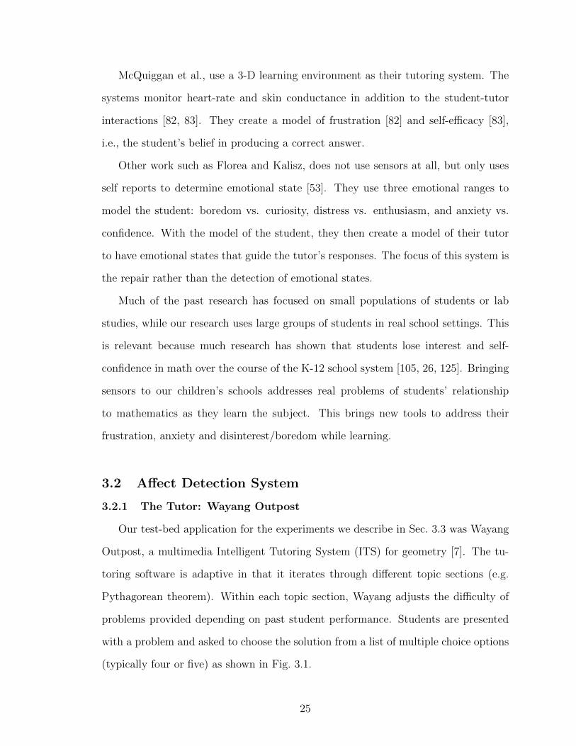
(typically four or five) as shown in Fig. 3.1.
25
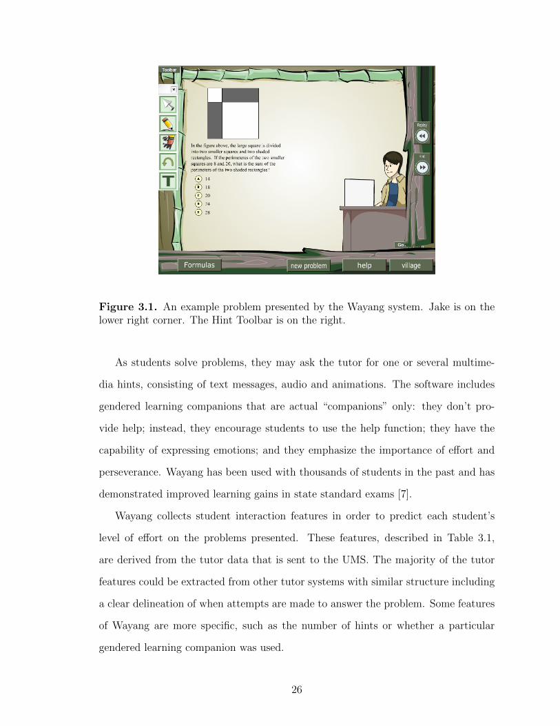
Figure 3.1. An example problem presented by the Wayang system. Jake is on thelower right corner. The Hint Toolbar is on the right.
As students solve problems, they may ask the tutor for one or several multime-
dia hints, consisting of text messages, audio and animations. The software includes
gendered learning companions that are actual “companions” only: they don’t pro-
vide help; instead, they encourage students to use the help function; they have the
capability of expressing emotions; and they emphasize the importance of effort and
perseverance. Wayang has been used with thousands of students in the past and has
demonstrated improved learning gains in state standard exams [7].
Wayang collects student interaction features in order to predict each student’s
level of effort on the problems presented. These features, described in Table 3.1,
are derived from the tutor data that is sent to the UMS. The majority of the tutor
features could be extracted from other tutor systems with similar structure including
a clear delineation of when attempts are made to answer the problem. Some features
of Wayang are more specific, such as the number of hints or whether a particular
gendered learning companion was used.
26
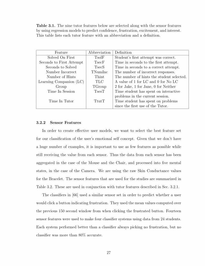
Table 3.1. The nine tutor features below are selected along with the sensor featuresby using regression models to predict confidence, frustration, excitement, and interest.This table lists each tutor feature with an abbreviation and a definition.
Feature Abbreviation DefinitionSolved On First TsolF Student’s first attempt was correct.
Seconds to First Attempt TsecF Time in seconds to the first attempt.Seconds to Solved TsecS Time in seconds to a correct attempt.Number Incorrect TNumInc The number of incorrect responses.Number of Hints Thint The number of hints the student selected.
Learning Companion (LC) TLC A value of 1 for LC and 0 for No LCGroup TGroup 2 for Jake, 1 for Jane, 0 for Neither
Time In Session TsesT Time student has spent on interactiveproblems in the current session.
Time In Tutor TtutT Time student has spent on problemssince the first use of the Tutor.
3.2.2 Sensor Features
In order to create effective user models, we want to select the best feature set
for our classification of the user’s emotional self concept. Given that we don’t have
a huge number of examples, it is important to use as few features as possible while
still receiving the value from each sensor. Thus the data from each sensor has been
aggregated in the case of the Mouse and the Chair, and processed into five mental
states, in the case of the Camera. We are using the raw Skin Conductance values
for the Bracelet. The sensor features that are used for the studies are summarized in
Table 3.2. These are used in conjunction with tutor features described in Sec. 3.2.1.
The classifiers in [66] used a similar sensor set in order to predict whether a user
would click a button indicating frustration. They used the mean values computed over
the previous 150 second window from when clicking the frustrated button. Fourteen
sensor features were used to make four classifier systems using data from 24 students.
Each system performed better than a classifier always picking no frustration, but no
classifier was more than 80% accurate.
27
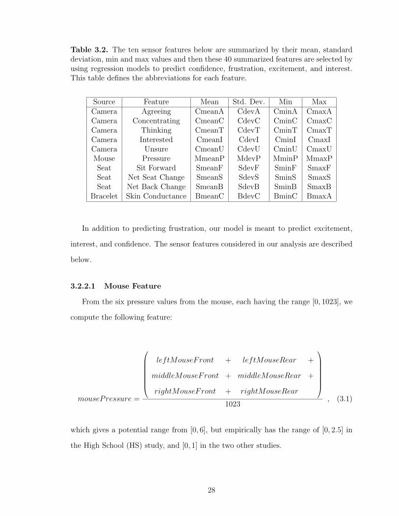
Table 3.2. The ten sensor features below are summarized by their mean, standarddeviation, min and max values and then these 40 summarized features are selected byusing regression models to predict confidence, frustration, excitement, and interest.This table defines the abbreviations for each feature.
Source Feature Mean Std. Dev. Min MaxCamera Agreeing CmeanA CdevA CminA CmaxACamera Concentrating CmeanC CdevC CminC CmaxCCamera Thinking CmeanT CdevT CminT CmaxTCamera Interested CmeanI CdevI CminI CmaxICamera Unsure CmeanU CdevU CminU CmaxUMouse Pressure MmeanP MdevP MminP MmaxPSeat Sit Forward SmeanF SdevF SminF SmaxFSeat Net Seat Change SmeanS SdevS SminS SmaxSSeat Net Back Change SmeanB SdevB SminB SmaxB
Bracelet Skin Conductance BmeanC BdevC BminC BmaxA
In addition to predicting frustration, our model is meant to predict excitement,
interest, and confidence. The sensor features considered in our analysis are described
below.
3.2.2.1 Mouse Feature
From the six pressure values from the mouse, each having the range [0, 1023], we
compute the following feature:
mousePressure =
leftMouseFront + leftMouseRear +
middleMouseFront + middleMouseRear +
rightMouseFront + rightMouseRear
1023
, (3.1)
which gives a potential range from [0, 6], but empirically has the range of [0, 2.5] in
the High School (HS) study, and [0, 1] in the two other studies.
28
3.2.2.2 Chair Features
We compute three features from the 6 chair sensors. The first two are based on
the most useful features from [38]. These are the net change in pressure of the seat,
and the net change in pressure of the back:
netSeatChange[t] =
∣∣∣∣∣∣∣∣∣∣∣∣
LeftSeat[t− 1] − leftSeat[t] +
MiddleSeat[t− 1] − middleSeat[t] +
RightSeat[t− 1] − rightSeat[t]
∣∣∣∣∣∣∣∣∣∣∣∣, (3.2)
netBackChange =
∣∣∣∣∣∣∣∣∣∣∣∣
lastLeftBack − leftBack +
lastMiddleBack − middleBack +
lastRightBack − rightBack
∣∣∣∣∣∣∣∣∣∣∣∣, (3.3)
The third chair feature is meant to determine if the student is sitting forward.
From the three pressure values from the back of the chair, each having the range
[0, 1023], we compute the Sit Forward feature as follows:
sitForward =
0 if leftBack > 200 or
middleBack > 200 or
rightBack > 200
1 if 200 >= leftBack > −1 and
200 >= middleBack > −1 and
200 >= rightBack > −1
NA otherwise
,
(3.4)
where NA is treated as no data.
29
3.2.2.3 Bracelet Feature
There are two values that we obtain from the wrist sensor, one is the battery
voltage to inform us when the battery charge is low, and the other is the skin conduc-
tance in Microsiemens. Since there was no need to reduce the number of features, we
processed basic statistics on the raw sensor values. In the future we plan to examine
more sophisticated use of the skin conductance data such as the methods used by
McQuiggan et al., [83].
3.2.2.4 Mental State Camera Features
Of the six mental state features that the MindReader software identifies, we com-
bine the agree and disagree states into one state about agreement, where the range
of [1.0,0.0] of the disagree state is translated to 0.0 to 0.5 of agreeing, and the agree-
ing state is translated to the 0.5 to 0.1 value of agreeing. The five features we are
left with are agreeing, concentrating, interested, thinking, and unsure. These mental
states have a range from [0, 1] as they are confidence values.
3.2.3 Feature Integration
In our framework, each feature source from each student is a separate stream of
data. Hence we have five streams of data that each report asynchronously and at
different rates. In order to merge all of the data sources, the wrist ID from each
student, and a time of the report was needed from each source. An example of one
client connected to our User Model Framework is shown in Fig. 3.2.
In our experiments, we used the student logs rather than the sensor streams, since
the streams are not yet informing a user model. In addition, the tutor does not yet
create a stream of tutor data. Instead we used a database query to obtain the relevant
tutor information, and fed it to the User Model System with the four sensor sources
in order to time align the data and merge it with the correct student. The result is
a database table with a row for every time stamp and wrist ID pair, and a column
30
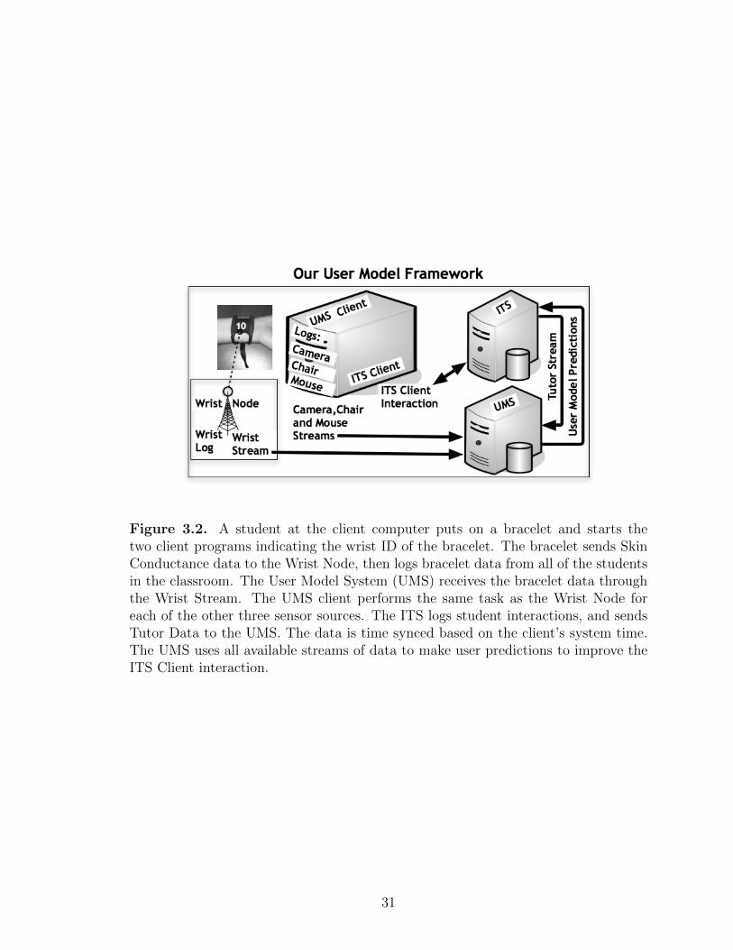
Figure 3.2. A student at the client computer puts on a bracelet and starts thetwo client programs indicating the wrist ID of the bracelet. The bracelet sends SkinConductance data to the Wrist Node, then logs bracelet data from all of the studentsin the classroom. The User Model System (UMS) receives the bracelet data throughthe Wrist Stream. The UMS client performs the same task as the Wrist Node foreach of the other three sensor sources. The ITS logs student interactions, and sendsTutor Data to the UMS. The data is time synced based on the client’s system time.The UMS uses all available streams of data to make user predictions to improve theITS Client interaction.
31
for each reported sensor value and tutor data value. Each cell in a row represents
the latest report of the data source. If the data source has never reported or has not
reported since the last tutor log in or log out event with a corresponding wrist ID,
then the value is -1 until the data source reports again. In this way the wrist IDs
can be used by more than one student at separate time intervals, and the system will
continue to work.
3.3 Experimental Setup
We conducted three studies during Fall 2008 using our sensor system with Wayang
Outpost. The HS study involved 35 students in a public high school in Massachusetts;
the UMASS study involved 29 students in the University of Massachusetts; the AZ
study involved 29 undergraduate students from Arizona State University. In the
HS and UMASS studies, students used the software as part of their regular math
class for 4-5 days, as it covered topics in the class. The AZ study was a lab study,
where students came to a lab in the university and used the software for one single
session. Wayang worked the same way for all students, as introduced in Sec. 3.2.1,
except for the fact that a student could be randomly assigned the female learning
companion (Jane), the male learning companion (Jake) or no learning companion.
In order to gather information on students’ emotions, Wayang prompted students to
report how they were feeling (e.g., “How [interested/excited/confident/frustrated] do
you feel right now?”). Students answered this prompt by choosing one item from
a five-point scale, where a three corresponded to a neutral value and the ends were
labeled with extreme values (e.g., “ I feel anxious/ very confident”). The queried
emotion was randomly chosen, obtaining a report per student per emotion for most
subjects. Wayang queried students on their emotions every five minutes, but did not
interrupt students as they were solving a problem. During each student’s interaction
32
with Wayang, the four sensors described in Sec. 2.1.1 gathered data on his or her
physiological responses.
3.4 Affect Classifiers
The three experiments yielded the results of 588 emotional queries from 80 stu-
dents that include valid data from at least one sensor. The queries were separated
into the four emotion variables as follows: 149 were about confidence/anxiety, 163
were about excitement/depression, 135 were about interest/boredom, and 141 were
about frustration/no frustration. 16 of the student responses gave no answer to the
emotional query. These results were used as examples for the regression and the
training and testing of the classification models.
In order to select a subset of the available features, a stepwise linear regression
was performed with each of the emotions as the dependent variable, and tutor and
sensor features as the independent variables. Since some students had missing sensor
data, separate models were run pairing the Tutor Features with Sensor Features from
one sensor at a time, and then finally with all of the Sensor Features. Results from
the regression in Table 3.4 show that the best models for confidence, frustration,
and excitement came from the subset of examples where all of the sensor data was
available, and the best model for interest came from the subset of examples with
mouse data available.
Table 3.4 shows the features selected for each of the linear models. The stepwise
linear least squares regression reduces the feature set to at most five of the available
features. In addition, only two of the four available sensors are used when creating
classifiers from all sensors with the tutor.
33
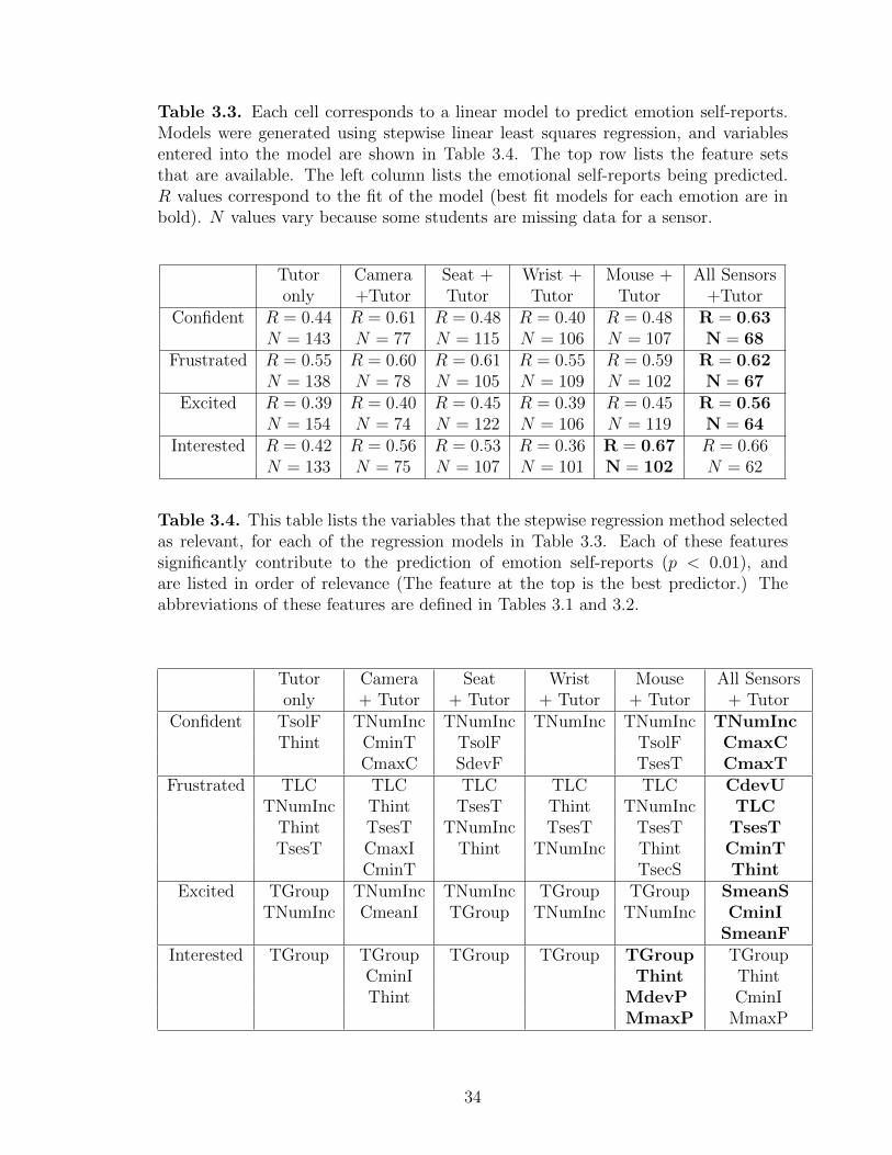
Table 3.3. Each cell corresponds to a linear model to predict emotion self-reports.Models were generated using stepwise linear least squares regression, and variablesentered into the model are shown in Table 3.4. The top row lists the feature setsthat are available. The left column lists the emotional self-reports being predicted.R values correspond to the fit of the model (best fit models for each emotion are inbold). N values vary because some students are missing data for a sensor.
Tutor Camera Seat + Wrist + Mouse + All Sensorsonly +Tutor Tutor Tutor Tutor +Tutor
Confident R = 0.44 R = 0.61 R = 0.48 R = 0.40 R = 0.48 R = 0.63N = 143 N = 77 N = 115 N = 106 N = 107 N = 68
Frustrated R = 0.55 R = 0.60 R = 0.61 R = 0.55 R = 0.59 R = 0.62N = 138 N = 78 N = 105 N = 109 N = 102 N = 67
Excited R = 0.39 R = 0.40 R = 0.45 R = 0.39 R = 0.45 R = 0.56N = 154 N = 74 N = 122 N = 106 N = 119 N = 64
Interested R = 0.42 R = 0.56 R = 0.53 R = 0.36 R = 0.67 R = 0.66N = 133 N = 75 N = 107 N = 101 N = 102 N = 62
Table 3.4. This table lists the variables that the stepwise regression method selectedas relevant, for each of the regression models in Table 3.3. Each of these featuressignificantly contribute to the prediction of emotion self-reports (p < 0.01), andare listed in order of relevance (The feature at the top is the best predictor.) Theabbreviations of these features are defined in Tables 3.1 and 3.2.
Tutor Camera Seat Wrist Mouse All Sensorsonly + Tutor + Tutor + Tutor + Tutor + Tutor
Confident TsolF TNumInc TNumInc TNumInc TNumInc TNumIncThint CminT TsolF TsolF CmaxC
CmaxC SdevF TsesT CmaxTFrustrated TLC TLC TLC TLC TLC CdevU
TNumInc Thint TsesT Thint TNumInc TLCThint TsesT TNumInc TsesT TsesT TsesTTsesT CmaxI Thint TNumInc Thint CminT
CminT TsecS ThintExcited TGroup TNumInc TNumInc TGroup TGroup SmeanS
TNumInc CmeanI TGroup TNumInc TNumInc CminISmeanF
Interested TGroup TGroup TGroup TGroup TGroup TGroupCminI Thint ThintThint MdevP CminI
MmaxP MmaxP
34
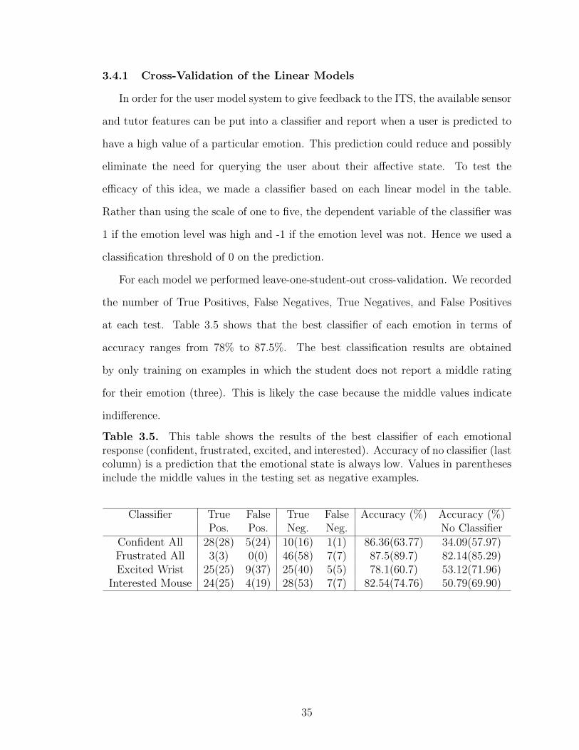
3.4.1 Cross-Validation of the Linear Models
In order for the user model system to give feedback to the ITS, the available sensor
and tutor features can be put into a classifier and report when a user is predicted to
have a high value of a particular emotion. This prediction could reduce and possibly
eliminate the need for querying the user about their affective state. To test the
efficacy of this idea, we made a classifier based on each linear model in the table.
Rather than using the scale of one to five, the dependent variable of the classifier was
1 if the emotion level was high and -1 if the emotion level was not. Hence we used a
classification threshold of 0 on the prediction.
For each model we performed leave-one-student-out cross-validation. We recorded
the number of True Positives, False Negatives, True Negatives, and False Positives
at each test. Table 3.5 shows that the best classifier of each emotion in terms of
accuracy ranges from 78% to 87.5%. The best classification results are obtained
by only training on examples in which the student does not report a middle rating
for their emotion (three). This is likely the case because the middle values indicate
indifference.
Table 3.5. This table shows the results of the best classifier of each emotionalresponse (confident, frustrated, excited, and interested). Accuracy of no classifier (lastcolumn) is a prediction that the emotional state is always low. Values in parenthesesinclude the middle values in the testing set as negative examples.
Classifier True False True False Accuracy (%) Accuracy (%)Pos. Pos. Neg. Neg. No Classifier
Confident All 28(28) 5(24) 10(16) 1(1) 86.36(63.77) 34.09(57.97)Frustrated All 3(3) 0(0) 46(58) 7(7) 87.5(89.7) 82.14(85.29)Excited Wrist 25(25) 9(37) 25(40) 5(5) 78.1(60.7) 53.12(71.96)
Interested Mouse 24(25) 4(19) 28(53) 7(7) 82.54(74.76) 50.79(69.90)
35
3.5 Discussion
We have presented a user model framework to predict emotional self concept. The
framework is the first of its kind – including models based on sensor data integrated
with an ITS used in classrooms of up to 25 students. By using Stepwise Regression we
have isolated key features for predicting user emotional responses to four categories
of emotion. These results are supported by cross-validation, and show improvement
using a very basic classifier. The models from these classifiers can be used in future
studies to predict a students’ self-concept of emotional state on four ranges of emotion.
These ranges are interest, frustration, confidence and excitement.
There are a number of places for improvement in our system. The first is that
we used summary information of all of the sensor values. We may find better results
by considering the time series of each of these sensors. In addition, the MindReader
library can be trained for new mental states. This is one avenue of future work.
Another place for improvement is to look at individual differences in the sensors.
Creating a baseline for emotional detection before using the tutor system could help
us to better interpret the sensor features.
Now that we have a basic user model of students, the next step is to use this model
in the next experiments to send recommendations to the ITS. In order for this to be
useful, the ITS needs to have some repair mechanisms based on the predictions from
the user model system. Examples of this include encouragement, suggesting that the
student ask for a hint, and mirroring the emotion of the student.
36
CHAPTER 4
RANKING CLASSIFIERS FOR COMPUTER BASEDEDUCATION
4.1 Introduction
Student affect plays a key role in determining learning outcomes from instructional
situations [11, 69]. For instance, learning is enhanced when empathy or support is
present [56, 139]. While human tutors naturally recognize and respond to affect
[37, 74], doing so is quite challenging for Intelligent Tutoring Systems (ITS), in part
due to the lack of directly-observable information on a student’s affect. A promising
avenue for increasing model bandwidth, i.e., the quality and degree of information
available to a student model, in terms of affect recognition is sensing devices that
capture information on students’ physiological responses as they interact with adap-
tive systems. With the advent of inexpensive sensor technology, we have been able
to deploy such sensing systems and use their output to infer information on student
affect. Specifically, in the Fall of 2008 we performed a number of experiments in the
classrooms of schools in both Western Massachusetts and Arizona, with a total of just
under 100 students. In each experiment, students were queried about four emotional
states (confident, interested, frustrated, and excited), providing the standard for vali-
dating our models. The study data was used to construct a number of linear classifiers
for each emotional state, as we reported in [31]. The best classifiers for a given emo-
tion obtained accuracies between 78% and 87% according to a leave-one-student-out
cross-validation.
While these results are promising, it is important to validate the classifiers and
verify that their performance generalizes to a new and/or larger population. This is
37
particularly the case for our data, obtained from a classroom setting that involves
a higher degree of noise and other distractions than standard controlled laboratory
experiments. One aspect of validation involves verifying that our classifiers perform
better than the baseline classifier (i.e., one that always outputs yes if the labels are
yes most of the time, or no if the labels are no most of the time). In addition to
validating our classifier performance, we also wanted to investigate if and how the
sensors (or subsets of sensors) improved model performance over using only features
from the tutor data (e.g. the number of hints requested). With an understanding of
how each combination of sensor and tutor features predicts a given emotion, we can
recommend which sensors to use for emotion recognition, and we can also rank the
classifiers so that if some sensor data is unavailable, for instance due to an error, a
comparable (or the next best) sensor set can be selected.
In this chapter, we report on how we realized these objectives by utilizing a large
data set for validation from experiments conducted in the Spring of 2009 with over
500 students. Our results show that our method is successful on three of our four
target emotions: for each success, at least one linear classifier performs better than
the baseline classifier and generalizes to a new and larger population.
We begin by presenting the related work in Sec. 4.2, and then describing in Sec. 4.3
the setup and apparatus of the experiments used to collect the data. Sec. 4.4 outlines
the method for constructing and validating the student emotion classifiers. Sec. 4.5
describes the comparison of classifiers. Sec. 4.6 summarizes the results, discusses the
design of affective interventions based on the classifier output, and suggests future
work on improving the classifiers.
4.2 Related Work
The results of a feature selection competition in 2004 suggest that feature selection
can be very useful for improving classifiers [58]. In addition to using simple correlation
38

coefficients as criteria for selection (as stepwise linear regression does), treed methods,
wrapper and embedded methods have been used for feature selection. [38] compares
features of a number of individual sensors used for detecting affective state with
an ITS, but does not compare disparate sensors, nor are multiple sensors used in
conjunction in a classifier. In this chapter, we use a method from [86] to compare
and rank the different feature sets used in the linear classifiers as a way of ranking
our features selected by stepwise linear regression.
There are a number of adaptive systems in existence that use real-time informa-
tion about a student in order to address the student’s affective state. Recent work
includes [30], which discusses the use of electromyogram (EMG) data to improve an
affective model in an educational game. This work does careful collection, cross-
validation, and uses a pairwise t-test (a parametric test) for ranking the classifiers.
[39] aimed to predict learners’ affective states (boredom, flow/engagement, confusion,
and frustration) by monitoring variations in the cohesiveness of tutorial dialogues
during interactions with an ITS with conversational dialogs; here, both student self
reports and independent judges were used to identify emotional states. The study
compared the correlation between self-reports and independent judges, and used tu-
tor and dialogue features to automatically classify emotion with accuracies between
68% and 78%.
Other work, such as [62, 102], does not incorporate any sensor data to construct
affective models. [62] uses Dynamic Bayesian Networks and Dynamic Decision Models
specified by an expert to determine and respond to each student’s affective state,
while [102] uses self-reports to determine affective state and focuses on how affective
feedback changes the student’s experience. This work does use cross-validation and a
parametric ranking for classifiers, but does not do a feature comparison or a validation
with a separate population.
39
Much of this past research has focused on constructing models based on a fixed
set of sensors or solely on expert knowledge. In contrast, our research compares the
utility of different sensors as well as sensor and tutor interaction features in a variety of
empirically-based models. Another difference relates to the source of the data: Since
our data is obtained from actual schools rather than the laboratory, the ecological
validity of our results is strengthened. Our features are ranked using non-parametric
procedures and take an extra step to validate the results on a separate population in
order to address the additional artifacts created by a classroom setting.
4.3 Data Collection: Sensors with Wayang Outpost in the
Classroom
4.3.1 Setup
In the Fall of 2008 and the Spring of 2009 the geometry tutor Wayang Outpost
was deployed with a set of sensors into real classroom environments [8, 9, 31]. The set
of sensors included: a mouse that captured degree of pressure placed on its various
points, a bracelet that measured skin conductance of the wrist, a chair that sensed
the level of pressure on the chair back and seat, and a camera supplemented with
software for facial emotion recognition.
These four sensors collected data on students’ physiological responses while stu-
dents worked with Wayang Outpost. Each student’s physiological data and inter-
actions with the tutor were logged. Subsequently, the interaction and sensor data
were time-aligned and converted into tutor and sensor features, as described in [31].
At intervals of five minutes in the Fall, and three minutes in the Spring, students
were presented with an emotional query about one of four affective states (confident,
interested, frustrated, or excited) selected from a uniform random distribution. The
queries were presented as shown in Fig. 4.1; to respond, students selected from the
40
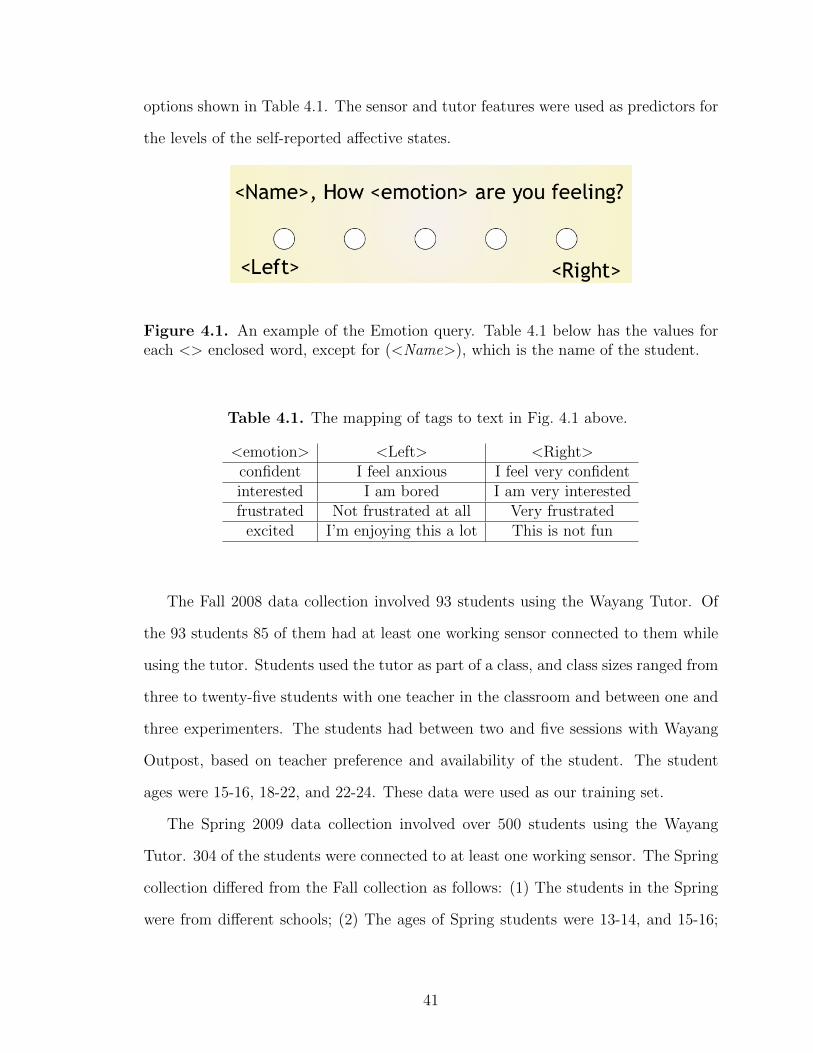
options shown in Table 4.1. The sensor and tutor features were used as predictors for
the levels of the self-reported affective states.
Figure 4.1. An example of the Emotion query. Table 4.1 below has the values foreach <> enclosed word, except for (<Name>), which is the name of the student.
Table 4.1. The mapping of tags to text in Fig. 4.1 above.
<emotion> <Left> <Right>confident I feel anxious I feel very confidentinterested I am bored I am very interestedfrustrated Not frustrated at all Very frustrated
excited I’m enjoying this a lot This is not fun
The Fall 2008 data collection involved 93 students using the Wayang Tutor. Of
the 93 students 85 of them had at least one working sensor connected to them while
using the tutor. Students used the tutor as part of a class, and class sizes ranged from
three to twenty-five students with one teacher in the classroom and between one and
three experimenters. The students had between two and five sessions with Wayang
Outpost, based on teacher preference and availability of the student. The student
ages were 15-16, 18-22, and 22-24. These data were used as our training set.
The Spring 2009 data collection involved over 500 students using the Wayang
Tutor. 304 of the students were connected to at least one working sensor. The Spring
collection differed from the Fall collection as follows: (1) The students in the Spring
were from different schools; (2) The ages of Spring students were 13-14, and 15-16;
41
(3) The camera sensor in the Spring had upgraded software. The Spring Data was
used purely for validation of the Fall Data.
4.3.2 Tutor and Sensor Features
We considered nine tutor features and forty sensor features as potential predictors
for the emotion classifiers (see Table 4.2). The forty sensor features are based on
four ways of summarizing ten specific features: the mean, the standard deviation,
the min value, and the max value over the course of a problem. Since the sensor
and tutor logging happens asynchronously, their data are interpolated in a piecewise
constant fashion with the constraint that only data from the past is used to predict
missing sensor or tutor values. The tutor logs when a problem is opened and closed,
creating boundaries for summarizing the interpolated sensor data (i.e. to compute
each feature, we use data over the span of a single problem). When there is an
emotional query after a problem, the result becomes the affective state label for that
problem. For each student and for each emotion there are between two and five
affective-state labels. For more detail on the full specification of these features see
Chapter 3.
4.4 Method
The current standards for evaluating affective classifiers do not address our need to
rank classifiers for the purpose of actionable affect detection. Though each individual
step in our method has been established and tested, the combination of these steps
yields a more robust test for the classifiers constructed. The use of our classifiers in a
classroom environment necessitates our method described in the rest of this section
and summarized in Table 4.3.
42

Table 4.2. Features used for each problem that includes an affective state label inorder to train the emotion classifiers (features are shown in abbreviated form). Thenine tutor features are shown on the left and the ten sensor features are on the right.Features used in a classifier that are significantly better than the baseline (p < 0.05)are in bold.
Tutor feature Definition Sensor feature DefinitionSolv. on 1st 1st attempt cor-
rectAgreeing
camera mental statesSec. to 1st time to 1st at-tempt
Concentrating
Sec. to solv. time to a correct Thinking# incorrect responses Interested# hints requested UnsureLC learning
companionMouse sum of pressure
Groupwhich LC Sit Forward
movement in chair(Jake, Jane, ornone)
Seat change
Time insession
same day Back change
Time in tutor all days Skinconductance
value from wrist
43

4.4.1 Collection
The data collection described in Sec. 4.3 is the first step in our methodology for
building affect classifiers. The key parts of the data collection are that the emotion
labels are made at the time of the experience, and the training and validation sets are
taken from distinct populations using the same basic setup, allowing the validation
results to be more likely to generalize. Here, the Fall collection is our training data
set and the Spring collection is our validation data set.
4.4.2 Predictor Selection
Once the data were collected and summarized as described in Sec. 4.3.2, we used
the entire set of labeled training data to create a subset of predictors using a combi-
nation of tutor and sensor features. For each combination of features, a subset of the
data set that was not missing data for the features was selected. Then stepwise linear
regression was performed in R, an open source statistical package [98], to select the
‘best’ subset of features from those available. The subset of features was stored as a
formula for use in training the classifiers and performing cross-validation.
4.4.3 Cross-Validation
For each set of features determined by the feature selection, we performed leave-
one-student-out cross-validation on linear classifiers for each affective state. During
the cross-validation, we calculated the mean accuracy, sensitivity, and specificity for
each test student. We also performed the same cross-validation on a linear classifier
with a constant model, which we used as our baseline. This step differs from [31] in
two ways: 1) The mean was taken across each test student instead of across tests. 2)
We calculated sensitivity and specificity in addition to accuracy.
Though the cross-validation described above provides a general indication of the
performance of each classifier, the information is not sufficient to enable appropriate
pedagogical action selection by an ITS for new populations of students. Thus, we
44
validated that the classifiers are generalizable and so can be used with a new pop-
ulation without having to be retrained. We also ranked the classifiers according to
how sensors and features impact accuracy, allowing us to make informed decisions
about sensor selection (e.g., if some sensors become unavailable, to select the next
best alternative).
4.4.4 Classifier Ranking
A number of alternative techniques exist for classifier comparison. One is to use
classifier accuracy, which identifies the overall performance of a classifier, but does
not express accuracy on positive vs. negative instances. To do so, the following
two measures can be used: (1) sensitivity, also referred to as the true positive rate,
which provides information about the accuracy of a positive response; (2) specificity,
the true negative rate, which provides information about the accuracy of negative
responses.
Since the purpose of our classifiers is to help an ITS make decisions of how to
appropriately respond to student emotion, one approach would be to only make a
decision when there is confidence in the prediction. So, if one classifier has very good
sensitivity relative to the baseline, then the ITS would act when the classifier reports
a positive result. Similarly, if a classifier has a very good specificity relative to the
baseline, then the ITS would act when the classifier reports a negative result.
In order to compare our classifiers’ accuracy, sensitivity, and specificity for each
affective state, we first performed a one-way analysis of variance (ANOVA), with each
classifier as the independent variable and either accuracy, sensitivity, or specificity as
the dependent variable. When there was a significant difference between classifiers,
we performed Tukey’s HSD test to rank the differences in the means. Tukey’s HSD
test is a parametric multiple comparison test to find which means are significantly
different from each other [126].
45
There is some question about the soundness of the ANOVA and Tukey’s HSD test
for these comparisons because the design is not balanced (not every student had all
sensors available), and the responses are not normally distributed. So, in addition to
the ANOVA, a Kruskal-Wallace test was performed; when there was a significant dif-
ference between classifiers, a nonparametric multiple comparison procedure (NPMC)
for an unbalanced one-way layout was performed, as described in [86].
We conducted both parametric and non-parametric tests because the parametric
tests are known to be robust to violations of the assumptions, so performing both was
a way to verify the findings. Here, for all tests, we only report results with significant
differences.
4.4.5 Validation with Follow-on Data
As mentioned above, we used the Spring 2009 data set to validate the classifiers
trained on the Fall 2008 data set (the Spring data set was not used to inform any of
the training). The validation consisted of the following three steps. First, for each
feature set selected by the feature selection step, a linear classifier was created using
the entire subset described in Sec. 4.4.2. Second, each classifier was tested on the
relevant subset of data from the Spring data set. Third, the accuracy, sensitivity,
and specificity values and rankings were compared to the cross-validated values and
rankings to determine how the classifiers generalized to a new and larger population.
4.5 Results
The classifier sets were designed to compare the performance of (1) a classifier
using just tutor features vs. (2) one using features from one sensor in addition to the
tutor features vs. (3) a classifier using all of the available features. The collection,
feature selection, and cross-validation results from the training data (Fall 2008) are
described in Chapter 3 [31]; however, a couple of important details are needed here.
46
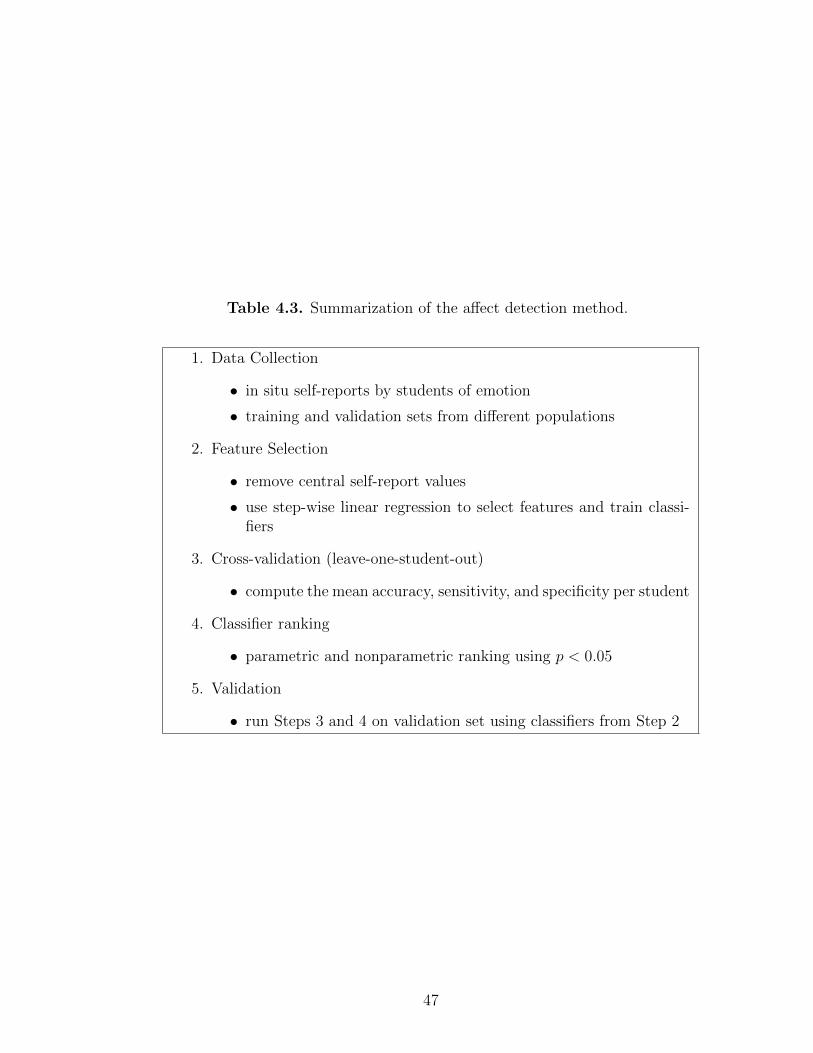
Table 4.3. Summarization of the affect detection method.
1. Data Collection
• in situ self-reports by students of emotion
• training and validation sets from different populations
2. Feature Selection
• remove central self-report values
• use step-wise linear regression to select features and train classi-fiers
3. Cross-validation (leave-one-student-out)
• compute the mean accuracy, sensitivity, and specificity per student
4. Classifier ranking
• parametric and nonparametric ranking using p < 0.05
5. Validation
• run Steps 3 and 4 on validation set using classifiers from Step 2
47
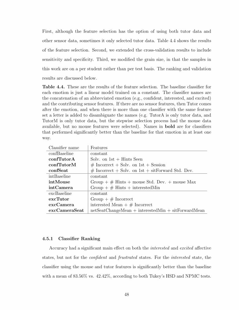
First, although the feature selection has the option of using both tutor data and
other sensor data, sometimes it only selected tutor data. Table 4.4 shows the results
of the feature selection. Second, we extended the cross-validation results to include
sensitivity and specificity. Third, we modified the grain size, in that the samples in
this work are on a per student rather than per test basis. The ranking and validation
results are discussed below.
Table 4.4. These are the results of the feature selection. The baseline classifier foreach emotion is just a linear model trained on a constant. The classifier names arethe concatenation of an abbreviated emotion (e.g., confident, interested, and excited)and the contributing sensor features. If there are no sensor features, then Tutor comesafter the emotion, and when there is more than one classifier with the same featureset a letter is added to disambiguate the names (e.g. TutorA is only tutor data, andTutorM is only tutor data, but the stepwise selection process had the mouse dataavailable, but no mouse features were selected). Names in bold are for classifiersthat performed significantly better than the baseline for that emotion in at least oneway.
Classifier name FeaturesconfBaseline constantconfTutorA Solv. on 1st + Hints SeenconfTutorM # Incorrect + Solv. on 1st + SessionconfSeat # Incorrect + Solv. on 1st + sitForward Std. Dev.intBaseline constantintMouse Group + # Hints + mouse Std. Dev. + mouse MaxintCamera Group + # Hints + interestedMinexcBaseline constantexcTutor Group + # IncorrectexcCamera interested Mean + # IncorrectexcCameraSeat netSeatChangeMean + interestedMin + sitForwardMean
4.5.1 Classifier Ranking
Accuracy had a significant main effect on both the interested and excited affective
states, but not for the confident and frustrated states. For the interested state, the
classifier using the mouse and tutor features is significantly better than the baseline
with a mean of 83.56% vs. 42.42%, according to both Tukey’s HSD and NPMC tests.
48
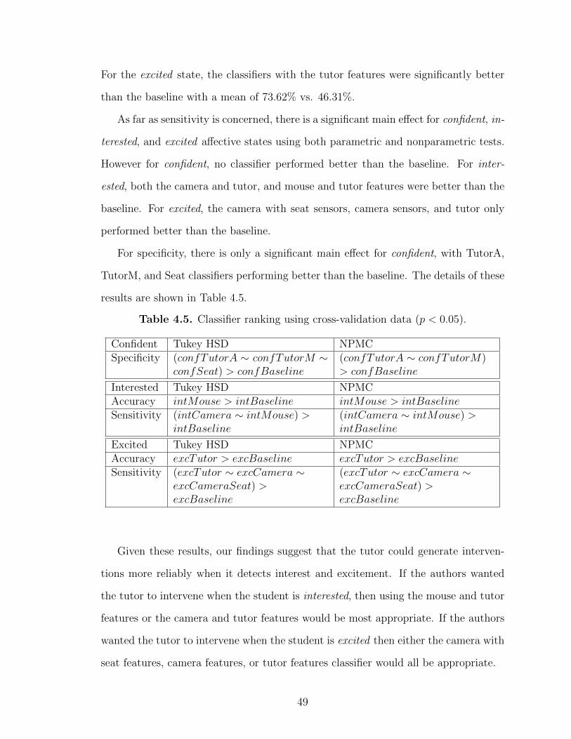
For the excited state, the classifiers with the tutor features were significantly better
than the baseline with a mean of 73.62% vs. 46.31%.
As far as sensitivity is concerned, there is a significant main effect for confident, in-
terested, and excited affective states using both parametric and nonparametric tests.
However for confident, no classifier performed better than the baseline. For inter-
ested, both the camera and tutor, and mouse and tutor features were better than the
baseline. For excited, the camera with seat sensors, camera sensors, and tutor only
performed better than the baseline.
For specificity, there is only a significant main effect for confident, with TutorA,
TutorM, and Seat classifiers performing better than the baseline. The details of these
results are shown in Table 4.5.
Table 4.5. Classifier ranking using cross-validation data (p < 0.05).
Confident Tukey HSD NPMCSpecificity (confTutorA ∼ confTutorM ∼
confSeat) > confBaseline(confTutorA ∼ confTutorM)> confBaseline
Interested Tukey HSD NPMCAccuracy intMouse > intBaseline intMouse > intBaselineSensitivity (intCamera ∼ intMouse) >
intBaseline(intCamera ∼ intMouse) >intBaseline
Excited Tukey HSD NPMCAccuracy excTutor > excBaseline excTutor > excBaselineSensitivity (excTutor ∼ excCamera ∼
excCameraSeat) >excBaseline
(excTutor ∼ excCamera ∼excCameraSeat) >excBaseline
Given these results, our findings suggest that the tutor could generate interven-
tions more reliably when it detects interest and excitement. If the authors wanted
the tutor to intervene when the student is interested, then using the mouse and tutor
features or the camera and tutor features would be most appropriate. If the authors
wanted the tutor to intervene when the student is excited then either the camera with
seat features, camera features, or tutor features classifier would all be appropriate.
49
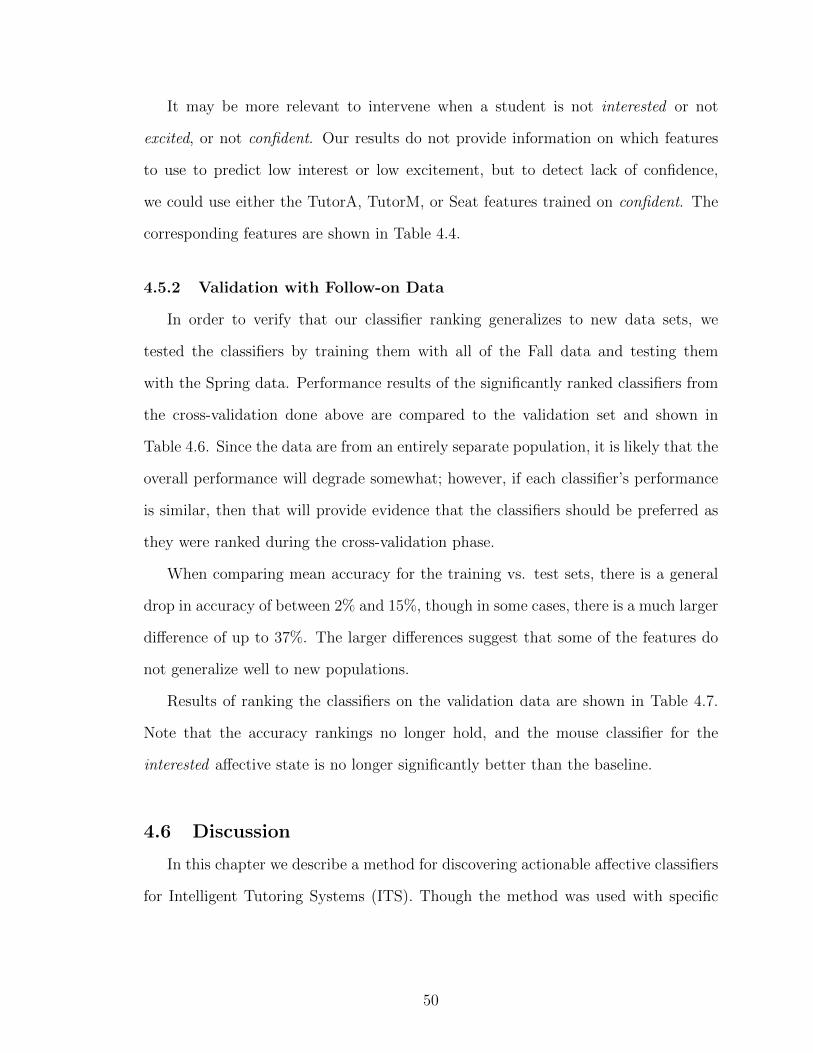
It may be more relevant to intervene when a student is not interested or not
excited, or not confident. Our results do not provide information on which features
to use to predict low interest or low excitement, but to detect lack of confidence,
we could use either the TutorA, TutorM, or Seat features trained on confident. The
corresponding features are shown in Table 4.4.
4.5.2 Validation with Follow-on Data
In order to verify that our classifier ranking generalizes to new data sets, we
tested the classifiers by training them with all of the Fall data and testing them
with the Spring data. Performance results of the significantly ranked classifiers from
the cross-validation done above are compared to the validation set and shown in
Table 4.6. Since the data are from an entirely separate population, it is likely that the
overall performance will degrade somewhat; however, if each classifier’s performance
is similar, then that will provide evidence that the classifiers should be preferred as
they were ranked during the cross-validation phase.
When comparing mean accuracy for the training vs. test sets, there is a general
drop in accuracy of between 2% and 15%, though in some cases, there is a much larger
difference of up to 37%. The larger differences suggest that some of the features do
not generalize well to new populations.
Results of ranking the classifiers on the validation data are shown in Table 4.7.
Note that the accuracy rankings no longer hold, and the mouse classifier for the
interested affective state is no longer significantly better than the baseline.
4.6 Discussion
In this chapter we describe a method for discovering actionable affective classifiers
for Intelligent Tutoring Systems (ITS). Though the method was used with specific
50
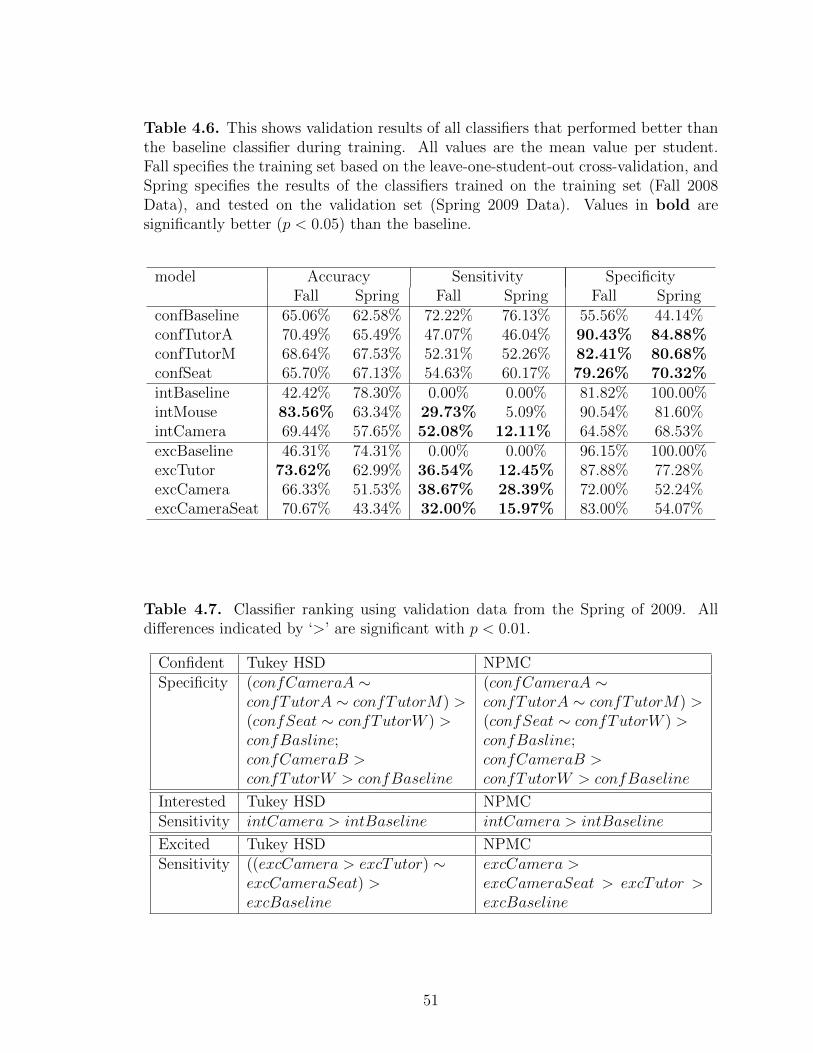
Table 4.6. This shows validation results of all classifiers that performed better thanthe baseline classifier during training. All values are the mean value per student.Fall specifies the training set based on the leave-one-student-out cross-validation, andSpring specifies the results of the classifiers trained on the training set (Fall 2008Data), and tested on the validation set (Spring 2009 Data). Values in bold aresignificantly better (p < 0.05) than the baseline.
model Accuracy Sensitivity SpecificityFall Spring Fall Spring Fall Spring
confBaseline 65.06% 62.58% 72.22% 76.13% 55.56% 44.14%confTutorA 70.49% 65.49% 47.07% 46.04% 90.43% 84.88%confTutorM 68.64% 67.53% 52.31% 52.26% 82.41% 80.68%confSeat 65.70% 67.13% 54.63% 60.17% 79.26% 70.32%intBaseline 42.42% 78.30% 0.00% 0.00% 81.82% 100.00%intMouse 83.56% 63.34% 29.73% 5.09% 90.54% 81.60%intCamera 69.44% 57.65% 52.08% 12.11% 64.58% 68.53%excBaseline 46.31% 74.31% 0.00% 0.00% 96.15% 100.00%excTutor 73.62% 62.99% 36.54% 12.45% 87.88% 77.28%excCamera 66.33% 51.53% 38.67% 28.39% 72.00% 52.24%excCameraSeat 70.67% 43.34% 32.00% 15.97% 83.00% 54.07%
Table 4.7. Classifier ranking using validation data from the Spring of 2009. Alldifferences indicated by ‘>’ are significant with p < 0.01.
Confident Tukey HSD NPMCSpecificity (confCameraA ∼
confTutorA ∼ confTutorM) >(confSeat ∼ confTutorW ) >confBasline;confCameraB >confTutorW > confBaseline
(confCameraA ∼confTutorA ∼ confTutorM) >(confSeat ∼ confTutorW ) >confBasline;confCameraB >confTutorW > confBaseline
Interested Tukey HSD NPMCSensitivity intCamera > intBaseline intCamera > intBaseline
Excited Tukey HSD NPMCSensitivity ((excCamera > excTutor) ∼
excCameraSeat) >excBaseline
excCamera >excCameraSeat > excTutor >excBaseline
51
sensors, features, ITS and classifiers based on linear models, each of these could
conceivably be swapped out for another system.
Our results identify a clear ranking for three classifiers designed to detect low
student confidence, one classifier to detect interest, and three classifiers to detect
excitement. For not confident, two different sets of tutor only features performed
better than the tutor and seat features, so it is unlikely that there would be a time
that we would use the classifier with the seat sensor.
Now that we have actionable classifiers for three affective states, our ITS will be
able to leverage the results to make a decision. For instance, the ITS could intervene
whenever the classifier detects low student confidence, in order to help the student
gain self efficacy. This intervention will have to also take into account other emotions
detected, e.g., the detection of high excitement and/or high interest may change the
type of intervention that is most appropriate.
Future work will involve implementing these various affect-based interventions,
and evaluating their impact on student learning, affect and motivation. We also plan
to explore how we can design classifiers for affect recognition that perform better than
the baseline for the subset of affective states on which our classifiers performed poorly.
One approach for doing so that we plan to implement is to identify more complex
features based on the sensor data than those currently used. A more complete set of
affective classifiers will likely improve the ITS interventions. For example, if we had
a classifier that had good sensitivity for confidence, then that classifier could be used
to stop interventions relating to low confidence.
52

CHAPTER 5
SPEAKER DIFFERENCES AND HEALTH DIAGNOSIS
The intersection of emotion and health is most clear in voice production, and
the field of communication disorders utilizes the voice for diagnosis of a variety of
problems. One of the oldest recorded voice related communication disability was
that of Mursilis, a Hittite king from 1344-1320 B.C.E. [41]. In a cuneiform text,
Mursilis describes his fear causing his loss of speech a number of times during his life.
With the creation of the telephone, tools became available to study voice [34],
and since the early twentieth century empirical studies of specific vocal features such
as pitch and intensity have been studied in relation to emotion, such as differentia-
tion between feeling happy and sad [118], and health, such as what is typical [88],
characteristics of Parkinson’s [24], and characteristics of a cleft palate [63].
5.1 Related Work
McCauley and Strand performed a review of standardized tests to diagnose child-
hood apraxia of speech (CAS) and found that the tests do not adequately address
“relevant psychometric principles” [79]. The two metrics that are commonly used to
aid in the diagnosis of CAS are the lexical speech ratio (LSR) [113], and the coeffi-
cient of variation ratio (CVR) [114]. There is a proposed computational method for
diagnosis of CAS with these two features [64], however this method still requires the
manual time alignment of phonemes from each subject. Since this is a labor intensive
process, fully automated computational methods are desirable.
53
The diagnosis of Austistic Spectrum Disorders (ASD) involves many methods
including evaluating voice production [52]. McCann and Peppe reviewed studies in-
volved with the symptom of unusual prosody in Autism Spectrum Disorder (ASD) to
determine if a standard quantitative measure has been established, and they found a
lot of disagreement in the literature [78]. Since then, Velleman, Andrianopoulos, et
al., studied differences in children with neurodevelopmental problems such as CAS
and ASD, and noted significant differences in motor speech and voice between these
two groups and their typically developing peers [127]. In addition, Paul et al., con-
ducted a study on both the perception and production of prosodic features [94]. The
authors found that there were significantly more errors for ASD subjects than typi-
cally developing (TD) subjects when it came to producing the correct lexical stress.
Specifically when given the instructions to pronounce the word recall as “re call” as
opposed to “re call” when reading the sentence “I can’t recall his name.”
There have been a number of computational approaches to distinguish pathological
voices from healthy voices. One example is Fonseca et al., who use linear prediction
coefficients (LPC) and a discrete wavelet transform (DWT-db) with a least square
support vector machine to determine whether a patient has a pathology, nodules or
vocal folds, or whether the patient is healthy [54]. In addition, some work has been
done to automatically detect negative symptoms in schizophrenia [29]. The authors
used the standard deviation of F0 during a 50 ms frame as the inflection. Alogia, or
poverty of speech, was computed as words per minute, or total word count divided by
total time of patient speaking. Additionally computerized lexical analysis was done
after the data was transcribed by human laboratory assistants.
We use non-lexical acoustic features that have been used in the past as well as
novel features for the computational classification of gender and different cultures.
54

5.2 Experimental Setup : Multicultural Study
In the current multicultural study, ten participants were studied, comprised of 5
males and 5 females per culture/race. Mandarin Chinese, Hindi Indian, Caucasian
American, and African American males and females were matched within 15% by age,
height, and weight. Acoustic measures of each participant were collected in a sound
proof room to minimize contamination of the acoustic signal due to ambient noise
levels. Participants’ voices were recorded using a TASCAM DA-P1 DAT recorder and
a condenser microphone positioned one inch and 45◦ off axis from the participant’s
mouth. More detailed information about the highly controlled conditions can be
found in work from 2001 of Andrianopoulos et al., [5, 6]. Participants performed a
number of speech tasks. Tasks included vowel production and spontaneous speech.
The vowels, [a] (as in the word ‘ah’), [i] (as in the word ‘eat’) and [u] (as in the word
‘glue’), were selected for the study because they are universal across cultures. Three
tokens of 600 ms were obtained for each vowel. The spontaneous speech samples were
obtained in order to analyze connected speech characteristics. The order of the tasks
was as follows:
1. Pronounce three prolonged vowels:
[a] (as in the word ‘ah’)
[i] (as in the word ‘eat’)
[u] (as in the word ‘glue’)
2. speak demographic information in English
3. speak demographic information in native language
4. describe picture 1 in English
5. describe picture 2 in English
55
6. describe picture 1 in native language
7. describe picture 2 in native language
5.3 Classification
There are a number of ways to categorize speakers from the multicultural data.
It is less challenging to identify speakers by gender. It is desirable to identify those
features that distinguish between each culture and race; however, this is a four class
classification problem, and it’s much less likely that simple linear least squares re-
gression will do well for this number of classes. Another way to split the data is by
native English speakers vs. non-native English speakers.
The multi-class version of the simple linear least squares classifier actually requires
that four separate classifiers are trained, and the class is selected by which classifier
gives the highest score. There are some potential problems with this approach when
applying it to simple linear least squares models; however, the basic method for
multi-class classification is the same.
The acoustic features that we use for classification are derived from pitch, intensity,
and time and are shown in Table 5.1.
Features are collected by first segmenting the speech files of each subject into
utterances. The utterances are defined by different length pauses, where a pause is
defined by the intensity of the recording going and staying below 60 dB for a specific
length of time. The pause length minimums that we check are 100 ms, 150 ms, 200
ms, 500 ms, 800 ms, 900 ms, 1000 ms, 1100 ms, and 1200 ms. For each pause length
we either add a 100 ms buffer on either side of the utterance (if there is space to do
so) or we add no buffer to the utterance. The addition of the buffer increases the size
of the utterance, but does not modify the sound in any way.
Once we have each of the utterances, prolonged vowels and unspoken sounds were
automatically removed from the set of utterances using a heuristic as follows. If
56

Table 5.1. The ten acoustical features below are selected by using a linear leastsquares stepwise regression models to predict gender, American vs. Asian culture,or one of four cultures. This table lists each feature with an abbreviation and adefinition.
Feature Abbreviation DefinitionPitch Mean Hz meanF0 The mean F0 of the utterance in Hz.Pitch Stdev Hz stdevF0 The stdev F0 of the utterance.Pitch Min Hz minF0 The min F0 of the utterance.Pitch Max Hz maxF0 The max F0 of the utterance.Pitch Change changeF0 The mean absolute slope of F0 in
Hz of the utterance.Intensity Mean dB meanI The mean I of the utterance.Intensity Stdev dB stdevI The stdev I of the utterance.Intensity Min dB minI The min I of the utterance.Intensity Max dB maxI The max I of the utterance.
Ratio Voiced %voiced The ratio of voiced to total numberof frames in the utterance.
the %voiced feature is between 20% and 80%, then it is considered natural speech.
Otherwise it is discarded. This was done because the natural speech data is more
relevant for other studies that record natural speech rather than scripted speech that
is ideal for data collection. We use the same method of stepwise linear least squares
regression and leave one subject out cross-validation on a linear least squares classifier
as we do for the Computer Based Education work described in Chapter 3.
5.4 Results
The gender classifiers performed best when the utterances were defined as being
separated by pauses of at least 150-200 ms with no buffer. Figure 5.1 shows the
relationship of minimum pause time differentiating utterances and the classification
accuracy. Accuracies range from 84% to 93%. The features selected for gender that
serve as the best classifiers were: meanF0 , stdevF0 ,maxF0 ,minF0 ,meanI ,maxI ,stdevI ,
and changeF0 as defined in Table 5.1.
57
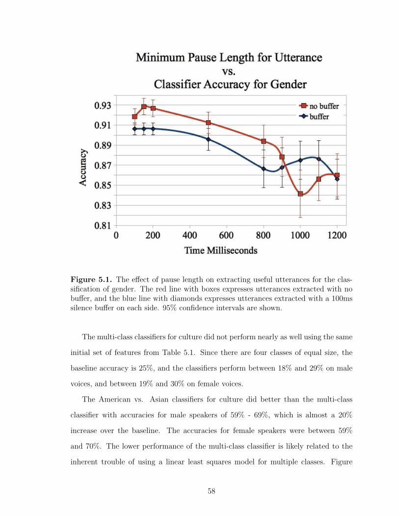
Figure 5.1. The effect of pause length on extracting useful utterances for the clas-sification of gender. The red line with boxes expresses utterances extracted with nobuffer, and the blue line with diamonds expresses utterances extracted with a 100mssilence buffer on each side. 95% confidence intervals are shown.
The multi-class classifiers for culture did not perform nearly as well using the same
initial set of features from Table 5.1. Since there are four classes of equal size, the
baseline accuracy is 25%, and the classifiers perform between 18% and 29% on male
voices, and between 19% and 30% on female voices.
The American vs. Asian classifiers for culture did better than the multi-class
classifier with accuracies for male speakers of 59% - 69%, which is almost a 20%
increase over the baseline. The accuracies for female speakers were between 59%
and 70%. The lower performance of the multi-class classifier is likely related to the
inherent trouble of using a linear least squares model for multiple classes. Figure
58
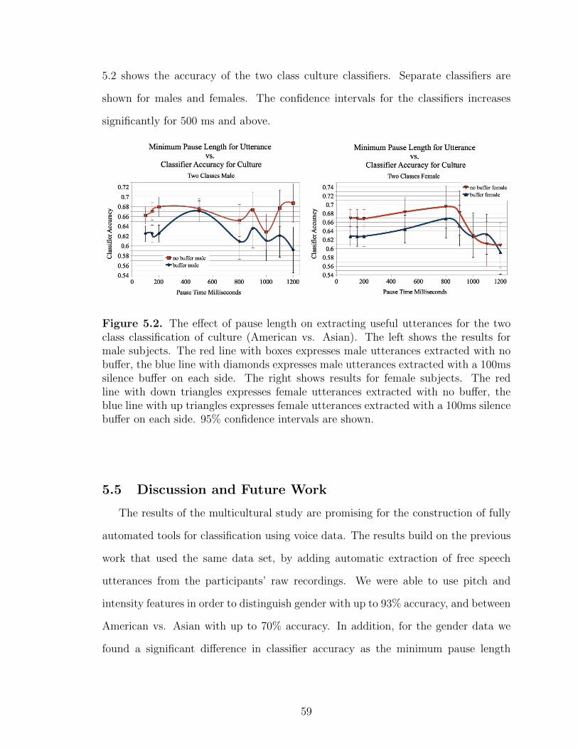
5.2 shows the accuracy of the two class culture classifiers. Separate classifiers are
shown for males and females. The confidence intervals for the classifiers increases
significantly for 500 ms and above.
Figure 5.2. The effect of pause length on extracting useful utterances for the twoclass classification of culture (American vs. Asian). The left shows the results formale subjects. The red line with boxes expresses male utterances extracted with nobuffer, the blue line with diamonds expresses male utterances extracted with a 100mssilence buffer on each side. The right shows results for female subjects. The redline with down triangles expresses female utterances extracted with no buffer, theblue line with up triangles expresses female utterances extracted with a 100ms silencebuffer on each side. 95% confidence intervals are shown.
5.5 Discussion and Future Work
The results of the multicultural study are promising for the construction of fully
automated tools for classification using voice data. The results build on the previous
work that used the same data set, by adding automatic extraction of free speech
utterances from the participants’ raw recordings. We were able to use pitch and
intensity features in order to distinguish gender with up to 93% accuracy, and between
American vs. Asian with up to 70% accuracy. In addition, for the gender data we
found a significant difference in classifier accuracy as the minimum pause length
59
changes between 200 ms and 500 ms. This suggests that the optimal pause length to
automatically segment speech is between 100 and 200 ms.
A linear least squares classification for the multi-class culture categorization was
insufficient. This is likely due to two explanations: 1) linear least squares classification
is known to have difficulty with more than two categories; 2) the number of subjects
in each class is two small to find the differences that would be readily apparent. A
third explanation would be that the features available are not useful for categorization
of cultural differences. However, if this were the case then the two class version of
the culture classifier wouldn’t have performed well.
The fact that the features selected for both culture and gender were very similar
is problematic for the goal of finding independent features for each type of categoriza-
tion. The one feature that was selected for gender, but was not selected for culture
differentiation is %voiced. This feature is a good place to start. In addition, we only
looked at the statistics of individual utterances, and we did not look at the sequence
of utterances and how they change over time. A future step is to study how utter-
ances change over time. However, we anticipate difficulties with this approach as
the sequence lengths get longer, since there will be fewer samples per participant.
In addition, increasing the number and type of variables for study may increase the
accuracy and validity for these analyses. For example, this research only studied
pitch (fundamental frequency) and other analyses of measurements on pitch signals
and intensity. It is prudent to study other features of the acoustic signal, such as
differences in short- and long-term frequency and amplitude perturbation, especially
for health diagnosis, noise to harmonics ratio, percent tremor, soft phonation index,
and number of semitones, to name some. Many of these named features are typically
evaluated on prolonged vowel data or on phrases that are identical, so new methods
are needed in order to apply them to the free speech samples in question in this
research.
60

CHAPTER 6
HEALTH CARE EDUCATION
Health Care education includes a practical component that does not easily trans-
late to a typical computer tutoring system. For example, in a practical scenario for
a nurse in training, the student must be able to physically interact with the patient
in order to learn the appropriate response to a patient’s needs. Clinical simulation
environments are often used in order to reduce the number of people required to train
a nurse while allowing them to receive practical experience before interacting with
real patients [109, 95, 59]. These simulation environments are used for the evaluation
of the student nurses. During the evaluations, student nurses are video and audio
recorded. This video and audio recording is a place where computational assistance
can be given to the instructors. In this chapter we present computational detection
of emotion in a clinical simulation to help an instructor determine if a student is at
a higher risk of leaving the program. We discuss clinical simulation, video detection
of emotion, audio detection of emotion. Then we describe an experiment involving
student nurses self-reporting their emotion before and after their clinical evaluation.
Finally, we show the results of detecting affect in the above mentioned experiment.
6.1 Clinical Simulation
Since the 1960’s, mannequins have been used for medical training [32]. The first
success is Resusci R©-Anne, which was made so that people could learn mouth to
mouth ventilation. Many different mannequin systems have been created with a vari-
ety of acceptance. Recently, the clinical simulation has been added to the curriculum
61
of student nurses [95, 59]. One skill that is practiced with these simulators is a ten
minute patient assessment [133], in which the student nurse is evaluated while in-
teracting with a simulated patient. The student nurse is in a room alone with the
simulated patient. The instructor remotely provides the voice of the patient in the
room and the doctor on the other end of the phone. There are realisitic props that
are typical in a hospital room, including a monitor, a method for providing air to
the patient, and a way to provide intravenous (IV) fluids to the patient. In addition,
the mannequin produces sounds like a heartbeat and breathing when observed with a
stethoscope. The limbs can also show ailments on them. The clinical simulation labs
are fitted with a camera and microphone so that students in a classroom can watch
the simulation, and/or the simulation can be recorded on DVD for future viewing.
As students become more familiar with the simulator, they watch a video of their
own evaluation as part of the evaluation process, after which they discuss their per-
formance with the instructor.
6.2 Experimental Setup
52 subjects were recruited for the study, 3 students left the study leaving 4 male
and 45 female subjects. Subjects were all in a four-year undergraduate bachelor of
science program for preparation to become registered nurses. Subjects were either in
their third or fourth year of the program. This study involves giving two surveys,
one before and one after the simulation test. In addition, the DVD recording of the
simulation test that is already used as part of the student’s test, was collected and
archived for computational analysis. The order of the protocol is as follows: Subjects
were briefed on the study. A pre-test survey of emotion was given to the subjects.
Subjects took their simulation test while being recorded in video and audio on a DVD.
A post-test survey of emotion was given to the subjects. Subjects performed a self-
assessment by viewing the DVD of their test. Subjects discussed their performance
62
with their teacher. DVDs and surveys were collected at the end, and students were
debriefed in case they had any questions or concerns. Of the 49 subjects one subject
withdrew from the experiment, and one subject did not complete the post-test survey.
6.3 Video Features
The goal of this study was to determine whether the location and activity of the
student nurses, as extracted by state of the art computer vision algorithms, are useful
for the detection of emotions related to learning environments. The emotions that
are in question were confidence, anxiety, interest, excitement, and frustration.
Due to the setting of the study, video recordings are different from most studies
involving using video to detect emotion, and it was also different from most studies
involving tracking a person. The first major difference in this study was that the face
of the subject was rarely, if ever, in view of the camera. This precluded the use of
facial expression analysis for the purpose of emotion. The second major difference
was that there are no markers or other ground truth information for tracking. In
some studies, when there are no markers used, and no ground truth information for
position, the person being tracked wore clothing of a color in high contrast to the
background, and the room had a background color that was different from the skin
tone and clothing of the subjects.
Given that the subjects were being evaluated by their instructors, the environment
could not be changed to make it easier on the vision algorithms. This meant that the
students were wearing white shirts in a room painted off-white, and with off-white
linens.
The lack of ground truth information for the tracks meant that the tracking algo-
rithms were evaluated qualitatively, and a number of competing tracking algorithms
were used to get the distances to key points at each frame.
63
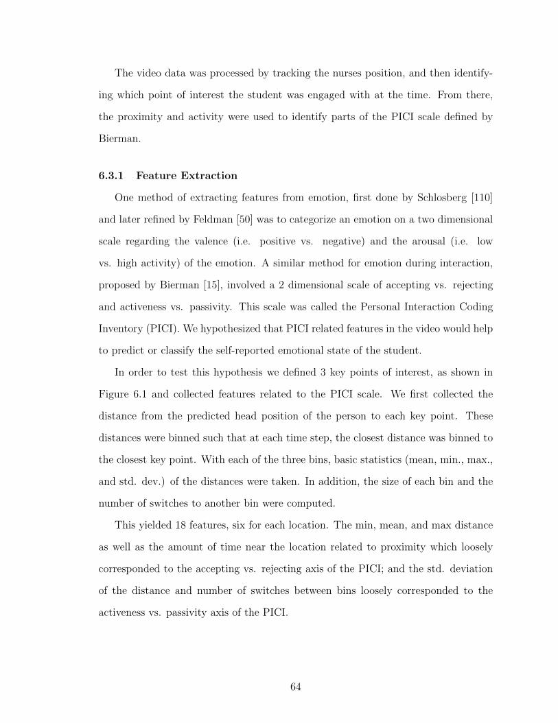
The video data was processed by tracking the nurses position, and then identify-
ing which point of interest the student was engaged with at the time. From there,
the proximity and activity were used to identify parts of the PICI scale defined by
Bierman.
6.3.1 Feature Extraction
One method of extracting features from emotion, first done by Schlosberg [110]
and later refined by Feldman [50] was to categorize an emotion on a two dimensional
scale regarding the valence (i.e. positive vs. negative) and the arousal (i.e. low
vs. high activity) of the emotion. A similar method for emotion during interaction,
proposed by Bierman [15], involved a 2 dimensional scale of accepting vs. rejecting
and activeness vs. passivity. This scale was called the Personal Interaction Coding
Inventory (PICI). We hypothesized that PICI related features in the video would help
to predict or classify the self-reported emotional state of the student.
In order to test this hypothesis we defined 3 key points of interest, as shown in
Figure 6.1 and collected features related to the PICI scale. We first collected the
distance from the predicted head position of the person to each key point. These
distances were binned such that at each time step, the closest distance was binned to
the closest key point. With each of the three bins, basic statistics (mean, min., max.,
and std. dev.) of the distances were taken. In addition, the size of each bin and the
number of switches to another bin were computed.
This yielded 18 features, six for each location. The min, mean, and max distance
as well as the amount of time near the location related to proximity which loosely
corresponded to the accepting vs. rejecting axis of the PICI; and the std. deviation
of the distance and number of switches between bins loosely corresponded to the
activeness vs. passivity axis of the PICI.
64
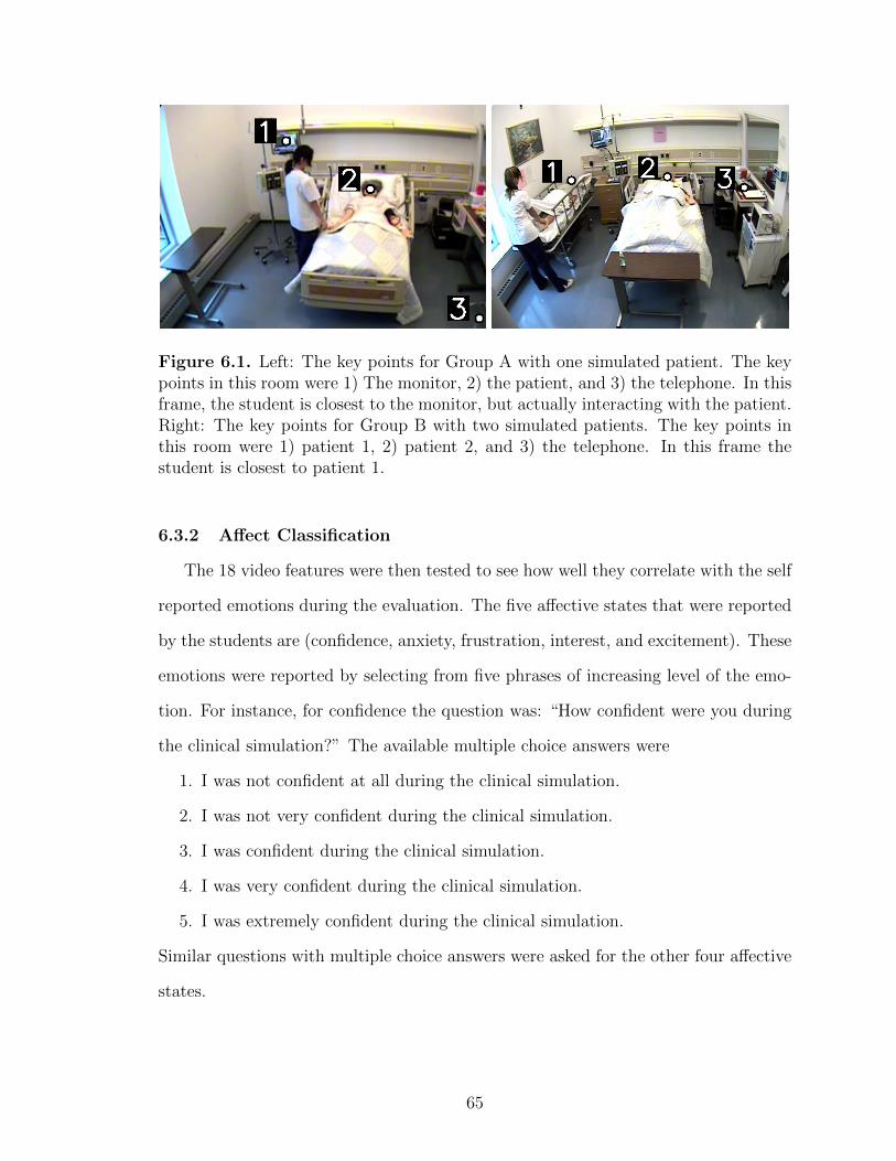
Figure 6.1. Left: The key points for Group A with one simulated patient. The keypoints in this room were 1) The monitor, 2) the patient, and 3) the telephone. In thisframe, the student is closest to the monitor, but actually interacting with the patient.Right: The key points for Group B with two simulated patients. The key points inthis room were 1) patient 1, 2) patient 2, and 3) the telephone. In this frame thestudent is closest to patient 1.
6.3.2 Affect Classification
The 18 video features were then tested to see how well they correlate with the self
reported emotions during the evaluation. The five affective states that were reported
by the students are (confidence, anxiety, frustration, interest, and excitement). These
emotions were reported by selecting from five phrases of increasing level of the emo-
tion. For instance, for confidence the question was: “How confident were you during
the clinical simulation?” The available multiple choice answers were
1. I was not confident at all during the clinical simulation.
2. I was not very confident during the clinical simulation.
3. I was confident during the clinical simulation.
4. I was very confident during the clinical simulation.
5. I was extremely confident during the clinical simulation.
Similar questions with multiple choice answers were asked for the other four affective
states.
65
The self-reports were collected immediately following the clinical part of the evalu-
ation, and before the student nurse watched the video of themselves. This was so that
the recollection of their emotion would be freshest in their mind without interrupting
the evaluation process.
6.3.3 Pre-processing
The first step of processing the video is to track the position of the student. Before
the above experiment was performed, some preliminary video recordings were taken
using a similar setup. These videos were used to determine which tracking algorithm
would be used for the study.
6.3.3.1 Person Tracking
The problem of tracking people has been researched in many contexts. Tracking a
student nurse in a clinical simulation room is similar to other applications of tracking
one person in a room, but there are some key differences. First, the person is much
more likely to be facing away from the camera rather than towards it. This is because
the camera was positioned to face the simulated patients not the students. Second,
the person was typically wearing a white shirt and dark (usually black) pants. Third,
much of the room was white or off white in color. In addition, video segments for
tracking a person are between ten and thirty minutes in length, and occasionally the
person leaves the field of view of the camera.
A number of available implementations of person tracking and detection systems
were considered. These include the Reading People Tracker, a pose tracker, the
CAMSHIFT tracker, upper body detectors, a Lucas-Kanade feature tracker, and hog
based person detection.
Initially, the Reading People Tracker [116] appeared to be a very good choice four
this research because it was designed for real time video detection and tracking of
people. However, when evaluating the tracker on our data set, the tracker failed to
66
keep track of the nurses, and as many as 200 objects were detected in just the first
few minutes of video. Figure 6.2 shows two examples of the tracker on one of the
students. The key limitation of the tracker appeared to be that it relied heavily on
a motion detection algorithm based on background estimation and subtraction, and
when the person stopped for an extended period of time, the track was lost.
Example 1
Example 2
Figure 6.2. Two examples of the Reading People Tracker. Yellow rectangles repre-sent objects. Pink rectangles represent upper body. Red rectangles with a small innerrectangle represent heads. top: Multiple objects are found for one person, bottom:the foreground detection of the person begins to fade as the student stands very still.
Ramanan’s pose tracker [100, 101] assumes that the torso is approximately 50
pixels in height. When using the model that was included with the demo, the body
was in the wrong spot and was the wrong size. When using a new training model,
using the same video for training and testing, the tracker did not locate the person
at all.
67
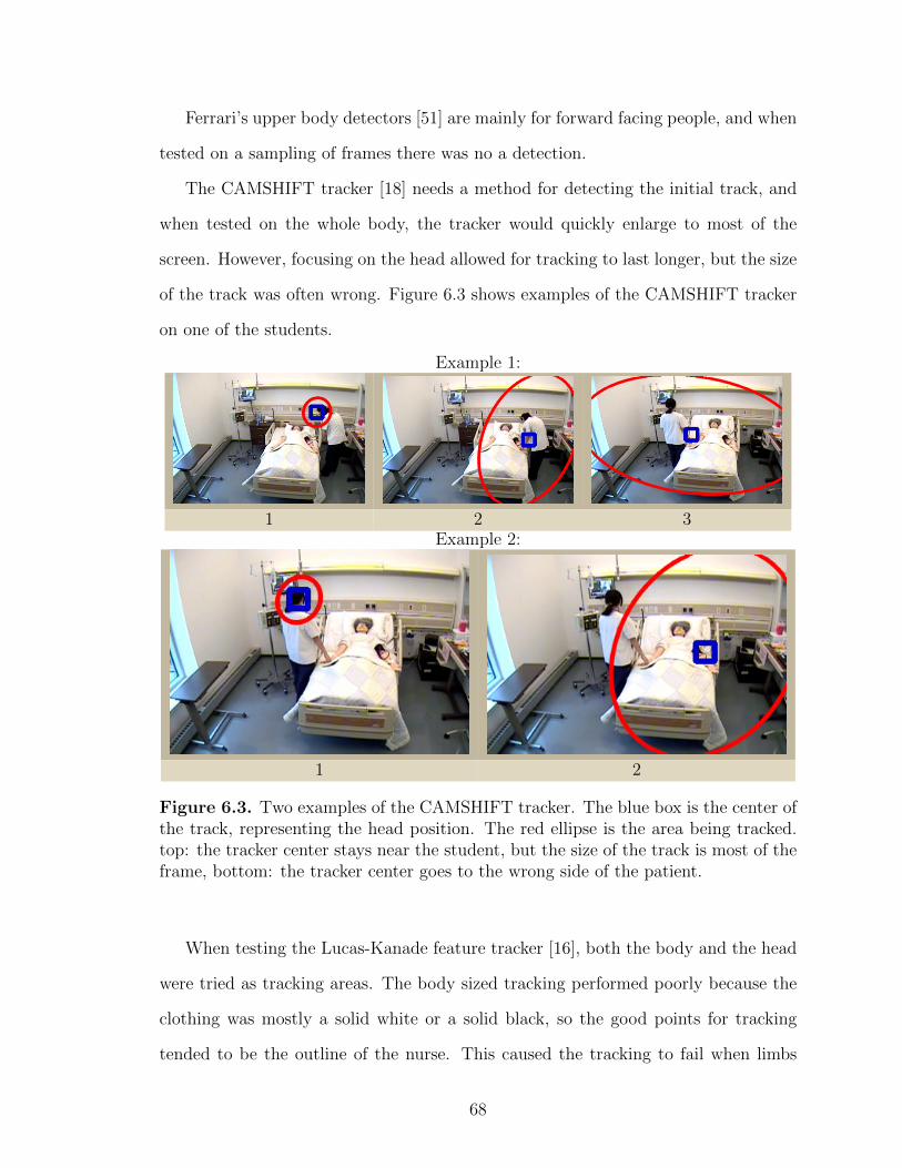
Ferrari’s upper body detectors [51] are mainly for forward facing people, and when
tested on a sampling of frames there was no a detection.
The CAMSHIFT tracker [18] needs a method for detecting the initial track, and
when tested on the whole body, the tracker would quickly enlarge to most of the
screen. However, focusing on the head allowed for tracking to last longer, but the size
of the track was often wrong. Figure 6.3 shows examples of the CAMSHIFT tracker
on one of the students.
Example 1:
1 2 3Example 2:
1 2
Figure 6.3. Two examples of the CAMSHIFT tracker. The blue box is the center ofthe track, representing the head position. The red ellipse is the area being tracked.top: the tracker center stays near the student, but the size of the track is most of theframe, bottom: the tracker center goes to the wrong side of the patient.
When testing the Lucas-Kanade feature tracker [16], both the body and the head
were tried as tracking areas. The body sized tracking performed poorly because the
clothing was mostly a solid white or a solid black, so the good points for tracking
tended to be the outline of the nurse. This caused the tracking to fail when limbs
68
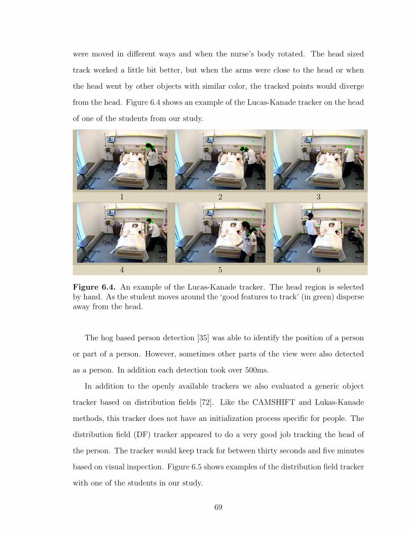
were moved in different ways and when the nurse’s body rotated. The head sized
track worked a little bit better, but when the arms were close to the head or when
the head went by other objects with similar color, the tracked points would diverge
from the head. Figure 6.4 shows an example of the Lucas-Kanade tracker on the head
of one of the students from our study.
1 2 3
4 5 6
Figure 6.4. An example of the Lucas-Kanade tracker. The head region is selectedby hand. As the student moves around the ‘good features to track’ (in green) disperseaway from the head.
The hog based person detection [35] was able to identify the position of a person
or part of a person. However, sometimes other parts of the view were also detected
as a person. In addition each detection took over 500ms.
In addition to the openly available trackers we also evaluated a generic object
tracker based on distribution fields [72]. Like the CAMSHIFT and Lukas-Kanade
methods, this tracker does not have an initialization process specific for people. The
distribution field (DF) tracker appeared to do a very good job tracking the head of
the person. The tracker would keep track for between thirty seconds and five minutes
based on visual inspection. Figure 6.5 shows examples of the distribution field tracker
with one of the students in our study.
69
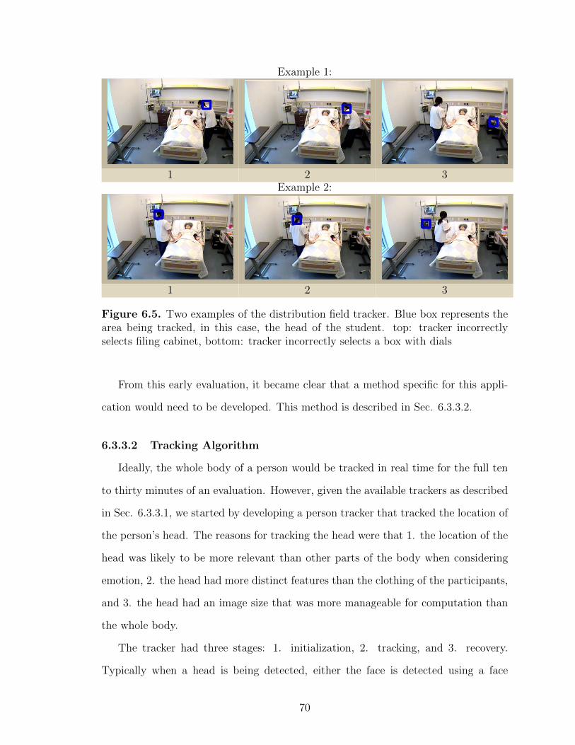
Example 1:
1 2 3Example 2:
1 2 3
Figure 6.5. Two examples of the distribution field tracker. Blue box represents thearea being tracked, in this case, the head of the student. top: tracker incorrectlyselects filing cabinet, bottom: tracker incorrectly selects a box with dials
From this early evaluation, it became clear that a method specific for this appli-
cation would need to be developed. This method is described in Sec. 6.3.3.2.
6.3.3.2 Tracking Algorithm
Ideally, the whole body of a person would be tracked in real time for the full ten
to thirty minutes of an evaluation. However, given the available trackers as described
in Sec. 6.3.3.1, we started by developing a person tracker that tracked the location of
the person’s head. The reasons for tracking the head were that 1. the location of the
head was likely to be more relevant than other parts of the body when considering
emotion, 2. the head had more distinct features than the clothing of the participants,
and 3. the head had an image size that was more manageable for computation than
the whole body.
The tracker had three stages: 1. initialization, 2. tracking, and 3. recovery.
Typically when a head is being detected, either the face is detected using a face
70

detection algorithm, or the head is detected because it is on top of a body. We used
an approximation of the latter approach. For initialization we used a background
subtraction algorithm to get an estimate of the foreground, and then we used a
heuristic that the head was on the part of the highest foreground image that was at
least 75% of the size of the track. We set the size of the track to be 40 x 40 on a
640x480 frame, and we scaled the size down proportionally on a smaller frame size.
The track was initialized by centering the track at the top of the foreground contour
that was selected.
The tracking system was designed such that it can swap in and out different
tracking algorithms. For this study we compare four different tracking algorithms
with a variety of system parameters. We compare two versions of a distribution
field (DF) tracker, the CAMSHIFT tracker, and no tracker (i.e. just continuous
initialization).
Recovery was done by first detecting that the track was lost. A lost track is
defined as a track that does not overlap at all with any foreground contour that is
at least 75% of the head height and width. Once the track is determined to be lost,
one or more potential track positions are determined by searching the foreground for
contours that are big enough to contain a head, and then the tracker searches for the
track from each of those positions, and chooses the best match.
The base algorithm uses the McFarlane and Schofield’s background subtraction
(BGS) method [81] in order to get an estimate of the foreground. The BGS method
was originally intended for tracking piglets and implemented by Parks [93]. This
method of background subtraction is based on adaptive median threshold, and, upon
visual inspection, it did the best job of creating silhouettes of student nurses while
also adapting to the changing position of the patient’s bed. The drawback of this
method is that when an object or person stops for a prolonged amount of time and
71

then moves again, there is an afterglow or ghost of where the person was standing in
addition to the actual foreground silhouette.
Once the foreground is estimated, objects are segregated by the OpenCV [17] im-
plementation of Suzuki and Abe’s border following algorithm [122]. For initialization,
the system chooses the candidate head as the object with a top closest to the top of
the frame, and with a size of at least 75% of the size of a track. If the top of the
candidate head is at or above 60% of the height of the frame, then the candidate
head position is given to the tracker for initialization. At each time step, the track
is compared to the foreground to make sure that the track is not lost. If the track is
lost, then the system gives the tracker one or more starting points for regaining the
track, and tracking continues.
This algorithm is summarized below in pseudocode.
Algorithm 1: Track Nurse
1. head = nil
2. for each frame
(a) do background subtraction
(b) get contours
(c) if no head
head = initialize track
(d) else
lost = track(head)
(e) if lost
head = regain
The initial implementation of this system used the DF tracker, and did not detect
whether the track was lost. It worked well for the first few minutes of one of the
videos, but then it would get stuck on a stationary point for a long time and often
72

would never regain the track because the tracker had no way of knowing that the
track was lost.
For comparison, the CAMSHIFT tracker from OpenCV was also used for the track
and regain steps. Since our algorithm expects the track to remain the same size, the
CAMSHIFT tracker is constrained to the initial patch size by centering the patch
bounds of the reported track on the CAMSHIFT track regardless of the size of the
CAMSHIFT track.
Once the ability to detect a lost track exists, there are a number of ways to regain
the track. One is to delete all of the information about the track, then initialize a
new track, and another way is to save the model of the track in order to regain the
track with the learned appearance model of the track.
In addition, there are other ways that the foreground of the track may be helpful
to both the tracker and the BGS method. These are described next.
6.3.3.3 Tracking algorithm variants
6.3.3.3.1 Variant 1a: Foreground distance The DF tracker computes the L1
distance between the stored model track and the distribution field of the predicted
position. One way to augment the tracker is to include a foreground/background
model as part of the track so that in addition to comparing the distribution fields,
the foreground mask of the predicted position can be compared to the foreground
mask model of the track. This modification requires an additional storage of the
foreground mask model that is track width by track height in dimension stored as
doubles in order to allow the model to be updated over time.
We initialize a foreground mask, fm from the detected foreground, F , in a patch
such that
fm(i, j) =
1 if F (i, j) = TRUE,
0 if F (i, j) = FALSE,(6.1)
73

for all pairs i, j in the image patch where i and j are row and column indices re-
spectively. The foreground masks are compared by the L1 distance between each
other:
DL1(fm1, fm2) =∑i,j
|fm1(i, j)− fm2(i, j)| . (6.2)
When computing the distance between a potential object o and the model m we
compute
D(m, o) =1
p(αD(dfm, dfo) + βD(fmm, fmo)) , (6.3)
where p is the pixel area of the patch, α and β are mixing parameters. The mixing
parameters are necessary to balance the contribution between the distribution field
distance and the foreground mask distance. The purpose of using a foreground mask
as part of the distance function is so that the shape of the object that is being tracked
is modeled in addition to the rectangular patch in which the object appears. This is
a loose approximation of fine segmentation as described by Aeschliman et al., [1].
6.3.3.3.2 Variant 1b: Foreground masking For the CAMSHIFT tracker, there
is already a mask to remove pixels that are not within a particular hue and satura-
tion range. The foreground prediction can be used as a mask in addition to standard
mask, to prevent the CAMSHIFT track from drifting to background that has a similar
color model to the head. With this variant, there is just an initial step of taking the
intersection of the foreground mask and the CAMSHIFT hue and saturation mask.
6.3.3.3.3 Variant 2: Multiple candidates When tracking, the standard DF
tracker predicts the location of the next track based on a motion estimate, and then
it searches for the object based on a gradient descent of the distance. The object
position is determined by the minimum distance between the model’s distribution
field and the potential object’s distribution field.
By using the foreground contours, in addition to the predicted object’s position
as a candidate for gradient descent, other candidates are selected by finding potential
74

heads (i.e. contours that are at least 75% of the track size), and extracting a patch
that is centered at the top of the contour. Then the multiple candidates are used
for the gradient descent search, and the basin with the lowest distance will be the
tracked position.
By having multiple candidates, the tracker may be able to recover from quick
changes in velocity.
6.3.3.3.4 Variant 3: Track based conditional background updates By de-
fault, when the BGS algorithm updates its background model, the entire frame is
used to update the model. However, there is the option to pass in a foreground mask
that will not update the model. This variant of our tracker selects every foreground
contour that the track overlaps with, and adds these contours to the foreground mask
that is passed to the BGS algorithm. If the track is tracking correctly, then this
should remove the ghosting problems that occur when a person stays in one place for
a long time.
6.3.3.3.5 Variant 4: Re-initialize instead of regain tracks en a track is
lost, there is a potential that the model for the track has been corrupted due to
misalignment with the track. If this is the case, then the process of regaining the
track could potentially choose the wrong candidate head. One way to mitigate this
problem is to re-initialize the track based on the initialization heuristic. The pro for
this approach is that the model does not have corrupted data. The con is that the
initialization could choose the wrong position, and then the model would not just be
corrupted, but would be altogether bad. Though, this variant may not be an ideal
solution, it is very easy to implement and compare.
75
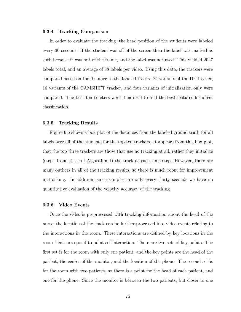
6.3.4 Tracking Comparison
In order to evaluate the tracking, the head position of the students were labeled
every 30 seconds. If the student was off of the screen then the label was marked as
such because it was out of the frame, and the label was not used. This yielded 2027
labels total, and an average of 38 labels per video. Using this data, the trackers were
compared based on the distance to the labeled tracks. 24 variants of the DF tracker,
16 variants of the CAMSHIFT tracker, and four variants of initialization only were
compared. The best ten trackers were then used to find the best features for affect
classification.
6.3.5 Tracking Results
Figure 6.6 shows a box plot of the distances from the labeled ground truth for all
labels over all of the students for the top ten trackers. It appears from this box plot,
that the top three trackers are those that use no tracking at all, rather they initialize
(steps 1 and 2 a-c of Algorithm 1) the track at each time step. However, there are
many outliers in all of the tracking results, so there is much room for improvement
in tracking. In addition, since samples are only every thirty seconds we have no
quantitative evaluation of the velocity accuracy of the tracking.
6.3.6 Video Events
Once the video is preprocessed with tracking information about the head of the
nurse, the location of the track can be further processed into video events relating to
the interactions in the room. These interactions are defined by key locations in the
room that correspond to points of interaction. There are two sets of key points. The
first set is for the room with only one patient, and the key points are the head of the
patient, the center of the monitor, and the location of the phone. The second set is
for the room with two patients, so there is a point for the head of each patient, and
one for the phone. Since the monitor is between the two patients, but closer to one
76
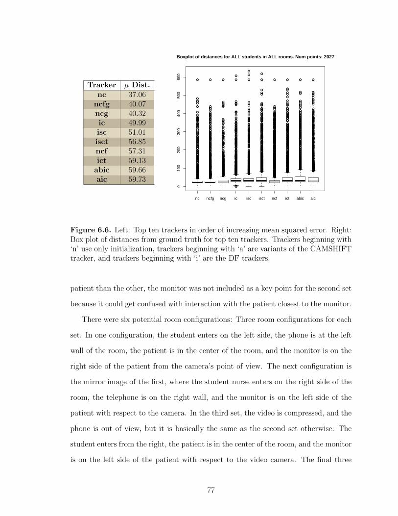
Tracker µ Dist.nc 37.06
ncfg 40.07ncg 40.32ic 49.99isc 51.01isct 56.85ncf 57.31ict 59.13
abic 59.66aic 59.73
●
●
●
●
●
●
●●
●
●
●
●
●
●
●
●
●
●
●
●
●
●
●
●
●●●
●●
●
●●
●
●
●
●●
●
●●●●
●●●
●
●●
●
●●
●
●●●●
●●●
●
●
●
●
●●
●
●
●●
●
●
●
●●
●
●
●
●
●
●
●
●
●
●
●●
●●
●
●
●
●
●
●
●
●●●
●
●
●●●
●
●
●
●
●
●
●
●
●
●●●●●
●
●
●
●
●
●
●
●
●
●
●
●
●
●
●
●●
●●
●
●
●
●
●
●
●
●
●
●
●
●
●
●
●
●
●●
●
●●
●
●
●
●
●
●●●
●
●●
●●●
●●
●
●
●
●
●
●
●●
●
●
●
●
●
●●
●
●
●●●
●
●
●
●●
●
●
●
●
●
●
●●
●●
●●●
●
●
●●
●
●
●
●
●
●
●
●
●
●
●●
●
●●
●●
●
●
●
●
●
●
●
●●
●
●●
●
●
●
●
●●●
●
●
●
●●
●
●
●
●
●
●
●
●
●
●●
●
●
●
●●●
●
●
●●
●
●
●
●●●●●
●
●
●
●
●
●
●
●
●
●●●
●
●
●
●●
●
●
●
●
●
●●
●●
●
●
●
●
●
●●●
●●
●
●
●
●●
●
●
●
●
●
●
●
●
●
●
●●
●
●
●●
●
●
●●
●
●●
●
●
●
●●
●
●
●●●
●
●
●●
●
●
●
●
●
●
●
●
●
●
●
●
●●
●
●
●●
●●
●
●●
●
●
●
●
●
●
●
●
●
●
●
●
●
●
●
●
●●
●
●
●
●
●●
●
●
●
●
●
●
●
●
●●
●●●
●●
●
●
●
●●
●
●●●
●
●
●
●
●
●
●
●●
●
●
●●●●●●●
●
●
●●
●
●
●
●
●
●●
●
●
●
●
●
●
●●●
●
●●
●
●
●●●
●
●
●
●
●
●
●
●
●
●
●
●
●
●●●
●
●●
●
●●
●●●
●
●
●
●
●
●●
●
●
●
●
●
●
●●
●
●
●●
●
●●
●
●●●
●
●
●
●●
●
●
●
●
●
●
●
●●
●●
●
●●
●
●
●
●
●
●
●
●
●●●
●
●●●
●
●●●●●●
●
●
●
●
●
●●
●●●●●
●
●
●
●
●
●●
●
●●●
●
●
●
●
●
●●
●
●
●
●
●
●●●
●
●
●
●●
●
●
●●
●
●
●
●
●●●●
●●
●
●
●
●
●
●
●
●
●●
●
●
●●
●●●
●●
●●
●
●
●●●
●
●
●
●
●
●
●
●
●
●
●
●
●●
●●
●
●
●
●
●
●
●
●
●
●
●
●
●
●●
●
●
●
●
●
●
●
●
●
●●●●
●●
●
●
●
●●
●
●
●●●
●●
●
●
●
●●
●
●●●
●
●●●●●●
●
●●●●●●●●●
●
●
●
●
●
●
●●●
●
●
●●●
●
●
●
●
●
●
●
●
●
●
●
●
●
●
●●●
●
●●
●
●
●
●
●●
●
●
●
●
●
●
●
●●●
●
●
●●
●●
●●●●
●
●
●●●
●
●
●
●
●●●●●
●
●
●●●
●
●
●
●
●
●
●
●
●
●
●
●
●
●
●
●
●
●
●
●
●
●
●
●
●●●
●
●
●
●
●
●
●●●●
●
●
●
●
●
●●
●●●●
●
●●●
●
●
●
●
●
●
●
●●
●
●
●
●
●●
●
●
●
●
●
●
●●●●
●
●
●
●
●
●
●
●
●
●●
●
●●●
●
●●
●
●
●
●
●
●
●
●
●
●
●
●
●
●
●
●
●
●●
●●●●
●
●●
●
●●
●
●
●
●
●
●
●
●●
●
●●
●
●
●
●
●
●
●
●●
●
●
●
●
●●
●
●
●
●
●
●
●
●
●
●
●
●
●
●
●
●
●
●
●
●●
●
●●
●●
●
●
●
●
●
●
●
●
●●
●
●
●
●
●●
●
●
●
●●●
●
●
●
●
●
●
●
●
●
●
●
●
●
●
●
●●●
●●
●
●
●
●
●
●
●
●
●
●
●
●
●
●
●
●
●●
●
●
●
●
●
●●
●
●
●
●●
●
●
●
●●
●
●
●
●●
●
●
●
●
●●
●●
●
●●
●
●
●
●
●
●
●
●
●●●●●●
●
●
●
●●●●
●
●
●
●
●
●
●
●
●
●
●
●
●
●
●
●
●
●
●
●
●●
●
●●
●
●●●
●
●
●●
●
●
●
●●
●
●●
●
●
●●●
●
●
●
●
●
●
●
●
●●●
●●
●
●
●
●
●
●
●
●
●
●
●
●●
●
●
●
●
●●
●
●
●
●
●
●
●
●
●
●
●
●●
●●
●●
●
●
●
●
●
●
●
●
●
●
●
●
●
●●●●
●
●●●●
●
●
●●
●
●
●●
●●
●
●
●●
●
●●
●
●●●
●●
●
●●
●●
●●
●
●
●
●●
●●●
●
●
●
●
●
●
●
●
●
●
●
●
●●
●
●
●●
●
●
●●
●
●
●
●
●●
●
●●
●
●
●
●●
●
●
●
●●
●
●
●
●
●●
●
●
●
●
●
●●
●
●
●
●
●
●
●
●●●
●
●
●●
●
●
●
●
●●
●
●
●
●
●●
●
●
●
●●
●
●
●
●
●
●
●
●
●●
●
●●
●
●
●
●
●●
●●
●
●
●
●●
●●
●
●
●●
●●
●
●●●
●
●
●
●
●
●
●
●●●
●
●
●
●
●
●
●●
●
●●
●
●
●
●
●
●●
●
●
●
●
●
●
●
●●
●●●
●
●●
●
●
●
●
●
●●
●
●
●●
●
●
●
●
●●
●
●
●
●
●
●●●●●●
●●
●
●
●
●
●
●
●
●
●
●
●
●
●
●
●
●
●
●
●
●
●
●
●
●
●
●
●●●
●
●
●●
●
●
●●
●
●
●●
●
●
●
●
●
●
●
●
●●
●●●
●
●
●●
●
●
●●
●
●
●
●
●
●●
●●
●
●
●
●
●●
●
●●
●
●
●
●●
●
●●
●●●
●
●
●
●
●
●
●
●
●
●
●
●
●
●
●
●
●
●
●
●
●
●
●
●
●●
●
●
●
●●●
●
●●
●
●
●
●●
●●
●
●●
●
●●●●●●●
●●●●
●
●
●●
●●●
●
●
●
●
●
●
●
●●
●
●
●
●
●
●
●
●
●
●
●
●
●●
●
●
●
●
●
●
●
●
●●
●
●
●
●
●
●
●
●
●
●●●●
●
●●
●
●●
●
●
●
●
●
●
●
●
●
●
●●
●●
●
●
●
●
●
●
●●●
●
●
●
●
●
●
●
●
●
●
●●
●
●
●●●
●
●
●
●
●
●●
●
●
●
●
●
●
●
●
●
●
●
●
●
●●
●
●
●
●
●
●●
●●
●
●
●
●
●
●
●
●
●
●●
●
●●
●●
●
●
●
●
●
●●●
●●
●
●
●
●
●
●
●
●
●
●
●
●●●
●●
●
●
●
●
●
●
●
●●
●
●
●●
●●
●●
●
●
●
●
●
●
●●
●
●●
●●
●
●●
●
●
●●
●
●●
●
●
●
●●
●●
●
●
●
●
●
●
●
●●
●
●
●
●
●
●
●
●
●
●
●
●
●
●●●●●
●
●
●●
●
●
●●
●
●
●
●●●
●
●
●
●●
●
●
●
●
●
●
●
●●
●
●
●
●●●
●
●
●
●●
●
●●
●●●
●
●
●
●
●
●●
●
●
●●●
●
●●●
●●
●●
●
●
●●
●
●
●
●
●●
●
●●
●●
●
●
●
●
●
●
●
●
●
●
●
●●
●
●
●●
●●
●
●
●●●●
●
●
●
●
●
●
●
●
●
●
●
●
●●
●●
●
●
●
●
●
●
●
●
●
●
●
●
●
●
●
●
●●
●
●
●
●
●●
●
●
●
●
●
●
●
●
●●
●●●
●●
●
●
●
●
●
●
●
●
●
●●
●
●●●
●
●
●
●
●
●
●●●●
●
●
●
●
●
●
●
●
●
●
●
●●
●
●
●
●
●
●
●
●
●
●●●
●
●
●
●
●
●
●
●
●
●
●
●●●●
●
●
●●●●
●
●
●
●
●
●
●●
●
●●
●●
●
●
●
●●
●
●●
●
●●
●
●
●
●●
●●
●
●
●
●
●
●
●
●
●
●●
●
●
●
●
●●
●
●
●
●
●
●
●
●
●
●
●
●
●
●
●
●
●●
●
●
●
●
●
●
●
●
●
●●
●●●●
●
●
●●●●
●●
●
●
●●
●●
●
●
●
●
●
●
●
●
●●
●
●
●
●
●
●●
●●
●
●●
●●
●
●
●
●
●
●
●●
●
●
●
●
●
●
●
●
●
●
●
●
●
●
●●
●
●
●
●
●
●
●
●
●
●
●
●
●
●
●
●●
●
●
●
●
●
●
●
●
●
●
●
●
●
●
●
●●
●
●
●●
●●
●●●
●●
●●●
●
●
●
●
●●
●
●
●
●
●
●
●●
●●
●
●●
●
●
●
●
●
●
●●
●
●
●
●
●
●
●
●
●
●
●
●
●
●●
●
●●
●
●
●●
●
●●
●
●
●
●
●
●●
●
●
●●
●
●
●
●
●
●●●
●
●
●
●
●
●
●
●
●
●
●
●●
●
●
●
●●
●
●
●
●
●
●●●
●
●
●
●
●
●
●
●
●●
●
●
●
●
●
●
●
●
●
●
●
●
●
●
●
●
●
●
●
●
●
●●
●
●
●
●
●
●
●
●●
●
●
●
●●
●
●
●
●●
●
●
●
●●
●
●
●
●
●
●
●
●
●●
●
●
●
●
●
●
●
●●
●
●
●
●
●
●
●
●
●
●●
●
●
●
●●
●
●
●
●
●
●
●
●
●●
●
●
●
●
●
●
●
●
●
●
●
●
●
●
●
●
●
●
●
●
●
●
●●
●
●
●●
●●
●
●●
●
●
●
●
●●●●
●
●
●
●
●
●
●●●
●
●●
●
●
●
●
●
●
●
●
●
●
●
●
●
●
●
●
●
●
●
●
●
●
●
●
●
●
●
●
●
●
●
●
●
●
●
●
●
●
●
●
●●
●●
●
●
●
●
●
●●
●
●
●
●●
●
●
●
●
●
●
●
●
●
●
●
●
●
●●●
●●
●●
●●
●
●
●
●
●
●
●●
●●
●
●
●
●
●
●
●
●
●
●
●
●
●
●●
●
●●●●●
●
●
●
●
●●●
●
●●
●
●
●
●
●●●
●
●●
●
●
●
●
●●
●●
●
●
●●
●
●●
●
●●
●
●
●
●
●
●
●
●
●
●
●
●
●
●
●
●●
●●
●
●
●
●
●
●
●
●
●●
●
●
●
●●
●
●
●●●
●
●
●●●●●●●●
●●
●
●●
●
●
●
●
●●●
●
●
●
●
●●
●●
●
●
●
●
●
●
●
●
●
●
●
●
●
●●
●
●
●
●
●●
●
●
●
●
●
●●
●●
●
●
●
●
●
●
●
●
●●
●
●
●
●
●
●
●
●
●
●
●
●
●●
●
●
●●
●
●●
●
●●
●●●
●
●●
●●
●
●
●●
●
●
●
●
●●
●
●
●
●
●
●
●
●
●
●
●
●
●
●
●
●
●
●
●
●
●
●
●
●
●
●
●●●
●
●
●
●
●●
●
●
●
●
●●
●
●
●●
●●
●●
●●●
●
●
●
●●●
●
●
●
●●
●●
●
●
●
●
●
●
●●
●
●
●
●
●
●
●
●
●
●
●
●●
●
●
●
●
●
●
●
●●●●
●●●
●
●
●
●
●
●●
●
●
●
●
●●
●
●
●
●
●
●●
●
●●●
●
●
●
●●●
●
●
●
●●
●●
●
●
●●●●●●●
●
●
●
●
●
●●●
●
●
●●
●
●
●
●
●
●
●
●
●
●
●
●
●
●
●
●
●
●
●
●●
nc ncfg ncg ic isc isct ncf ict abic aic
010
020
030
040
050
060
0
Boxplot of distances for ALL students in ALL rooms. Num points: 2027
Figure 6.6. Left: Top ten trackers in order of increasing mean squared error. Right:Box plot of distances from ground truth for top ten trackers. Trackers beginning with‘n’ use only initialization, trackers beginning with ‘a’ are variants of the CAMSHIFTtracker, and trackers beginning with ‘i’ are the DF trackers.
patient than the other, the monitor was not included as a key point for the second set
because it could get confused with interaction with the patient closest to the monitor.
There were six potential room configurations: Three room configurations for each
set. In one configuration, the student enters on the left side, the phone is at the left
wall of the room, the patient is in the center of the room, and the monitor is on the
right side of the patient from the camera’s point of view. The next configuration is
the mirror image of the first, where the student nurse enters on the right side of the
room, the telephone is on the right wall, and the monitor is on the left side of the
patient with respect to the camera. In the third set, the video is compressed, and the
phone is out of view, but it is basically the same as the second set otherwise: The
student enters from the right, the patient is in the center of the room, and the monitor
is on the left side of the patient with respect to the video camera. The final three
77
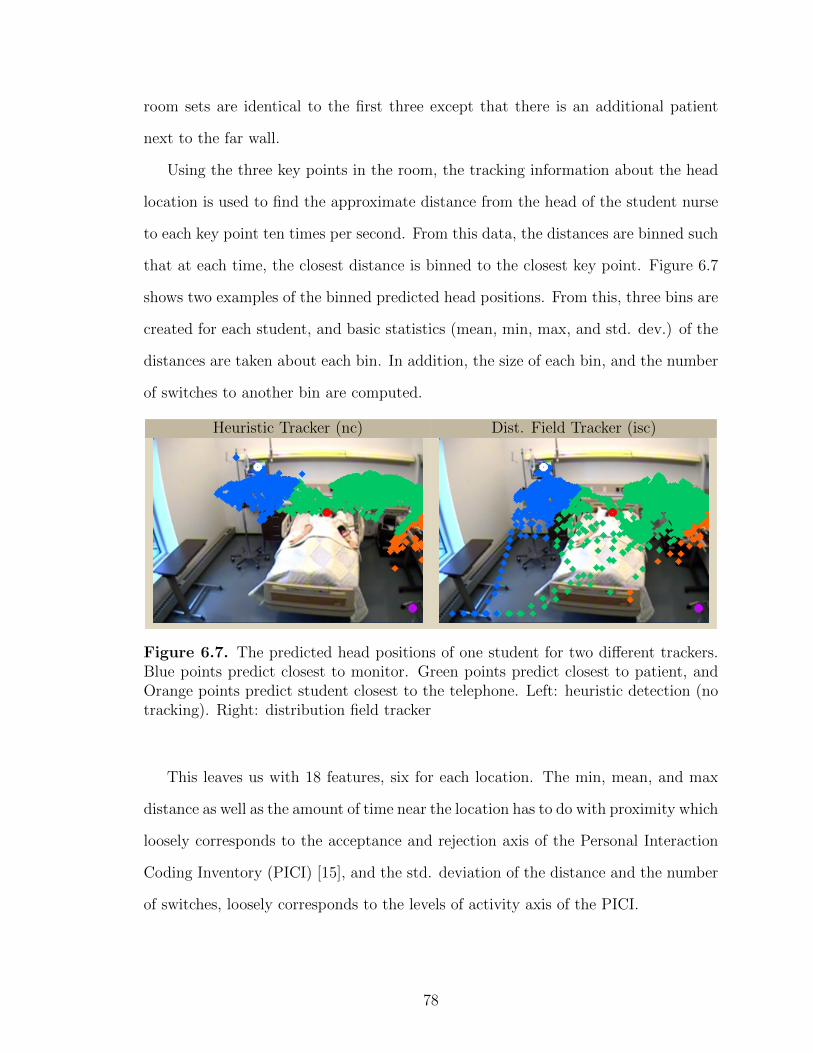
room sets are identical to the first three except that there is an additional patient
next to the far wall.
Using the three key points in the room, the tracking information about the head
location is used to find the approximate distance from the head of the student nurse
to each key point ten times per second. From this data, the distances are binned such
that at each time, the closest distance is binned to the closest key point. Figure 6.7
shows two examples of the binned predicted head positions. From this, three bins are
created for each student, and basic statistics (mean, min, max, and std. dev.) of the
distances are taken about each bin. In addition, the size of each bin, and the number
of switches to another bin are computed.
Heuristic Tracker (nc) Dist. Field Tracker (isc)
Figure 6.7. The predicted head positions of one student for two different trackers.Blue points predict closest to monitor. Green points predict closest to patient, andOrange points predict student closest to the telephone. Left: heuristic detection (notracking). Right: distribution field tracker
This leaves us with 18 features, six for each location. The min, mean, and max
distance as well as the amount of time near the location has to do with proximity which
loosely corresponds to the acceptance and rejection axis of the Personal Interaction
Coding Inventory (PICI) [15], and the std. deviation of the distance and the number
of switches, loosely corresponds to the levels of activity axis of the PICI.
78
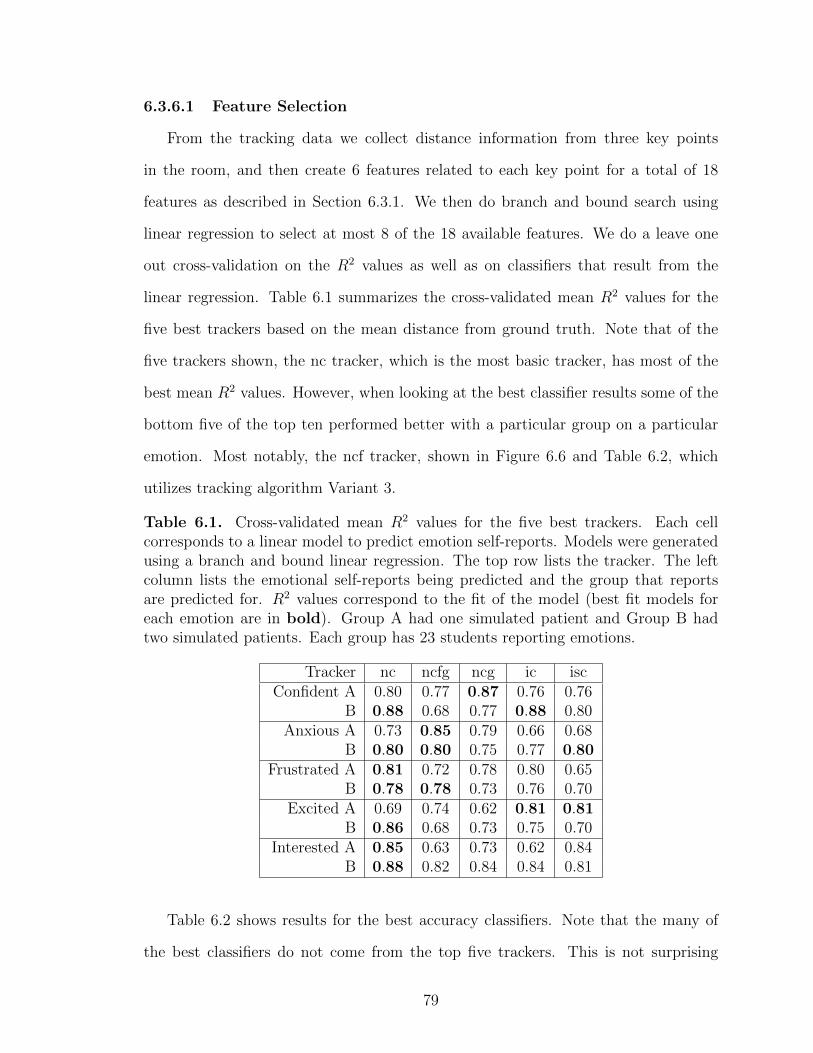
6.3.6.1 Feature Selection
From the tracking data we collect distance information from three key points
in the room, and then create 6 features related to each key point for a total of 18
features as described in Section 6.3.1. We then do branch and bound search using
linear regression to select at most 8 of the 18 available features. We do a leave one
out cross-validation on the R2 values as well as on classifiers that result from the
linear regression. Table 6.1 summarizes the cross-validated mean R2 values for the
five best trackers based on the mean distance from ground truth. Note that of the
five trackers shown, the nc tracker, which is the most basic tracker, has most of the
best mean R2 values. However, when looking at the best classifier results some of the
bottom five of the top ten performed better with a particular group on a particular
emotion. Most notably, the ncf tracker, shown in Figure 6.6 and Table 6.2, which
utilizes tracking algorithm Variant 3.
Table 6.1. Cross-validated mean R2 values for the five best trackers. Each cellcorresponds to a linear model to predict emotion self-reports. Models were generatedusing a branch and bound linear regression. The top row lists the tracker. The leftcolumn lists the emotional self-reports being predicted and the group that reportsare predicted for. R2 values correspond to the fit of the model (best fit models foreach emotion are in bold). Group A had one simulated patient and Group B hadtwo simulated patients. Each group has 23 students reporting emotions.
Tracker nc ncfg ncg ic iscConfident A 0.80 0.77 0.87 0.76 0.76
B 0.88 0.68 0.77 0.88 0.80Anxious A 0.73 0.85 0.79 0.66 0.68
B 0.80 0.80 0.75 0.77 0.80Frustrated A 0.81 0.72 0.78 0.80 0.65
B 0.78 0.78 0.73 0.76 0.70Excited A 0.69 0.74 0.62 0.81 0.81
B 0.86 0.68 0.73 0.75 0.70Interested A 0.85 0.63 0.73 0.62 0.84
B 0.88 0.82 0.84 0.84 0.81
Table 6.2 shows results for the best accuracy classifiers. Note that the many of
the best classifiers do not come from the top five trackers. This is not surprising
79
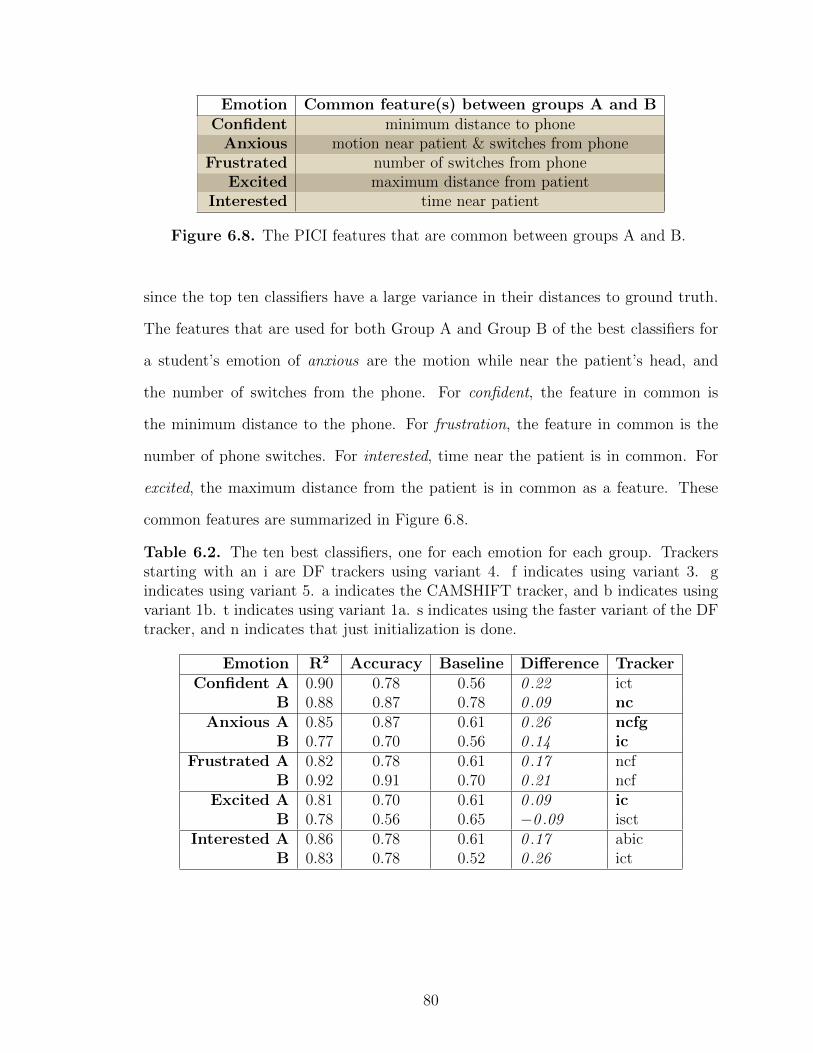
Emotion Common feature(s) between groups A and BConfident minimum distance to phone
Anxious motion near patient & switches from phoneFrustrated number of switches from phone
Excited maximum distance from patientInterested time near patient
Figure 6.8. The PICI features that are common between groups A and B.
since the top ten classifiers have a large variance in their distances to ground truth.
The features that are used for both Group A and Group B of the best classifiers for
a student’s emotion of anxious are the motion while near the patient’s head, and
the number of switches from the phone. For confident, the feature in common is
the minimum distance to the phone. For frustration, the feature in common is the
number of phone switches. For interested, time near the patient is in common. For
excited, the maximum distance from the patient is in common as a feature. These
common features are summarized in Figure 6.8.
Table 6.2. The ten best classifiers, one for each emotion for each group. Trackersstarting with an i are DF trackers using variant 4. f indicates using variant 3. gindicates using variant 5. a indicates the CAMSHIFT tracker, and b indicates usingvariant 1b. t indicates using variant 1a. s indicates using the faster variant of the DFtracker, and n indicates that just initialization is done.
Emotion R2 Accuracy Baseline Difference TrackerConfident A 0.90 0.78 0.56 0 .22 ict
B 0.88 0.87 0.78 0 .09 ncAnxious A 0.85 0.87 0.61 0 .26 ncfg
B 0.77 0.70 0.56 0 .14 icFrustrated A 0.82 0.78 0.61 0 .17 ncf
B 0.92 0.91 0.70 0 .21 ncfExcited A 0.81 0.70 0.61 0 .09 ic
B 0.78 0.56 0.65 −0 .09 isctInterested A 0.86 0.78 0.61 0 .17 abic
B 0.83 0.78 0.52 0 .26 ict
80
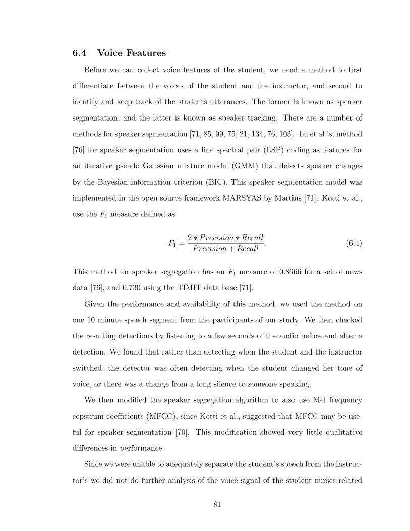
6.4 Voice Features
Before we can collect voice features of the student, we need a method to first
differentiate between the voices of the student and the instructor, and second to
identify and keep track of the students utterances. The former is known as speaker
segmentation, and the latter is known as speaker tracking. There are a number of
methods for speaker segmentation [71, 85, 99, 75, 21, 134, 76, 103]. Lu et al.’s, method
[76] for speaker segmentation uses a line spectral pair (LSP) coding as features for
an iterative pseudo Gaussian mixture model (GMM) that detects speaker changes
by the Bayesian information criterion (BIC). This speaker segmentation model was
implemented in the open source framework MARSYAS by Martins [71]. Kotti et al.,
use the F1 measure defined as
F1 =2 ∗ Precision ∗RecallPrecision+Recall
. (6.4)
This method for speaker segregation has an F1 measure of 0.8666 for a set of news
data [76], and 0.730 using the TIMIT data base [71].
Given the performance and availability of this method, we used the method on
one 10 minute speech segment from the participants of our study. We then checked
the resulting detections by listening to a few seconds of the audio before and after a
detection. We found that rather than detecting when the student and the instructor
switched, the detector was often detecting when the student changed her tone of
voice, or there was a change from a long silence to someone speaking.
We then modified the speaker segregation algorithm to also use Mel frequency
cepstrum coefficients (MFCC), since Kotti et al., suggested that MFCC may be use-
ful for speaker segmentation [70]. This modification showed very little qualitative
differences in performance.
Since we were unable to adequately separate the student’s speech from the instruc-
tor’s we did not do further analysis of the voice signal of the student nurses related
81
to their self-reported emotions. Though the majority of the speech is the student
nurse’s, it is unclear at this time how much the features would be corrupted by the
instructor’s voice.
6.4.1 Future work
There are a number of directions that the voice analysis could go. Ideally an
automatic method can be created for separating the student’s speech from the in-
structor’s speech. Without that, the speech data could be extracted by a human.
Once the data is separated, then the methods described in Section 5.3 could be used
on the emotional labels used for the video classification in Section 6.3.2. In addition,
extracting audio events based on extracted video events such as close proximity to a
patient, may be a very effective method of finding salient affective features.
6.5 Discussion & Future Work
Detecting the emotions of people as they interact with their environment has
many potential applications. This study indicates that simple motion cues relative
to key interaction points may be enough to computationally assess the affective state
of a person. This study also identifies some limitations of current real-time trackers.
There is a lot of room for improvement so that a tracker can track the head more
closely, and recover better from when the location of the head is lost.
In addition, the potential exists to use the time series of the data rather than just
basic statistics over the entire session. Once tracking is better, it would be interesting
to see if more gestural information could be captured from the foreground contours.
This may require much higher fidelity labeling of the data.
Labeling the head position every half minute allowed us to validate how well
the trackers were doing at various check points, but labeling every half second (or
82

even every frame) would be preferred. This would be an ideal application for crowd
sourcing, however, it would be difficult to keep the privacy of the participants.
One place for future work is to run a follow-up study with multiple schools of
nursing that have a similar setup. This way we can recruit a larger participant pool
to verify our results.
83

CHAPTER 7
DISCUSSION AND FUTURE WORK
7.1 Hypotheses Revisited
1. Sensors can effectively augment tutor logs in order to predict the self-reported
emotions of students.
True. The linear least square regression results from Chapter 3 indicate that
sensors do indeed improve the prediction quality of self-reported emotions
for all four of the emotions in question confident, frustrated, excited, and
interested, as shown in Table 3.3.
2. Linear least squares classifiers built from the tutor and sensor data can predict
high vs. low levels of frustration, confidence, interest, and excitement.
Mixed. This hypothesis held true for confident, excited, and interested, but
it was false for frustrated. We were unable to use a linear least squares
classifier for frustrated that was significantly better than using no classifier
at all.
3. The accuracy, specificity, and/or sensitivity of the frustration, confidence, inter-
est, and excitement classifiers that use tutor and/or sensor features will continue
to perform significantly better than the baseline classifier for the given emotion
on a novel population.
Mixed. This held true for specificity results for confidence. It also held true for
sensitivity results for interest and excitement. However, overall accuracy
was not held up for any of the four emotions.
84

4. The method of feature selection and linear least squares classification will trans-
fer to the voice domain.
Mixed For the two class problems, such as gender and American vs. Asian
voices, the method shows better than baseline performance, however, the
method appears to be insufficient for the multi-class problem of multiple
cultures in voice.
5. Low confidence is correlated with high anxiety in learning situations.
True. When comparing levels of self-reported confidence and anxiety about
the student’s test in the health care education experiment, the correlation
test showed a high negative correlation using Pearson’s product moment
correlation test: r = −0.632, t = −5.48, df = 45, p-value= 9.235e − 07,
with a 95% confidence interval of [-1.0,-0.46]. This is strong evidence that
there is a high correlation between low confidence and high anxiety in
learning situations.
6. Available methods for real-time people tracking are adequate for tracking the
nurses in the video.
Mixed. When looking at the results of the tracker comparison in Figure 6.6,
there are clearly a lot of outliers for all of the trackers. This suggests
that there are many cases where the tracker is not correctly tracking the
position of the head of the student. However, the features gleaned from the
tracking predictions were good enough to make classifiers that performed
better than chance.
7. PICI related features in the video will help to predict or classify the self-reported
emotional state of the student.
85

True. We were able to find both motion and proximity related features that
helped classify low and high levels of all five of the emotional states in
question (anxious, confident, excited, frustrated, and interested). Classifier
results of best classifiers are summarized in Table 6.2.
8. Contemporary methods for automatic extraction of audio will be sufficient to
separate the student nurses voice from other sounds and voices in the audio
recording.
False. The available method for speaker segregation is not good enough to ex-
tract the students voice from the other voices and sounds in the recording.
9. Prosodic features will be relevant for emotional change.
Unknown. We could not explore this hypothesis adequately given the nature
of the audio data. Either an automatic speaker segregation algorithm or
hand extraction is needed for this to be tested.
7.2 Lessons Learned and Future Directions
7.2.1 Computer Based Education
7.2.1.1 Sensors
The use of over 100 sensors at a time is a very ambitious endeavor. The research
in Chapters 3 and 4 is just the first step in determining the usefulness of these sensors
for detecting affect in ITS settings. The sensor values that ended up performing well
were those that correlated most with a particular action of the student rather than the
raw sensor values. With that in mind, one next step for future directions may be using
an automatic feature discovery algorithm based on the temporal data. This could be
using time series motif discovery, topic models, hidden Markov models (HMM), or
deep belief networks. We began looking at time series motif discovery for just the
tutor data with some promising results [112], but we have yet to look at the sensor
86

data in that way. We did a preliminary exploration of topic models using the sensor
and tutor data together, however the topics found did not yield good classifiers, and
it was unclear whether we translated the data to documents in the best way. Further
exploration will have to be done before topic modeling should be ruled out.
7.2.1.2 Controls
If we were to run more studies with the sensors in the future, it would be useful to
collect some baseline data with the sensors when the students are doing a sequence of
known activities without problem solving. In this way we can have an idea of the way
that students differ from the norm with a fixed set of activities that can be compared
in a more controlled way. Since we only had data from a hard to control environment,
it was difficult to determine the amount of noise or spurious data there was with the
affective signal.
7.2.1.3 Feedback
Now that we have some idea of how the students are feeling, the next step is to
target our emotional queries so that we can ask about a feeling that is likely to occur.
For instance, if the system detects that the student is anxious, then the question
“How confident are you feeling?” would be displayed to the student. This way we
can improve our classifiers with more relevant data.
7.2.2 Speaker Differences and Health Diagnosis
7.2.2.1 Classifiers
Our research found that for the multi-class problem of differentiating four cultures,
the linear least squares classifier was insufficient. There are a number of other methods
that may work better for this. Linear models such as linear discriminant analysis
(LDA) and logistic regression classifiers are one option. Another option is to use a
k-nearest neighbors technique, which allows for local linear relationships. Support
87

Vector Machines (SVM) can use polynomial or radial basis kernels which may work
better for multi-class problems as well.
7.2.2.2 Categories
In addition to the categories of gender and culture. Using similar computational
methods for categorizing different health conditions such as differentiating typically
developing (TD) children from childhood apraxia of speech (CAS) and autism spec-
trum disorder (ASD) is the logical next step for this work. In addition, directly
evaluating speech from evoked emotions is an important next step.
7.2.3 Heath Care Education
The student nurse pilot study was a very good first step for collecting a data
set for understanding emotion from video and voice. However, there is potential to
increase the quality of future data collection efforts.
7.2.3.1 Controls
One aspect that can be improved is the creation of controlled interaction with
the key points in the room. This could be done by creating a control scenario in the
simulation room with tasks that just involve moving around the room and speaking,
without having to evaluate a patient or talk to a doctor over the phone. By having
each participant enact a script that has little or no emotional charge to it, the par-
ticipants can be compared to themselves in the control condition to determine how
emotional they are being.
There are other controls that were considered, but are both infeasible and un-
desirable in order to maintain ecological validity. These are having a microphone
a fixed distance from the participant at all times, controlling for ambient noise and
other noise sources, and limiting speech to one speaker at a time. Rather than control
for these, there is a need for new methods to handle these conditions that exist in
88

this test environment as well as other environments where a single fixed camera and
microphone are in the room.
7.2.3.2 Self-Reports
In order to make binary classifiers, the self reports that are on a 1-5 scale had to be
split at a threshold. Since many of the self-reported values fell exactly in the middle,
the threshold was determined by which direction balanced the data more. In the
future, having either a four or six point scale would be preferred so that classification
ambiguity is not inherent in the labels.
7.2.3.3 Other Judges
In addition to having self-reported emotion, it may be useful to have other judges
of the emotional state of the student. One obvious judge would be the proctor(s) of
the test, however, since they are busy evaluating the student as they are running the
simulation, there is no real time to do this during the evaluation, and the proctors
generally are not available immediately after the evaluation, since they are evaluating
the next student.
7.3 Summary
The work presented in this dissertation is an early step to applying computational
methods to affect detection in education and health care. As sensors continue to be
more prevalent and pervasive in our society, we will be more able to utilize them
for affect detection in order for computers to better assist and interact with people.
Some potential future applications of this work are the creation of a smart home for
independent living of the elderly where the occupant is observed by a computational
assistant. The detected emotions could help determine which people and activities
give the occupant positive affect. In addition a system like that may be able to
help identify when someone is trying to take advantage of the occupant and notify a
89

friend, and/or the occupant. For education, there could be virtual assistants for the
overloaded teachers that are both identifying affective difficulty and helping students
by offering other activities or approaches to the problem. Much work still needs to
be done in order to have pervasive affective sensing, but this work brings us one step
closer.
90

BIBLIOGRAPHY
[1] Aeschliman, C., Park, J., and Kak, A.C. A probabilistic framework for joint seg-mentation and tracking. In Computer Vision and Pattern Recognition (CVPR),2010 IEEE Conference on (2010), IEEE, pp. 1371–1378.
[2] Alpert, M., Pouget, E.R., and Silva, R.R. Reflections of depression in acousticmeasures of the patient’s speech. Journal of affective disorders 66, 1 (2001),59–69.
[3] Anderson, J.R. Cognitive psychology and its implications. Worth Pub, 2004.
[4] Andreasen, N.C. Negative symptoms in schizophrenia: definition and reliability.Archives of General Psychiatry 39, 7 (1982), 784–788.
[5] Andrianopoulos, M.V., Darrow, K., and Chen, J. Multimodal standardizationof voice among four multicultural populations formant structures. Journal ofVoice 15, 1 (2001), 61–77.
[6] Andrianopoulos, M.V., Darrow, K.N., and Chen, J. Multimodal Standardiza-tion of Voice Among Four Multicultural Populations Fundamental Frequencyand Spectral Characteristics. Journal of Voice 15, 2 (2001), 194–219.
[7] Arroyo, Ivon, Beal, Carole, Murray, Tom, Walles, Rena, and Woolf, Beverly P.Web-based intelligent multimedia tutoring for high stakes achievement tests. InIntelligent Tutoring Systems, James C. Lester, Rosa Maria. Vicari, and FabioParaguacu, Eds. Springer, Maceio, Alagoas, Brazil, 2004, pp. 468–477.
[8] Arroyo, Ivon, Cooper, David G., Burleson, Winslow, Woolf, Beverly Park,Muldner, Kasia, and Christopherson, Robert. Emotion sensors go to school.In AIED (2009), Vania Dimitrova, Riichiro Mizoguchi, Benedict du Boulay,and Arthur C. Graesser, Eds., vol. 200, IOS Press, pp. 17–24.
[9] Arroyo, Ivon, Woolf, Beverly Park, Royer, James M., and Tai, Minghui. Af-fective gendered learning companions. In Proceeding of the 2009 conference onArtificial Intelligence in Education: Building Learning Systems that Care: FromKnowledge Representation to Affective Modelling (2009), Vania Dimitrova, Ri-ichiro Mizoguchi, Benedict du Boulay, and Arthur C. Graesser, Eds., IOS Press,pp. 41–48.
[10] Bailenson, Jeremy N., and Yee, Nick. Digital chameleons. Psychological Science16, 10 (2005), 814–819.
91
[11] Beebe, Steven A., and Ivy, Diana K. Explaining student learning: An emotionmodel. In What Works and Why Does it Work: Explanatory Models of EffectiveTeacher Communication (1994).
[12] Belavkin, R.V. Modelling the inverted-U effect with ACT-R. In Proceedingsof the 2001 Fourth International Conference on Cognitive Modeling (2001),pp. 275–276.
[13] Belavkin, R.V. The role of emotion in problem solving. In Proceedings of theAISB (2001), vol. 1, Citeseer, pp. 49–57.
[14] Bianchi-Berthouze, N., and Kleinsmith, A. A categorical approach to affectivegesture recognition. Connection science 15, 4 (2003), 259–269.
[15] Bierman, Ralph. The personal interaction coding inventory. In J Counc AssnUniv Stud Personnel Serv (Spring 1970), vol. V.
[16] Bouguet, J.Y. Pyramidal implementation of the Lucas Kanade feature trackerdescription of the algorithm. Intel Corporation, Microprocessor Research Labs,OpenCV Documents 3 (1999).
[17] Bradski, G. The OpenCV Library. Dr. Dobb’s Journal of Software Tools (2000).
[18] Bradski, G.R. Real Time Face and Object Tracking as a Component of a Percep-tual User Interface. In Proceedings of the 4th IEEE Workshop on Applicationsof Computer Vision (WACV’98) (1998), IEEE Computer Society, p. 214.
[19] Burleson, Winslow, and Picard, Rosalind W. Gender-specific approaches to de-veloping emotionally intelligent learning companions. IEEE Intelligent Systems22, 4 (2007), 62–69.
[20] Busso, C., Lee, S., and Narayanan, S.S. Analysis of emotionally salient aspectsof fundamental frequency for emotion detection. IEEE Transactions on Audio,Speech and Language Processing 17, 4 (May 2009), 582–596.
[21] Campbell Jr, J.P. Speaker recognition: A tutorial. Proceedings of the IEEE 85,9 (2002), 1437–1462.
[22] Camurri, A., Hashimoto, S., Suzuki, K., and Trocca, R. KANSEI analysis ofdance performance. In Systems, Man, and Cybernetics, 1999. IEEE SMC’99Conference Proceedings. 1999 IEEE International Conference on (1999), vol. 4,IEEE, pp. 327–332.
[23] Camurri, A., Mazzarino, B., and Volpe, G. Analysis of expressive gesture: TheEyesWeb expressive gesture processing library. Gesture-based Communicationin Human-Computer Interaction (2004), 469–470.
[24] Canter, G.J. Speech characteristics of patients with Parkinson’s disease: I.Intensity, pitch, and duration. Journal of Speech & Hearing Disorders (1963).
92
[25] Castellano, G., Villalba, S., and Camurri, A. Recognising human emotions frombody movement and gesture dynamics. Affective Computing and IntelligentInteraction (2007), 71–82.
[26] Catsambis, Sophia. The path to math: Gender and racial-ethnic differencesin mathematics participation from middle school to high school. Sociology ofEducation 67, 3 (1994), 199–215.
[27] Chippendale, Paul, and Lanz, Oswald. Optimised meeting recording and anno-tation using real-time video analysis. Machine Learning for Multimodal Inter-action (2008), 50–61.
[28] Cochran, R.E., Lee, F.J., and Chown, E. Modeling Emotion: Arousals Impacton memory. In Proceedings of the 28th Annual Conference of the CognitiveScience Society (2006), Citeseer, pp. 1133–1138.
[29] Cohen, Alex S., Alpert, Murray, Nienow, Tasha M., Dinzeo, Thomas J., andDocherty, Nancy M. Computerized measurement of negative symptoms inschizophrenia. Journal of Psychiatric Research 42, 10 (2008), 827 – 836.
[30] Conati, Cristina, and Maclaren, Heather. Modeling user affect from causesand effects. In UMAP ’09: Proceedings of the 17th International Conferenceon User Modeling, Adaptation, and Personalization (Berlin, Heidelberg, 2009),Springer-Verlag, pp. 4–15.
[31] Cooper, David G., Arroyo, Ivon, Woolf, Beverly Park, Muldner, Kasia,Burleson, Winslow, and Christopherson, Robert. Sensors model student selfconcept in the classroom. In UMAP ’09: Proceedings of the 17th InternationalConference on User Modeling, Adaptation, and Personalization (Berlin, Hei-delberg, 2009), Springer-Verlag, pp. 30–41.
[32] Cooper, JB, and Taqueti, VR. A brief history of the development of mannequinsimulators for clinical education and training. Quality and Safety in Health Care13, Supplement 1 (2004), i11–i18.
[33] Cowie, R., Douglas-Cowie, E., Tsapatsoulis, N., Votsis, G., Kollias, S., Fellenz,W., and Taylor, J.G. Emotion recognition in human-computer interaction.Signal Processing Magazine, IEEE 18, 1 (jan 2001), 32 –80.
[34] Crandall, I. B., and MacKenzie, D. Analysis of the energy distribution in speech.Phys. Rev. 19, 3 (Mar 1922), 221–232.
[35] Dalal, Navneet, and Triggs, Bill. Histograms of oriented gradients for humandetection. In International Conference on Computer Vision & Pattern Recog-nition (INRIA Rhone-Alpes, ZIRST-655, av. de l’Europe, Montbonnot-38334,June 2005), Cordelia Schmid, Stefano Soatto, and Carlo Tomasi, Eds., vol. 2,pp. 886–893.
93
[36] Darwin, C. The expression of the emotions in man and animals. Oxford Uni-versity Press, USA, 2002.
[37] Derry, Sharon J., and Potts, Michael K. How tutors characterize students: astudy of personal constructs in tutoring. In ICLS ’96: Proceedings of the 1996international conference on Learning sciences (1996), pp. 368–373.
[38] D’Mello, Sidney, Picard, Rosalind W., and Graesser, Arthur. Toward an affect-sensitive autotutor. IEEE Intelligent Systems 22, 4 (2007), 53–61.
[39] D’Mello, Sidney K., Craig, Scotty D., and Graesser, Art C. Multimethod as-sessment of affective experience and expression during deep learning. Int. J.Learn. Technol. 4, 3/4 (2009), 165–187.
[40] D’Mello, S.K., Craig, S.D., Witherspoon, A., Mcdaniel, B., and Graesser, A.Automatic detection of learner’s affect from conversational cues. User Modelingand User-Adapted Interaction 18, 1 (2008), 45–80.
[41] Duchan, Judy. History of speech language pathology: Mesopotamia - 3500 BCto 539 BC. http://www.acsu.buffalo.edu/∼duchan/new history/ancient history/mesopotamia.html, 2010.
[42] Duchenne, G.B. Mecanisme de la physionomie humaine: ou, Analyse electro-physiologique de l’expression des passions. J.-B. Bailliere, 1876.
[43] Duchenne, G.B., and Cuthbertson, R.A. The mechanism of human facial ex-pression. Cambridge Univ Pr, 1990.
[44] Ekman, P., and Friesen, W.V. Facial Action Coding System (FACS). In Con-sulting Psychologists Press (1978).
[45] Ekman, Paul. Facial expressions. In Handbook of Cognition and Emotion, TimDalgleish and Michael J Power, Eds. John Wiley and Sons Ltd., New York,1999, pp. 123–129.
[46] el Kaliouby, R., and Robinson, P. Real-time inference of complex mental statesfrom facial expressions and head gestures. In Proc. Int’l Conf. Computer Vision& Pattern Recognition (2004), vol. 3, Springer, p. 154.
[47] el Kaliouby, Rana. Mind-reading Machines: the automated inference of complexmental states from video. PhD thesis, University of Cambridge, 2005.
[48] Elfenbein, Hillary Anger, and Ambady, Nalini. On the universality and culturalspecificity of emotion recognition: A meta-analysis. Psychological Bulletin 128,2 (2002), 203 – 235.
[49] Erber, R., Wegner, D.M., and Therriault, N. On being cool and collected:Mood regulation in anticipation of social interaction. Journal of Personalityand Social Psychology 70 (1996), 757–766.
94
[50] Feldman, L.A. Valence focus and arousal focus: Individual differences in thestructure of affective experience. Journal of Personality and Social Psychology69 (1995), 153–153.
[51] Ferrari, V., Marin-Jimenez, M., and Zisserman, A. Progressive search spacereduction for human pose estimation. In Computer Vision and Pattern Recog-nition, 2008. CVPR 2008. IEEE Conference on (June 2008), pp. 1 –8.
[52] Filipek, Pauline A., Accardo, Pasquale J., Baranek, Grace T., Cook, Edwin H.,Dawson, Geraldine, Gordon, Barry, Gravel, Judith S., Johnson, Chris P.,Kallen, Ronald J., Levy, Susan E., Minshew, Nancy J., Prizant, Barry M.,Rapin, Isabelle, Rogers, Sally J., Stone, Wendy L., Teplin, Stuart, Tuchman,Roberto F., and Volkmar, Fred R. The screening and diagnosis of autistic spec-trum disorders. Journal of Autism and Developmental Disorders 29 (1999),439–484. 10.1023/A:1021943802493.
[53] Florea, A., and Kalisz, E. Embedding emotions in an artificial tutor. InSYNASC 2005 (Sept. 2005).
[54] Fonseca, Everthon S., Guido, Rodrigo C., Silvestre, Andre C., and Car-los Pereira, Jose. Discrete wavelet transform and support vector machine ap-plied to pathological voice signals identification. In Proceedings of the SeventhIEEE International Symposium on Multimedia (Washington, DC, USA, 2005),IEEE Computer Society, pp. 785–789.
[55] Frick, R.W. Communicating emotion: The role of prosodic features. Psycho-logical Bulletin 97, 3 (1985), 412–429.
[56] Graham, S., and Weiner, B. Theories and principles of motivation. In Handbookof Educational Psychology, D. Berliner and R. Calfee, Eds., vol. 4. Macmillan,New York, 1996, pp. 63–84.
[57] Gu, H., and Ji, Q. An automated face reader for fatigue detection. In SixthIEEE International Conference on Automatic Face and Gesture Recognition,2004. Proceedings (2004), pp. 111–116.
[58] Guyon, I.M., Gunn, S.R., Ben-Hur, A., and Dror, G. Result analysis of the NIPS2003 feature selection challenge. In Advances in Neural Information ProcessingSystems (2004).
[59] Henneman, E.A., and Cunningham, H. Using clinical simulation to teach pa-tient safety in an acute/critical care nursing course. Nurse Educator 30, 4(2005), 172–177.
[60] Henninger, A.E., Jones, R.M., and Chown, E. Behaviors that emerge from emo-tion and cognition: implementation and evaluation of a symbolic-connectionistarchitecture. In Proceedings of the Second International Joint Conference onAutonomous Agents and Multiagent Systems (2003), ACM, pp. 321–328.
95
[61] Henrich, J., Heine, S.J., and Norenzayan, A. The weirdest people in the world?Behavioral and Brain Sciences 33, 2-3 (2010), 61–83.
[62] Hernandez, Y., Arroyo-Figueroa, G., and Sucar, L.E. Evaluating a probabilis-tic model for affective behavior in an intelligent tutoring system. In AdvancedLearning Technologies, 2008. ICALT ’08. Eighth IEEE International Confer-ence on (July 2008), pp. 408–412.
[63] Hess, D.A. Pitch, intensity, and cleft palate voice quality. Journal of Speechand Hearing Research 2, 2 (1959), 113.
[64] Hosom, J.P., Shriberg, L., and Green, J.R. Diagnostic assessment of childhoodapraxia of speech using automatic speech recognition (ASR) methods. Journalof Medical Speech-Language Pathology 12, 4 (2004), 167.
[65] Ji, Q., Lan, P., and Looney, C. A probabilistic framework for modeling andreal-time monitoring human fatigue. IEEE Transactions on Systems Man andCybernetics-Part A-Systems and Humans 36, 5 (2006), 862–875.
[66] Kapoor, Ashish, Burleson, Winslow, and Picard, Rosalind W. Automatic pre-diction of frustration. International Journal of Human-Computer Studies 65, 8(August 2007), 724–736.
[67] Koedinger, Kenneth R., Anderson, John R., Hadley, William H., and Mark,Mary A. Intelligent tutoring goes to school in the big city. International Journalof Artificial Intelligence in Education 8, 1 (1997), 30–43.
[68] Koenig, W., Dunn, H. K., and Lacy, L. Y. The sound spectrograph. TheJournal of the Acoustical Society of America 18, 1 (1946), 19–49.
[69] Kort, B., Reilly, R., and Picard, R.W. An affective model of interplay betweenemotions and learning: reengineering educational pedagogy-building a learn-ing companion. In Advanced Learning Technologies, 2001. Proceedings. IEEEInternational Conference on (2001), pp. 43–46.
[70] Kotti, M., Moschou, V., and Kotropoulos, C. Speaker segmentation and clus-tering. Signal processing 88, 5 (2008), 1091–1124.
[71] Kotti, Margarita, Martins, Luis Gustavo P.M., Benetos, Emmanouil, Cardoso,Jaime S., and Kotropoulos, Constantine. Automatic speaker segmentation usingmultiple features and distance measures: A comparison of three approaches. InProceedings of International Conference on Multimedia & Expo (ICME) (2006),pp. 1101–1104.
[72] Lara, Laura Sevilla, and Learned-Miller, Erik. Tracking with distribution fields.Personal Correspondance, 2011.
96
[73] Lepper, M. R., and Chabay, R. W. Socializing the intelligent tutor: bringingempathy to computer tutors. Springer-Verlag New York, Inc., New York, NY,USA, 1988, pp. 242–257.
[74] Lepper, Marc R., Woolverton, Maria, Mumme, Donna L., and Gurtner, Jean-Luc. Motivational techniques of expert human tutors: Lessons for the design ofcomputer-based tutors. Technology in education. Lawrence Erlbaum Associates,Inc, 1993, pp. 75 – 105.
[75] Lu, L., and Zhang, H.J. Speaker change detection and tracking in real-timenews broadcasting analysis. In Proceedings of the tenth ACM internationalconference on Multimedia (2002), ACM, pp. 602–610.
[76] Lu, Lie, Zhang, Hong-Jiang, and Jiang, Hao. Content analysis for audio clas-sification and segmentation. Speech and Audio Processing, IEEE Transactionson 10, 7 (Oct 2002), 504 – 516.
[77] Mandryk, Regan L., and Atkins, M. Stella. A fuzzy physiological approachfor continuously modeling emotion during interaction with play technologies.International Journal of Human-Computer Studies 65, 4 (2007), 329 – 347.Evaluating affective interactions.
[78] McCann, Joanne, and Peppe, Sue. Prosody in autism spectrum disorders: acritical review. International Journal of Language & Communication Disorders38, 4 (2003), 325–350.
[79] McCauley, R.J., and Strand, E.A. A review of standardized tests of nonverbaloral and speech motor performance in children. American Journal of Speech-Language Pathology 17, 1 (2008), 81.
[80] McCulloch, W.S., and Pitts, W. A logical calculus of the ideas immanent innervous activity. Bulletin of Mathematical Biology 5, 4 (1943), 115–133.
[81] McFarlane, N.J.B., and Schofield, C.P. Segmentation and tracking of piglets inimages. Machine Vision and Applications 8, 3 (1995), 187–193.
[82] McQuiggan, Scott, Lee, Sunyoung, and Lester, James. Early prediction ofstudent frustration. Affective Computing and Intelligent Interaction (2007),698–709.
[83] McQuiggan, Scott, Mott, Bradford, and Lester, James. Modeling self-efficacyin intelligent tutoring systems: An inductive approach. User Modeling andUser-Adapted Interaction 18, 1 (2008), 81–123.
[84] Miller, Karen-Lee, Reeves, Scott, Zwarenstein, Merrick, Beales, Jennifer D.,Kenaszchuk, Chris, and Conn, Lesley Gotlib. Nursing emotion work and in-terprofessional collaboration in general internal medicine wards: a qualitativestudy. Journal of Advanced Nursing 64, 4 (2008), 332–343.
97
[85] Morgan, D.P., George, E.B., Lee, L.T., and Kay, S.M. Cochannel speaker sepa-ration by harmonic enhancement and suppression. Speech and Audio Processing,IEEE Transactions on 5, 5 (Sep. 1997), 407 –424.
[86] Munzel, Ullrich, and Hothorn, Ludwig A. A unified approach to simultaneousrank test procedures in the unbalanced one-way layout. Biometrical Journal43, 5 (2001), 553–569.
[87] Murray, I.R., and Arnott, J.L. Toward the simulation of emotion in syntheticspeech: A review of the literature on human vocal emotion. Journal-AcousticalSociety of America 93 (1993), 1097–1097.
[88] Mysak, E.D. Pitch and duration characteristics of older males. Journal ofSpeech & Hearing Research (1959).
[89] Neisser, U. The imitation of man by machine. Science 139 (1963), 193–197.
[90] Ostir, G.V., Markides, K.S., Black, S.A., and Goodwin, J.S. Emotional well-being predicts subsequent functional independence and survival. Journal of theAmerican Geriatrics Society 48, 5 (2000), 473.
[91] ORegan, K. Emotion and e-learning. Journal of Asynchronous Learning Net-works 7, 3 (2003), 78–92.
[92] Pantic, M., and Rothkrantz, L. Facial action detection from dual-view staticface images. In 2004 IEEE International Conference on Fuzzy Systems, 2004.Proceedings (2004), vol. 1, Citeseer.
[93] Parks, Donovan. http://dparks.wikidot.com/local--
files/source-code/BGS.zip, 2010.
[94] Paul, Rhea, Augustyn, Amy, Klin, Ami, and Volkmar, Fred R. Perception andproduction of prosody by speakers with autism spectrum disorders. Journal ofAutism and Developmental Disorders 35 (2005), 205–220. 10.1007/s10803-004-1999-1.
[95] Peteani, L.A. Enhancing clinical practice and education with high-fidelity hu-man patient simulators. Nurse Educator 29, 1 (2004), 25–30.
[96] Pratheepan, Y., Torr, P., Condell, J, and Prasad, G. Body language basedindividual identification in video using gait and actions. Image and SignalProcessing (2009), 368–377.
[97] Qi, Yuan, and Picard, R.W. Context-sensitive Bayesian classifiers and ap-plication to mouse pressure pattern classification. Pattern Recognition, 2002.Proceedings. 16th International Conference on 3 (2002), 448–451 vol.3.
[98] R Development Core Team. R: A Language and Environment for StatisticalComputing. R Foundation for Statistical Computing, Vienna, Austria, 2010.ISBN 3-900051-07-0.
98
[99] Raj, B., and Smaragdis, P. Latent variable decomposition of spectrograms forsingle channel speaker separation. In Applications of Signal Processing to Audioand Acoustics, 2005. IEEE Workshop on (Oct. 2005), pp. 17 – 20.
[100] Ramanan, D., Forsyth, DA, and Zisserman, A. Strike a Pose: Tracking Peopleby Finding Stylized Poses. In Proceedings of the 2005 IEEE Computer SocietyConference on Computer Vision and Pattern Recognition (CVPR’05) (2005),vol. 1, IEEE Computer Society, pp. 271–278.
[101] Ramanan, D., Forsyth, DA, and Zisserman, A. Tracking People by LearningTheir Appearance. Pattern Analysis and Machine Intelligence, IEEE Transac-tions on 29, 1 (2007), 65–81.
[102] Robison, J., McQuiggan, S., and Lester, J. Evaluating the consequences ofaffective feedback in intelligent tutoring systems. In International Conferenceon Affective Computing & Intelligent Interaction (2009), pp. 1–6.
[103] Roman, Nicoleta, and Wang, DeLiang. Pitch-based monaural segregation ofreverberant speech. The Journal of the Acoustical Society of America 120, 1(2006), 458–469.
[104] Rosenblatt, F. The perceptron: A probabilistic model for information storageand organization in the brain. Psychological Review 65, 6 (1958), 386.
[105] Royer, J. M., and Walles, R. Influences of gender, motivation and socioeconomicstatus on mathematics performance. In Why is Math so Hard for Some Children,D. B. Berch and M. M. M. Mazzocco, Eds. Paul H. Brookes Publishing Co.,Baltimore, MD, 2007, pp. 349–368.
[106] Russell, J.A. A circumplex model of affect. Journal of Personality and SocialPsychology 39, 6 (1980), 1161–1178.
[107] Ryalls, John, Zipprer, Allison, and Baldauff, Penelope. A preliminary investi-gation of the effects of gender and race on voice onset time. J Speech Lang HearRes 40, 3 (1997), 642–645.
[108] Scherer, K.R., Banse, R., and Wallbott, H.G. Emotion inferences from vocalexpression correlate across languages and cultures. Journal of Cross-CulturalPsychology 32, 1 (2001), 76.
[109] Scherer, Y.K., Bruce, S.A., Graves, B.T., and Erdley, W.S. Acute care nursepractitioner education: Enhancing performance through the use of clinical sim-ulation. AACN Advanced Critical Care 14, 3 (2003), 331–341.
[110] Schlosberg, H. Three dimensions of emotion. Psychological Review 61, 2 (1954),81.
[111] Schroeder, M.R. Vocoders: Analysis and synthesis of speech. Proceedings ofthe IEEE 54, 5 (May 1966), 720 – 734.
99
[112] Shanabrook, David H., Cooper, David G., Woolf, Beverly Park, and Arroyo,Ivon. Identifying high-level student behavior using sequence-based motif dis-covery. In EDM (2010), pp. 191–200.
[113] Shriberg, Lawrence D., Campbell, Thomas F., Karlsson, Heather B., Brown,Roger L., McSweeny, Jane L., and Nadler, Connie J. A diagnostic marker forchildhood apraxia of speech: the lexical stress ratio. Clinical Linguistics &Phonetics 17, 7 (2003), 549.
[114] Shriberg, Lawrence D., Green, Jordan R., Campbell, Thomas F., Mcsweeny,Jane L., and Scheer, Alison R. A diagnostic marker for childhood apraxia ofspeech: the coefficient of variation ratio. Clinical Linguistics & Phonetics 17, 7(2003), 575–595.
[115] Shute, Valerie J., and Psotka, Joseph. Intelligent tutoring systems past, presentand future. In Handbook of Research on Educational Communications and Tech-nology, D. Jonassen, Ed. Scholastic Publications, 1996.
[116] Siebel, N.T., and Maybank, S. Fusion of multiple tracking algorithms for robustpeople tracking. Lecture Notes in Computer Science (2002), 373–387.
[117] Simon, H.A. Motivational and emotional controls of cognition. PsychologicalReview 74, 1 (1967), 29–39.
[118] Skinner, E. Ray. A calibrated recording and analysis of the pitch, force andquality of vocal tones expressing happiness and sadness. Speech Monographs 2,1 (1935), 81.
[119] Snyder, Tom. Student use of computers, by level of enrollment, age, and studentand school characteristics: 1993, 1997, and 2003. Digest of Education Statistics,National Center for Education Statistics, May 2005 (2005), Web. Feb. 2011.<http://nces.ed.gov/programs/digest/d07/tables/dt07 417.asp>.
[120] Stassen, HH, Albers, M., Puschel, J., Scharfetter, CH, Tewesmeier, M., andWoggon, B. Speaking behavior and voice sound characteristics associated withnegative schizophrenia. Journal of Psychiatric Research 29, 4 (1995), 277–296.
[121] Strauss, Marc, Reynolds, Carson, Hughes, Stephen, Park, Kyoung, McDarby,Gary, and Picard, Rosalind. The HandWave Bluetooth skin conductance sensor.Affective Computing and Intelligent Interaction (2005), 699–706.
[122] Suzuki, Satoshi, and Abe, Keiichi. Topological structural analysis of digitizedbinary images by border following. Computer Vision, Graphics, and ImageProcessing 30, 1 (1985), 32 – 46.
[123] Suzuki, T., and Tamura, N. System for judgment of depressive tendency fromspeech analysis. Electronics and Communications in Japan Part 2 Electronics90, 10 (2007), 103.
100
[124] Titze, IR. Workshop on acoustic voice analysis. Summary statement. NationalCenter for Voice and Speech, Denver, CO (1995), 36.
[125] Tobias, Sheila. Overcoming Math Anxiety, Revised and Expanded. W.W. Norton& Company, New York, 1995.
[126] Tukey, J.W. Some selected quick and easy methods of statistical analysis.Transactions of the New York Academy of Sciences 16, 2 (1953), 88.
[127] Velleman, Shelley L., Andrianopoulos, Mary V., Boucher, Marcil, Perkins, Jen-nifer, Marili, Keren, Currier, Alyssa, Marsello, Michael, Lippe, Courtney, andVan Emmerik, Richard. Motor speech disorders in children with autism. InSpeech Sound Disorders in Children: In Honor of Lawrence D. Shriberg (2010),L.D. Shriberg, R. Paul, and P. Flipsen, Eds., Plural Publishing.
[128] Wallbott, H.G. Bodily expression of emotion. European journal of social psy-chology 28, 6 (1998), 879–896.
[129] Walton, J.H., and Orlikoff, R.F. Speaker race identification from acoustic cuesin the vocal signal. Journal of Speech and Hearing Research 37, 4 (1994), 738.
[130] Wang, Peng, Kohler, C., Martin, E., Stolar, N., and Verma, R. Learning-basedanalysis of emotional impairments in schizophrenia. In Computer Vision andPattern Recognition Workshops, 2008. CVPRW ’08. IEEE Computer SocietyConference on (June 2008), pp. 1 –8.
[131] Wells, Frederic Lyman, and Forbes, Alexander. On certain electrical processesin the human body and their relation to emotional reactions. The Science press,New York, 1911.
[132] Wigfield, A., and Karpathian, M. Who am I and what can I do? Children’sself-concepts and motivation in achievement solutions. Educational Psychologist26 (1991), 233–261.
[133] Wolf, L., Fiscella, E., and Cunningham, H. 10-Minute Assessment for PatientSafety. Nurse Educator 33, 6 (2008), 237–240.
[134] Wu, TingYao, Lu, Lie, Chen, Ke, and Zhang, Hong-Jiang. Ubm-based real-time speaker segmentation for broadcasting news. In Acoustics, Speech, andSignal Processing, 2003. Proceedings. (ICASSP ’03). 2003 IEEE InternationalConference on (April 2003), vol. 2, pp. II – 193–6 vol.2.
[135] Wundt, Wilhelm. Elements of Folk Psychology. NY: The Macmillan Company,1916.
[136] Yeasin, M., Bullot, B., and Sharma, R. Recognition of facial expressions andmeasurement of levels of interest from video. IEEE Transactions on Multimedia8, 3 (2006), 500–508.
101
[137] Zeng, Zhihong, Pantic, M., Roisman, G.I., and Huang, T.S. A survey of af-fect recognition methods: Audio, visual, and spontaneous expressions. PatternAnalysis and Machine Intelligence, IEEE Transactions on 31, 1 (jan. 2009), 39–58.
[138] Zhou, J.Z., and Wang, X.H. Multimodal affective user interface using wirelessdevices for emotion identification. In Engineering in Medicine and BiologySociety, 2005. IEEE-EMBS 2005. 27th Annual International Conference of the(2005), pp. 7155–7157.
[139] Zimmerman, B. J. Self-efficacy: An essential motive to learn. ContemporaryEducational Psychology 25 (2000), 82–91.
[140] Zraick, Richard I., Kempster, Gail B., Connor, Nadine P., Thibeault, Susan,Klaben, Bernice K., Bursac, Zoran, Thrush, Carol R., and Glaze, Leslie E.Establishing validity of the consensus auditory-perceptual evaluation of voice(CAPE-V). American Journal of Speech-Language Pathology 20, 1 (2011), 14– 22.
102
Recommended