HAL Id: hal-01164298https://hal-mines-paristech.archives-ouvertes.fr/hal-01164298

Submitted on 16 Jun 2015

HAL is a multi-disciplinary open accessarchive for the deposit and dissemination of sci-entific research documents, whether they are pub-lished or not. The documents may come fromteaching and research institutions in France orabroad, or from public or private research centers.

L’archive ouverte pluridisciplinaire HAL, estdestinée au dépôt et à la diffusion de documentsscientifiques de niveau recherche, publiés ou non,émanant des établissements d’enseignement et derecherche français ou étrangers, des laboratoirespublics ou privés.

Copyright

General Road Detection Algorithm, a ComputationalImprovement

Bruno Ricaud, Bogdan Stanciulescu, Amaury Breheret

To cite this version:Bruno Ricaud, Bogdan Stanciulescu, Amaury Breheret. General Road Detection Algorithm, a Compu-tational Improvement. SCITEPRESS Digital Library, 2014, Special Session on Urban Scene Analysis:interpretation, mapping and modeling (USA 2014), �10.5220/0004935208250830�. �hal-01164298�

General Road Detection Algorithm, a Computational Improvement

Bruno RICAUD, Bogdan STANCIULESCU, Amaury BREHERETCentre de Robotique, Mines ParisTech, 60 boulevard St Michel, 75006 Paris, FRANCE{bruno.ricaud, bogdan.stanciulescu, amaury.breheret} {@mines-paristech.fr}

Keywords: Vanishing Point, Gabor, Image Processing, Offroad, Computation, Autonomous Driving

Abstract: This article proposes a method improving Kong et al. algorithm called Locally Adaptive Soft-Voting (LASV)algorithm described in ”General road detection from a single image”. This algorithm aims to detect andsegment road in structured and unstructured environments. Evaluation of our method over different imagesdatasets shows that it is speeded up by up to 32 times and precision is improved by up to 28% compared to theoriginal method. This enables our method to come closer the real time requirements.

1 INTRODUCTION

This work focuses on road detection and reconstruc-tion in semi-natural environment, such as dirt roads,natural pathways or country roads which are hard tofollow. Our aim is in providing the driver with a help-ful assistance and quantify the difficult conditions thatan unprepared road brings. Subsequently, in the fu-ture, we plan to apply this kind of assistance to au-tonomous robots navigation. To this aim, we plan touse monocular ground shape detection, using the wa-tersheds algorithm (Vincent and Soille, 1991; Mar-cotegui and Beucher, 2005).

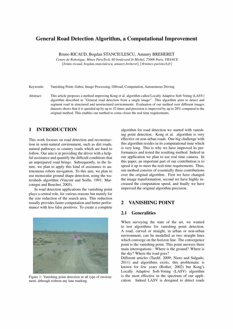
In road detection applications the vanishing pointplays a central role, for various reasons but mainly forthe size reduction of the search area. This reductionusually provides faster computation and better perfor-mance with less false positives. To create a complete

Figure 1: Vanishing point detection in all type of environ-ment, although without any lane marking.

algorithm for road detection we started with vanish-ing point detection. Kong et al. algorithm is veryeffective on non-urban roads. One big challenge withthis algorithm resides in its computational time whichis very long. This is why we have improved its per-formances and tested the resulting method. Indeed inour application we plan to use real time camera. Inthis paper, an important part of our contribution is tospeed it up to meet the real-time requirements. Thus,our method consists of essentially three contributionsover the original algorithm. First we have changedthe image transformation, second we have highly in-creased the computation speed, and finally we haveimproved the original algorithm precision.

2 VANISHING POINT

2.1 Generalities

When surveying the state of the art, we wantedto test algorithms for vanishing point detection.A road, curved or straight, in urban or non-urbanenvironment, can be modelled as two straight lineswhich converge on the horizon line. The convergencepoint is the vanishing point. This point answers threemain interrogations : Where is the ground? Where isthe sky? Where the road goes?Different articles (Tardif, 2009; Nieto and Salgado,2011) and algorithms exists, this problematic isknown for few years (Rother, 2002) but Kong’sLocally Adaptive Soft-Voting (LASV) algorithmis the most effective in the spectrum of our appli-cation. Indeed LASV is designed to detect roads

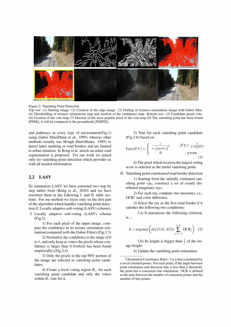
Figure 2: Vanishing Point Detection.Top row: (1) Starting image. (2) Creation of the edge image. (3) Finding of textures orientations image with Gabor filter.(4) Thresholding of textures orientations map and creation of the confidence map. Bottom row: (5) Candidate pixels vote.(6) Creation of the vote map (7) Election of the most popular pixel of the vote map (8) The vanishing point has been found[PINK], it will be compared to the groundtruth [WHITE].

and pathways in every type of environment(Fig.1)using Gabor filter(Dunn et al., 1995) whereas othermethods usually use Hough filter(Maitre, 1985) todetect lanes marking or road borders and are limitedto urban situation. In Kong et al. article an entire roadsegmentation is proposed. For our work we aimedonly for vanishing point detection which provides uswith all needed information.

2.2 LASV

To summarize LASV we have extracted two step bystep tables from (Kong et al., 2010) and we haverewritten them in the following I. and II. table sec-tions. For our method we focus only on the first partof the algorithm which handles vanishing point detec-tion (I. Locally adaptive soft-voting (LASV) scheme).I. Locally adaptive soft-voting (LASV) scheme

(Fig.2)1) For each pixel of the input image, com-

pute the confidence in its texture orientation esti-mation(computed with the Gabor Filter).(Fig.2.3)

2) Normalize the confidence to the range of 0to 1, and only keep as voters the pixels whose con-fidence is larger than 0.3(which has been foundempirically).(Fig.2.4)

3) Only the pixels in the top 90% portion ofthe image are selected as vanishing point candi-dates.

4) Create a local voting region Rv, for eachvanishing point candidate and only the voterswithin Rv vote for it.

5) Vote for each vanishing point candidate(Fig.2.6) based on :

Vote(P,V )=

{ 1

1+(

γd(P,V ))2 , if γ≥ 5

1+2d(P,V )

0 , γ even(1)

6) The pixel which receives the largest votingscore is selected as the initial vanishing point.

II. Vanishing point constrained road border detection1) Starting from the initially estimated van-

ishing point vp0, construct a set of evenly dis-tributed imaginary rays.

2) For each ray, compute two measures, i.e.,OCR1 and color difference.

3) Select the ray as the first road border if itsatisfies the following two conditions:

3.a) It maximizes the following criterion,ie., :

b = argimax(

di f f (A1,A2)xi+1

∑j=i−1

OCR j

)(2)

3.b) Its length is bigger than 13 of the im-

age height.4) Update the vanishing point estimation:

1Orientation Constitency Ratio : l is a line constituted bya set of oriented points. For each point, if the angle betweenpoint orientation and direction line is less than a threshold,the point has a consistent line orientation. OCR is definedas the ratio between the number of consistent points and thenumber of line points.

4.a) Regularly sample some points (with afour-pixel step) on the first road border denotedps.

4.b) Through each point of ps, respec-tively construct a set of 29 evenly distributed rays(spaced by 5◦, whose orientation from the hori-zon is more than 20◦, and less than 180◦) for eachpoint of ps, denoted as Ls

4.c) From each Ls, find a subset of n rayssuch that their OCRs rank top n among the 29rays.

4.d) The new vanishing point vp1 is se-lected from ps as the one which maximizes thesum of the top n OCRs1.

5) Starting from vp1, detect the second roadborder in a similar way as the first border, with aconstraint that the angle between the road bordersis larger than 20◦.

3 Our approach

Our interest in LASV (Kong et al., 2010)is motivated by the possibility of using it as apre-segmentation for our application. Our implemen-tation aims to work on a vehicle platform equippedwith a 30 FPS camera. This is why we needed toaccelerate its computation to meet the real timerequirements.We tested this algorithm on several datasets (Geigeret al., 2012; Kong et al., 2010; Leskovec et al.,2008), in our case this algorithm will be used withcontinuous capture. This is why we have tried toimprove this method on datasets using successiveframes instead of random environment picturesdatasets like the ones used by Kong.The original code was written in MATLAB by Kong.During the initial tests, the original implementationrequired a computation time of 18 seconds per image.Our optimisation is mainly concentrated on stepI.3) of the original algorithm. Our improvementswere done in the same environment in several steps.We have benchmarked each evolution to justify itspurpose.

3.1 Methods

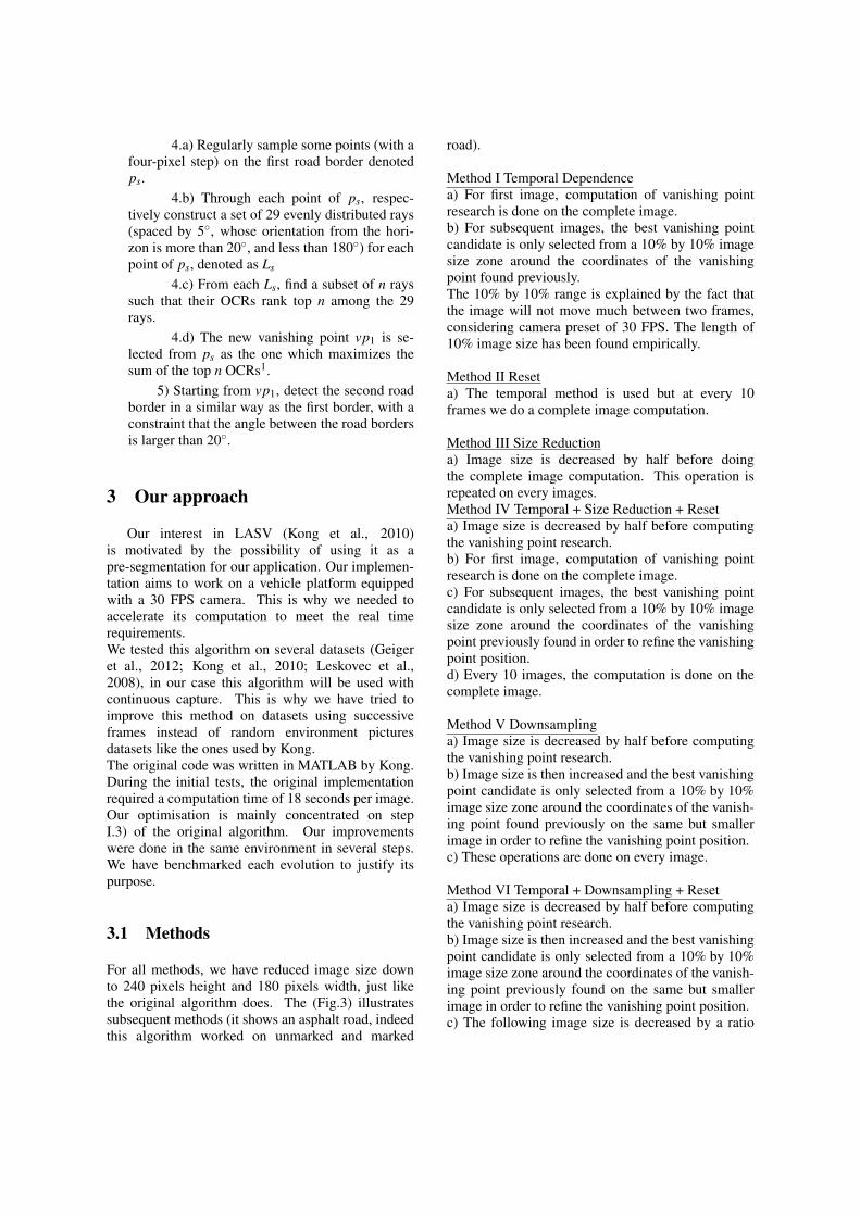
For all methods, we have reduced image size downto 240 pixels height and 180 pixels width, just likethe original algorithm does. The (Fig.3) illustratessubsequent methods (it shows an asphalt road, indeedthis algorithm worked on unmarked and marked

road).

Method I Temporal Dependencea) For first image, computation of vanishing pointresearch is done on the complete image.b) For subsequent images, the best vanishing pointcandidate is only selected from a 10% by 10% imagesize zone around the coordinates of the vanishingpoint found previously.The 10% by 10% range is explained by the fact thatthe image will not move much between two frames,considering camera preset of 30 FPS. The length of10% image size has been found empirically.

Method II Reseta) The temporal method is used but at every 10frames we do a complete image computation.

Method III Size Reductiona) Image size is decreased by half before doingthe complete image computation. This operation isrepeated on every images.Method IV Temporal + Size Reduction + Reseta) Image size is decreased by half before computingthe vanishing point research.b) For first image, computation of vanishing pointresearch is done on the complete image.c) For subsequent images, the best vanishing pointcandidate is only selected from a 10% by 10% imagesize zone around the coordinates of the vanishingpoint previously found in order to refine the vanishingpoint position.d) Every 10 images, the computation is done on thecomplete image.

Method V Downsamplinga) Image size is decreased by half before computingthe vanishing point research.b) Image size is then increased and the best vanishingpoint candidate is only selected from a 10% by 10%image size zone around the coordinates of the vanish-ing point found previously on the same but smallerimage in order to refine the vanishing point position.c) These operations are done on every image.

Method VI Temporal + Downsampling + Reseta) Image size is decreased by half before computingthe vanishing point research.b) Image size is then increased and the best vanishingpoint candidate is only selected from a 10% by 10%image size zone around the coordinates of the vanish-ing point previously found on the same but smallerimage in order to refine the vanishing point position.c) The following image size is decreased by a ratio

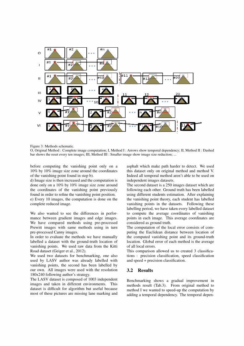
Figure 3: Methods schematic.O, Original Method : Complete image computation; I, Method I : Arrows show temporal dependency; II, Method II : Dashedbar shows the reset every ten images; III, Method III : Smaller image show image size reduction; ...

before computing the vanishing point only on a10% by 10% image size zone around the coordinatesof the vanishing point found in step b).d) Image size is then increased and the computation isdone only on a 10% by 10% image size zone aroundthe coordinates of the vanishing point previouslyfound in order to refine the vanishing point position.e) Every 10 images, the computation is done on thecomplete reduced image.

We also wanted to see the differences in perfor-mance between gradient images and edge images.We have compared methods using pre-processedPrewitt images with same methods using in turnpre-processed Canny images.In order to evaluate the methods we have manuallylabelled a dataset with the ground-truth location ofvanishing points. We used raw data from the KittiRoad dataset (Geiger et al., 2012).We used two datasets for benchmarking, one alsoused by LASV author was already labelled withvanishing points, the second has been labelled byour own. All images were used with the resolution180x240 following author’s strategy.The LASV dataset is composed of 1003 independentimages and taken in different environments. Thisdataset is difficult for algorithm but useful becausemost of these pictures are missing lane marking and

asphalt which make path harder to detect. We usedthis dataset only on original method and method V.Indeed all temporal method aren’t able to be used onindependent images datasets.The second dataset is a 250 images dataset which arefollowing each other. Ground truth has been labelledusing different students estimation. After explainingthe vanishing point theory, each student has labelledvanishing points in the datasets. Following theselabelling period, we have taken every labelled datasetto compute the average coordinates of vanishingpoints in each image. This average coordinates areconsidered as ground truth.The computation of the local error consists of com-puting the Euclidean distance between location ofthe computed vanishing point and its ground-truthlocation. Global error of each method is the averageof all local errors.This comparison allowed us to created 3 classifica-tions : precision classification, speed classificationand speed + precision classification.

3.2 Results

Benchmarking shows a gradual improvement inmethods result (Tab.3). From original method tomethod I we wanted to speed-up the computation byadding a temporal dependency. The temporal depen-

Method Speed (FPS)Method IV (gradient) 1.96Method IV (edge) 1.66Method VI (gradient) 0.71Method VI (edge) 0.66Method III (gradient) 0.53Method I 0.42Method V (gradient) 0.367Method III (edge) 0.366Method V (edge) 0.27Method II 0.21Original 0.06

Table 1: Speed Classification

Method PrecisionMethod V (gradient) 94.92%Original 93.50%Method III (gradient) 92.66%Method IV (gradient) 91.12%Method V (edge) 90.28%Method III (edge) 90.22%Method IV (edge) 84.80%Method VI (gradient) 83.26%Method VI (edge) 79.74%Method II 78.06%Method I 30.41%

Table 2: Precision Classification. Error is the average Eu-clidian distance between groundtruth and found vanishingpoint on all the dataset. Precision is this error compared tohalf the image size

dency provided a small speed-up (Tab.1) but also abig loss in precision (Tab.2). A precision of 65.2%on an image of 180x240 is extremely low, with tem-poral dependency, vanishing point detection is oftenlost. This explains method II which was created to de-crease the temporal dependency errors. We changeddependency to be used only on intervals (10 images).Indeed this method shows us that smaller steps givesmaller errors (Tab.2) but a longer computation time(Tab.1). The method III followed the original methodwhere images size is yet decreased. We wanted tosee to which point, images size reduction would evenbring enough information to be useful. This methodrevealed to be very effective in both speed and preci-sion (Tab.3).In method IV we used image reduction and tempo-ral dependency together which shows us very inter-esting results. Speed had been improved a lot but,a light loss was also present. This is why we havecontinued to search method which can bring speed-up and precision maintenance. In method V, we usedthe downsampling method, inspired by the FPDW

Method #Method IV (gradient) 1.786Method IV (edge) 1.41Method VI (gradient) 0.591Method VI (edge) 0.526Method III (gradient) 0,491Method V (gradient) 0,348Method III (edge) 0,33Method V (edge) 0,244Method II 0,164Method I 0,143Original 0,05

Table 3: Speed * Precision Classification

Method PrecisionOriginal 88.46%Method V (gradient) 88.01%

Table 4: Precision Classification on ENS Dataset (1003 im-ages in difficult situations. Error is the average Euclidiandistance between groundtruth and found vanishing point onall the dataset.

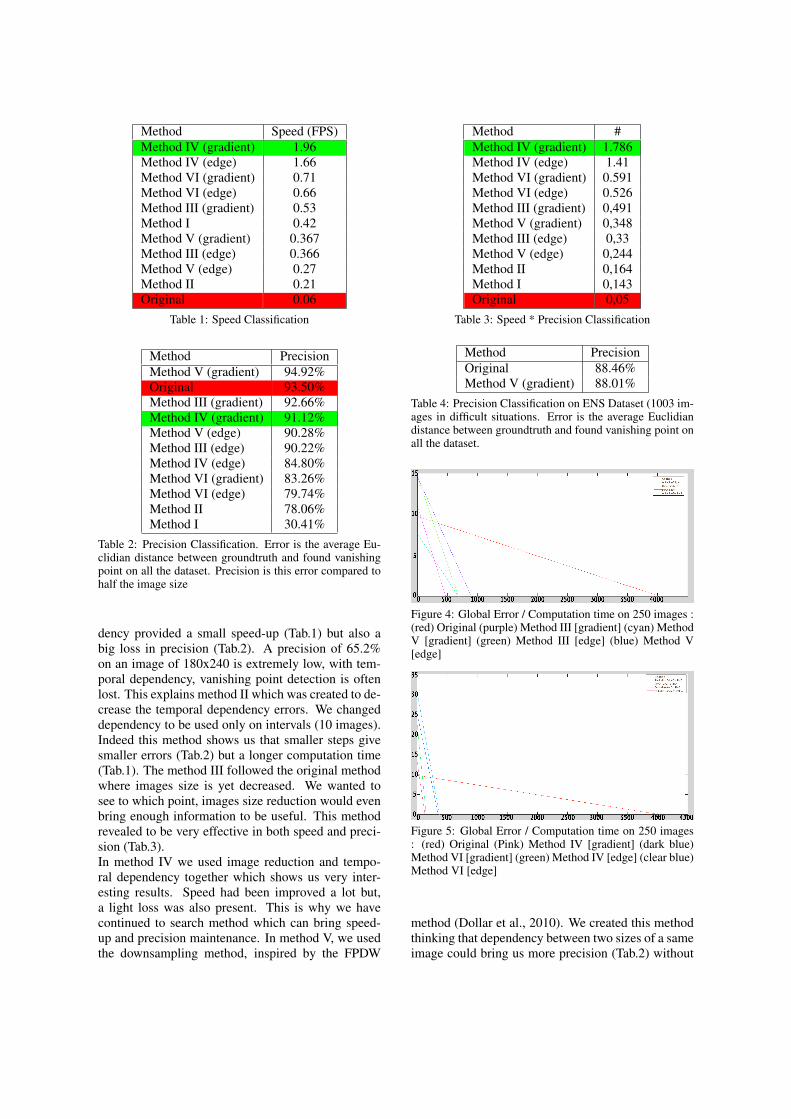
Figure 4: Global Error / Computation time on 250 images :(red) Original (purple) Method III [gradient] (cyan) MethodV [gradient] (green) Method III [edge] (blue) Method V[edge]

Figure 5: Global Error / Computation time on 250 images: (red) Original (Pink) Method IV [gradient] (dark blue)Method VI [gradient] (green) Method IV [edge] (clear blue)Method VI [edge]

method (Dollar et al., 2010). We created this methodthinking that dependency between two sizes of a sameimage could bring us more precision (Tab.2) without

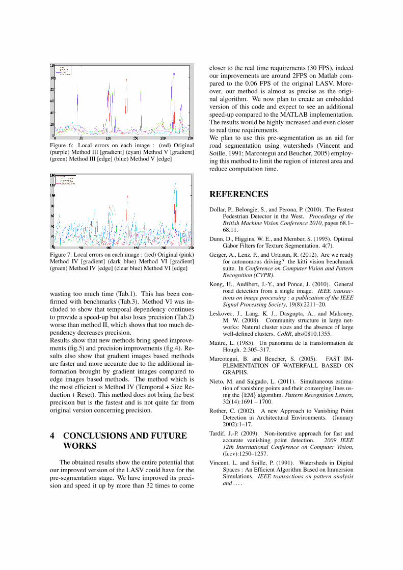
Figure 6: Local errors on each image : (red) Original(purple) Method III [gradient] (cyan) Method V [gradient](green) Method III [edge] (blue) Method V [edge]

Figure 7: Local errors on each image : (red) Original (pink)Method IV [gradient] (dark blue) Method VI [gradient](green) Method IV [edge] (clear blue) Method VI [edge]

wasting too much time (Tab.1). This has been con-firmed with benchmarks (Tab.3). Method VI was in-cluded to show that temporal dependency continuesto provide a speed-up but also loses precision (Tab.2)worse than method II, which shows that too much de-pendency decreases precision.Results show that new methods bring speed improve-ments (fig.5) and precision improvements (fig.4). Re-sults also show that gradient images based methodsare faster and more accurate due to the additional in-formation brought by gradient images compared toedge images based methods. The method which isthe most efficient is Method IV (Temporal + Size Re-duction + Reset). This method does not bring the bestprecision but is the fastest and is not quite far fromoriginal version concerning precision.

4 CONCLUSIONS AND FUTUREWORKS

The obtained results show the entire potential thatour improved version of the LASV could have for thepre-segmentation stage. We have improved its preci-sion and speed it up by more than 32 times to come

closer to the real time requirements (30 FPS), indeedour improvements are around 2FPS on Matlab com-pared to the 0.06 FPS of the original LASV. More-over, our method is almost as precise as the origi-nal algorithm. We now plan to create an embeddedversion of this code and expect to see an additionalspeed-up compared to the MATLAB implementation.The results would be highly increased and even closerto real time requirements.We plan to use this pre-segmentation as an aid forroad segmentation using watersheds (Vincent andSoille, 1991; Marcotegui and Beucher, 2005) employ-ing this method to limit the region of interest area andreduce computation time.

REFERENCES

Dollar, P., Belongie, S., and Perona, P. (2010). The FastestPedestrian Detector in the West. Procedings of theBritish Machine Vision Conference 2010, pages 68.1–68.11.

Dunn, D., Higgins, W. E., and Member, S. (1995). OptimalGabor Filters for Texture Segmentation. 4(7).

Geiger, A., Lenz, P., and Urtasun, R. (2012). Are we readyfor autonomous driving? the kitti vision benchmarksuite. In Conference on Computer Vision and PatternRecognition (CVPR).

Kong, H., Audibert, J.-Y., and Ponce, J. (2010). Generalroad detection from a single image. IEEE transac-tions on image processing : a publication of the IEEESignal Processing Society, 19(8):2211–20.

Leskovec, J., Lang, K. J., Dasgupta, A., and Mahoney,M. W. (2008). Community structure in large net-works: Natural cluster sizes and the absence of largewell-defined clusters. CoRR, abs/0810.1355.

Maitre, L. (1985). Un panorama de la transformation deHough. 2:305–317.

Marcotegui, B. and Beucher, S. (2005). FAST IM-PLEMENTATION OF WATERFALL BASED ONGRAPHS.

Nieto, M. and Salgado, L. (2011). Simultaneous estima-tion of vanishing points and their converging lines us-ing the {EM} algorithm. Pattern Recognition Letters,32(14):1691 – 1700.

Rother, C. (2002). A new Approach to Vanishing PointDetection in Architectural Environments. (January2002):1–17.

Tardif, J.-P. (2009). Non-iterative approach for fast andaccurate vanishing point detection. 2009 IEEE12th International Conference on Computer Vision,(Iccv):1250–1257.

Vincent, L. and Soille, P. (1991). Watersheds in DigitalSpaces : An Efficient Algorithm Based on ImmersionSimulations. IEEE transactions on pattern analysisand . . . .