BROYDEN’S AND THOMAS’ METHODS FOR IDENTIFYING
SINGULAR ROOTS IN NONLINER SYSTEMS
IKKA AFIQAH BINTI AMIR
A thesis submitted in partial fulfilment of the
requirement for the award of the degree of
Master of Science (Mathematic)
Faculty of Science
Universiti Teknologi Malaysia
JANUARY 2013

For my beloved mother and father,
Zaleha Maikon & Amir Hajib
My little sister and brothers,
My friends,
Raja Nadiah Raja Mohd Nazir
Nurfarhana Osman
Wan Khadijah Wan Sulaiman
and
Muhammad Nurhazrin Mohammad Nawi

ACKNOWLEDGEMENTS
First and foremost, thanks to Allah S.W.T, the Lord Almight for the health and
strength to complete this dissertation.
I would also like to express my most high gratitude to my supervisor, Tuan Haji
Ismail Bin Kamis for his comment and valuable advices. Thanks also to my examiner, P.M Dr
Rohanin Bin Ahmad for her patience in guiding me to complete this dissertation.
Special thanks to my beloved parents for their relentless blessing and support for me in
my journey to continue my studies. Appreciation has to be reserved to my siblings and all my
friends for their understanding and encouragement that has propelled me to make this
dissertation possible and worthwhile. Last but not least, I would like to say thank you for all
the people that involved in making this dissertation succesful either directly or indirectly.
ABSTRACT
Nonlinear systems is one of the mathematical models that is commonly used in the
engineering and science fields and it is quite complicated to determine the root especially
when the problem is singular. This study is conducted in order to study the performance of
Broyden’s and Thomas’ method, which are parts of Quasi-Newton method in solving singular
nonlinear systems. By applying the algorithm of each methods, we conduct the calculation to
achieve the approximate solutions. MATLAB software is used to compute and present the
solutions. Some of useful test problems would describe the properties and usage of the
methods. Hence, both methods that have been considered in this study give well approximate
solution but Thomas’ method gives better results than Broyden’s method.

ABSTRAK
Sistem tak lelurus adalah salah satu model matematik yang biasa digunakan dalam
bidang kejuruteraan dan sains dan ia agak rumit untuk mencari penyelesaian lebih- lebih lagi
apabila singular berlaku. Kajian ini dijalankan untuk mengkaji prestasi Broyden dan kaedah
Thomas yang merupakan sebahagian daripada Kaedah Kuasi-Newton dalam menyelesaikan
sistem linear tunggal. Dengan menggunakan algoritma setiap kaedah, kita melakukan
pengiraan untuk mendapatkan penyelesaian yang hampir. Perisian MATLAB juga digunakan
untuk mengira dan membentangkan penyelesaian. Beberapa contoh masalah dapat
menggambarkan sifat dan penggunaan kaedah ini. Oleh itu, kedua-dua kaedah yang telah
dipertimbangkan dalam kajian ini memberikan penyelesaian tetapi kaedah Thomas
memberikan hasil yang lebih baik daripada kaedah Broyden.

TABLE OF CONTENTS
CHAPTER TITLE PAGE
TITLE PAGE i
DECLARATION ii
DEDICATION iii
ACKNOWLEDGEMENTS iv
ABSTRACT v
ABSTRAK vi
TABLE OF CONTENTS vii
LIST OF TABLES x
LIST OF FIGURES xii
LIST OF APPENDICES xiii
LIST OF SYMBOLS xiv
1 INTRODUCTION 1
1.1 Introduction 1
1.2 Background of the Study 3
1.3 Statement of the Problem 4
1.4 Objective of the Study 5
1.5 Scope of the Study 5
1.6 Significance of the Study 5
2 LITERATURE REVIEW 6
2.1 Introduction 6
2.2 Nonlinear Systems 6
2.3 Newton Method 8
2.4 Quasi Newton Method 11
2.4.1 Broyden’s Method 12
2.4.2 Thomas’ Method 15
3 RESEARCH METHODOLOGY 16
3.1 Introduction 16
3.2 Research Framework 17
3.3 The Initial Point 18
3.4 Stopping Criterion 19
3.4.1 Properties of Broyden’s Method for
Singular Problems 20
3.5 Broyden’s Method 20
3.5.1 Flow Chart of Broyden’s Algorithm 22
3.6 Thomas’ Method 23
3.6.1 Flow Chart of Thomas’ Algorithm 25

4 RESULTS AND DISCUSSIONS 26
4.1 Introduction 26
4.2 Results 26
4.2.1 Example 4.1 27
4.2.2 Example 4.2 41
4.2.3 Example 4.3 44
4.2.4 Example 4.4 53
4.2.5 Example 4.5 57
4.3 Discussions 60
4.3.1 Number of Iteration 60
4.3.2 Descent Direction 61
4.3.2.1 Broyden’s Method 62
4.3.2.2 Thomas’ Method 63
5 SUMMARY, CONCLUSION AND
RECOMMENDATION 65
5.1 Introduction 65
5.2 Summary 65
5.3 Conclusion 66

5.4 Recommendation 67
REFERENCES 69
APPENDIX A 72
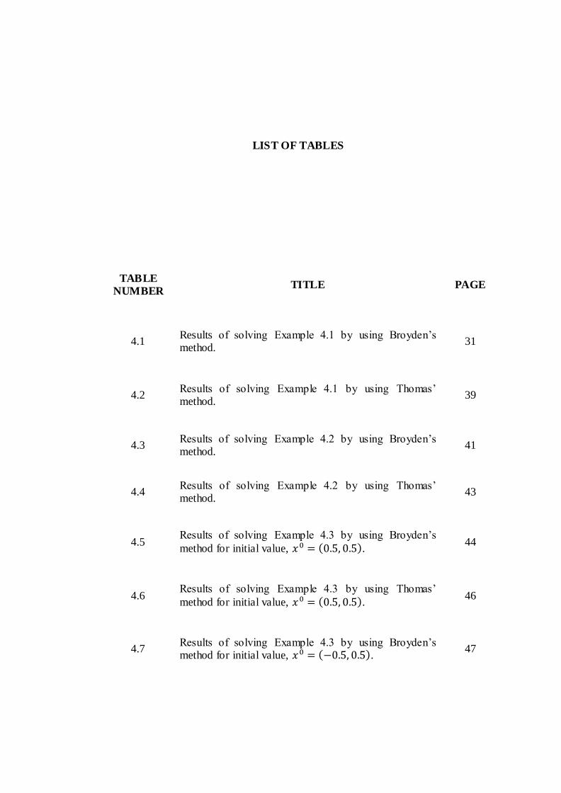
LIST OF TABLES
TABLE
NUMBER TITLE PAGE
4.1 Results of solving Example 4.1 by using Broyden’s method.
31
4.2 Results of solving Example 4.1 by using Thomas’ method.
39
4.3 Results of solving Example 4.2 by using Broyden’s method.
41
4.4 Results of solving Example 4.2 by using Thomas’ method.
43
4.5 Results of solving Example 4.3 by using Broyden’s
method for initial value, . 44
4.6 Results of solving Example 4.3 by using Thomas’
method for initial value, . 46
4.7 Results of solving Example 4.3 by using Broyden’s method for initial value, .
47

4.8 Results of solving Example 4.3 by using Thomas’ method for initial value, .
48
4.9 Results of solving Example 4.3 by using Broyden’s
method for initial value, . 50
4.10 Results of solving Example 4.3 by using Thomas’
method for initial value, . 51
4.11 Results of solving Example 4.4 by using Broyden’s
method for initial value, . 53
4.12 Results of solving Example 4.4 by using Thomas’ method for initial value, .
54
4.13 Results of solving Example 4.4 by using Broyden’s method for initial value, .
55
4.14 Results of solving Example 4.4 by using Thomas’ method for initial value, .
56
4.15 Results of solving Example 4.5 by using Broyden’s
method. 57
4.16 Results of solving Example 4.5 by using Thomas’ method.
58
4.17 The results of Broyden’s and Thomas’ method on
Example 4.1-4.5 60
4.18 The values of , for Example 4.3 by using Thomas’
method 63

4.19 Number of iteration in solving Example 4.3 by using
Thomas’ method 64
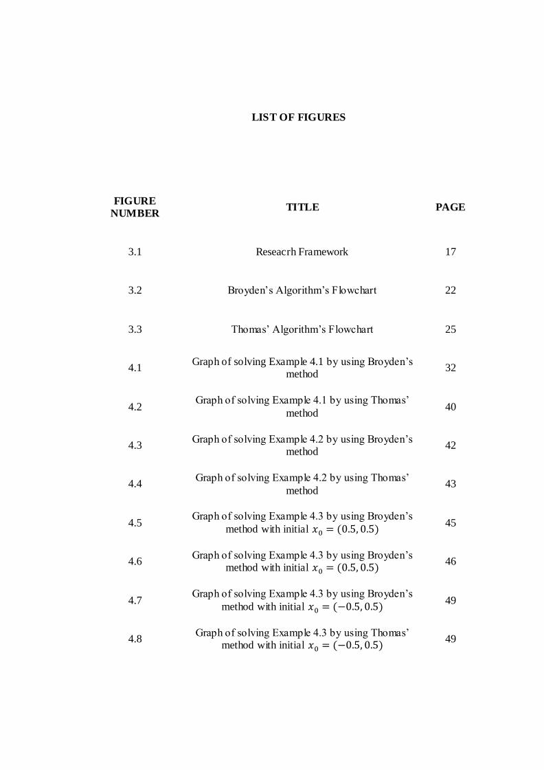
LIST OF FIGURES
FIGURE
NUMBER TITLE PAGE
3.1 Reseacrh Framework 17
3.2 Broyden’s Algorithm’s Flowchart 22
3.3 Thomas’ Algorithm’s Flowchart 25
4.1 Graph of solving Example 4.1 by using Broyden’s
method 32
4.2 Graph of solving Example 4.1 by using Thomas’
method 40
4.3 Graph of solving Example 4.2 by using Broyden’s
method 42
4.4 Graph of solving Example 4.2 by using Thomas’
method 43
4.5 Graph of solving Example 4.3 by using Broyden’s
method with initial 45
4.6 Graph of solving Example 4.3 by using Broyden’s
method with initial 46
4.7 Graph of solving Example 4.3 by using Broyden’s
method with initial 49
4.8 Graph of solving Example 4.3 by using Thomas’
method with initial 49

4.9 Graph of solving Example 4.3 by using Broyden’s
method with initial 52
4.10 Graph of solving Example 4.3 by using Thomas’
method with initial 52
4.11 Graph of solving Example 4.5 by using Broyden’s
method 59
4.12 Graph of solving Example 4.5 by using Thomas’
method 59

LIST OF APPENDICES
APPENDICE TITLE PAGE
A Coding MATLAB of Broyden’s and Thomas’ methods for solving singular nonlinear system
72

LIST OF SYMBOLS
- function of equation
- variable
- function of
- initial point
- local solution
- search direction in the iteration
- less than
- greater than
- equality
- less than or equal to
- greater than or equal to
- approximation
- limit value of norm
- epsilon, represents a very small
number, near zero
- infinity symbol
- Euler-Mascheroni constant.
- matrix of numbers
- absolute value
- norm
- matrix transpose
- inverse matrix

- rank of matrix A
- dimension of matrix A
ℝ - real numbers set
- limit value of a function
- the summation of
1
CHAPTER 1
INTRODUCTION
1.1 Introduction
Generally, linear systems can be described as the system that the output is
proportional to its input which is definitely contradic with a nonlinear systems. A
system is said to be nonlinear if it does not contain a linear system where it does not
satisfy the superposition principle and its output is not directly proportional to its
input. Nonlinear problem also arise in engineering, biology, physic and finance
field. In real world problem, most physical systems are inherently nonlinear, such as
Navier-Stokes equations in fluid dynamics, Lotka-Volterra in biology and Black-
Scholes Partial Differential Equation (PDE) in finance area. A nonlinear system
includes any problem that the variables need to be solved but cannot be presented as
a linear combination of independent components. Nonlinear equation is quite
complicated to solve. Infeasibility to combine the solutions to create new solutions is
one of the difficulties in solving nonlinear problems.

2
Nonlinear equations can be written as where is
nonlinear mapping. Consider there exists a solution . If is a singular
matrix then the nonlinear equations is singular and is a singular root at singular
point. Singular root or singular point is said to be the solution, though it is not unique
since there are many solution in the range that fulfill the condition of the equations.
To understand about singularity, Sánchez (1979) has shown the solution of second-
order equation that generally can be written as follows,
Based on the solution given, we can say it has singular point if and the
singular point can be classified as regular singular point if function and
in the equation have at most a pole of order 1 and 2 respectively at .
Since , therefore is a regular singular point of this equation, then the
solution is presented as
This is valid when , where represents any maximum value that
fulfill the condition of the solution. The expression showed that the solution cannot
be at single point as long as the singular points have no single value. The
points have any other value in the range between 0 and .
From previous discussion, the singular point obtained by the first derivative
of nonlinear equations, is a singular matrix where is a singular root. The
singularity of has potential to determine the convergence behavior of an
iterative sequence. Therefore, we consider that to be singular on the
and if it satisfied the singular assumptions
follows ( Buhmiler, 2010) :
3
i. is twice Lipschitz continuously differentiable.
ii. Rank .
iii. Let be the null space of spanned by and the
range space such that . For any projection
onto parallel to we assume
.
From this information, it is clear that when the problems have singularities,
we have difficulties to solve it. There are a lot of methods have been discussed that
possible to handle this problems.
1.2 Background of the Study
Dennis and Jorge (1977) have mentioned that nonlinear problems in finite
dimensions are generally solved by iteration and the known method for attacking this
problem is Newton’s method. Newton’s method fo r nonlinear equations can be
derived by assuming that we have an approximation to and that in a
neighbourhood of the linear mapping
is a good approximation to F. In this case, better approximation to can be
obtained by solving the linear system . Thus Newton’s method takes an
initial approximation to , and attempts to improve by the iteration,
(1.1)

4
If is invertible the Newton sequence (1.1) will converge quadratically
to if the initial guess, is sufficiently near . However, when fails to be
invertible we will say the point is singular. In this case, the Newton iterates will
not converge quadratically to . The convergence is to be linear if is chosen not
only near but in a special type of region that does not contain any ball about .
(Kelley and Suresh, 1983).
In addition, Dennis and Jorge (1977) have concluded that when Newton’s
methods is used to find a root and the derivative is singular at the root, convergence
of the Newton sequences is in general linear. They are also mentioned that the
disadvantages of Newton’s method are that a particular problem may require a very
good initial approximation to and need to determine for each k.
Hence, the Quasi-Newton method have been proposed as useful
modifications of Newton’s method for general nonlinear systems of equations.
Quasi-Newton methods have potential benefit in solving these algebraic system..
Because of the good potential of Quasi-Newton in solving nonlinear function, in this
study we will use Broyden’s and Thomas’ methods to get the solution for the
singular problems.
1.3 Statement of the Problem
This research will embark on a study of Broyden’s and Thomas’ methods,
ability in solving singular nonlinear systems.

5
1.4 Objectives of the Study
This study will be conducted to achieve the objectives as follows:
1.4.1 To code Broyden’s and Thomas’ algorithms using MATLAB.
1.4.2 To apply the Broyden’s and Thomas’ methods in solving singular
nonlinear systems.
1.4.3 To compare the performance of Broyden’s and Thomas’ algorithms.
1.4.4 To analyze the results of simulation and determine the efficiency of
both methods.
1.5 Scope of the Study
This study focuses on solving singular nonlinear systems. Broyden’s and
Thomas’ methods are used to handle this problem by approximation the Jacobian
according to the formula considered and then injected into the algorithm. The
algorithm for both methods is coded using MATLAB.
1.6 Significance of the Study
In solving singular nonlinear systems, it is hard to solve using the classical
method. Therefore, the Quasi-Newton methods are presented to solve the singular
nonlinear systems. This study will give us better understanding on the ability of
using the Quasi-Newton methods to solve singular problems. The Broyden’s and
Thomas’ methods are used due to their good behavior to approximate the Jacobian.

69
REFERENCES
Bertolazzi, E. (2005). Non-linear Problems in n Variables. Lectures for PHD course
on Non-linear Equations and Numerical Optimizationb. Universita di Trento
Biegler, L.T. (2000). Systems of Nonlinear Equations. Carnegie Mellon University
Pittsburgh: 1-27
Broyden, C. G. (1965). A Class of Methods for Solving Nonlinear Simultaneous
Equations.
Broyden, C. G. (1966). Quasi-Newton Methods and Their Application to Function
Minimisation. University College of Wales: 368-381
Brown, P. N., Hindmarsh, A. C., and Walker, H. F. (1985). Experiments with Quasi-
Newton Methods in Solving Stiff ODE Systems. Society for Industrial and
Applied Mathematics. 6(2): 297-313
Buhmiler, S., Krejic, N., and Lužanin, Z. (2010). Practical Quasi-Newton Algorithm
for Singular Nonlinear Systems. University of Novi Sad: 1-19.
Chen, X., Nashed, Z. and Qi, L. (1995). Convergence of Newton’s Method for
Singular Smooth and Nonsmooth Equations Using Adaptive Outer Inverse.
National Science Foundation Grant: 1-19
Chen, X. (1996). Superliner Convergence of Smoothing Quasi Newton Methods for
Nonsmooth Equations. Jounal of Computational and Applied Mathematics. 80:
105-126

70
Dennis, J.E. and Jorge, J. (1977). Quasi Newton Methods, Motivation and Theory.
Society for Industrial and Applied Mathematics. 19(1) pp 46-89
Kelley, C.T. and Suresh, R. (1983). A New Accelaration Method for Newton’s
Method at Singular Points. Society for Industrial and Applied Mathematics.
20(5) pp 1001-1009
Ojika, T. (1987). Modified Deflation Algorithm for the Solution of Singular
Problems. I. A systems of Nonlinear Algebraic Equations. Journal of
Mathematical Analysis and Application. 123(1): 199-221
Osinga, H.M. and Krauskopf, B. (2003). Fundamental of Algorithms Solving
Nonlinear Equations with Newton’s Method. University of Bristrol, UK: SIAM
publications. pp 85-95
Sánchez, D.A. (1979). Ordinary Differential Equations and Stability Theory: An
Introduction. University of New Mexico: Dover Publications,Inc.
Sun, D. and Han, J. (1997). Newton and Quasi Newton Methods for a Class of
Nonsmooth Equations and Related Problems. Society for Industrial and
Applied Mathematics. 7(2): 463-480
Schubert, L. K. (1969). Modification of a Quasi Newton Method for Nonlinear
Equations with a Sparse Jacobian. National Research Council of Canada and
Air Force Office of Scientific Research, United States Air Force: 27-35
Sun, L., He, G., Wang, Y., and Fang, L. (2009). An Active Set Quasi-Newton Method
with Project Search for Bound Constrained Minimization. Computer and
Mathematics with Applications. 58:161-170
Tapia, R. A. and Zhang, Y. (1992). On the Quadratic Convergence of the Singular
Newton’s Method. Ed. Larry Nasareth: pp 6-8, 1-6

71
Waziri, M. Y., Leong, W. J., and Hassan, M. A. (2011). Jacobian-Free Diagonal
Newton’s Method for Solving Nonlinear Systems with Singular Jacobian.
Malaysian Journal of Mathematical Sciences 5(2): 241-255
Recommended