Embed Size (px)
Citation preview
International Journal of Applied Science and Engineering 2013. 11, 1: 51-67
Int. J. Appl. Sci. Eng., 2013. 11, 1 51
A Numerical Patching Method for Solving Singular Perturbation Problems Via Padé Approximates
P. Padmajaa,* and Y. N. Reddyb
a Department of Mathematics, Prasad V Potluri Siddhartha Institute of Technology, Vijayawada, Andhra Pradesh, India
b Department of Mathematics, National Institute of Technology, Warangal, India Abstract: In this paper, we present a numerical patching method for solving a class of singularly perturbed two point boundary value problems with a boundary layer at one end point. In order to know the behavior of the solution of the singular perturbation problem in the boundary layer region, it is always suggestive to solve the problem in outer and boundary layer regions separately. By constructing a modified problem with a boundary layer correction, the boundary layer is dealt with separately and series method used. The condition at infinity will be applied to the corresponding Padé approximates of the obtained series solution. Several problems are solved to demonstrate the applicability and efficiency of the proposed method. It is observed that the present method approximates the exact solution very well. Keywords: Singular perturbation problems; boundary layer; boundary layer correction; Pade’
approximates.
* Corresponding author; e-mail: [email protected] Received 17 July 2012
Revised 24 September 2012 © 2013 Chaoyang University of Technology, ISSN 1727-2394 Accepted 1 October 2012
1. Introduction Singularly perturbed second order two-point boundary value problems arise very frequently in fluid mechanics and other branches of Applied Mathematics. These problems depend on a small positive parameter in such a way that the solution varies rapidly in some parts and varies slowly in some other parts. So, typically there are thin transition layers where the solutions can jump abruptly, while away from the layers the solution behaves regularly and vary slowly. The numerical treatment of the singular perturbation problems is far from the trivial because of the boundary layer behavior of the solution. There are a wide variety of methods for the solution of the singular perturbation problems. The notable methods are asymptotic expansion approximations. These methods consists of: (a) dividing the problem into an inner region (boundary layer) problem and an outer region problem; (b) expressing the inner and outer solutions as asymptotic expansions; (c) equating various terms in the inner and outer expressions to determine the constants in these expressions; and (d) combining the inner and outer solutions in some fashion to obtain a uniformly valid solution. Typically, the inner region problems are obtained from the original problem by rescaling the independent variable. These methods and their variations have been used successfully on a variety of linear and non-linear singular perturbation problems. However, there can be difficulties in applying these methods, such as the matching of the coefficients of the inner and outer expansions. Success may depend on finding the proper scaling or the proper transformation to express the dependent and independent

P. Padmaja and Y. N. Reddy
52 Int. J. Appl. Sci. Eng., 2013. 11, 1
variables. For a detailed theory and analytical discussion on singular perturbation problems one may refer to the books and high level monographs: O’ Malley [1], Nayfeh [2], Kevorkian and Cole [3], Bender and Orszag [4]. For a detailed Numerical and Asymptotic discussion on singular perturbation problems one may refer to the books and high level monographs: Hemker [5], Hemker and Miller [6], Miller [7-12], Miller et.al. [13], Axelson et.al. [14], Doolan et.al. [15], Holmes [16], Miranker [17], Morton [18], Aiken [19], Ardema [20], Goering et.al. [21] and Ross et.al. [22]. The survey paper by Kadalbajoo and Reddy [23], gives an erudite outline of the singular perturbation problems. Few other notable methods for solving singular perturbation problems are finite difference methods [24-26], finite element methods [27], boundary value technique [28-30], initial value techniques [31-33], spline techniques [34-35], and so on.
In order to know the behavior of the solution of the singular perturbation problem in the boundary layer region, it is always suggestive to solve the problem in outer and boundary layer regions separately. In this paper, we present a numerical patching method for solving a class of singularly perturbed two point boundary value problems with a boundary layer at one end point. By constructing a modified problem with a boundary layer correction, the boundary layer is dealt with separately and series method used. The condition at infinity will be applied to the corresponding Padé approximates of the obtained series solution. Several problems are solved to demonstrate the applicability and efficiency of the proposed method. It is observed that the present method approximates the exact solution very well. 2. A numerical patching method
For convenience we call our method the ‘a numerical patching method’. We consider a class of linear singular perturbed two point boundary value problem of the form
]1,0[x;)x(f)x(y)x(b)x(y)x(a)x(y (1)
with the conditions )0(y and )1(y (2)
where is a small positive parameter ( 10 ), and , are known constants. We assume that )x(fand)x(b,)x(a are sufficiently continuously differentiable functions in [0,1]. Furthermore, we assume that 0M)x(a , where M is some positive constant. This assumption merely implies that (1)-(2) has a solution which displays a boundary layer of width O() at 0x for small values of .
We obtain the reduced problem by setting =0 in equation (1) and solve it for the solution with the appropriate boundary condition. Let )x(U be the solution of the reduced problem of (1)-(2), i.e.;
)x(f)x(U)x(b)x(U)x(a with (3)
.)1(U (4)
It is well known from the singular perturbation theory that over most of the interval [0,1] the solution of (1)-(2) behaves like the solution of (3)-(4) but to satisfy the other boundary condition there is a small region in which the solution of (1)-(2) must deviate greatly from that of (3)-(4). This region is usually referred as boundary layer region. We choose so called stretching transformation ./xt

A Numerical Patching Method for Solving Singular Perturbation Problems Via Padé Approximates
Int. J. Appl. Sci. Eng., 2013. 11, 1 53
This transforms the equation (1) into
)t(fy)t(bdtdy)t(a
dtyd2
2 (5)
Upon setting 0 in (5), we have
0dtdy)0(a
dtyd2
2 (6)
If we require the solution to equation (5) to compensate for the fact that the solution of the reduce problem (3)-(4) does not satisfy the boundary condition at 0x , and further that this solution goes to zero as t , then we obtain the boundary layer correction problem
0t;0)t(V)0(a)t(V (7)
with 0)t(VLim,)0(U)0(Vt
(8)
Then, from standard singular perturbation theory it follows that the solution of (1) and (2) admits the representation in terms of the solutions of the reduced and boundary layer correction problems. Thus we can write the solution of (1)-(2) as an asymptotic expansion:
)(OxV)x(U)x(y
(9)
as 0 uniformly in ]1,0[ , with U the solution of (3)-(4) and V the solution of (7)- (8). The usual numerical methods can not be directly applied to (7)-(8) with out some modification. As will be seen, out boundary layer correction problem is one of such modification. The idea of
our method is to construct U and V in (9) such that the solution
xV)x(U)x(y can be used
to approximate the solution )x(y of (1)-(2). There is no perturbation parameter in (3)-(4), so it is easy to get the numerical solution by Runge-Kutta method. In fact any other standard analytical or numerical method can be used to solve the reduced problem (3)-(4). Although does not appear explicitly in the boundary layer correction problem (7)-(8), the semi infinite domain causes some difficulty. So we use the following technique: Let )0(V and we will determine the value of by using the condition 0)t(VLim
t
.
Thus (7) and (8) could be substituted by the initial problem,
0t;0)t(V)0(a)t(V (10)
with )0(V,)0(U)0(V (11)
The equation (10) is a constant coefficient linear differential equation and its solution is given by
)0(a))0(U(e
)0(a)t(V t)0(a
By using the condition 0)t(VLimt
, we get )0(U)0(a .
P. Padmaja and Y. N. Reddy
54 Int. J. Appl. Sci. Eng., 2013. 11, 1
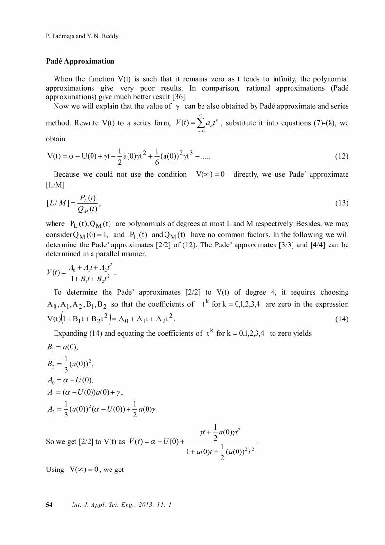
Padé Approximation
When the function V(t) is such that it remains zero as t tends to infinity, the polynomial approximations give very poor results. In comparison, rational approximations (Padé approximations) give much better result [36].
Now we will explain that the value of can be also obtained by Padé approximate and series
method. Rewrite V(t) to a series form,
0
)(n
nntatV , substitute it into equations (7)-(8), we
obtain
.....t))0(a(61t)0(a
21t)0(U)t(V 322 (12)
Because we could not use the condition 0)(V directly, we use Pade’ approximate [L/M]
,)()(]/[tQtPML
M
L (13)
where )t(Q),t(P ML are polynomials of degrees at most L and M respectively. Besides, we may consider ,1)0(QM and )t(PL and )t(QM have no common factors. In the following we will determine the Pade’ approximates [2/2] of (12). The Pade’ approximates [3/3] and [4/4] can be determined in a parallel manner.
.1
)( 221
2210
tBtBtAtAAtV
To determine the Pade’ approximates [2/2] to V(t) of degree 4, it requires choosing
21210 B,B,A,A,A so that the coefficients of 4,3,2,1,0kfor t k are zero in the expression
.tAtAAtBtB1)t(V 2210
221 (14)
Expanding (14) and equating the coefficients of 4,3,2,1,0kfor t k to zero yields
.)0(21))0(())0((
31
,)0())0((),0(
,))0((31
),0(
22
1
0
22
1
aUaA
aUAUA
aB
aB
So we get [2/2] to V(t) as .))0((
21)0(1
)0(21
)0()(22
2
tata
tatUtV
Using 0)(V , we get

A Numerical Patching Method for Solving Singular Perturbation Problems Via Padé Approximates
Int. J. Appl. Sci. Eng., 2013. 11, 1 55
.)0()0( Ua (15)
It is the same result as shown for the linear case. 2.1. Linear examples Example 1: Consider the following homogeneous singular perturbation problem
]1,0[x,0)x(y)x(y)x(y
with the boundary conditions 1)0( y and 1)1( y
The exact solution is given by
12
2112 11)( mm
mmmm
eeeeeexy
.
The reduced problem is 1)1(Uwith0)x(U)x(U
and its solution is .e)x(U 1x
The boundary layer correction problems is
)0(U)0(Vwith,0)t(V)t(V , )0(V .
Using the condition 0)(
tVLimt
we obtain 1e 1 .
Thus we obtain )1(1)1()( 11 teeetV , where
xt .
The required solution is .)1()( 11 x
x eeexy
The numerical results are given in Tables 1(a), 1(b) for =10-5 and 10-7 respectively.
Table 1. (a) 35 10,10 h ; (b) 37 10,10 h (a)
X y(x) Exact Solution (b) X y(x) Exact Solution
0.0000000 1.0000000 1.0000000 0.0020000 0.3686159 0.3681204 0.0040000 0.3693539 0.3688583 0.0060000 0.3700933 0.3695978 0.0080000 0.3708343 0.3703387 0.0100000 0.3715767 0.3710811 0.1000000 0.4065697 0.4060767 0.2000000 0.4493290 0.4488447 0.3000000 0.4965853 0.4961170 0.4000000 0.5488116 0.5483679 0.5000000 0.6065307 0.6061220 0.6000000 0.6703200 0.6699587 0.7000000 0.7408183 0.7405187 0.8000000 0.8187308 0.8185101 0.9000000 0.9048374 0.9047155 1.0000000 1.0000000 1.0000000
0.0000000 1.0000000 1.0000000 0.0020000 0.3686159 0.4097199 0.0040000 0.3693539 0.4104533 0.0060000 0.3700933 0.4111879 0.0080000 0.3708343 0.4119238 0.0100000 0.3715767 0.4126610 0.1000000 0.4065697 0.4472388 0.2000000 0.4493290 0.4890670 0.3000000 0.4965853 0.5348073 0.4000000 0.5488116 0.5848255 0.5000000 0.6065307 0.6395217 0.6000000 0.6703200 0.6993333 0.7000000 0.7408183 0.7647389 0.8000000 0.8187308 0.8362616 0.9000000 0.9048374 0.9144734 1.0000000 1.0000000 1.0000000

P. Padmaja and Y. N. Reddy
56 Int. J. Appl. Sci. Eng., 2013. 11, 1
Example 2: Consider the non homogeneous singular perturbation problem from fluid dynamics of small viscosity [37]
]1,0[,21)()( xxxyxy with the boundary conditions 0)0( y and 1)1( y .
The exact solution is given by
/1
/
1112)21()(
e
exxxyx
.
The reduced problem is 1)1(U,x21)x(U .
Its solution is .1)( 2 xxxU
The boundary layer correction problem is 1)0(Vwith,0)t(V)t(V and )0(V . Using the condition 0)t(VLim
t
we obtain 1 .
Hence .)( tetV
The required solution is .1)( 2 x
exxxy
The numerical results are given in Tables 2(a), 2(b) for =10-5 and 10-7 respectively.
Table 2. (a) 35 10,10 h ; (b) 37 10,10 h
(a) X y(x) Exact Solution
(b) X y(x) Exact Solution
0.0000000 0.0000000 0.0000000 0.0020000 -0.9979960 -0.9979760 0.0040000 -0.9959840 -0.9959641 0.0060000 -0.9939640 -0.9939441 0.0080000 -0.9919360 0.9919161 0.0100000 -0.9899000 -0.9898801 0.1000000 -0.8900000 -0.8899820 0.2000000 -0.7600000 -0.7599840 0.3000000 -0.6100000 -0.6099859 0.4000000 -0.4400000 -0.4399880 0.5000000 -0.2500000 -0.2499900 0.6000000 -0.0399999 -0.0399919 0.7000000 0.1900001 0.1900061 0.8000000 0.4400000 0.4400041 0.9000000 0.7100001 0.7100022 1.0000000 1.0000000 1.0000000
0.0000000 0.0000000 0.0000000 0.0020000 -0.9979960 -0.9979958 0.0040000 -0.9959840 -0.9959838 0.0060000 -0.9939640 -0.9939638 0.0080000 -0.9919360 -0.9919358 0.0100000 -0.9899000 -0.9898998 0.1000000 -0.8900000 -0.8899999 0.2000000 -0.7600000 -0.7599999 0.3000000 -0.6100000 -0.6099999 0.4000000 -0.4400000 -0.4399999 0.5000000 -0.2500000 -0.2499999 0.6000000 -0.0399999 -0.0399999 0.7000000 0.1900001 0.1900001 0.8000000 0.4400000 0.4400000 0.9000000 0.7100001 0.7100001 1.0000000 1.0000000 0.9999999
Example 3: Consider the variable coefficient singular perturbation problem [3]
]1,0[,0)(21)(
21)(
xxyxyxxy
with the boundary conditions 0)0( y and 1)1(y .

A Numerical Patching Method for Solving Singular Perturbation Problems Via Padé Approximates
Int. J. Appl. Sci. Eng., 2013. 11, 1 57
The exact solution is given by
4
2
21
21)(
xx
ex
xy .
The reduced problem is 1)1(,0)(21)(
21
UxUxUx
and
its solution is x
xU
2
1)( .
The boundary layer correction problem is
21)0(,0)()(
VwithtVtV and )0(V .
Using the condition 0)t(VLimt
we obtain 2/1 .
tetV 21)( .
The required solution is x
ex
xy
21
21)( .
The numerical results are given in Tables 3(a), 3(b) for =10-5 and 10-7 respectively.
Table 3. (a) 35 10,10 h ; (b) 37 10,10 h
(a) X y(x) Exact Solution
(b) X y(x) Exact Solution
0.0000000 0.0000000 0.0000000 0.0020000 0.5005005 0.5005005 0.0040000 0.5010020 0.5010020 0.0060000 0.5015045 0.5015045 0.0080000 0.5020080 0.5020080 0.0100000 0.5025126 0.5025126 0.1000000 0.5263158 0.5263158 0.2000000 0.5555556 0.5555556 0.3000000 0.5882353 0.5882353 0.4000000 0.6250000 0.6250000 0.5000000 0.6666667 0.6666667 0.6000000 0.7142857 0.7142857 0.7000000 0.7692308 0.7692308 0.8000000 0.8333333 0.8333333 0.9000000 0.9090909 0.9090909 1.0000000 1.0000000 1.0000000
0.0000000 0.0000000 0.0000000 0.0020000 0.5005005 0.5005005 0.0040000 0.5010020 0.5010020 0.0060000 0.5015045 0.5015045 0.0080000 0.5020080 0.5020080 0.0100000 0.5025126 0.5025126 0.1000000 0.5263158 0.5263158 0.2000000 0.5555556 0.5555556 0.3000000 0.5882353 0.5882353 0.4000000 0.6250000 0.6250000 0.5000000 0.6666667 0.6666667 0.6000000 0.7142857 0.7142857 0.7000000 0.7692308 0.7692308 0.8000000 0.8333333 0.8333333 0.9000000 0.9090909 0.9090909 1.0000000 1.0000000 1.0000000
2.2. Nonlinear singular perturbation problems
We consider a class of nonlinear singular perturbed two point boundary value problem of the form

P. Padmaja and Y. N. Reddy
58 Int. J. Appl. Sci. Eng., 2013. 11, 1
1x0;0)y,x(g)x(y)y,x(f)x(y (16)
with the boundary conditions
)0(y and )1(y (17)
where is a small positive parameter ( 10 ), and , are known constants. We assume that )y,x(f and )y,x(g are sufficiently continuously differentiable functions in
[0,1]. Furthermore, we assume that 0M)y,x(f , where M is some positive constant. This assumption merely implies that the boundary layer will be in the neighborhood of 0x .
The reduced problem is
0)U,x(g)x(U)U,x(f with )1(U (18)
Using the stretching transformation /xt equation (16) reduces to
.0)y,t(gdtdy)y,t(f
dtyd2
2 (19)
Setting 0 in (19) we have
.0dtdy)y,0(f
dtyd2
2 (20)
If we require the solution to (20) to compensate for the fact that the solution of the reduce problem (18) does not satisfy the boundary condition at 0x , and further that this solution goes to zero as t , then we obtain the boundary layer correction problem
0t;0)t(V)V)0(U,0(f)t(V (21)
with 0)(,)0()0(
tVLimUVt
(22)
Then, from standard singular perturbation theory it follows that the solution of (16) and (17) admits the representation in terms of the solutions of the reduced and boundary layer correction problems. Thus we can write the solution of (16)-(17) as an asymptotic expansion:
).(OxV)x(U)x(y
Although there is no in (18) and (21), it is difficult to apply the condition 0)t(VLimt
,
so we use the following technique in shooting method. Let )0(V and we will determine the value of by the condition 0)t(VLim
t
.
Thus equations (21) and (22) could be substituted by the initial problem,
0t;0)t(V)V)0(U,0(f)t(V (23)
with )0(,)0()0( VUV (24)
For nonlinear problems, we can not solve (23)-(24). Thus we use approximate method as (12)-(15). Form the numerical results it has been observed that the method is effective.

A Numerical Patching Method for Solving Singular Perturbation Problems Via Padé Approximates
Int. J. Appl. Sci. Eng., 2013. 11, 1 59
2.3. Nonlinear examples Example 4: Consider the nonlinear singular perturbation problem [2]
]1,0[x,0e)x(y2)x(y )x(y with the boundary conditions 1)1(and0)0( yy .
The exact solution is given by .)2(log1
2log)( /2 xee e
xxy
The reduced problem is .0)1(with02 UeU U
And its solution is .21
2ln)(
xxU
The boundary layer correction problems is
)2/1ln()0(,0)(2)( VwithtVtV and )0(V .
Using the condition 0)t(VLimt
we obtain
21log
21
.
.e)2/1ln()t(V t2
The required solution is .e21ln
21
2xln)x(y /x2
The numerical results are given in Tables 4(a), 4(b) for =10-3 and 10-4 respectively.
Table 4. (a) 35 10,10 h ; (b) 37 10,10 h
(a) X Y Exact Solution
(b) X Y Exact Solution
0.0000000 0.0000000 0.0000000 0.0020000 0.6911492 0.6911492 0.0040000 0.6891552 0.6891552 0.0060000 0.6871651 0.6871651 0.0080000 0.6851790 0.6851790 0.0100000 0.6831968 0.6831968 0.1000000 0.5978370 0.5978370 0.2000000 0.5108256 0.5108256 0.3000000 0.4307829 0.4307829 0.4000000 0.3566749 0.3566749 0.5000000 0.2876821 0.2876821 0.6000000 0.2231435 0.2231435 0.7000000 0.1625189 0.1625189 0.8000000 0.1053605 0.1053605 0.9000000 0.0512933 0.0512933 1.0000000 1.0000000 0.0000000
0.0000000 0.0000000 0.0000000 0.0020000 0.6911492 0.6911492 0.0040000 0.6891552 0.6891552 0.0060000 0.6871651 0.6871651 0.0080000 0.6851790 0.6851790 0.0100000 0.6831968 0.6831968 0.1000000 0.5978370 0.5978370 0.2000000 0.5108256 0.5108256 0.3000000 0.4307829 0.4307829 0.4000000 0.3566749 0.3566749 0.5000000 0.2876821 0.2876821 0.6000000 0.2231435 0.2231435 0.7000000 0.1625189 0.1625189 0.8000000 0.1053605 0.1053605 0.9000000 0.0512933 0.0512933 1.0000000 1.0000000 0.0000000

P. Padmaja and Y. N. Reddy
60 Int. J. Appl. Sci. Eng., 2013. 11, 1
Example 5: Consider the nonlinear singular perturbation problem [3] ]1,0[,0)()()()( xxyxyxyxy
with the boundary conditions 9995.3)1(and1)0( yy .
The exact solution is given by
2
tanh)(21
1
cxccxxy
where
11
log19995.21
1
121 c
cc
candc e .
The reduced problem is 9995.3)1(U,0UUU and its solution is .9995.2x)x(U The boundary layer correction problems is
9995.3)0(Vwith,0)t(V)V)0(U()t(V and .)0(V
We have to obtain using the condition .0)(
tVLimt
Taking the series
0n
nn ta)t(V and using it in boundary layer correction problem,
we get
.26347201,
611
61
32
201
)4(241,)(
61,
2,,9995.3
236
235
24
23210
aa
aaaaa
...........26347201
611
61
32
201)4(
241)(
61
29995.3)(
623
52342322
t
ttttttV
Using the Pade’ approximate [3/3]
33
221
33
2210
1)(
tBtBtBtAtAtAAtV
, we get
.02634720
1)(61)4(
241
611
61
32
201
06
1161
32
201
2)(
61)4(
241
0)4(241
2)(
61
)(61
29995.3
29995.3
9995.39995.3
233
22
21
23
2332
21
2
2321
2
21233
122
11
0
BBB
BBB
BBB
BBBA
BBA
BAA
A Numerical Patching Method for Solving Singular Perturbation Problems Via Padé Approximates
Int. J. Appl. Sci. Eng., 2013. 11, 1 61
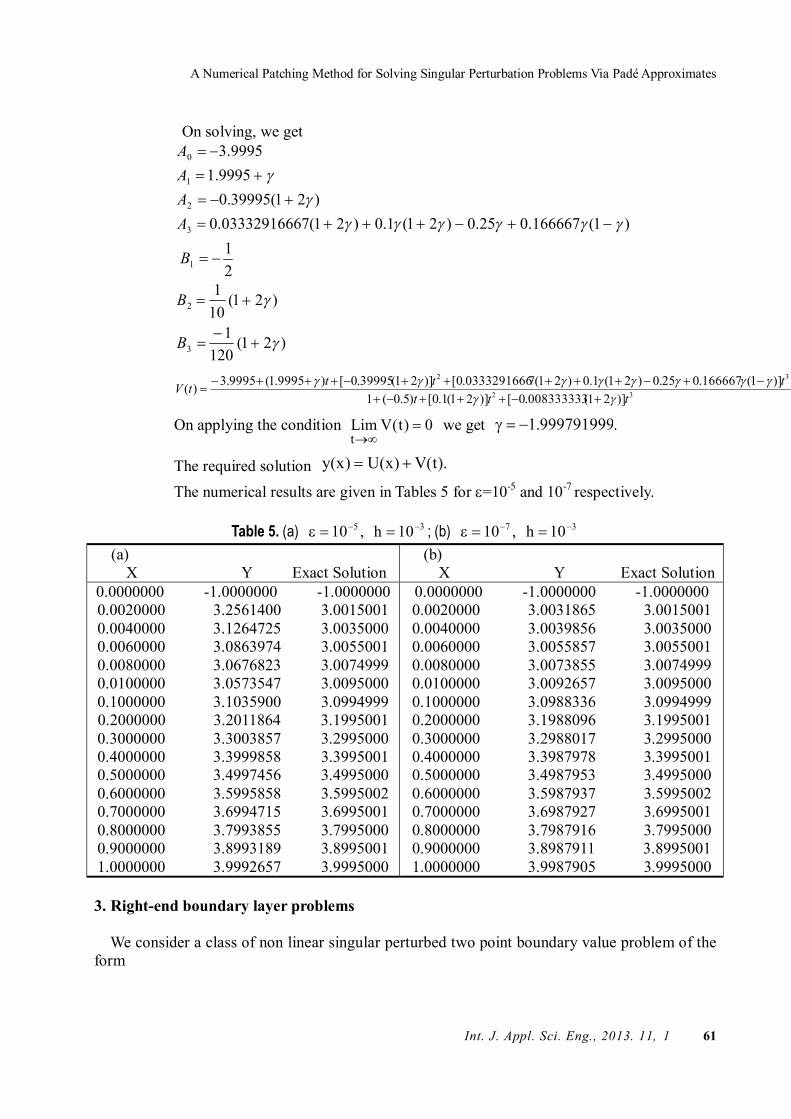
On solving, we get
21
)1(166667.025.0)21(1.0)21(70333291666.0)21(39995.0
9995.19995.3
1
3
2
1
0
B
AAAA
)21(120
1
)21(101
3
2
B
B
32
32
)]21(008333333.0[)]21(1.0[)5.0(1)]1(166667.025.0)21(1.0)21(70333291666.0[)]21(39995.0[)9995.1(9995.3)(
tttttttV
On applying the condition 0)t(VLimt
we get 999791999.1 .
The required solution ).t(V)x(U)x(y
The numerical results are given in Tables 5 for =10-5 and 10-7 respectively.
Table 5. (a) 35 10h ,10 ; (b) 37 10h ,10 (a)
X Y Exact Solution (b)
X Y Exact Solution 0.0000000 -1.0000000 -1.0000000 0.0020000 3.2561400 3.0015001 0.0040000 3.1264725 3.0035000 0.0060000 3.0863974 3.0055001 0.0080000 3.0676823 3.0074999 0.0100000 3.0573547 3.0095000 0.1000000 3.1035900 3.0994999 0.2000000 3.2011864 3.1995001 0.3000000 3.3003857 3.2995000 0.4000000 3.3999858 3.3995001 0.5000000 3.4997456 3.4995000 0.6000000 3.5995858 3.5995002 0.7000000 3.6994715 3.6995001 0.8000000 3.7993855 3.7995000 0.9000000 3.8993189 3.8995001 1.0000000 3.9992657 3.9995000
0.0000000 -1.0000000 -1.0000000 0.0020000 3.0031865 3.0015001 0.0040000 3.0039856 3.0035000 0.0060000 3.0055857 3.0055001 0.0080000 3.0073855 3.0074999 0.0100000 3.0092657 3.0095000 0.1000000 3.0988336 3.0994999 0.2000000 3.1988096 3.1995001 0.3000000 3.2988017 3.2995000 0.4000000 3.3987978 3.3995001 0.5000000 3.4987953 3.4995000 0.6000000 3.5987937 3.5995002 0.7000000 3.6987927 3.6995001 0.8000000 3.7987916 3.7995000 0.9000000 3.8987911 3.8995001 1.0000000 3.9987905 3.9995000
3. Right-end boundary layer problems
We consider a class of non linear singular perturbed two point boundary value problem of the form
P. Padmaja and Y. N. Reddy
62 Int. J. Appl. Sci. Eng., 2013. 11, 1
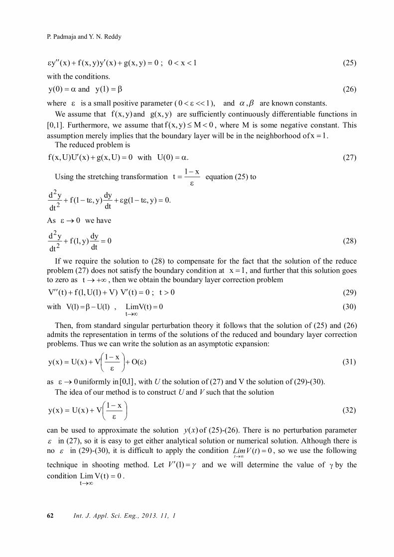
1x0;0)y,x(g)x(y)y,x(f)x(y (25)
with the conditions.
)0(y and )1(y (26)
where is a small positive parameter ( 10 ), and , are known constants. We assume that )y,x(f and )y,x(g are sufficiently continuously differentiable functions in
[0,1]. Furthermore, we assume that 0M)y,x(f , where M is some negative constant. This assumption merely implies that the boundary layer will be in the neighborhood of 1x .
The reduced problem is
0)U,x(g)x(U)U,x(f with .)0(U (27)
Using the stretching transformation
x1t equation (25) to
.0)y,t1(gdtdy)y,t1(f
dtyd2
2
As 0 we have
0dtdy)y,1(f
dtyd2
2 (28)
If we require the solution to (28) to compensate for the fact that the solution of the reduce problem (27) does not satisfy the boundary condition at 1x , and further that this solution goes to zero as t , then we obtain the boundary layer correction problem
0t;0)t(V)V)1(U,1(f)t(V (29)
with 0)t(VLim,)1(U)1(Vt
(30)
Then, from standard singular perturbation theory it follows that the solution of (25) and (26) admits the representation in terms of the solutions of the reduced and boundary layer correction problems. Thus we can write the solution as an asymptotic expansion:
)(Ox1V)x(U)x(y
(31)
as 0 uniformly in ]1,0[ , with U the solution of (27) and V the solution of (29)-(30). The idea of our method is to construct U and V such that the solution
x1V)x(U)x(y (32)
can be used to approximate the solution )(xy of (25)-(26). There is no perturbation parameter in (27), so it is easy to get either analytical solution or numerical solution. Although there is no in (29)-(30), it is difficult to apply the condition 0)(
tVLim
t, so we use the following
technique in shooting method. Let )1(V and we will determine the value of by the condition 0)t(VLim
t
.
A Numerical Patching Method for Solving Singular Perturbation Problems Via Padé Approximates
Int. J. Appl. Sci. Eng., 2013. 11, 1 63
Thus equations (29)-(30) could be substituted by the initial problem,
0t;0)t(V)V)1(U,1(f)t(V (33)
with .)1(V,)1(U)1(V (34)
Now we discuss the solution of (33)-(34). We use the series method. Let n
0nn )1t(a)t(V
,
and apply it into (33)-(34). We could get the value of ...),.........2,1,0( nan , and of course it is a expression corresponding to . Thus )t(V could be a series about and t . Using the condition 0)t(VLim
t
and rational approximate, we get the series solution of (33)-(34).
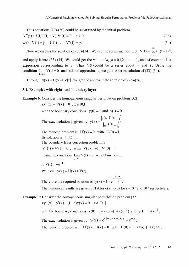
Through tV)x(U)x(y , we get the approximate solution of (25)-(26). 3.1. Examples with right -end boundary layer Example 6: Consider the homogeneous singular perturbation problem [32]
]1,0[x,0)x(y)x(y
with the boundary conditions .0)1(and1)0( yy
The exact solution is given by .
1e1e)x(y
/1
/)1x(
The reduced problem is 0)x(U with .1)0(U Its solution is .1)x(U The boundary layer correction problem is
.)0(V,1)0(Vwith,0)t(V)t(V
Using the condition 0)t(VLimt
we obtain .1
.e)t(V t
We have ).t(V)x(U)x(y
Therefore the required solution is .e1)x(y)-x1(
The numerical results are given in Tables 6(a), 6(b) for =10-5 and 10-7 respectively. Example 7: Consider the homogeneous singular perturbation problem [32]
]1,0[x,0)x(y)1()x(y)x(y
with the boundary conditions 11 e1)1(yand))1(exp(1)0(y .
The exact solution is given by x/)1x)(1( ee)x(y .
The reduced problem is 0)x(U)x(U with )/)1(exp(1)0(U .

P. Padmaja and Y. N. Reddy
64 Int. J. Appl. Sci. Eng., 2013. 11, 1
On solving we get .e)/)1(exp(1)x(U x
The boundary layer correction problem is, 0)t(V)t(V
with )/)21(exp(1)0(V and )0(V .
Using the condition 0)t(Vlimt
we obtain .1e /)21(
Hence .e)/)21(exp(1)t(V t
The required solution is
)-x1( x e )/)21(exp(1e)/)1(exp(1)x(y .
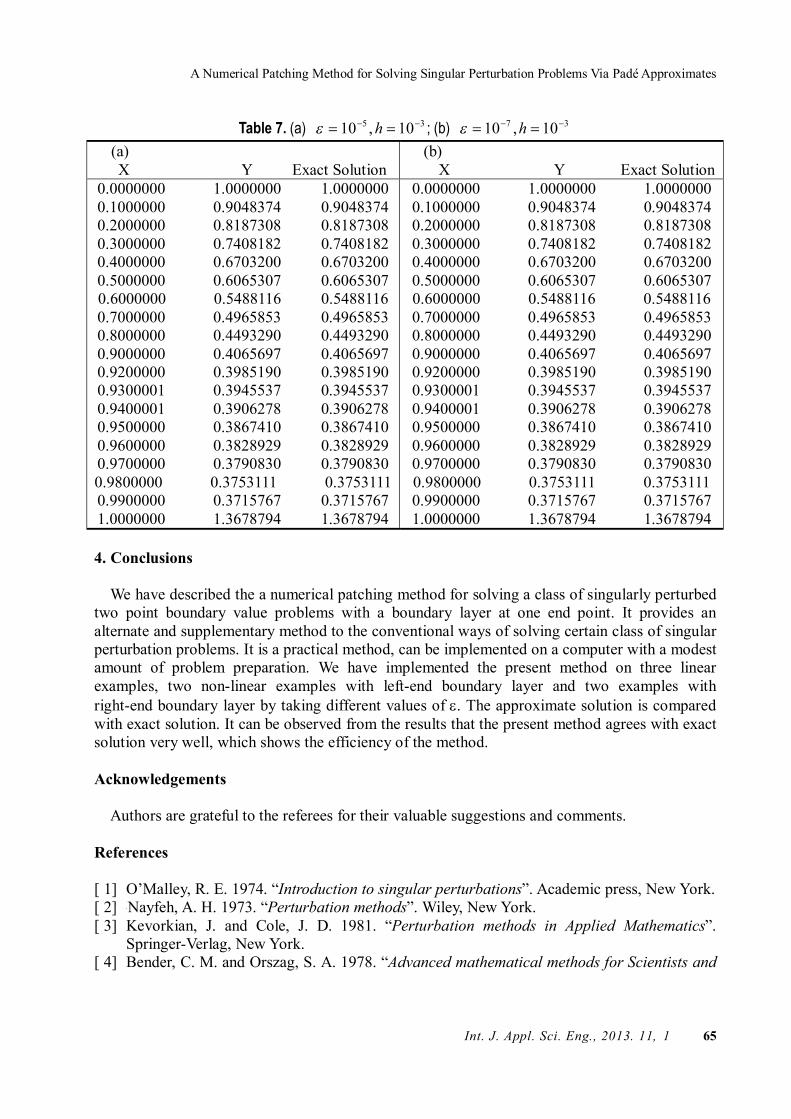
The numerical results are given in Tables 7(a), 7(b) for =10-5 and 10-7 respectively.
Table 6. (a) 35 10,10 h ; (b) 37 10,10 h (a)
X Y Exact Solution (b)
X Y Exact Solution 0.0000000 1.0000000 1.0000000 0.1000000 1.0000000 1.0000000 0.2000000 1.0000000 1.0000000 0.3000000 1.0000000 1.0000000 0.4000000 1.0000000 1.0000000 0.5000000 1.0000000 1.0000000 0.6000000 1.0000000 1.0000000 0.7000000 1.0000000 1.0000000 0.8000000 1.0000000 1.0000000 0.9000000 1.0000000 1.0000000 0.9200000 1.0000000 1.0000000 0.9300001 1.0000000 1.0000000 0.9400001 1.0000000 1.0000000 0.9500000 1.0000000 1.0000000 0.9600000 1.0000000 1.0000000 0.9700000 1.0000000 1.0000000 0.9800000 1.0000000 1.0000000 0.9900001 1.0000000 1.0000000 1.0000000 0.0000000 0.0000000
0.0000000 1.0000000 1.0000000 0.1000000 1.0000000 1.0000000 0.2000000 1.0000000 1.0000000 0.3000000 1.0000000 1.0000000 0.4000000 1.0000000 1.0000000 0.5000000 1.0000000 1.0000000 0.6000000 1.0000000 1.0000000 0.7000000 1.0000000 1.0000000 0.8000000 1.0000000 1.0000000 0.9000000 1.0000000 1.0000000 0.9200000 1.0000000 1.0000000 0.9300001 1.0000000 1.0000000 0.9400001 1.0000000 1.0000000 0.9500000 1.0000000 1.0000000 0.9600000 1.0000000 1.0000000 0.9700000 1.0000000 1.0000000 0.9800000 1.0000000 1.0000000 0.9900001 1.0000000 1.0000000 1.0000000 0.0000000 0.0000000
A Numerical Patching Method for Solving Singular Perturbation Problems Via Padé Approximates
Int. J. Appl. Sci. Eng., 2013. 11, 1 65
Table 7. (a) 35 10,10 h ; (b) 37 10,10 h (a) X Y Exact Solution
(b) X Y Exact Solution
0.0000000 1.0000000 1.0000000 0.1000000 0.9048374 0.9048374 0.2000000 0.8187308 0.8187308 0.3000000 0.7408182 0.7408182 0.4000000 0.6703200 0.6703200 0.5000000 0.6065307 0.6065307 0.6000000 0.5488116 0.5488116 0.7000000 0.4965853 0.4965853 0.8000000 0.4493290 0.4493290 0.9000000 0.4065697 0.4065697 0.9200000 0.3985190 0.3985190 0.9300001 0.3945537 0.3945537 0.9400001 0.3906278 0.3906278 0.9500000 0.3867410 0.3867410 0.9600000 0.3828929 0.3828929 0.9700000 0.3790830 0.3790830 0.9800000 0.3753111 0.3753111 0.9900000 0.3715767 0.3715767 1.0000000 1.3678794 1.3678794
0.0000000 1.0000000 1.0000000 0.1000000 0.9048374 0.9048374 0.2000000 0.8187308 0.8187308 0.3000000 0.7408182 0.7408182 0.4000000 0.6703200 0.6703200 0.5000000 0.6065307 0.6065307 0.6000000 0.5488116 0.5488116 0.7000000 0.4965853 0.4965853 0.8000000 0.4493290 0.4493290 0.9000000 0.4065697 0.4065697 0.9200000 0.3985190 0.3985190 0.9300001 0.3945537 0.3945537 0.9400001 0.3906278 0.3906278 0.9500000 0.3867410 0.3867410 0.9600000 0.3828929 0.3828929 0.9700000 0.3790830 0.3790830 0.9800000 0.3753111 0.3753111 0.9900000 0.3715767 0.3715767 1.0000000 1.3678794 1.3678794
4. Conclusions
We have described the a numerical patching method for solving a class of singularly perturbed two point boundary value problems with a boundary layer at one end point. It provides an alternate and supplementary method to the conventional ways of solving certain class of singular perturbation problems. It is a practical method, can be implemented on a computer with a modest amount of problem preparation. We have implemented the present method on three linear examples, two non-linear examples with left-end boundary layer and two examples with right-end boundary layer by taking different values of . The approximate solution is compared with exact solution. It can be observed from the results that the present method agrees with exact solution very well, which shows the efficiency of the method. Acknowledgements
Authors are grateful to the referees for their valuable suggestions and comments. References [ 1] O’Malley, R. E. 1974. “Introduction to singular perturbations”. Academic press, New York. [ 2]--Nayfeh, A. H. 1973. “Perturbation methods”. Wiley, New York. [ 3] Kevorkian, J. and Cole, J. D. 1981. “Perturbation methods in Applied Mathematics”.
Springer-Verlag, New York. [ 4] Bender, C. M. and Orszag, S. A. 1978. “Advanced mathematical methods for Scientists and

P. Padmaja and Y. N. Reddy
66 Int. J. Appl. Sci. Eng., 2013. 11, 1
Engineers”. Mc Graw-Hill, New York. [ 5] Hemker, P. W. 1977. “A numerical study of stiff two point boundary problems”. MCT 80,
Mathematical centre, Amsterdam. [ 6] Hemker, P. W. and Miller, J. J. H. (Eds.) 1979. “Numerical Analysis of singular
perturbation problems”. Academic Press, New York. [ 7] Miller, J. J. H. (Ed.) 1993. “Application of Advanced Computational Methods for Boundary
and Interior Layers”. Boole Press, Dublin. [ 8] Miller, J. J. H. (Ed.) 1980. “Boundary and Interior Layers: Computational and Asymptotic
methods (BAIL I) ”. Boole Press, Dublin. [ 9] Miller, J. J. H. (Ed.) 1984. “Boundary and Interior Layers: Computational and Asymptotic
methods, (BAIL III) ”. Boole Press, Dublin. [10] Miller, J. J. H. (Ed.) 1982. “Computational and Asymptotic Methods for Boundary and
Interior Layers, (BAIL II) ”. Boole Press, Dublin. [11] Miller, J. J. H. (Ed.) 1991. “Computational Methods for Boundary and Interior Layers in
several Dimensions”. Boole Press, Dublin. [12] Miller, J. J. H. 1975. A finite element method for a two-point boundary value problems with
a small parameter affecting the highest derivative, Banach Center Publications, 3, 143-146. [13] Miller, J. J. H., O’Riordan, E., and Shishkin, G. I. 1996. “Fitted Numerical methods for
singular perturbation problems”. World Scientific, River Edge, NJ. [14] Axelsson, O., Frank, L. S., and Van Der Sluis, A. ( Eds. ) 1981. “Analytical and Numerical
Approaches to Asymptotic Problems in Analysis”. North-Holland Publishers, Amsterdam. [15] Doolan, E. P., Miller, J. J. H., and Schilders, W. H. A. 1980. “Uniform Numerical Methods
for problems with Initial and Boundary Layers”. Boole Press, Dublin. [16] Holmes, M. H. 1995. “Introduction to perturbation methods”. Springer Verlag, Berlin. [17] Miranker, W. L. 1981. “Numerical Methods for Stiff Equations and Singular Perturbation
Problems”. Reidel, Dordrecht. [18] Morton, K. W. 1995. “Numerical solution of convection - diffusion problems”. Oxford
University press. [19]-Aiken, R. C. (Ed.) 1985. “Stiff Computation, Oxford University Press”. Oxford, England. [20] Ardema, M. D. (Ed.) 1983. “Singular Perturbations in systems and control”. Springer
Verlag, New York. [21] Goering, H., Felgenhauer, A., Lube, G., Roos, H.G., and Tobiska, L. 1983. “Singularly
Perturbed differential equations”. Akademic-Verlag, Berlin. [22] Roos, G., Stynes, M., and Tobiska, L. 1996. “Numerical methods for singularly perturbed
differential equations”. Springer Verlag, Berlin. [23] Kadalbajoo, M. K. and Reddy, Y. N. 1989. Asymptotic and numerical analysis of singular
perturbations; A Survey , Applied Mathematics and computation, 30: 223-259. [24] Chawla, M. M. 1978. A fourth order tridiagonal finite difference method for general
nonlinear two point boundary value problems with mixed boundary conditions, Journal of Institute of Mathematics and its applications, 21: 83-93.
[25] Su, Y. C. and Wu, Q. G. 1991. “An introduction to numerical methods for the singular perturbation problems (in Chinese) ”. Chongquing publishing house, Chongqing.
[26] Andargie, A. and Reddy, Y. N. 2007. Fitted fourth order tridiagonal finite difference method for singular perturbation problems, Applied mathematics and computation, 192, 90-1000.
[27] Stynes, M. and O’Riordan, E. 1986. A uniformly accurate finite element method for singular pertuebation problem in conservative form, SIAM journal of numerical analysis, 23: 369-375.

A Numerical Patching Method for Solving Singular Perturbation Problems Via Padé Approximates
Int. J. Appl. Sci. Eng., 2013. 11, 1 67
[28] Kadalbajoo, M. K. and Reddy, Y. N. 1988. A boundary value method for a class of non linear singular perturbation problems, Communications in Applied Numerical methods, 4: 587-594.
[29] Vigo-Aguiar, J. and Natesan, S. 2004. A parallel boundary value technique for singularly perturbed two point boundary value problems, The Journal of super computing, 27: 195-206.
[30] Lei Wang. 2004. A novel method for a class of nonlinear singular perturbation problems, Applied Mathematics and computation, 156: 847-856.
[31] Kadalbajoo, M. K. and Reddy, Y. N. 1987. Initial value technique for a class of non-linear singular perturbation problems, Journal of Optimization Theory and Applications, 53: 395-406.
[32] Reddy, Y. N. and Chakravarthy, P. P. 2004. An initial value approach for singularly perturbed two point boundary value problems, Applied mathematics and computation, 155: 95-110.
[33] Kadalbajoo, M. K. and Kumar, D. 2009. Initial value technique for singularly perturbed two point boundary value problemsusing an exponenetially fitted finite difference scheme, Computers and mathematics with applications, 57: 1147-1156.
[34] Aziz, T. and Khan, A. A. 2002. A spline method for second order singularly perturbed boundary value problems, Journal of computational and applied mathematics, 147: 445-452.
[35] Tirmizi, I. A., Fazal-i-Haq, and Siraj-ul-Islam. 2008. Non polynomial spline solution of singularly perturbed boundary value problems, Applied mathematics and computation, 196: 6-16.
[36] Jain, M. K., Iyengar, S. R. K., Jain, R. K. 1991. “Numerical methods for scientific and Engineering computation”. Wiley Eastern Limited, New Delhi.
[37] Reinhardt, H. J. 1980. Singular perturbation problems of difference methods for linear ordinary differential equations, Journal of applicable analysis, 10: 53-70.


![[For solving Cauchy singular integral equations]](https://img.pdfslide.us/doc/110x75/62ac1474e67c9e6dfe689f03/for-solving-cauchy-singular-integral-equations.jpg)