A NEUROLOGICAL MODEL FOR SHELL PATTERN FORMATION
by
Tyler Matthew WhiteAn Honors Thesis
Mathematical SciencesGeorge Mason University
Committee:
Evelyn Sander, Honors Thesis Director
Thomas Wanner
Timothy Sauer
Klaus G. Fischer, Chairman, Departmentof Mathematical Sciences
Date: Spring 2006George Mason UniversityFairfax, VA
A Neurological Model for Shell Pattern Formation
An honors thesis presented to the George Mason UniversityDepartment of Mathematical Sciences
By
Tyler Matthew WhiteAssociate of Science
Northern Virginia Community College, 2003
Director: Evelyn Sander, Associate ProfessorDepartment of Mathematical Sciences
Spring 2006George Mason University
Fairfax, VA

ii
Copyright c© 2006 by Tyler Matthew WhiteAll Rights Reserved

iii
Dedication
I dedicate this thesis to all my brothers and sisters in arms fighting around the world.
I have worked and trained beside many of you and all of you always remain in my
heart. I also know the toll it takes on all of your loved ones and I hope they stay
strong for you. I pray for peace and your safe return.

iv
Acknowledgments
Their are numerous persons I would like to thank. To begin with, I would like to
thanks my parents for raising me to be a strong individual and for showing me the
importance of education. They supported Karlys and myself while we pursued on
our undergraduate degrees. Without them, we would have never gotten to this point
in our lives. I would like to thank my younger brother Zachary for for giving me
someone to fight with as a younger child, and wish him the best of luck with his first
child which will be born in July. I would like to thank my wife, Karlys, for always
encouraging me and supporting me in every endeavor I have pursued. I would also
like to thank her for being brave enough to support me in my decision to leave the
military to pursue my education in Mathematics.
I would like to thank the United States Airforce for showing me what my life would
be like if I never strived to attain a higher position in life. I would like to thank my
seventh grade Life Science Teacher from Francis C. Hammond Jr. High School Mrs.
Bort. She was the first person to tell me I had potential ( what she actually said was,
”you have a good brain, why don’t you trying using it for a change?”). I would like to
think I took her advice. I would like to thank Mrs. Nancy Chovin of Antelope Valley
College who recognized my potential in mathematics and encouraged me to follow it.
I would like to thank all the wonderful Professor of Mathematics at George Mason
University not only for the great education they bestowed upon me, but for also being
very approachable and giving me great advice through the years. Specifically, I would
like to thank Dr. Evelyn Sander for being my adviser and holding my hand through
this process. Also, I would like to thank Dr. Sander, Dr. Goldin, and Dr. Wanner for

v
being such great teachers and believing in me enough to recommend me to graduate
school. Finally, I would like to thank Christine Amaya and Pat Hendrix for making
the Mathematics Department a welcome and comfortable place for all students.
I would also like to thank all the friends I have made over the years for their
support and encouragement. Specifically, I would like to thank Keith Fox, Catherine
Sausville, Samah Mahmoud, Sharif Thompson, Jason Youngblood, and Chris Vo for
being such close friends for the last few years. I would like to give a special thanks
to Robert Allen for encouraging me in writting my thesis and helping me edit it.
Finally, I would like to thank my committee members Dr. Sander, Dr. Sauer, and
Dr. Wanner for taking the time to help finish my thesis.

vi
Table of Contents
Page
Abstract . . . . . . . . . . . . . . . . . . . . . . . . . . . . . . . . . . . . . . . 0
1 Introduction . . . . . . . . . . . . . . . . . . . . . . . . . . . . . . . . . . 1
1.1 The Mollusc . . . . . . . . . . . . . . . . . . . . . . . . . . . . . . . . 1
1.2 The Model . . . . . . . . . . . . . . . . . . . . . . . . . . . . . . . . . 3
2 Numerical Methods . . . . . . . . . . . . . . . . . . . . . . . . . . . . . . 8
2.1 The Programs . . . . . . . . . . . . . . . . . . . . . . . . . . . . . . . 8
2.1.1 Homogeneous Equilibrium . . . . . . . . . . . . . . . . . . . . 8
2.1.2 Convolution . . . . . . . . . . . . . . . . . . . . . . . . . . . . 9
2.1.3 Pattern Generation Using C++ . . . . . . . . . . . . . . . . . 13
2.2 Analysis Using Maple . . . . . . . . . . . . . . . . . . . . . . . . . . . 14
2.3 Matlab . . . . . . . . . . . . . . . . . . . . . . . . . . . . . . . . . . . 15
3 Model Analysis . . . . . . . . . . . . . . . . . . . . . . . . . . . . . . . . . 16
3.1 Analysis of the Discrete Time Model . . . . . . . . . . . . . . . . . . 16
3.1.1 Linearization of the Discrete Time Model . . . . . . . . . . . . 16
3.1.2 Analysis of Linearized Model . . . . . . . . . . . . . . . . . . 19
3.2 +1 Bifurcation . . . . . . . . . . . . . . . . . . . . . . . . . . . . . . 24
3.2.1 Parameter Set 1 . . . . . . . . . . . . . . . . . . . . . . . . . . 25
3.2.2 Parameter Set 2 . . . . . . . . . . . . . . . . . . . . . . . . . . 29
3.2.3 Variation of Initial Conditions . . . . . . . . . . . . . . . . . . 31
3.3 −1 Bifurcation . . . . . . . . . . . . . . . . . . . . . . . . . . . . . . 32
3.3.1 Parameter Set 1 . . . . . . . . . . . . . . . . . . . . . . . . . . 32
3.3.2 Parameter Set 2 . . . . . . . . . . . . . . . . . . . . . . . . . . 34
3.3.3 Variation of Initial Conditions . . . . . . . . . . . . . . . . . . 37
3.4 Complex Bifurcation . . . . . . . . . . . . . . . . . . . . . . . . . . . 38
3.4.1 Parameter Set 1 . . . . . . . . . . . . . . . . . . . . . . . . . . 39
3.4.2 Parameter Set 2 . . . . . . . . . . . . . . . . . . . . . . . . . . 43
3.4.3 Variation of Initial Conditions . . . . . . . . . . . . . . . . . . 47
3.5 Multiple Bifurcations . . . . . . . . . . . . . . . . . . . . . . . . . . . 49

vii
3.5.1 Bifurcations thru Complex and -1 . . . . . . . . . . . . . . . . 49
3.5.2 Bifurcations thru +1 and -1 . . . . . . . . . . . . . . . . . . . 50
3.6 Analysis of the Rate of Divergence . . . . . . . . . . . . . . . . . . . 51
Bibliography . . . . . . . . . . . . . . . . . . . . . . . . . . . . . . . . . . . . . 53
A Source Code . . . . . . . . . . . . . . . . . . . . . . . . . . . . . . . . . . 54
A.1 C++ Code . . . . . . . . . . . . . . . . . . . . . . . . . . . . . . . . . 54
A.2 Maple Code . . . . . . . . . . . . . . . . . . . . . . . . . . . . . . . . 80
A.3 Matlab Code . . . . . . . . . . . . . . . . . . . . . . . . . . . . . . . 82
A.3.1 Nonlinear Pattern Grapher . . . . . . . . . . . . . . . . . . . . 82
A.3.2 Linear Pattern Grapher . . . . . . . . . . . . . . . . . . . . . 82

viii
List of Figures
Figure Page
1.1 Basic Gastropod Shell . . . . . . . . . . . . . . . . . . . . . . . . . . 2
1.2 Gastropod Anatomy[7] . . . . . . . . . . . . . . . . . . . . . . . . . . 3
1.3 The wj function for fixed qj and σj . . . . . . . . . . . . . . . . . . . 6
3.1 Bifurcation Triangle . . . . . . . . . . . . . . . . . . . . . . . . . . . 22
3.2 (a, b)-plane bifurcations for parameter set 1 and 2 . . . . . . . . . . . 26
3.3 Linear Pattern for a +1 Bifurcation of parameter set 1, Linear Pattern
at t = 40, 41 . . . . . . . . . . . . . . . . . . . . . . . . . . . . . . . 26
3.4 Eigenvalues for Parameter Set 1 . . . . . . . . . . . . . . . . . . . . . 27
3.5 Nonlinear Pattern for a +1 Bifurcation of parameter set 1, Nonlinear
Pattern at t = 750 . . . . . . . . . . . . . . . . . . . . . . . . . . . . 27
3.6 +1 Bifurcation Difference between Linear and Nonlinear . . . . . . . 28
3.7 Linear +1 Bifurcation for Parameter Set 2, Linear Pattern at t = 40, 41 29
3.8 Eigenvalues for Parameter Set 2 . . . . . . . . . . . . . . . . . . . . . 29
3.9 Nonlinear +1 Bifurcation for Parameter Set 2, Nonlinear Pattern at
t = 750 . . . . . . . . . . . . . . . . . . . . . . . . . . . . . . . . . . 30
3.10 +1 Bifurcation Difference between Linear and Nonlinear for Parameter
Set 2 . . . . . . . . . . . . . . . . . . . . . . . . . . . . . . . . . . . . 31
3.11 Nonlinear +1 Bifurcation of Parameter Set 1 with a Different Number
of Vertical Stripes . . . . . . . . . . . . . . . . . . . . . . . . . . . . 31
3.12 (a, b)-plane Bifurcations for Parameter Set 1 . . . . . . . . . . . . . . 33
3.13 The eigenvalues for Parameter Set 1 . . . . . . . . . . . . . . . . . . . 34
3.14 Linear -1 Bifurcation for Parameter Set 1 . . . . . . . . . . . . . . . . 34
3.15 Nonlinear -1 Bifurcation for Parameter Set 1 . . . . . . . . . . . . . . 35
3.16 Difference Between the Linear and Nonlinear Patterns for Parameter
Set 1 . . . . . . . . . . . . . . . . . . . . . . . . . . . . . . . . . . . . 35
3.17 (a, b)-plane Bifurcations for Parameter Set 2 . . . . . . . . . . . . . . 36

ix
3.18 The eigenvalues for Parameter Set 2 . . . . . . . . . . . . . . . . . . . 36
3.19 Linear -1 Bifurcation for Parameter Set 2, Linear pattern at t = 15, 16 37
3.20 Nonlinear -1 Bifurcation for Parameter Set 2, Nonlinear pattern at
t = 750, 751 . . . . . . . . . . . . . . . . . . . . . . . . . . . . . . . . 37
3.21 Difference Between the Linear and Nonlinear Pattern for Parameter
Set 2 . . . . . . . . . . . . . . . . . . . . . . . . . . . . . . . . . . . . 38
3.22 Linear -1 Bifurcation for Parameter Set 1 with a Different Pattern . . 38
3.23 (a, b)-plane Bifurcations for Parameter Set 1 . . . . . . . . . . . . . . 39
3.24 Eigenvalues for Parameter Set 1 . . . . . . . . . . . . . . . . . . . . . 40
3.25 The 2π/arg(λ) for Parameter Set 1 . . . . . . . . . . . . . . . . . . . 40
3.26 Periodicity of Parameter Set 1 . . . . . . . . . . . . . . . . . . . . . . 41
3.27 Linear Complex Bifurcation for Parameter Set 1, Linear Pattern at
t = 550, 551, 552 . . . . . . . . . . . . . . . . . . . . . . . . . . . . . . 41
3.28 Nonlinear Complex Bifurcation for Parameter Set 1, Nonlinear Pattern
at t = 900, 901, 902 . . . . . . . . . . . . . . . . . . . . . . . . . . . . 42
3.29 Difference Between the Linear and Nonlinear Patterns for Parameter
Set 1 . . . . . . . . . . . . . . . . . . . . . . . . . . . . . . . . . . . . 42
3.30 The “V” Shape for both the Nonlinear and Linear Models for Param-
eter Set 1 . . . . . . . . . . . . . . . . . . . . . . . . . . . . . . . . . 43
3.31 (a, b)-plane Bifurcation Diagram for Parameter Set 2 . . . . . . . . . 44
3.32 Eigenvalues for Parameter Set 2 . . . . . . . . . . . . . . . . . . . . . 44
3.33 The 2π/arg(λ) for Parameter Set 2 . . . . . . . . . . . . . . . . . . . 45
3.34 Periodicity of Parameter Set 2 . . . . . . . . . . . . . . . . . . . . . . 45
3.35 Nonlinear Complex Bifurcation of Parameter Set 2, Nonlinear Pattern
at t = 750, 751, 752, 753 . . . . . . . . . . . . . . . . . . . . . . . . . . 46
3.36 Difference Between Linear and Nonlinear Patterns for Parameter Set 2 46
3.37 Eigenvalues and 2π/arg(λ) for the Parameter Set in Table 3.4 . . . . 47
3.38 Initial Conditions which are Period 5 in Time. . . . . . . . . . . . . . 48
3.39 Initial Conditions which are Period 19 in Time. . . . . . . . . . . . . 48
3.40 Patterns generated for γ = .87 for a pattern which is period 5 in and
period 19 in time. . . . . . . . . . . . . . . . . . . . . . . . . . . . . . 49
3.41 Nonlinear Bifurcation thru Complex and -1 . . . . . . . . . . . . . . . 50
3.42 Nonlinear Bifurcation thru +1 and -1 . . . . . . . . . . . . . . . . . . 50

x
3.43 Complex Bifurcations for γ = .463 and γ = .7 . . . . . . . . . . . . . 51
3.44 Complex Bifurcation for γ = .8 and γ = .999 . . . . . . . . . . . . . . 52
3.45 How || · ||∞ of the Difference of the Linear and Nonlinear Model varies
with respect to γ . . . . . . . . . . . . . . . . . . . . . . . . . . . . . 52

xi
List of Tables
Table Page
2.1 Comparison of Direct Convolution to Fourier Transform Convolution 12
2.2 Error Comparison of Direct Convolution to Fourier Transform Convo-
lution . . . . . . . . . . . . . . . . . . . . . . . . . . . . . . . . . . . 13
3.1 Parameter Values for +1 Bifurcations . . . . . . . . . . . . . . . . . 25
3.2 Parameter Values for -1 Bifurcations . . . . . . . . . . . . . . . . . . 32
3.3 Parameter Values for Complex Bifurcations . . . . . . . . . . . . . . 38
3.4 Parameter Values for Complex Bifurcations with Period 5 and 19 . . 47
3.5 Parameter Values for Bifurcation which are both Complex and -1 . . 49
3.6 Parameter Values for Bifurcation which are both +1 and -1 . . . . . . 50
3.7 Parameter Values for Bifurcation which are both +1 and -1 . . . . . . 51

Abstract
A NEUROLOGICAL MODEL FOR SHELL PATTERN FORMATION
Tyler Matthew White
George Mason University, 2006
Honors Thesis Director: Evelyn Sander
The pattern formations of mollusk shells have been examined for millennia. We
consider a neurological model for the central ganglion control pigmentation in shell
pattern formation which is discrete in time and continuous in space. We will assume
that the pattern is governed by the central ganglion and the amount of pigmentation
to be secreted at a particular point in space and time is nonlocally coupled to all
points in space at the previous time. This model is nonlinear. Therefore previous
analyses are based on linearization and using eigenfunction expansions to approximate
solutions. In this project we are studying the degree of error that comes from using
these approximation techniques rather than the full nonlinear system. It is our hope
that the results of this analysis will lead us to be able to isolate why certain patterns
are selected over others.
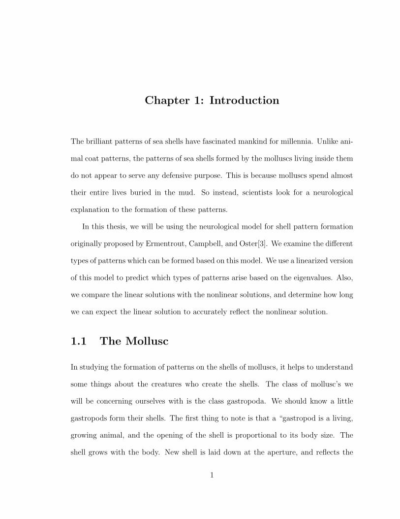
Chapter 1: Introduction
The brilliant patterns of sea shells have fascinated mankind for millennia. Unlike ani-
mal coat patterns, the patterns of sea shells formed by the molluscs living inside them
do not appear to serve any defensive purpose. This is because molluscs spend almost
their entire lives buried in the mud. So instead, scientists look for a neurological
explanation to the formation of these patterns.
In this thesis, we will be using the neurological model for shell pattern formation
originally proposed by Ermentrout, Campbell, and Oster[3]. We examine the different
types of patterns which can be formed based on this model. We use a linearized version
of this model to predict which types of patterns arise based on the eigenvalues. Also,
we compare the linear solutions with the nonlinear solutions, and determine how long
we can expect the linear solution to accurately reflect the nonlinear solution.
1.1 The Mollusc
In studying the formation of patterns on the shells of molluscs, it helps to understand
some things about the creatures who create the shells. The class of mollusc’s we
will be concerning ourselves with is the class gastropoda. We should know a little
gastropods form their shells. The first thing to note is that a “gastropod is a living,
growing animal, and the opening of the shell is proportional to its body size. The
shell grows with the body. New shell is laid down at the aperture, and reflects the
1

2
Figure 1.1: Basic Gastropod Shell[8]
size of the growing body”[7]. From Figure 1.1, we can see that the aperture of the
shell is the opening of the shell. The shell of a gastropod takes the form of a spiral,
so the growth of a shell starts from a central point and spirals outward. Now we will
talk about some of anatomical features of gastropods.
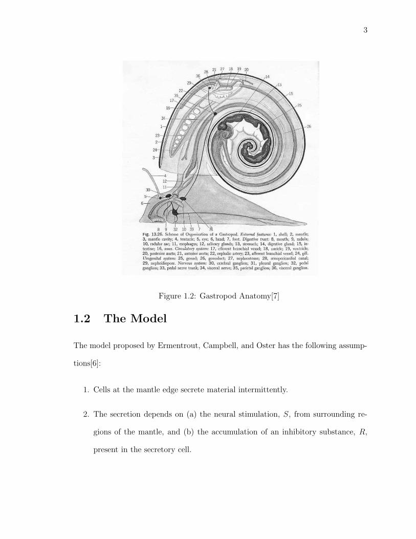
This thesis is concerned with a neurological model for shell pattern formation,
thus we should know a little about the nervous system of the gastropod. Figure 1.2
shows an image of the inner workings of a particular gastropod. In this model, we
will be concerned with the central ganglia of the mollusc. The central ganglion is not
listed in Figure 1.2, but we believe the central ganglion is just a combination of the
all the various ganglions, such as the cerebral ganglion. Also from Figure 1.2, we can
see the mantle of the shell. In the model we will be working with in this thesis, we
will assume that the shell is formed at the mantel edge. Now that we have a basic
understanding of gastropods, we can begin studying the model.
3
Figure 1.2: Gastropod Anatomy[7]
1.2 The Model
The model proposed by Ermentrout, Campbell, and Oster has the following assump-
tions[6]:
1. Cells at the mantle edge secrete material intermittently.
2. The secretion depends on (a) the neural stimulation, S, from surrounding re-
gions of the mantle, and (b) the accumulation of an inhibitory substance, R,
present in the secretory cell.

4
3. The net neural stimulation of the secretory cells consists of the difference be-
tween the excitatory and inhibitory inputs from the surrounding tissue.
From these assumptions, we need a functional S : R × C0(Ω) → R to determine
the neural stimulation of the surrounding regions of the mantle. By C0(Ω), mean the
set of all continuous functions from Ω to Ω. We will also need a function R(t, x) :
N∪0×R → R which gives the amount of inhibitory substance at time t and location
x. The model also tells us that the amount of pigmentation, P (t, x) : N∪0×R → R
laid down at a particular time t and space x is the difference in the neural stimulation
and inhibitory substance. Based on this definition, we get the following recurrence
relationship for P :
P (t + 1, x) = S(x, P (t, x)) − R(t, x). (1.1)
We will also assume that R “depends linearly on the amount of pigment secreted
during the previous period while at the same time degrading at a constant rate δ”[6].
The recurrence relationship for R is
R(t + 1, x) = γP (t, x) + δR(t, x), (1.2)
where 0 < γ < 1 is the rate of increase of pigmentation material, and 0 < δ < 1 is
the rate of decrease of inhibitory material.
Now we will define the neural stimulation functional S. Based on our assumptions,
S is dependent on the surrounding regions of the mantle. We will further assume
that the areas closer to the mantle will provide more stimulation than those which
are further away. Thus, we need a filtering function which we will call wj, j ∈ E, I
where wE is the excitatory filter, and wI is the inhibitory filter. We will define

5
wj : R → R in the following way:
wj(x) = 0 for |x| > σj, j ∈ E, I,
wj(x) = qj
2p −[
1 − cos
(
πx
σj
)]p
for |x| ≤ σj, j ∈ E, I.(1.3)
Equation (1.3) was defined this way in [3]. However, a truncated exponential function
would also work but would be discontinuous. The graph of this equation for a partic-
ular value of qj and σj can be seen in Figure 1.3. The parameter qj can be thought
of as a scaling factor that when multiplied to in integral in wj gives us αj as seen in
equation (1.4). The parameter p can be thought of as controlling the sharpness of
the cut-off.∫
Ω
wj(x)dx = αj, j ∈ E, I. (1.4)
Therefore, we choose qj based on the parameter value αj, which is the amplitude of
the excitatory and inhibitory kernel functions. Also, σj is the measure of the range
of the kernels. Using wj as our filter, we now must apply it to P . Let us define
E : R× C0(Ω) → C0(Ω) to be the convolution of f with wE,
E(x, f) =
∫
Ω
wE(|x′ − x|)f(x′)dx′ = (wE ∗ f)(x). (1.5)
Let us define I : R× C0(Ω) → C0(Ω)
I(x, f) =
∫
Ω
wI(|x′ − x|)f(x′)dx′ = (wI ∗ f)(x). (1.6)

6
2
5.6
4.0
0
2.4
−2x
8.0
3
7.2
6.4
4.8
1
3.2
1.6
−1
0.8
0.0
−3
Figure 1.3: The wj function for fixed qj and σj
Thus we are just performing a convolution on P and wj. Now we can define the
neural stimulation functional S : R× C0(Ω) → R as follows
S(x, f) = SE(E(x, f)) − SI(I(x, f)),
Sj : R → R,
Sj(u) = 1 + e−vj(u−θj)−1, j ∈ E, I.
(1.7)
We see that SE(E(x, f)) and SI(I(x, f)) are well defined for a fixed x. Clearly from
the definition, the function S is nonlinear, making the model itself nonlinear. Thus,
we will need to use linearization methods to perform analysis on the model. This will
be done later in Chapter 3.
We can reduce equations (1.1) and (1.2) into one recurrence relation. To do this,
we will begin by taking equation (1.1) and taking one step forward in time. So we

7
get,
P (t + 2, x) = S(x, P (t + 1, x)) − R(t + 1, x). (1.8)
Now take equation (1.2) and substitute it into equation (1.8). This give us,
P (t + 2, x) = S(x, P (t + 1, x)) − (γP (t, x) + δR(t, x)). (1.9)
Going back to equation (1.1), we can solve for R(t, x) which gives us R(t, x) =
S(x, P (t, x)) − P (t + 1, x). Take this value for R(t, x) and plug that into equation
(1.9) which gives us,
P (t + 2, x) = S(x, P (t + 1, x)) − (γP (t, x) + δ(S(x, P (t, x)) − P (t + 1, x))). (1.10)
Rearranging terms our recurrence relation becomes,
P (t + 2, x) = S(x, P (t + 1, x)) + δP (t + 1, x) − δS(x, P (t, x)) − γP (t, x). (1.11)
Equation (1.11) give us a recurrence relation for our model which does not depend
on R. From equation (1.11), we will generate our shell patterns. However, before we
begin this process, we must discuss the numerical techniques used to generate these
patterns and the accuracy of these methods.

Chapter 2: Numerical Methods
The numerical calculations performed in this thesis use a combination of custom
programs written in C++ , and the use of software packages such as Matlab and
Maple. The C++ programs are used to calculate the actual patterns using pre-built
libraries such as FFTW(Fastest Fourier Transform in the West). The Maple software
package was used to for stability analysis of the nonlinear system by using linear
approximations. Matlab was used to plot the patterns and aid in error analysis.
2.1 The Programs
A total of of three C++ programs were written for this thesis. The first program
calculated the nonlinear pattern, the second program calculated linearized pattern,
and final program made a comparison of the two patterns. Most of the programs are
very similar; their differences will be mentioned when they are relevant.
2.1.1 Homogeneous Equilibrium
For all the programs, we start by calculating a homogeneous equilibrium. First, a
definition of a homogeneous equilibrium.
Definition 2.1 (Homogeneous Equilibrium). An equilibrium is a point P (t, Ω) such
that
P (t1, Ω) = P (t2, Ω), ∀t1, t2 ∈ N ∪ 0,
8

9
so P (t, x) is unvarying with respect to t, so we can say that P (t, x) = P (x). A
homogeneous equilibrium is an equilibrium point P (x) such that
P (x) = P (y), ∀y ∈ Ω.
So P (t, x) is unvarying with respect to t and x, so we can say that P (t, x) = P0 for
some constant P0 ∈ Ω.
Computing the Homogeneous Equilibrium
To compute the homogeneous equilibrium for the discrete time case, we start with
our basic recurrence relation
P (t + 2, x) = S(x, P (t + 1, x)) + δP (t + 1, x) − δS(x, P (t, x)) − γP (t, x)
To find a homogeneous equilibrium, we have to apply the fact that is constant in
space and time. Let us call our homogeneous equilibrium P0. Therefore, we can
rewrite our recurrence relation as
P0 = S(x, P0) + δP0 − δS(x, P0) − γP0. (2.1)
Equation (2.1) is nonlinear, so a one-dimensional Newton’s Method is used to solve
for P0 ∈ R.
2.1.2 Convolution
The model requires the use of the convolution of two functions in the computation of
the patterns. We require the use of numerical techniques to compute the convolution,
since in general, it does not have a closed form solution.

10
Big Theta Notation
To understand the difficulty posed in computing the convolution of two functions, we
will begin by defining what is meant by “Big-Theta Notation:”
Definition 2.2 (Θ-Notation[2]). For a given function g(n), we denote by Θ(g(n))
the set of all functions
Θ(g(n)) = f(n) : ∃c1, c2 ∈ R, c1, c2 > 0, and ∃n0 ∈ N such that
0 ≤ c1g(n) ≤ f(n) ≤ c2g(n), ∀n ≥ n0, n ∈ N.
Let us say we have a function f : N → R+ (where R
+ are the positive real
numbers) such that f(n) represents the number of operations required to perform an
algorithm on n data elements. For example, suppose we have a certain algorithm
that will require f(n) = 3n2 + n operations to sort an array of length n. It can be
easily shown that f(n) ∈ Θ(n2) by choosing c1 = 1 and c2 = 1000.
The Discrete Fourier Transform
Direct computation of the convolution using the standard methods of numerical in-
tegration have a runtime complexity of Θ(n2). Because of the large number of points
required to approximate this infinite dimensional model, the convolution operation
becomes the bottleneck of the program. Thus, in order to improve the efficiency of
the computation, we need to find another method of computing the convolution. The
following theorem provides us with an alternative.
Theorem 2.1 (Convolution Theorem[4]). Let f, g be two functions with Fourier
transforms, denoted F(f), F(g), then the convolution of f, g, denoted f ∗ g has the

11
following relation
f ∗ g =
∫
Ω
f(t′)g(t − t′)dt′ = F−1(F(f) · F(g)),
where F(f) · F(g) is the pointwise product in Fourier space.
Thus we can perform the convolution in linear time in Fourier space. However,
moving back and forth from Real space to Fourier space can bring about a new set of
problems. The direct method of computing the Discrete Fourier Transform of a set of
points has a runtime of Θ(n2), where n is the number of points in the discretization of
our domain [0, 2π]. However, there is a more elegant way of computing the Discrete
Fourier Transform that will increase the runtime complexity significantly.
The algorithm, known as the Fast Fourier Transform, is capable of computing
the Fourier transform of a set of n points with a runtime complexity of 5n log2 n ∈
Θ(n log n)[5](Note, it can be shown that Θ(n log n) ∩ Θ(n2) = ∅). This improvement
in speed with the Fast Fourier Transform algorithm comes with certain restrictions:
• all points must be equally spaced,
• values must be periodic,
• the number of points must be a power of two.
Note that if the points are not periodic, we can always extend it to be periodic.
So, it would take 2(5n log2 n) = 10n log2 n computations to convert the functions to
Fourier space. The pointwise product then takes n computations, followed by an
inverse Fourier Transform which adds an additional 5n log2 n computations. Thus,
the entire convolution operation using this method will take 15n log2 n computations.

12
Assuming the direct method takes n2 operations, and choosing n = 212, we expect
to see a speed up of over 23 times when compared to the direct method. Table 2.1
compares the run time of the convolution method using Fourier Transforms with the
direct method.
Table 2.1: Comparison of Direct Convolution to Fourier Transform Convolution
Number of Points Direct Method Fourier Method210 .2454s .2718s211 .5448s .4414s212 1.434s .8314s213 2.278s 1.4335s214 6.3224s 1.4688s
Fastest Fourier Transform in the West
The fact that we do not see a speed up of 23 times in Table 2.1 has to do with the
initialization of the FFTW library, which performs check to find the optimal way
to perform the Fourier transform. However, if we were to continue to increase the
number of points, we would eventually see a speed up of at least 23 times.
The Fourier Transforms in this thesis were computed using a C library known
as the “Fastest Fourier Transform in the West” (FFTW). The FFTW library was
developed at MIT by Matteo Frigo and Steven G. Johnson. The FFTW library is a
standard method of computing the Fourier Transform used for example by Matlab.
However, we need to know the accuracy of this library in calculating the convolution.
The issue of accuracy is because the functions wE, wI have a very small support in
general. In fact, if we do not choose enough points, we could end up missing the
support all together.

13
To test the accuracy of the FFTW compared, we compared the results to those
obtained directly by using the trapezoid method of numerical integration. For a fixed
set of parameters, we determined the || · ||∞ of the differences for a set of common
points.
Table 2.2: Error Comparison of Direct Convolution to Fourier Transform Convolution,
(FT = Fourier transform, DM = direct method)
Method, Number of Points FT, 211 DM, 211 FT, 212 FT, 213
FT, 211 - 0.0018 1.68 ·10−5 2.54 ·10−5
DM, 211 0.0018 - 0.0018 0.0018FT, 212 1.68 ·10−5 0.0018 - 8.45 ·10−6
FT, 213 2.54 ·10−5 0.0018 8.45 ·10−6 -
In this way, we are measuring the convergence rate of the solution. It is clear
that the Fourier transform is converging faster than the direct method. Thus, with
the method of Fourier Transforms, not only do we get a time speed up, but we also
get a more accurate computation of the convolution. Now that we have the method
for computing the homogeneous equilibrium, along with a method for computing the
convolution, we will describe the process for generating the shell patterns.
2.1.3 Pattern Generation Using C++
The pattern generation code was written in C++. In order to generate these patterns,
we must approximate this infinite dimensional system with finitely many points. As
would be expected, the more points we used, the more accurate the approximation.
In this thesis, we have time range from time t = 0 to time t = 1999. Since our
domain is Ω = [0, 2π], we take 212 = 4096 evenly spaced points on Ω. So, 8192000

14
total points are used in generating each pattern. Now we can discuss the generation
of the patterns.
In order to generate a pattern, we first start by computing the homogeneous equi-
librium as described earlier. In some cases there are multiple homogeneous equilibria.
Next, we take a nonhomogeneous random perturbation about the homogeneous equi-
librium. This is done by adding a random amount to each coordinate in the domain.
These values are generated randomly, and they are on the order of 10−3.
The first two time-steps, P (0, Ω) and P (1, Ω), are generated this way. We need
to do this because we are going to compute the pattern using Equation (1.11) which
computes each new time step based on the previous two time-steps. These first two
time-steps are the initial conditions for our system. We proceed iteratively to compute
each new time-step as specified by Equation(1.11). If our homogeneous equilibrium is
stable, and the perturbations stay within the basin of attraction, then the values will
be attracted back to the homogeneous equilibrium. In this case, there is no pattern
formation. However, if the homogeneous equilibrium is not stable, then we can see
some very interesting patterns. These patterns will be discussed in detail in Chapter
3.
2.2 Analysis Using Maple
Maple is a program which was developed to perform symbolic computer based calcu-
lations. Maple uses a combination of symbolic manipulation techniques, along with
numerical techniques to perform its computations. Maple also provides high level
language constructs which can be used to create new Mathematical routines. In
this thesis, we use Maple to compute the spectrum of the linearization of patterns

15
generated by a given set of parameters.
The nonlinear nature of the model makes predicting the behavior extremely diffi-
cult. Therefore, a way to simplify the analysis of this model is needed. This is done
by linearizing the model and using the linear analysis to predict the behavior of the
nonlinear model. Even with a linearized model, analysis can be difficult. Therefore,
we used Maple to develop a program that when given a set of parameters, determines
the eigenvalues of the model and the type of bifurcation for the nonlinear model. The
Maple code can be seen in Appendix A.2.
2.3 Matlab
To end the numerical section of this thesis, we will discuss the other software program
that was widely used . Matlab was used for many purposes; the most common uses
were generating the patterns based on the data obtained from the C++ program,
and aiding in error analysis and debugging. The code used to generate the patterns
from the data produced by both the linear and nonlinear code, as well as graph of
the difference between the linear and nonlinear code, can be seen in Appendix A.3.

Chapter 3: Model Analysis
Thus far we introduced the model and showed the numerical methods that were used
in computing the shell patterns. Now we will begin the discussion of the analysis of
the model and results of that analysis.
3.1 Analysis of the Discrete Time Model
This discussion follows [6]. The discrete time model is a nonlinear system of equations
which makes any direct analysis difficult. Thus, to perform analysis on the model we
will linearize the model about a homogeneous equilibrium.
3.1.1 Linearization of the Discrete Time Model
Let us take P0 to be a homogeneous equilibrium. We will linearize about P0 by writing
P (t, x) = P0 + u(t, x), |u(t, Ω)| small . (3.1)
Now we will substitute this into equation (1.11) we get
P0 + u(t + 2, x) = S(x, P0 + u(t + 1, x)) − γ(P0 + u(t, x))−
− δ(S(x, P0 + u(t, x)) − (P0 + u(t + 1, x)).(3.2)
The only nonlinear contribution in equation (3.2) is the functional S, so we will
now linearize S. To do this, we compute the Taylor series expansion about P0 for
16

17
S(x, P0 + u(t, x)) and only keep the first order terms. Thus,
S(x, P0 + u(t, x)) ≈ S(x, P0) + DS(x, P0)(u(t, x)) =
= S(x, P0) + S ′
E(E(x, P0))DE(x, P0)(u(t, x))−
− S ′
I(I(x, P0))DI(x, P0)(u(t, x)).
(3.3)
Since E(x, P (t, x)) =∫
ΩwE(|x′ − x|)P (t, x′)dx′, and since P0 is constant ∀x′ ∈ Ω,
then
E(x, P0) =
∫
Ω
wE(|x′ − x|)P0dx′ = P0
∫
Ω
wE(|x′ − x|)dx′ = αEP0. (3.4)
Likewise, I(x, P (t, x)) for a fixed P0 we will get that
I(x, P0) =
∫
Ω
wI(|x′ − x|)P0dx′ = P0
∫
Ω
wI(|x′ − x|)dx′ = αIP0. (3.5)
Now let us determine what DS(x, P0)(u(t, x)).
DS(x, P0)(u(t, x)) = S ′
E(E(x, P0))DE(x, P0)(u(t, x))−
− S ′
I(I(x, P0))DI(x, P0)(u(t, x)).
(3.6)

18
Evaluating DE(x, P0) we get
DE(x, P0)(u(t, x)) = limε→0
(wE ∗ (P0 + εu(t, x)))(x) − (wE ∗ P0)(x)
ε=
= limε→0
(wE ∗ P0)(x) + ε(wE ∗ u(t, x))(x) − (wE ∗ P0)(x)
ε=
= limε→0
ε(wE ∗ u(t, x))(x)
ε=
= (wE ∗ u(t, x))(x).
(3.7)
Similarly, we get DI(x, P0)(u(t, x)) = (wI ∗ u(t, x))(x). Finally, we get that
S(x, P0 + u(t, x)) ≈ S(x, P0) + S ′
E(αEP0)(wE ∗ u(t, x))(x)− S ′
I(αIP0)(wI ∗ u(t, x))(x).
(3.8)
Let us note that Equation (3.8) is different than the cooresponding equation in
both [6] and [3]. They both made a mistake differentiating the functional S and came
up with S ′
j(P0) instead of S ′
j(αjP0) for j ∈ E, I.
To simplify notations, we will define a functional L0, which will be the convolution
operator, as follows
L0(x, u(t, x)) = S ′(αEP0)(wE ∗ u(t, x))(x) − S ′(αIP0)(wI ∗ u(t, x))(x). (3.9)
From (3.8) we see that S(x, P0 + u(t, x)) ≈ S(x, P0) + L0(x, u(t, x)). Now, substi-
tuting back into equation (3.3) we get
P0 + u(t + 2, x) = S(x, P0) + L0(x, u(t + 1, x)) − γ(P0 + u(t, x))−
− δ(S(x, P0) + L0(x, u(t, x)) − (P0 + u(t + 1, x))).(3.10)

19
Finally, we can subtract equation (3.3) from equation (3.10) to get the recurrence
relation
u(t + 2, x) − L0(x, u(t + 1, x)) − δu(t + 1, x) + δL0(x, u(t, x)) + γu(t, x) = 0. (3.11)
Now that we have the linearization of the model, we will discuss the analysis of
the linear model.
3.1.2 Analysis of Linearized Model
To perform the analysis of the linear model, we will assume that u(t, Ω) ∝ λteikx.
Substituting this back into equation (3.11) we get
λt+2eikx − λt+1L0(x, eikx) − δλt+1eikx + δλtL0(x, eikx) + γλteikx = 0. (3.12)
Now, let us see what happens with L0(x, eikx)
L0(x, eikx) = S ′
E(αEP0)wE ∗ eikx − S ′
I(αIP0)wI ∗ eikx
= S ′
E(αEP0)
∫
Ω
wE(|x′ − x|)eikx′
dx′
− S ′
I(αIP0)
∫
Ω
wI(|x′ − x|)eikx′
dx′
= S ′
E(αEP0)
∫
Ω
wE(|x|)eik(x−x′)dx′
− S ′
I(αIP0)
∫
Ω
wI(|x|)eik(x−x′)dx′
= eikx[S ′
EWE(k) − S ′
IWI(k)] ≡ eikxL∗(k),
(3.13)
where we are defining WE(k) and WI(k) to be the Fourier transforms of wE(x) and

20
wI(x) over the domain Ω defined by
Wj(k) =
∫
Ω
wj(x)e−ikxdx, j = E,I . (3.14)
Now we substitute equation (3.13) into equation (3.12) to get
λt+2eikx − λt+1eikxL∗(k) − δλt+1eikx + δλteikxL∗(k) + γλteikx = 0. (3.15)
Each term in equation (3.15) has a common factor of λteikx, so by canceling out
these terms we get
λ2 − λL∗(k) − δλ + δL∗(k) + γ = 0,
λ2 − λ(L∗(k) + δ) + (δL∗(k) + γ) = 0.
(3.16)
Letting a(k) = −(L∗(k) + δ), and letting b(k) = δL∗(k) + γ we get finally get
λ2 + a(k)λ + b(k) = 0. (3.17)
Solving equation (3.17) using the quadratic equation we get that the eigenvalues
are
λ(k) =−a(k) ±
√
a2(k) − 4b(k)
2. (3.18)
Since the model is discrete in time, stability is attained if and only if |λ(k)| < 1, ∀k.
Therefore, we have a stable homogeneous equilibrium if and only if all the complex
eigenvalues are contained within the unit circle in the complex plane. Another way to
look at the stability of an equilibrium is to consider the (a,b)-plane. We want |λ| < 1,

21
thus considering what occurs in the (a,b)-plane we need
|λ| =
∣
∣
∣
∣
−a ±√
a2 − 4b
2
∣
∣
∣
∣
< 1. (3.19)
First let us consider what happens if we consider a2 − 4b < 0. This would give us
complex eigenvalues. Thus, we can write
∣
∣
∣
∣
−a ±√
a2 − 4b
2
∣
∣
∣
∣
=
∣
∣
∣
∣
−a ± i√
4b − a2
2
∣
∣
∣
∣
. (3.20)
Since −a + i√
4b − a2 and −a − i√
4b − a2 are complex conjugates of each other,
they have the same modulus. Therefore, we can write equation (3.19) as
√a2 + 4b − a2 < 2 =⇒ b < 1. (3.21)
Now, let us consider what happens if we have real eigenvalues, thus a2 − 4b > 0.
Therefore, we get that
| − a ±√
a2 − 4b| < 2. (3.22)
We will start with |−a+√
a2 − 4b| < 2, this give us that −2+a <√
a2 − 4b < 2+a.
From this, we know that a > −2. Since√
a2 − 4b < 2 + a, then we can solve for b to
get
b > −a − 1 with a > −2 (3.23)
Now, let us take −2 + a <√
a2 − 4b. If we square both sides, and solve for b, we
will get b < a − 1 and b > a − 1. Therefore, −2 + a <√
a2 − 4b is not stable for any
value of (a, b).
Let us take | − a −√
a2 − 4b| < 2 =⇒ |a +√
a2 − 4b| < 2. Thus, −2 − a <

22
√a2 − 4b < 2 − a. This implies that a < 2, so now taking
√a2 − 4b < 2 − a and
solving for b we get,
b > a − 1 with a < 2 (3.24)
Finally, consider −2 − a <√
a2 − 4b. If we square both sides, and solve for b, we
will get b < −a − 1 and b > −a − 1. Therefore, −2 − a <√
a2 − 4b is not stable for
any value of (a, b).
Taking the intersections of equations (3.21), (3.23), and (3.24) we see that the
region of stability occurs inside of a triangle in the (a, b)-plane. Figure (3.1) shows
the bounded regions. As you can see from Figure 3.1, there is a parabolic dividing
Figure 3.1: Bifurcation Triangle
line between the real region and the complex regions. This comes from the fact that
when a2 − 4b < 0 we have complex solutions. Thus, when b >a2
4, we have complex
solutions, otherwise we have real solutions.
Now let us consider what occurs if we have a stable equilibrium. We can represent

23
all the eigenvalues of the system as a curve as a function of k in the (a, b)-plane,
using equation (3.18). If the curve is entirely contained within the triangle shown in
Figure 3.1, then we have stable homogeneous equilibrium. Now suppose we have a
curve which leaves the stable region. The curve on the (a, b)-plane will be seen to be
continuous. Therefore, the curve of the eigenvalues may intersect the triangle, but
the actual eigenvalues only occur at discrete intervals. We know the eigenvalues occur
at discrete time intervals because we are assuming periodic boundary conditions. So,
in order to have an unstable equilibrium, we must have a k ∈ N such that |λ(k)| > 1
where λ : N → R which will return the eigenvalue at k. Since there an |λ(k)| > 1,
and we assumed that u(t, x) ∝ λteikx, and |λteikx| = |λt|, and since |λ| > 1, then as
t → ∞, λt → ∞ and so u(t, Ω) must also go to ∞.
When the curve in the (a, b)-plane intersects the triangle in Figure 3.1, then we
have a bifurcation at that point. A bifurcation “refers to significant changes in the set
of fixed or periodic points or other sets of dynamic interest”[1]. The dynamic interest
we are concerned with is when by changing the parameter we go from a having an
attracting homogeneous equilibrium which creates no patterns, to having an unstable
homogeneous equilibrium which will form a pattern. For this model, we will see three
types of bifurcations. The first type is when there exists an eigenvalue λ > 1, we
will call this a bifurcation thru +1. The second type occurs when we there exists an
eigenvalue λ < −1, we will call this a bifurcation thru -1. The final type of bifurcation
we are concerned with is when there exists an eigenvalue λ which is complex, such
that |λ| > 1. Now we will examine how these bifurcations occur in Figure 3.1.
First we will consider when |λ| > 1 where λ is complex occurs in the in Figure 3.1.
Since λ is complex only when b > a2/4, and we only have stable complex eigenvalues

24
when b < 1, then we will see |λ| > 1 only when b > 1. So, a complex bifurcation will
go through the upper part of the triangle in Figure 3.1
To see where a +1 bifurcation occurs in the (a, b)-plane, let us consider
−a(k) ±√
a2(k) − 4b(k)
2> 1. (3.25)
Solving Equation 3.25 for b we get two equations, b > −a − 1 and b < a − 1, so this
gives us
−a − 1 < a − 1 =⇒ a < 0. (3.26)
Now we will show that -1 bifurcations occurs on the right side of the triangle in Figure
3.1, when b = a − 1. Plugging b = a − 1 into equation (3.18) we get
−a ±√
a2 − 4(a − 1)
2=
−a ±√
(a − 2)2
2=
−a ± (a − 2)
2=
=
−1 if +−a + 1 if −
(3.27)
As you can see, the eigenvalues on the line b = a−1 will always be -1, so a bifurcation
through the right side of the triangle in Figure 3.1 will produce a bifurcation through
-1.
3.2 +1 Bifurcation
Now we will begin to analyze what occurs when we have a bifurcation through λ = +1.
From our previous analysis, we discovered that we will have a +1 bifurcation when
the λ curve intersects the left side of the triangle in Figure 3.1. To study the types of
patterns which form from these types of bifurcations, we will examine two parameter

25
sets which give us this type of bifurcation. These parameter can be seen in Table
(3.1).
Table 3.1: Parameter Values for +1 Bifurcations
Set Number θE θI αE αI σE σI δ γ νE νI
1 0.0 0.0 8.0 6.0 0.1 0.2 0.1 0.2 1.3 1.32 1.2 1.5 13.0 9.0 0.4 1.0 0.5 0.1 1.0 1.0
These parameter values were obtained using the Maple code by varying the pa-
rameters to come up with parameter values that worked. The bifurcations for these
two parameter sets can be seen in Figure (3.2).
Now we will use the linearization to determine the types of patterns we will gen-
erate. We are assuming that our eigenvalues have the form λteikx, since we are only
concerned with positive real eigenvalues, then we can write this as λt cos(kx), where
k is the dominate frequency. Thus, at any particular time step, we will see a sinu-
soidal pattern with frequency 2π/k, with amplitude of λt. Since the frequency of the
pattern does not change from one time period to the next, then we should expect to
see striped pattern which is homogeneous in time. Now that we have some intuition
about the types of patterns we should see, we will now examine the pattern formed
by the first parameter set.
3.2.1 Parameter Set 1
In the original paper by Ermentrout et al., a parameter set which has a +1 bifurcation
was predicted to create “stationary spatial pattern of regularly spaced stripes”[3] by
the linear model. For parameter set 1, we can see the linear solution in Figure 3.3.
From the linear pattern, as well as the associated figure which shows time periods 40

26
−0.2
−0.4
−0.6
−0.8
−1.0
−1.2
−1.4
x
−0.8 2.01.6−1.6 1.20.4
0.8
0.0 0.8−0.4−1.2
1.0
0.0
−2.0
1.2
0.2
0.4
1.4
0.6
−0.2
−0.4
−0.6
−0.8
−1.0
1.6
−1.2
−1.4
0.8
x
0.0 2.0−0.8−1.6 1.20.4
0.8
−0.4−1.2
1.0
0.0
−2.0
1.2
0.2
0.4
1.4
0.6
Figure 3.2: (a, b)-plane bifurcations for parameter set 1 and 2
0 1 2 3 4 5 6 7−100
−80
−60
−40
−20
0
20
40
60
80
100
Space
Linear Model t = 40,41
t = 40t = 41
Figure 3.3: Linear Pattern for a +1 Bifurcation of parameter set 1, Linear Pattern
at t = 40, 41
and 41, we can see that there are 21 cycles, which gives us a wave length of 2π/21.
Since we have 21 wave cycles, we can expect to have 42 vertical stripes. Now if we
examine Figure 3.4, we can see this is well within the range of possible values that
the Maple code predicted.
Now let us consider the similarities and differences between the linear and non-
linear patterns. As you can see, Figure 3.3 also has a stationary spatial pattern as

27
1.3
40
0.9
0.7
30
0.5
1.4
1.2
k
1.1
1.0
0.8
35
0.6
0.4
25
0.3
201510
Figure 3.4: Eigenvalues for Parameter Set 1
expected. Now, if we examine the nonlinear pattern, we expect to see something sim-
ilar. Figure 3.5 is the nonlinear pattern cooresponding to the linear pattern shown
0 1 2 3 4 5 6 7−0.4
−0.3
−0.2
−0.1
0
0.1
0.2
0.3
0.4Nonlinear Model t = 750
Space
Figure 3.5: Nonlinear Pattern for a +1 Bifurcation of parameter set 1, Nonlinear
Pattern at t = 750
in Figure 3.3. Let us examine the similarities of this patterns. First, we can clearly
see that both the linear and nonlinear patterns seem to have approximately station-
ary spatial patterns of regularly spaced stripes. Also, both the linear and nonlinear
pattern has the same number of cycle, 21, and therefore the same number of vertical
stripes, 42. However, there are some differences. Notice that the nonlinear pattern

28
appears to be moving slightly to the left as time increases. This is a nonlinear be-
havior that does not seem to appear in the linear pattern. This may be the result of
some asymmetry that is inherent in the nonlinear model, which is not representable
in the linear model. The other major difference between the linear and nonlinear pat-
terns is that while the nonlinear solution is taken on some form of pattern, the linear
pattern is diverging off to infinity. Therefore, we can only expect the linear pattern
to give us a good approximation of the nonlinear pattern for a finite amount of time.
Now, we want to be able to measure how long the linear model will approximate the
nonlinear model for a given parameter set. We will do this by taking the ∞-norm of
the differences of the linear and nonlinear model for each time t. We will say that
the linear model approximates the nonlinear model as long as there difference is less
than 1. Now let us look at Figure 3.6. As you can see from Figure 3.6, the linear
0 5 10 15 20 25 300
0.2
0.4
0.6
0.8
1
1.2
1.4
1.6
1.8
Time
Nor
m o
f Diff
ernc
es
Difference between Linear and Nonlinear Attractor
Figure 3.6: +1 Bifurcation Difference between Linear and Nonlinear
model appears to approximate the nonlinear model for about 29 time steps. We can
now ask, how a slight change in the parameters affects the time period that the linear
model approximates the nonlinear model. We will attempt a partial answer to this
question later on. For now, let us look at the second parameter set.

29
3.2.2 Parameter Set 2
We have already seen from Figure 3.1 that the second parameter set also has a
bifurcation through the second quadrant. Despite this, we will see a very different
pattern from the first parameter set. First we will take a look at the linear pattern.
It can be seen in Figure 3.7. Once again, we see the horizontal striped pattern, but
0 1 2 3 4 5 6 7−5000
−4000
−3000
−2000
−1000
0
1000
2000
3000
4000
5000Linear Model t = 40,41
Space
Figure 3.7: Linear +1 Bifurcation for Parameter Set 2, Linear Pattern at t = 40, 41
this time there are only 10 stripes, significantly less than the 42 we saw in Figure
3.3. The reason for this is the same as the reason in the previous problem set, the
dominate eigenvalues. Figure 3.8 shows us the positive eigenvalues. Now let us see
1.5
1.4
1.3
1.2
1.1
1.0
0.8
0.6
k
0.4
1.6
0.9
0.7
0.5
0.3
109876543210
Figure 3.8: Eigenvalues for Parameter Set 2

30
what happens in this case with the nonlinear pattern. That pattern can be seen in
Figure 3.9. Once again, we see the similarities between the linear(Figure 3.7) and
0 1 2 3 4 5 6 7−0.8
−0.6
−0.4
−0.2
0
0.2
0.4
0.6Nonlinear Model t = 750
Space
Figure 3.9: Nonlinear +1 Bifurcation for Parameter Set 2, Nonlinear Pattern at
t = 750
nonlinear(Figure 3.9) patterns. They both has 10 distinct stripes and they both take
have vertical stripe patterns. However, again we see some differences
As we saw in Figure 3.5, Figure 3.9 also moves to the left as time increases.
However, this time we also see that there appears to be some spatial variation in
the vertical stripes of the nonlinear pattern. We do not see this at all in the linear
pattern, meaning this again is nonlinear behavior that cannot be duplicated by the
linear pattern.
To finish this section, we would once again like to see how long the linear pattern
can approximate the nonlinear pattern. We can see this in Figure 3.10. This time we
see that the linear pattern approximates the the nonlinear pattern for about 24 time
iterates.

31
0 5 10 15 20 250
0.5
1
1.5
2
2.5
Time
Nor
m o
f Diff
ernc
es
Difference between Linear and Nonlinear Attractor
Figure 3.10: +1 Bifurcation Difference between Linear and Nonlinear for Parameter
Set 2
3.2.3 Variation of Initial Conditions
One last topic we would like to explore before moving onto the next type of bifurcation
is what sort of differences, if any, do we see when we vary the initial conditions. It
turns out that if we vary the initial conditions of parameter set 2, we can end up with
a different number of vertical stripes. This can be seen in Figure 3.11.
0 1 2 3 4 5 6 7−0.4
−0.3
−0.2
−0.1
0
0.1
0.2
0.3
0.4Nonlinear Model t = 750
Space
Figure 3.11: Nonlinear +1 Bifurcation of Parameter Set 1 with a Different Number
of Vertical Stripes
In Figure 3.4 we see λ(k) > 1 for both k = 21 and k = 22. Since they are both
unstable eigenvalues, it is possible for an eigenvalue which is not the largest eigenvalue
to dominate for a period of time depending on the initial conditions. Note, that this

32
effect occurs in both the linear and nonlinear models, since it is only a result of the
eigenvalues. Now we will discuss -1 bifurcations.
3.3 −1 Bifurcation
We know from before that −1 bifurcations occurs when the λ curve intersects the
triangle in Figure 3.1 on the right side of the triangle. Once again, to study these
types of bifurcations we will choose two parameter sets which have -1 bifurcations.
These parameter sets can be seen in Table 3.2.
Table 3.2: Parameter Values for -1 Bifurcations
Set Number θE θI αE αI σE σI δ γ νE νI
1 2.2 0.0 8.0 6.0 0.1 .2 0.3 0.1 1.5 1.52 1.0 2.0 15.0 13.0 1.0 0.1 0.2 0.1 0.5 0.5
Since we are looking at eigenvalues λ < −1, we can write
λteikx = (−1)t|λ|t cos(kx),
since we are only concerned with the real values of λ. Therefore, we should expect
to see a period two oscillation in time due to the (−1)t value. Also, just like +1
bifurcations, we expect sinusoidal behavior in space because of the cos(kx). Now that
we have some intuition of patterns should emerge, let us analyze the first parameter
set.
3.3.1 Parameter Set 1
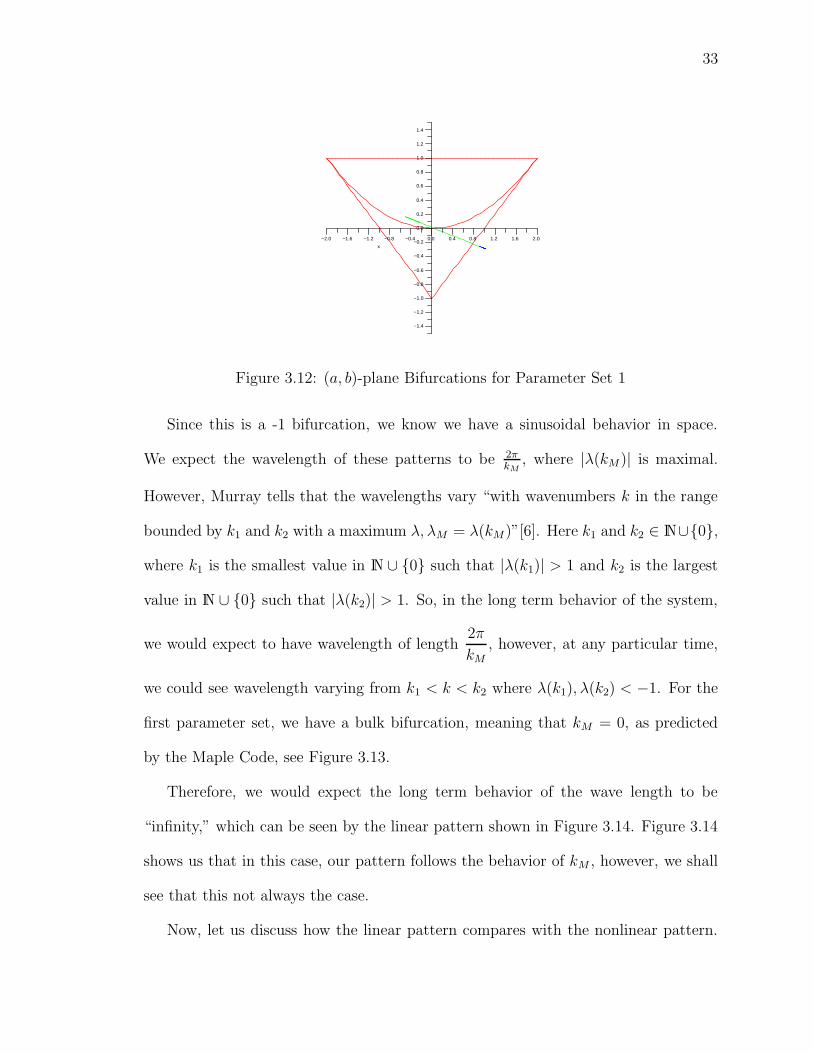
First we will begin by looking at the bifurcation diagram in the (a, b)-plane. As you
can see by Figure 3.12, the λ curve intersects the right side of the triangle.
33
−0.2
−0.4
−0.6
−0.8
−1.0
−0.8
−1.2
−1.4
x
−1.6 2.01.61.20.80.4
0.8
−0.4−1.2
1.0
0.0
−2.0
1.2
0.0
0.2
0.4
1.4
0.6
Figure 3.12: (a, b)-plane Bifurcations for Parameter Set 1
Since this is a -1 bifurcation, we know we have a sinusoidal behavior in space.
We expect the wavelength of these patterns to be 2πkM
, where |λ(kM)| is maximal.
However, Murray tells that the wavelengths vary “with wavenumbers k in the range
bounded by k1 and k2 with a maximum λ, λM = λ(kM)”[6]. Here k1 and k2 ∈ N∪0,
where k1 is the smallest value in N ∪ 0 such that |λ(k1)| > 1 and k2 is the largest
value in N ∪ 0 such that |λ(k2)| > 1. So, in the long term behavior of the system,
we would expect to have wavelength of length2π
kM
, however, at any particular time,
we could see wavelength varying from k1 < k < k2 where λ(k1), λ(k2) < −1. For the
first parameter set, we have a bulk bifurcation, meaning that kM = 0, as predicted
by the Maple Code, see Figure 3.13.
Therefore, we would expect the long term behavior of the wave length to be
“infinity,” which can be seen by the linear pattern shown in Figure 3.14. Figure 3.14
shows us that in this case, our pattern follows the behavior of kM , however, we shall
see that this not always the case.
Now, let us discuss how the linear pattern compares with the nonlinear pattern.

34
k
1.1
0.9
0.7
12.5
0.3
0.1
1.2
1.0
0.8
0.6
15.0
0.5
0.4
0.2
10.07.55.02.50.0
Figure 3.13: The eigenvalues for Parameter Set 1
Figure 3.14: Linear -1 Bifurcation for Parameter Set 1
The nonlinear pattern can be seen in Figure 3.15
Finally, we can see how long the linear pattern approximates the nonlinear pattern
by examining Figure 3.16
As you can see, the linear model for this parameter set approximates the nonlinear
one for about 47 time iterates. Now we will examine the second parameter set.
3.3.2 Parameter Set 2
As before, we will begin our discussion by examining the bifurcation diagram for pa-
rameter set 2 in the (a, b)-plane. Now, we want to look at the range of the eigenvalues

35
Figure 3.15: Nonlinear -1 Bifurcation for Parameter Set 1
0 5 10 15 20 25 30 35 40 45 500
0.2
0.4
0.6
0.8
1
1.2
1.4
Time
Nor
m o
f Diff
ernc
es
Difference between Linear and Nonlinear Attractor
Figure 3.16: Difference Between the Linear and Nonlinear Patterns for Parameter Set
1
of this parameter set to see what kind of pattern to expect. Figure 3.18 will show
us the range of the eigenvalues |λ| > 1. So, we can see from Figure 3.18 that we
can expect our k value to be 4 < k < 20 with kM ≈ 6. Now let us look at Figure
3.19 to see what the linear pattern actually looks like. From Figure 3.19, we see that
there are 12 vertical stripes, and by examining the linear pattern at t = 15, 16 we see
that there are exactly 6 cycles in that graph. This tell us that we have a wavelength
of 2π/6 which was predicted by Murray. Now let us examine the nonlinear pattern
and compare it to the linear pattern. We can see that the nonlinear pattern follows
exactly from the linear pattern. We see that the nonlinear pattern is period 2 in time

36
0.4
0.2
0.0
−0.2
−0.4
0.8
−0.6
−0.8
−1.0
−1.2
−0.8
−1.4
−1.6 2.0
1.4
1.0
0.8
1.20.0 0.4−0.4−1.2 1.6
0.6
−2.0
1.2
Figure 3.17: (a, b)-plane Bifurcations for Parameter Set 2
0.75
14
0.5
0.25
0.0
1086 244
1.5
2 120 2016 18
1.0
1.25
k
22
1.75
Figure 3.18: The eigenvalues for Parameter Set 2
and has 6 cycles in the graph. Now, let us consider the length of time that the linear
model approximates the nonlinear model for this parameter set. Figure 3.21 shows
that we can expect the linear pattern to approximate the nonlinear pattern for about
the first 20 time iterates. Now we shall examine how the patterns can change based
on a change in initial conditions, but leaving the parameters unchanged.

37
0 1 2 3 4 5 6 7−0.2
−0.15
−0.1
−0.05
0
0.05
0.1
0.15
Space
Linear Model t = 15,16
t=15
t=16
Figure 3.19: Linear -1 Bifurcation for Parameter Set 2, Linear pattern at t = 15, 16
0 1 2 3 4 5 6 7−0.6
−0.5
−0.4
−0.3
−0.2
−0.1
0
0.1
0.2
0.3
0.4Nonlinear Model t = 750,751
Space
t=750data2
Figure 3.20: Nonlinear -1 Bifurcation for Parameter Set 2, Nonlinear pattern at
t = 750, 751
3.3.3 Variation of Initial Conditions
If we vary the initial conditions of parameter set 1, we can see a different pattern
than the one shown in Figure 3.14. We know from Figure 3.13 that it is possible to
have k values ranging from 0 to about 30. Now let us examine Figure 3.22. From this
figure we can see that we have one cycle, implying that in this case we have k = 1.
Therefore, just as in the +1 bifurcations, we can see a different eigenvalue from the
most dominate one control how the pattern is formed for certain initial conditions.

38
0 5 10 15 20 250
0.2
0.4
0.6
0.8
1
1.2
1.4
1.6
1.8
2
Time
Nor
m o
f Diff
ernc
es
Difference between Linear and Nonlinear Attractor
Figure 3.21: Difference Between the Linear and Nonlinear Pattern for Parameter Set
2
0 1 2 3 4 5 6 7−1.5
−1
−0.5
0
0.5
1
1.5x 10
4 Linear Model t = 90,91
Space
t=90data2
Figure 3.22: Linear -1 Bifurcation for Parameter Set 1 with a Different Pattern
3.4 Complex Bifurcation
Complex bifurcations occur when the λ curve intersects the top part of the triangle
in Figure 3.1. To understand the patterns these types of bifurcations create, let us
take a look at the parameter values in Table 3.3.
Table 3.3: Parameter Values for Complex Bifurcations
Set Number θE θI αE αI σE σI δ γ νE νI
1 2.1 3.0 10.0 9.0 0.1 0.2 0.7 0.8 0.7 0.72 0.2 0.3 20.0 7.0 1.3 0.7 0.4 0.905 1.5 1.5
Since we have a complex bifurcation, then we have a λt = rteiθt, θ 6= 0, θ 6= π.

39
Since |λ| > 1, then r > 1, so we see exponential growth. However, since this is a
complex bifurcation, arg(λ) > 0. This tell us that the pattern travels on the unit
circle by the amount arg(λ). Also, we still have the spatial variations as we he had in
+1 and -1 bifurcations. Because of this, we expect to see a spatio-temporal pattern[3].
Now, let us take a look at parameter set 1.
3.4.1 Parameter Set 1
First, we will look at the bifurcation graph for this parameter set. It can be seen in
Figure 3.23. Now we will calculate the spatial variations we should expect from this
0.4
−1.6 1.6
0.2
0.0
−0.2
−0.4
−0.6
−0.8
−1.0
−1.2
−1.4
0.0−0.8
1.4
1.0
0.8
2.01.20.4−0.4−1.2
0.6
0.8−2.0
1.2
Figure 3.23: (a, b)-plane Bifurcations for Parameter Set 1
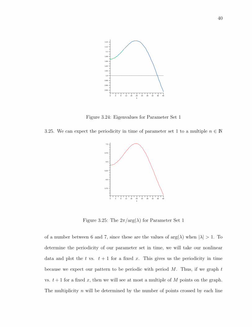
parameter set. From figure 3.24 we see that k1 = 0 and k2 ≈ 36 with kM ≈ 22. Thus,
we could see wavelengths anywhere from length “∞” to 2π/36. However, since we
have a complex bifurcation, we must also be concerned with the arg(λ). The arg(λ)
will determine the periodicity we see in time. We use the Maple code to compute
the arg(λ) and use this to compute the expected periodicity in time of this particular
pattern. The range of periodicity with respect to the k values can be seen in Figure
40
1.1
1.12
1.02
1.04
24
0.94
0.96
32
k
40
1.14
36
1.08
1.06
28
1.0
0.98
201612840
Figure 3.24: Eigenvalues for Parameter Set 1
3.25. We can expect the periodicity in time of parameter set 1 to a multiple n ∈ N
6.75
20
6.25
k
40363228
7.0
24
6.5
6.0
16
5.75
12840
Figure 3.25: The 2π/arg(λ) for Parameter Set 1
of a number between 6 and 7, since these are the values of arg(λ) when |λ| > 1. To
determine the periodicity of our parameter set in time, we will take our nonlinear
data and plot the t vs. t + 1 for a fixed x. This gives us the periodicity in time
because we expect our pattern to be periodic with period M . Thus, if we graph t
vs. t + 1 for a fixed x, then we will see at most a multiple of M points on the graph.
The multiplicity n will be determined by the number of points crossed by each line

41
segment +1 in the t vs. t + 1 graph. Figure 3.26 shows us the t vs. t + 1 plot for
parameter set 1. From Figure 3.26, we see that no line segment crosses any points,
−3 −2 −1 0 1 2 3 4−3
−2
−1
0
1
2
3
4t vs. t+1 at x = 2*pi/40
t
t+1
Figure 3.26: Periodicity of Parameter Set 1
thus the multiplicity of our parameter set is n = 1. Now, counting the number nodes
in the graph, we see that the periodicity of this parameter set in time is slightly more
than 6, which is what we would expect.
Let us see if this parameter set behaves as expected. Figure 3.27 show the linear
pattern generated by parameter set 1, along with the 3 values u(t, Ω) for t = 550, 551,
and 552. We can see that there are 19 cycles in the linear pattern, cooresponding
0 1 2 3 4 5 6 7−1.5
−1
−0.5
0
0.5
1
1.5x 10
29
Space
Linear Model t = 550,551,552
t=550t=551t=552
Figure 3.27: Linear Complex Bifurcation for Parameter Set 1, Linear Pattern at
t = 550, 551, 552
to a wavelength of 2π/19 which is in the predicted range. Also, we see that Figure

42
3.27 varies both spatially and temporally as expected. Now, let us examine the
nonlinear pattern and see if it has the behavior we expect. Figure 3.28 has a spatio-
0 1 2 3 4 5 6 7−4
−3
−2
−1
0
1
2
3
4
5Nonlinear Model t = 900,901,902
Space
Figure 3.28: Nonlinear Complex Bifurcation for Parameter Set 1, Nonlinear Pattern
at t = 900, 901, 902
temporal pattern as expected. We can see that there are 24 cycles, cooresponding to
wavelengths of 2π/24, which differs from the linear pattern. However, this wavelength
is still well within the expected range of values. However, other than the difference
in wavelengths, the linear and nonlinear patterns are identical.
Now we will look how long the linear pattern approximates the nonlinear pattern.
Let us take a look at Figure 3.29. Thus, this linear pattern approximates the nonlinear
0 10 20 30 40 50 60 70 800
0.2
0.4
0.6
0.8
1
1.2
1.4
Time
Nor
m o
f Diff
ernc
es
Difference between Linear and Nonlinear Attractor
Figure 3.29: Difference Between the Linear and Nonlinear Patterns for Parameter Set
1
43
pattern for about 70 time iterates in this parameter set. Now, let us look at some
interesting patterns that emerge from this parameter set.
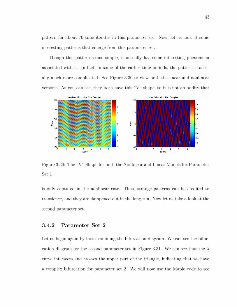
Though this pattern seems simple, it actually has some interesting phenomena
associated with it. In fact, in some of the earlier time periods, the pattern is actu-
ally much more complicated. See Figure 3.30 to view both the linear and nonlinear
versions. As you can see, they both have this “V” shape, so it is not an oddity that
Figure 3.30: The “V” Shape for both the Nonlinear and Linear Models for Parameter
Set 1
is only captured in the nonlinear case. These strange patterns can be credited to
transience, and they are dampened out in the long run. Now let us take a look at the
second parameter set.
3.4.2 Parameter Set 2
Let us begin again by first examining the bifurcation diagram. We can see the bifur-
cation diagram for the second parameter set in Figure 3.31. We can see that the λ
curve intersects and crosses the upper part of the triangle, indicating that we have
a complex bifurcation for parameter set 2. We will now use the Maple code to see
44
0.4
0.2
0.0
−0.2
−0.4
−0.6
−0.8
−1.2
1.60.80.0−0.8−1.6 2.0
1.4
1.0
0.8
1.20.4−0.4−1.2
−1.0
−1.4
−2.0
0.6
1.2
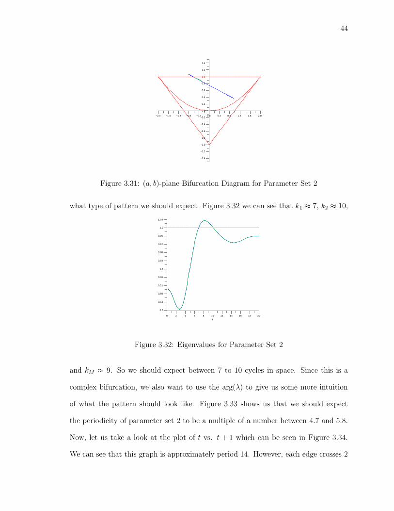
Figure 3.31: (a, b)-plane Bifurcation Diagram for Parameter Set 2
what type of pattern we should expect. Figure 3.32 we can see that k1 ≈ 7, k2 ≈ 10,
1.0
0.92
0.84
0.76
14
0.6
k
18
1.04
0.96
0.88
20
0.8
0.72
16
0.68
0.64
121086420
Figure 3.32: Eigenvalues for Parameter Set 2
and kM ≈ 9. So we should expect between 7 to 10 cycles in space. Since this is a
complex bifurcation, we also want to use the arg(λ) to give us some more intuition
of what the pattern should look like. Figure 3.33 shows us that we should expect
the periodicity of parameter set 2 to be a multiple of a number between 4.7 and 5.8.
Now, let us take a look at the plot of t vs. t + 1 which can be seen in Figure 3.34.
We can see that this graph is approximately period 14. However, each edge crosses 2

45
7.5
4.5
2.5
2.5
k15.012.510.0
5.0
4.0
5.0
3.5
3.0
0.0
Figure 3.33: The 2π/arg(λ) for Parameter Set 2
−4 −3 −2 −1 0 1 2 3 4−4
−3
−2
−1
0
1
2
3
4
t
t+1
t vs. t+1 at x = 2*pi/1024
Figure 3.34: Periodicity of Parameter Set 2
points, thus the multiplicity of this graph is n = 3. Since 4.7 · 3 = 14.1 ≈ 14, then we
can see that the Maple code correctly predicted the periodicity of parameter set 2.
Now, we will normally we would examine the linear pattern, but there is a problem
with the linear code for this parameter set. We will explain more about this later on.
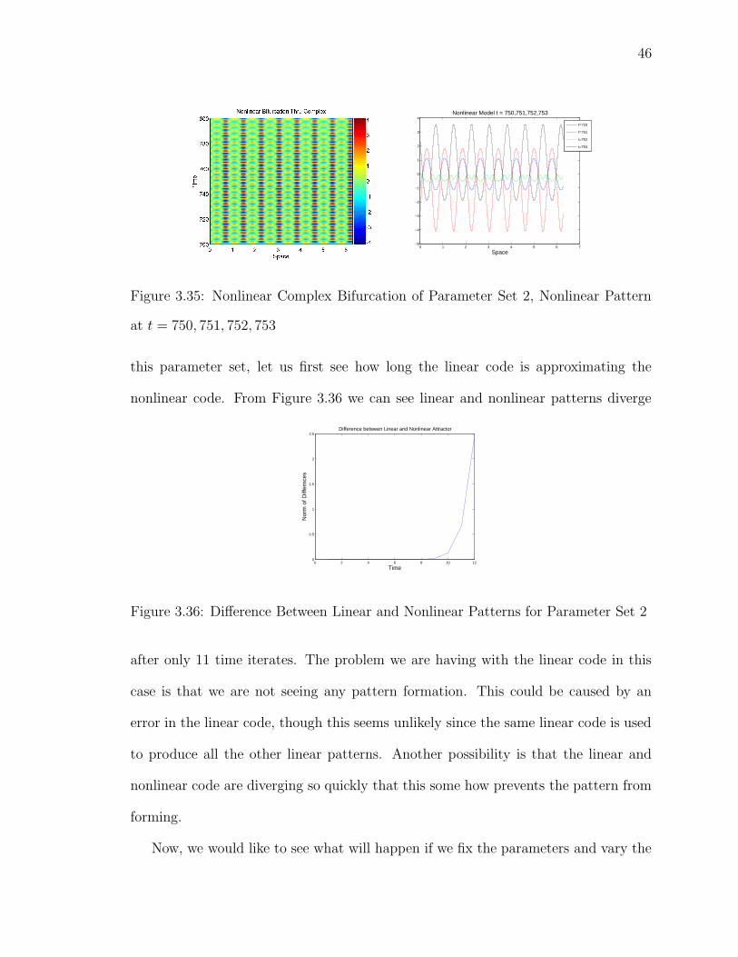
For now, let us examine the nonlinear pattern. Figure 3.35 shows us the nonlinear
pattern along with the graph for fixed time periods 750, 751, 752, and 753. From
the graph of the fixed time periods, we can see that there are 8 cycles in the graph,
cooresponding to a wavelength of 2π/8 which is in the expected range.
To understand the problem we are having with generating the linear pattern for
46
0 1 2 3 4 5 6 7−5
−4
−3
−2
−1
0
1
2
3
4
Space
Nonlinear Model t = 750,751,752,753
t=750
t=751
t=752
t=753
Figure 3.35: Nonlinear Complex Bifurcation of Parameter Set 2, Nonlinear Pattern
at t = 750, 751, 752, 753
this parameter set, let us first see how long the linear code is approximating the
nonlinear code. From Figure 3.36 we can see linear and nonlinear patterns diverge
0 2 4 6 8 10 120
0.5
1
1.5
2
2.5
Time
Nor
m o
f Diff
ernc
es
Difference between Linear and Nonlinear Attractor
Figure 3.36: Difference Between Linear and Nonlinear Patterns for Parameter Set 2
after only 11 time iterates. The problem we are having with the linear code in this
case is that we are not seeing any pattern formation. This could be caused by an
error in the linear code, though this seems unlikely since the same linear code is used
to produce all the other linear patterns. Another possibility is that the linear and
nonlinear code are diverging so quickly that this some how prevents the pattern from
forming.
Now, we would like to see what will happen if we fix the parameters and vary the

47
initial conditions.
3.4.3 Variation of Initial Conditions
We are going to show that for a particular parameter set, a complex bifurcation can
have different periodicity in time. To see how this occurs, let us look at Figure 3.37
Table 3.4: Parameter Values for Complex Bifurcations with Period 5 and 19
Set Number θE θI αE αI σE σI δ γ νE νI
1 0.2 0.3 20.0 7.0 1.3 0.7 0.4 0.87 1.5 1.5
which show us the eigenvalues for this parameter set as well as the 2π/arg(λ). We
87
0.96
10
0.88
k
0.8
1.0
93
0.64
2 11
0.92
6
0.84
0.76
4
0.72
0.68
0.6
10 5 12 873
4.5
3.5
1
2.5
654
5.0
4.0
2
3.0
0k
109 11 12
Figure 3.37: Eigenvalues and 2π/arg(λ) for the Parameter Set in Table 3.4
can see that the only k values that gives us |λ(k)| > 1 are k = 7, 8, 9. Also, from the
graph of 2π/arg(λ) we see that we should expect the periodicity of this parameter
set to be approximately a multiple of a number between 4.8 to 5.8. For the first set
of initial conditions, we can see the periodicity based on these initial conditions in
Figure 3.38. We can see that the multiplicity is n = 1 and we see a period 5 pattern
as expected. Now, let us take a look at Figure 3.39 to see the periodicity of this

48
−2 −1.5 −1 −0.5 0 0.5 1 1.5−2
−1.5
−1
−0.5
0
0.5
1
1.5t vs. t+1 at x = 2*pi/400
t
t+1
Figure 3.38: Initial Conditions which are Period 5 in Time.
parameter set for the second set of initial conditions. We finish this discussion by
−2 −1.5 −1 −0.5 0 0.5 1 1.5 2−2
−1.5
−1
−0.5
0
0.5
1
1.5
2t vs. t+1 at x = 2*pi/400
t
t+1
Figure 3.39: Initial Conditions which are Period 19 in Time.
We can see that the periodicity of this parameter set for the second set of initial
conditions to be approximately period 19. We can see that each edge pass through 3
nodes, giving us a multiplicity of n = 4. This is consistent with the Maple code
since 4.8 · 4 = 19.32 ≈ 19.
examining the nonlinear patterns of this parameter set for the cooresponding initial
conditions. These patterns are seen in Figure 3.40. Now, we will consider what
happens when we have multiple bifurcations.

49
Figure 3.40: Patterns generated for γ = .87 for a pattern which is period 5 in and
period 19 in time.
3.5 Multiple Bifurcations
A parameter set which has λ curve in the (a, b)− plane which intersects the triangle
in Figure 3.1 on multiple sides is said to have multiple bifurcations. We will not
be doing an in-depth analysis of these types of bifurcations. Instead, we will show
some of the interesting patterns these types of bifurcations creates. The first type of
bifurcation we will see is a bifurcation through complex and -1.
3.5.1 Bifurcations thru Complex and -1
The parameter set that produced the pattern that we will be examining can be seen
in Table 3.5. The nonlinear pattern for this parameter set can seen in Figure 3.41
Table 3.5: Parameter Values for Bifurcation which are both Complex and -1
Set Number θE θI αE αI σE σI δ γ νE νI
1 0.2 0.3 19.0 10.0 1.0 0.2 0.2 0.9 1.0 1.0
Now, we will be examining a pattern created from a +1 and -1 bifurcations.

50
Figure 3.41: Nonlinear Bifurcation thru Complex and -1
3.5.2 Bifurcations thru +1 and -1
The parameter set used to generate the pattern we will be viewing can be seen in
Table 3.6. The nonlinear pattern for this parameter set can be seen in Figure 3.42.
Table 3.6: Parameter Values for Bifurcation which are both +1 and -1
Set Number θE θI αE αI σE σI δ γ νE νI
1 0.1 0.0 6.0 8.0 0.1 0.2 0.1 0.0 3.0 3.0
We conclude this thesis with a discuss of the rate of divergence of the linear and
Figure 3.42: Nonlinear Bifurcation thru +1 and -1
nonlinear model.

51
3.6 Analysis of the Rate of Divergence
We will now consider the rate of divergence of the linear model with respect to the
nonlinear model. To do this, we will fix all parameters except for a single parameter
which will allow us to have an unstable solution bifurcate from a stable solution
to a unstable solution. Table 3.7 shows the parameter set we will be using. This
Table 3.7: Parameter Values for Bifurcation which are both +1 and -1
Set Number θE θI αE αI σE σI δ γ νE νI
1 2.1 3.0 10.0 9.0 0.1 0.2 0.7 variable 0.7 0.7
parameter set is the same as parameter set 1 in Table 3.3, except we are varying γ.
The bifurcation remains a complex bifurcation as we vary γ. Figures 3.43 and 3.44
show us how the λ curve moves through the bifurcation as we vary γ. The plot
−0.20.8
−0.4
−0.6
−0.8
−1.0
−1.2
−1.4
0.0
k
−0.8 2.0−1.6 1.61.2
0.8
0.4−0.4−1.2
1.0
0.0
−2.0
0.2
0.4
1.2
1.4
0.6
−0.20.8
−0.4
−0.6
−0.8
−1.0
−1.2
−1.4
0.0
x
−0.8 2.0−1.6 1.61.2
0.8
0.4−0.4−1.2
1.0
0.0
−2.0
0.2
0.4
1.2
1.4
0.6
Figure 3.43: Complex Bifurcations for γ = .463 and γ = .7
the || · ||∞ of the differences of the linear and nonlinear model with respect to γ can
be seen in Figure 3.45. We see an exponential decay in the amount of time that the
linear and nonlinear models approximate each other. This is because as the λ curves
moves further through the complex bifurcation, the dominant eigenvalue,call it λM ,
increases in modulus. Thus, the rate at which the linear model diverges from the

52
0.4
−1.6 1.6
0.2
0.0
−0.2
−0.4
−0.6
−0.8
−1.0
−1.2
−1.4
0.0−0.8
1.4
1.0
0.8
2.01.20.4−0.4−1.2
0.6
0.8−2.0
1.2
0.4
0.2
0.0
−0.2
−0.4
0.8
−0.6
−0.8
−1.0
−1.2
−0.8
−1.4
−1.6 2.0
1.4
1.0
0.8
1.61.20.0 0.4−0.4−1.2
0.6
−2.0
1.2
Figure 3.44: Complex Bifurcation for γ = .8 and γ = .999
nonlinear model increases exponentially as γ increases. In fact, this holds true for
any type of bifurcation since the further the λ curve moves through the bifurcation,
the large the modulus of the maximum eigenvalues become.
0.4 0.5 0.6 0.7 0.8 0.9 10
200
400
600
800
1000
1200
1400
1600
1800
gamma values
perio
d of
tim
e lin
ear
appr
oxim
ates
non
linea
r
Period of time linear approximates nonlinear w.r.t. gamma
Figure 3.45: How || · ||∞ of the Difference of the Linear and Nonlinear Model varies
with respect to γ

Bibliography
[1] Kathleen T. Alligood, Tim D. Sauer, and James A. Yorke. Chaos: An Introduction
to Dynamical Systems. Springer, 1996.
[2] Thomas H. Cormen, Charles E. Leiserson, Ronald L. Rivest, and Clifford Stein.
Introduction to Algorithms, 2nd Edition. McGraw-Hill, 2001.
[3] Bard Ermentrout, John Campbell, and George Oster. A model for shell patterns
based on neural activity. The Veliger, 28(4):369–388, April 1986.
[4] Gerald B. Folland. Real Analysis: Modern Techniques and Their Applications,
2nd Edition. Wiley Inter-Science, 1999.
[5] Micheal Heath. Scientific Computing: An Introductory Survey, 2nd Edition.
McGraw-Hill, 2002.
[6] J.D.Murray. Mathematical Biology, 2nd Edition. Springer, Berlin, 1993.
[7] Paul A. Meglitsch. Invertebrate Zoology. Oxford University Press, 1967.
[8] Giancarlo Paganelli. Coneshells. http://www.coneshell.net/images/sh shell.jpg.
53

54
Appendix A: Source Code
A.1 C++ Code
/***************************************************************************
* Copyright (C) 2005 by Tyler M. White *
* *
* This program is free software; you can redistribute it and/or modify *
* it under the terms of the GNU General Public License as published by *
* the Free Software Foundation; either version 2 of the License, or *
* (at your option) any later version. *
* *
* This program is distributed in the hope that it will be useful, *
* but WITHOUT ANY WARRANTY; without even the implied warranty of *
* MERCHANTABILITY or FITNESS FOR A PARTICULAR PURPOSE. See the *
* GNU General Public License for more details. *
* *
* You should have received a copy of the GNU General Public License *
* along with this program; if not, write to the *
* Free Software Foundation, Inc., *
* 59 Temple Place - Suite 330, Boston, MA 02111-1307, USA. *
***************************************************************************/
/*Description: This program was written by Tyler White to be used in his
/* Honors Thesis in Mathematics. This program implements an

55
/* an algorithm used to produce shell patterns. The algorithm
/* this model was based on was original proposed by Ermentrout,
/* Campbell, and Oster in 1986. This code not only generates the
/* the nonlinear patterns, but also computes the linear patterns
/* based on the linearization of the nonlinear model and also
/* computes the infinity norm of the differences between the
/* linear and nonlinear patters.*/
#ifdef HAVE_CONFIG_H
#include <config.h>
#endif
#include <iostream> //for basic output to console
#include <math.h> //for the basic C++ math libraries
#include <fstream> //for the file stream class to write to files
#include <vector> //for the Standard Template Library vector container
#include <fftw3.h> //for the fast fourier transform library
#include <algorithm> //for the Standard Template Library algorithms
#include <time.h> //to get the system time
#include <stdlib.h> //basic library functions such as rand()
#include <cstdlib>
using namespace std;
#define PI 3.14159265358979323846 //store highly accurate value for pi.
#define pwr 12 //used to set the size of the domain which will be 2^pwr
#define p 4

56
/***********************************************************************/
/*This section is the functions used by main to interface with the rest*/
/*of the program */
void getInput();
//this function is used to get the input from the user
/* */
void patternGen();
//this function is the interface between main and the computation part
//of the program
/* */
void initializationVariables();
//this function initializes all the variables
void cleanUp();
//this function cleans up the variables at the end of the program
/***********************************************************************/
/*************************************************************************/
/*these functions are part of the original formulations of the model */
double wE( double x );
//This function evaluates wE for all values of x in the domain
double wI( double x );
//This function evaluates wI for all values of x in the domain
double SE( double x );
//This function evaluates SE for all values of Pt(x) of x in the domain
double SI( double x );

57
//This function evaluates SI for all values of Pt(x) of x in the domain
double S( double x_E, double x_I );
//This function calls SE and SI and takes their difference and returns that
/**************************************************************************/
/***********************************************************************/
/*Functions used in determining the homogenous equilibrium solution */
/* */
double equationNewton(double x);
//Part of newtons method, basically the f(x) of newtons method */
/* */
double equationNewtonPrime(double x);
//Part of newtons method, basically the fprime(x) of newtons method */
/* */
double newtonMethodP0(double x);
//xt_p_1 = xt - f(x)/fprime(x) */
/* */
void computeEquilibrium();
/*uses fixed point iteration and newtons method to come up with a */
/*solution. */
/*These are the variables used for calculating the equilibrium solution*/
double equilibrium = -0.3938;
double precision;
double accuracy = 8;
/***********************************************************************/
/***********************************************************************/

58
/*these functions are speifically used in the linearization */
/* calculations*/
double SprimeE( double x );
//this function determines the derivative of SE for a given value of x
double SprimeI( double x );
//this function determines the derivative of SI for a given value of x
void computeL0();
//this function commputes the convolution of ut and wE and wI and uses
//this to compute L0
/***********************************************************************/
/************************************************************************/
/*these are the auxillery fuctions which perform simple calculations */
/*help make the code more modular */
void arrayCpy( double a[], double b[] );
//Function that copies the values of array b into array a
void computeConvolution( fftw_plan&, fftw_complex[],
fftw_complex[], fftw_complex[] );
//This is used for computing the convolution operator
//It assumes that the variables have already been transformed into
//Fourier Space.
double infinity_norm(double*, double*);
//This uses the infinity norm to calculate the distance between two vectors
//in R^n, the first parameter is the Pt values and the second parameter is
//the Ut value.

59
double rel_norm(double*, double*, double);
/*************************************************************************/
/**********************************************************/
/*These are the main parameters for this program */
double theta_E = .2;
double theta_I = 0.3;
double alpha_E = 20;
double alpha_I = 7;
double sigma_E = 1.3;
double sigma_I = .7;
double gamma1 = .85;
double delta = 0.4;
double nu_E = 1.5;
double nu_I = 1.5;
double q_E = alpha_E*4/(93*sigma_E); //parameter which depends on alpha,
//p, and sigma
double q_I = alpha_I*4/(93*sigma_I); //parameter which depends on alpha,
//p, and sigma
const int N = 1 << pwr; //evalutes 2^pwr using the bitshift operator
int max_time = 2000; //defines the length of the time interval, so
//time goes from 0 to max_time
/**********************************************************/
/************************************************************************/
/*These are the fourier transform plans used to execute */
/*the fourier tranforms */

60
fftw_plan fft_wE; //for the fourier transform of wE(x)
fftw_plan fft_Pt; //for the fourier transform of Pt(x)
fftw_plan fft_wI; //for the fourier transform of wI(x)
fftw_plan fft_Ut;
fftw_plan ifft_SwE; //for the fourier transform of the conv of
//SE[Et(x)]
fftw_plan ifft_SwI; //for the fourier transform of the conv of
//SI[It(x)]
fftw_plan ifft_SwE1; //for the fourier transform of the conv of
//SE[Et(x)]
fftw_plan ifft_SwI1; //for the fourier transform of the conv of
//SI[It(x)]
/***********************************************************************/
/***********************************************************************/
/*These are variables used in the fourier transforms for input and output*/
double *in_wE; //input for the fft of wE(x)
double *in_wI; //input for the fft of wI(x)
double *in_Ut;
fftw_complex *out_Ut;
fftw_complex *out_wE; //output for the fft of wE(x)
fftw_complex *out_wI; //output for the fft of wI(x)
double *in_Pt; //input for the fft of Pt(x)
fftw_complex *out_Pt; //output for the fft of Pt(x)
fftw_complex *in_SwE; //input for the conv of Pt(x) and wE(x)
double *out_SwE; //output for the conv of Pt(x) and wE(x)
fftw_complex *in_SwI; //input for the conv of Pt(x) and wI(x)

61
double *out_SwI; //output for the conv of Pt(x) and wI(x)
fftw_complex *in_SwE1; //input for the conv of Pt(x) and wE(x)
double *out_SwE1; //output for the conv of Pt(x) and wE(x)
fftw_complex *in_SwI1; //input for the conv of Pt(x) and wI(x)
double *out_SwI1; //output for the conv of Pt(x) and wI(x)
/**************************************************************************/
/**************************************************************************/
//these variables are used in the actual computations for Pt, Ut, and L0t
double *Pt; //the pigmentation from 2 iterations ago
double *Pt_p_1; //the pigmentation from 1 iteration ago
double *Pt_p_2; //the currently calculated pigmentation
double *Ut;
double *Ut_p_1;
double *Ut_p_2;
double *L0;
double *L0t;
double *L0t_p_1;
double *L0t_p_2;
double x_coor[N];
double temp_SwE[N];
double temp_SwE1[N];
double temp_SwI1[N];
double temp_SwI[N];
/**************************************************************************/
double diff = 2*PI/(N-1); //Sets up the difference between each

62
//x values, all equall spaced
ofstream *file = NULL; //used create the file the data
//is stored in.
ofstream *file1 = NULL;
ofstream *file2 = NULL;
ofstream *file3 = NULL;
vector<double*> data_store; //a vector to store all pigmation
//patterns for all time iterations
vector<double*> data_store_1; //a vector to store all the
//linearization values
vector<double> dist; //stores the infinity norm for
//each iteration
vector<double> norm_dist;
bool testflag = true;
enum comp real, imaginary ; //this is used to help me keep track of the
//multiplication of complex numbers.
int main(int argc, char *argv[])
string yes_no = "";
srand((int)time(NULL));
initializationVariables();
do
cout << "here again" << endl;
getInput();
computeEquilibrium();

63
patternGen();
cout << "Continue?[y/n]: ";
cin >> yes_no;
cout << "here" << endl;
while( yes_no[0] != ’y’ && yes_no[0] != ’n’ )
cout << "Invalid Entry" << endl
<< "Continue?[y/n]:";
cin >> yes_no;
while( yes_no[0] != ’n’ );
cleanUp();
return 0;
/*The main functions******************************************************/
void initializationVariables()
cerr << "Variable Initialization: ";
L0 = (double*)fftw_malloc(N*sizeof(double));
L0t = (double*)fftw_malloc(N*sizeof(double));
L0t_p_1 = (double*)fftw_malloc(N*sizeof(double));
cerr << "*";
L0t_p_2 = (double*)fftw_malloc(N*sizeof(double));
in_Ut = (double*)fftw_malloc(N*sizeof(double));
out_Ut = (fftw_complex*)fftw_malloc(N*sizeof(fftw_complex));
cerr << "*";

64
in_wE = (double*)fftw_malloc(N*sizeof(double));
in_wI = (double*)fftw_malloc(N*sizeof(double));
out_wE = (fftw_complex*)fftw_malloc(N*sizeof(fftw_complex));
cerr << "*";
out_wI = (fftw_complex*)fftw_malloc(N*sizeof(fftw_complex));
in_Pt = (double*)fftw_malloc(N*sizeof(double));
out_Pt = (fftw_complex*)fftw_malloc(N*sizeof(fftw_complex));
cerr << "*";
in_SwE = (fftw_complex*)fftw_malloc(N*sizeof(fftw_complex));
out_SwE = (double*)fftw_malloc(N*sizeof(double));
in_SwI = (fftw_complex*)fftw_malloc(N*sizeof(fftw_complex));
cerr << "*";
out_SwI = (double*)fftw_malloc(N*sizeof(double));
in_SwE1 = (fftw_complex*)fftw_malloc(N*sizeof(fftw_complex));
out_SwE1 = (double*)fftw_malloc(N*sizeof(double));
cerr << "*";
in_SwI1 = (fftw_complex*)fftw_malloc(N*sizeof(fftw_complex));
out_SwI1 = (double*)fftw_malloc(N*sizeof(double));
Ut = (double*)fftw_malloc(N*sizeof(double));
cerr << "*";
Ut_p_1 = (double*)fftw_malloc(N*sizeof(double));
Ut_p_2 = (double*)fftw_malloc(N*sizeof(double));
Pt = (double*)fftw_malloc(N*sizeof(double));
cerr << "*";
Pt_p_1 = (double*)fftw_malloc(N*sizeof(double));
Pt_p_2 = (double*)fftw_malloc(N*sizeof(double));
fft_wE = fftw_plan_dft_r2c_1d(N, in_wE, out_wE, FFTW_EXHAUSTIVE);

65
cerr << "*";
fft_wI = fftw_plan_dft_r2c_1d(N, in_wI, out_wI, FFTW_EXHAUSTIVE);
fft_Pt = fftw_plan_dft_r2c_1d(N, in_Pt, out_Pt, FFTW_EXHAUSTIVE);
fft_Ut = fftw_plan_dft_r2c_1d(N, in_Ut, out_Ut, FFTW_EXHAUSTIVE);
cerr << "*";
ifft_SwE = fftw_plan_dft_c2r_1d(N, in_SwE, out_SwE, FFTW_EXHAUSTIVE);
ifft_SwI = fftw_plan_dft_c2r_1d(N, in_SwI, out_SwI, FFTW_EXHAUSTIVE);
ifft_SwE1 = fftw_plan_dft_c2r_1d(N, in_SwE1, out_SwE1, FFTW_EXHAUSTIVE);
cerr << "*";
ifft_SwI1 = fftw_plan_dft_c2r_1d(N, in_SwI1, out_SwI1, FFTW_EXHAUSTIVE);
precision = 0.5*pow(10, -1*accuracy);
cerr << endl << "Initialization Complete" << endl;
return;
void getInput()
string temp;
cerr << "Enter theta_E[" << theta_E << "]: ";
if( testflag )
testflag = false;
else
cin >> ws;
getline(cin, temp, ’\n’);
if( temp != "" )
theta_E = atof( temp.c_str() );

66
cerr << "Enter theta_I[" << theta_I << "]: ";
getline(cin, temp, ’\n’);
if( temp != "" )
theta_I = atof( temp.c_str() );
cerr << "Enter alpha_E[" << alpha_E << "]: ";
getline(cin, temp, ’\n’);
if( temp != "" )
alpha_E = atof( temp.c_str() );
cerr << "Enter alpha_I[" << alpha_I << "]: ";
getline( cin, temp, ’\n’);
if( temp != "" )
alpha_I = atof( temp.c_str() );
cerr << "Enter sigma_E[" << sigma_E << "]: ";
getline( cin, temp, ’\n’);
if( temp != "" )
sigma_E = atof( temp.c_str() );
cerr << "Enter sigma_I[" << sigma_I << "]: ";
getline( cin, temp, ’\n’);
if( temp != "" )

67
sigma_I = atof( temp.c_str() );
cerr << "Enter gamma[" << gamma1 << "]: ";
getline( cin, temp, ’\n’ );
if( temp != "" )
gamma1 = atof( temp.c_str() );
cerr << "Enter delta[" << delta << "]: ";
getline( cin, temp, ’\n’ );
if( temp != "" )
delta = atof( temp.c_str() );
cerr << "Enter nu_E[" << nu_E << "]: ";
getline( cin, temp, ’\n’ );
if( temp != "" )
nu_E = atof( temp.c_str() );
cerr << "Enter nu_I[" << nu_I << "]: ";
getline( cin, temp, ’\n’ );
if( temp != "" )
nu_I = atof( temp.c_str() );

68
void cleanUp()
fftw_free(L0);
fftw_free(L0t);
fftw_free(L0t_p_1);
fftw_free(L0t_p_2);
fftw_free(in_wI);
fftw_free(out_wE);
fftw_free(out_wI);
fftw_free(in_Pt);
fftw_free(out_Pt);
fftw_free(in_SwE);
fftw_free(out_SwE);
fftw_free(in_SwI);
fftw_free(out_SwI);
fftw_free(in_SwE1);
fftw_free(out_SwE1);
fftw_free(in_SwI1);
fftw_free(out_SwI1);
fftw_destroy_plan(fft_wE);
fftw_destroy_plan(fft_wI);
fftw_destroy_plan(fft_Pt);
fftw_destroy_plan(fft_Ut);
fftw_destroy_plan(ifft_SwE);
fftw_destroy_plan(ifft_SwI);

69
fftw_destroy_plan(ifft_SwE1);
fftw_destroy_plan(ifft_SwI1);
//end of cleanUp()
void patternGen()
cerr << "Calculations Begin: ";
q_E = alpha_E*4/(93*sigma_E);
q_I = alpha_I*4/(93*sigma_I);
Pt = (double*)fftw_malloc(N*sizeof(double));
Pt_p_1 = (double*)fftw_malloc(N*sizeof(double));
cerr << "*";
Pt_p_2 = (double*)fftw_malloc(N*sizeof(double));
if( file != NULL )
delete file;
delete file1;
delete file2;
delete file3;
file = new ofstream();
file1 = new ofstream();
file2 = new ofstream();
file3 = new ofstream();
cerr << "*";
file->open("/media/SEA__DISK/outfile.dat");
file1->open("/media/SEA__DISK/outfile1.dat");
file2->open("/media/SEA__DISK/outfile2.dat");

70
file3->open("/media/SEA__DISK/outfile3.dat");
(*file) << "%theta_E: " << theta_E << " theta_I: " << theta_I << endl
//writes variable values to file
<< "%alpha_E: " << alpha_E << " alpha_I: " << alpha_I << endl
<< "%sigma_E: " << sigma_E << " sigma_I: " << sigma_I << endl
<< "%gamma: " << gamma1 << " delta: " << delta << endl
<< "%nu_E: " << nu_E << " nu_I: " << nu_I << endl
<< "%equilibrium: " << equilibrium << endl;
(*file1) << "%theta_E: " << theta_E << " theta_I: " << theta_I << endl
<< "%alpha_E: " << alpha_E << " alpha_I: " << alpha_I << endl
<< "%sigma_E: " << sigma_E << " sigma_E: " << sigma_I << endl
<< "%gamma: " << gamma1 << " delta: " << delta << endl
<< "%nu_E: " << nu_E << " nu_I: " << nu_I << endl
<< "%equilibrium: " << equilibrium << endl;
(*file2) << "%theta_E: " << theta_E << " theta_I: " << theta_I << endl
//writes variable values to file
<< "%alpha_E: " << alpha_E << " alpha_I: " << alpha_I << endl
<< "%sigma_E: " << sigma_E << " sigma_I: " << sigma_I << endl
<< "%gamma: " << gamma1 << " delta: " << delta << endl
<< "%nu_E: " << nu_E << " nu_I: " << nu_I << endl
<< "%equilibrium: " << equilibrium << endl;
for( int i = 0; i < N; i++ )
//initializes the variables
x_coor[i] = diff*i;
Ut[i] = ((double)(rand()%1000-500.0)/500000.0);
//chooses random points
Ut_p_1[i] = ((double)(rand()%1000-500.0)/500000.0);

71
//near the equilibrium
Pt[i] = equilibrium+Ut[i]; //chooses random points
Pt_p_1[i] = equilibrium+Ut_p_1[i]; //near zero
in_wE[i] = wE(x_coor[i]);
in_wI[i] = wI(x_coor[i]);
cerr << "*";
data_store.push_back( Pt ); //stores the first
data_store.push_back( Pt_p_1 ); //and second iteration
data_store_1.push_back( Ut ); //of Pt, Ut and
data_store_1.push_back( Ut_p_1 ); //their difference
dist.push_back( infinity_norm( Pt, Ut ) );
norm_dist.push_back(rel_norm( Pt, Ut, dist[0] ) );
cerr << "*";
dist.push_back( infinity_norm( Pt_p_1, Ut_p_1 ) );
norm_dist.push_back(rel_norm( Pt_p_1, Ut_p_1, dist[1] ) );
arrayCpy( in_Pt, Pt );
arrayCpy( in_Ut, Ut );
fftw_execute(fft_Pt);
cerr << "*";
fftw_execute(fft_wE);
fftw_execute(fft_wI);
computeL0();
ofstream test;
cerr << "*";
computeConvolution( ifft_SwE, out_Pt, out_wE, in_SwE );
computeConvolution( ifft_SwI, out_Pt, out_wI, in_SwI );
72
arrayCpy( L0t, L0 );
cerr << "*";
for( int i = 2; i < max_time; i++ )
arrayCpy( in_Ut, Ut_p_1 );
arrayCpy( in_Pt, Pt_p_1 );
fftw_execute(fft_Pt);
computeL0();
arrayCpy( L0t_p_1, L0 );
arrayCpy( temp_SwE, out_SwE );
arrayCpy( temp_SwI, out_SwI );
computeConvolution( ifft_SwE, out_Pt, out_wE, in_SwE );
computeConvolution( ifft_SwI, out_Pt, out_wI, in_SwI );
for( int j = 0; j < N; j++ )
Pt_p_2[j] = S(out_SwE[j]*2*PI/(N*N),out_SwI[j]*2*PI/(N*N)) -
gamma1*Pt[j] -
delta*( S(temp_SwE[j]*2*PI/(N*N),temp_SwI[j]*2*PI/(N*N)) -
Pt_p_1[j]);
Ut_p_2[j] = L0t_p_1[j] + delta*Ut_p_1[j] - delta*L0t[j] -
gamma1*Ut[j];
data_store_1.push_back(Ut_p_2);
data_store.push_back(Pt_p_2);
dist.push_back(infinity_norm(Pt_p_2, Ut_p_2));
norm_dist.push_back(rel_norm(Pt_p_2, Ut_p_2, dist[i]));
Ut = Ut_p_1;
73
Pt = Pt_p_1;
Ut_p_1 = Ut_p_2;
Pt_p_1 = Pt_p_2;
Ut_p_2 = (double*)fftw_malloc(N*sizeof(double));
Pt_p_2 = (double*)fftw_malloc(N*sizeof(double));
arrayCpy(L0t, L0t_p_1);
cerr << "*";
for( int i = 0; i < max_time; i++ )
(*file) << dist[i] << " ";
(*file3) << norm_dist[i] << " ";
(*file) << endl;
(*file3) << endl;
for( int i = 0; i < 2000; i++ )
for( int j = 0; j < N; j++ )
(*file1) << data_store[i][j] << " ";
(*file1) << endl;
for( int i = 0; i < 2000; i++ )
for( int j = 0; j < N; j++ )
(*file2) << data_store_1[i][j] << " ";
(*file2) << endl;

74
for( int i = 0; i < max_time; i++ )
fftw_free(data_store[i]);
fftw_free(data_store_1[i]);
cerr << "*";
data_store.clear();
data_store_1.clear();
dist.clear();
norm_dist.clear();
file->close();
file1->close();
file2->close();
file3->close();
delete file1;
delete file2;
delete file;
delete file3;
file3 = NULL;
file1 = NULL;
file2 = NULL;
file = NULL;
cerr << endl << "Calculations Complete" << endl;
/*End of the main functions***********************************************/
/*These functions are used to calculate S[Pt(x)]**************************/

75
double wE( double x )
if( x > sigma_E && x < (2*PI-sigma_E) )
return 0;
else
if( x < sigma_E )
return (q_E * ( ( 1 << p) - pow(1 - cos(PI*x/sigma_E), p )));
else
return (q_E * ( ( 1 << p) -
pow(1 - cos(PI*(2*PI-x)/sigma_E), p )));
double wI( double x )
if( x > sigma_I && x < (2*PI-sigma_I) )
return 0;
else
if( x < sigma_I )
return (q_I * ( ( 1 << p ) - pow(1 - cos(PI*x/sigma_I), p )));
else
return (q_I * ( ( 1 << p ) -
pow(1 - cos(PI*(2*PI-x)/sigma_I), p )));
76
double SE( double x )
return (1/(1+exp(-1*nu_E*(x - theta_E))));
double SI( double x )
return (1/(1+exp(-1*nu_I*(x - theta_I))));
double S( double x_E, double x_I )
return (SE(x_E)-SI(x_I));
/*End of the calculations used to S[Pt(x)]*******************************/
/*This sections is used to calculate the homogenous equilibrium *********/
double newtonMethodP0( double x )
double temp;
temp = x - equationNewton( x )/equationNewtonPrime( x );
return temp;

77
double equationNewton( double x )
double temp;
temp = x - (1-delta)/(1+gamma1-delta)*(SE(alpha_E*x) - SI(alpha_I*x));
return temp;
double equationNewtonPrime( double x )
double temp;
temp = 1 - (1-delta)/(1+gamma1-delta)*(alpha_E*SprimeE(alpha_E*x)
- alpha_I*SprimeI(alpha_I*x));
return temp;
void computeEquilibrium()
double xt = 0, xt_p_1 = 0;
do
xt = xt_p_1;
xt_p_1 = newtonMethodP0(xt);
while( fabs(xt - xt_p_1) > precision );
equilibrium = xt_p_1;
cerr << "Equilibrium: " << equilibrium << endl;
/*End of the section for computing the homogenous equilibrium***************/

78
/*These functions are only used in the linearization calculations***********/
double SprimeE( double x )
return (nu_E*exp(-1*nu_E*(x - theta_E))/pow(1+exp(-1*nu_E*(x -
theta_E)),2));
double SprimeI( double x )
return (nu_I*exp(-1*nu_I*(x - theta_I))/pow(1+exp(-1*nu_I*(x -
theta_I)),2));
void computeL0()
fftw_execute(fft_Ut);
computeConvolution( ifft_SwE1, out_Ut, out_wE, in_SwE1 );
computeConvolution( ifft_SwI1, out_Ut, out_wI, in_SwI1 );
for( int i = 0; i < N; i++ )
L0[i] = SprimeE(alpha_E*equilibrium)*out_SwE1[i]*2*PI/(N*N) -
SprimeI(alpha_I*equilibrium)*out_SwI1[i]*2*PI/(N*N);
return;
/*End of the functions specifically used in the linearization calculations**/
/*These are the auxillery functions used to make the code more modular******/

79
void arrayCpy( double a[], double b[] )
for( int i = 0; i < N; i++ )
a[i] = b[i];
void computeConvolution(fftw_plan &plan, fftw_complex array1[],
fftw_complex array2[], fftw_complex array3[])
for( int i = 0; i < N; i++ )
array3[i][(int)real] = array1[i][(int)real]*array2[i][(int)real] -
array1[i][(int)imaginary]*array2[i][(int)imaginary];
array3[i][(int)imaginary] = array1[i][(int)real]*
array2[i][(int)imaginary] +
array1[i][(int)imaginary]*array2[i][(int)real];
fftw_execute(plan);
double infinity_norm(double *pt, double *ut)
double maximum = 0;
for( int i = 0; i < N; i++ )
maximum = max(fabs((pt[i]-equilibrium)-ut[i]), maximum) ;
return maximum;

80
double rel_norm(double *pt, double *ut, double numerator)
double maximum = 0;
for( int i = 0; i < N; i++ )
maximum = max(fabs(ut[i]), maximum);
return numerator/maximum;
/**************************************************************************/
A.2 Maple Code
> restart;
> p:=4;thetae:=4;thetai:=3.3;alpe:=15; alpi:=13;sigmaE:=1.3;
sigmaI:=.4;gam:=.2; delta:=.1; vue:=.4; vui:=.4;
> plot([sqrt(gam)+del, 1+gam/(1+del), 1+gam/(1-del),
(1-gam)/del],del=0..1,y=0..2, legend=["1","2","3","4"]);
> sqrt(gam)+delta; 1+gam/(1+delta); 1+gam/(1-delta); (1-gam)/delta;
> f1:=2^p-(1-cos(Pi*x/sigmaE))^p;
> f2:=2^p-(1-cos(Pi*x/sigmaI))^p;
> qE:=alpe/int(f1,x=-sigmaE..sigmaE);
> qI:=alpi/int(f2,x=-sigmaI..sigmaI);
> we:=f1*qE; wi:=f2*qI;
> int(we,x=-sigmaE..sigmaE);int(wi,x=-sigmaI..sigmaI);
> plot(we,wi,x=-sigmaE..sigmaE);
> evalf(subs(x=sigmaE/2,we));evalf(subs(x=sigmaI/2,wi));

81
> plot(wi,x=-sigmaI..sigmaI);
> fte:=(int(we*exp(I*k*x),x=-sigmaE..sigmaE)):
> fti:=(int(wi*exp(I*k*x),x=-sigmaI..sigmaI)):
> evalf(subs(k=1.00001,fte));
> plot(fte,fti,k=0..100);
> se:=x->1/(1+exp(-vue*(x-thetae)));
> si:=x->1/(1+exp(-vui*(x-thetai)));
> plot(p1,(1-delta)/(1+gam-delta)*(se(p1*alpe)-
si(p1*alpi)),p1=-1..1);
> p00:=fsolve((1-delta)/(1+gam-delta)*(se(p0*alpe)-
si(p0*alpi))=p0,p0=0);
> seprime:=evalf(subs(x=alpe*p00,diff(se(x),x)));
> siprime:=evalf(subs(x=alpi*p00,diff(si(x),x)));
> lstar:=(seprime*fte-siprime*fti):
> plot(lstar,k=0..150);
> lmin:=limit(lstar,k=0);
> a:=-Re(lstar)-delta:
> b:=delta*Re(lstar)+gam:
> sominus:=(-a-sqrt(a^2-4*b))/2:
> soplus:=(-a+sqrt(a^2-4*b))/2:
> plot(1,abs(soplus),abs(sominus),k=0..300);
> with(plots):
> plot1:=plot(x-1,x=0..2,y=-1.5..1.5):
> plot2:=plot(-x-1,x=-2..0):
> plot3:=plot(1,x=-2..2):

82
> plot4:=plot([a,b,k=0..10],color=blue):
> plot5:=plot([a,b,k=10..100],color=green):
> plot6:=plot(.25*k^2,k=-2..2):
> display(plot1,plot2,plot3,plot4,plot5,plot6);
A.3 Matlab Code
A.3.1 Nonlinear Pattern Grapher
x = linspace(0,2*pi,4096);
y = linspace(900,1000,101);
pcolor(x,y,outfile1(900:1000,:));
shading interp;
%caxis([0.038, .039]);
colorbar;
set(gca,’fontsize’,15);
xlabel(’Space’,’fontsize’,16);
ylabel(’Time’,’fontsize’,16);
title(’Nonlinear Bifurcation Thru Complex’, ’fontsize’, 16);
A.3.2 Linear Pattern Grapher
x = linspace(0,2*pi,4096);
y = linspace(500,520,21);
pcolor(x,y,outfile2(500:520,:));
shading interp;
%caxis([-1 1]);

83
colorbar;
set(gca,’fontsize’,15);
xlabel(’Space’,’fontsize’,16);
ylabel(’Time’,’fontsize’,16);
title(’Linear Bifurcation Thru Complex’, ’fontsize’, 16);
Recommended