9.7 Learning Vector Quantization

• In vector quantization, the data (input) space is divided into a numberof distinct regions.

• For each region, a reconstruction vector is defined.

• For a new incoming data vector, its region is determined at first.

• The data vector is then represented by using the reproduction vectorfor that region.

• Using an encoded version of this reproduction vector, considerable sa-vings in storage or transmission bandwidth can be realized.

• The collection of possible reproduction vectors is called the code bookof the vector quantizer.

• Its members are called code words.

• A vector quantizer with minimum encoding distortion is called a Vo-ronoi or nearest-neighbor quantizer.

1

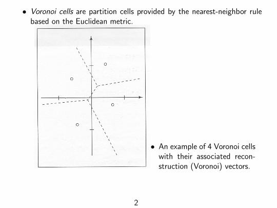
• Voronoi cells are partition cells provided by the nearest-neighbor rulebased on the Euclidean metric.

• An example of 4 Voronoi cellswith their associated recon-struction (Voronoi) vectors.

2

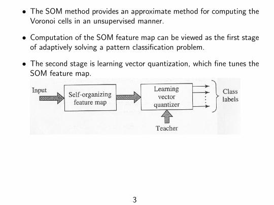
• The SOM method provides an approximate method for computing theVoronoi cells in an unsupervised manner.

• Computation of the SOM feature map can be viewed as the first stageof adaptively solving a pattern classification problem.

• The second stage is learning vector quantization, which fine tunes theSOM feature map.

3

• Learning vector quantization (LVQ) is a supervised learning technique.

• Using class information, it moves the Voronoi vectors slightly for im-proving the decision regions of the classifier.

• Take an input vector x at random from the data space.

• If the class labels of x and a Voronoi vector w agree, w is moved inthe direction of x.

• If the class labels of x and w are different, w is moved away from theinput vector x.

• Assumption: there are many more input (data) vectors x1, . . . ,xN thanVoronoi vectors w1, . . . ,wl (N � l).

4

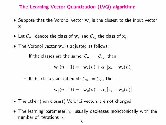
The Learning Vector Quantization (LVQ) algorithm:

• Suppose that the Voronoi vector wc is the closest to the input vectorxi.

• Let Cwc denote the class of wc and Cxithe class of xi.

• The Voronoi vector wc is adjusted as follows:

– If the classes are the same: Cwc = Cxi, then

wc(n + 1) = wc(n) + αn[xi −wc(n)]

– If the classes are different: Cwc 6= Cxi, then

wc(n + 1) = wc(n)− αn[xi −wc(n)]

• The other (non-closest) Voronoi vectors are not changed.

• The learning parameter αn usually decreases monotonically with thenumber of iterations n.

5

• For example, αn may decrease linearly from its initial value 0.1.

• The Voronoi vectors typically converge after several epochs.

6

9.8 Computer Experiment:Adaptive Pattern Classification

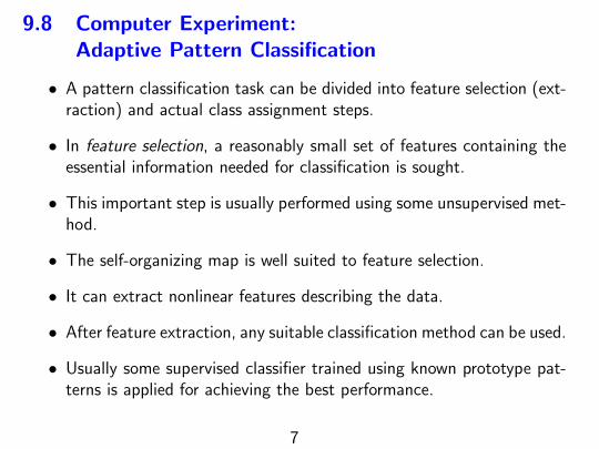
• A pattern classification task can be divided into feature selection (ext-raction) and actual class assignment steps.

• In feature selection, a reasonably small set of features containing theessential information needed for classification is sought.

• This important step is usually performed using some unsupervised met-hod.

• The self-organizing map is well suited to feature selection.

• It can extract nonlinear features describing the data.

• After feature extraction, any suitable classification method can be used.

• Usually some supervised classifier trained using known prototype pat-terns is applied for achieving the best performance.

7

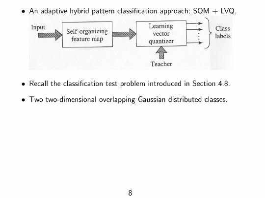
• An adaptive hybrid pattern classification approach: SOM + LVQ.

• Recall the classification test problem introduced in Section 4.8.

• Two two-dimensional overlapping Gaussian distributed classes.

8

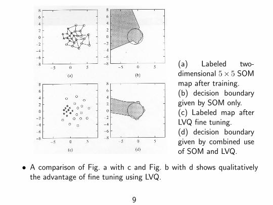
(a) Labeled two-dimensional 5×5 SOMmap after training.(b) decision boundarygiven by SOM only.(c) Labeled map afterLVQ fine tuning.(d) decision boundarygiven by combined useof SOM and LVQ.

• A comparison of Fig. a with c and Fig. b with d shows qualitativelythe advantage of fine tuning using LVQ.

9

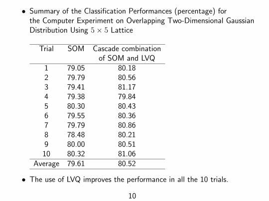
• Summary of the Classification Performances (percentage) forthe Computer Experiment on Overlapping Two-Dimensional GaussianDistribution Using 5× 5 Lattice

Trial SOM Cascade combinationof SOM and LVQ

1 79.05 80.182 79.79 80.563 79.41 81.174 79.38 79.845 80.30 80.436 79.55 80.367 79.79 80.868 78.48 80.219 80.00 80.5110 80.32 81.06

Average 79.61 80.52

• The use of LVQ improves the performance in all the 10 trials.

10

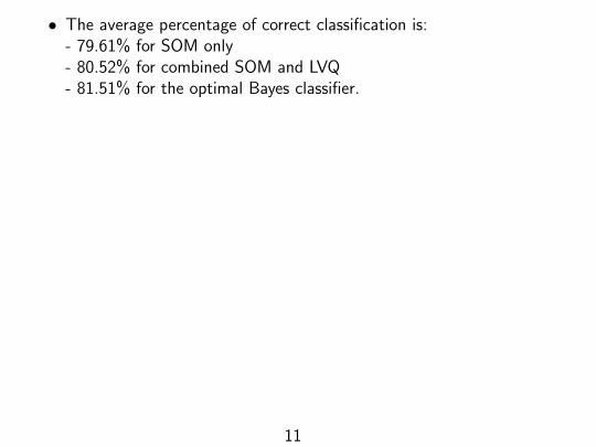
• The average percentage of correct classification is:- 79.61% for SOM only- 80.52% for combined SOM and LVQ- 81.51% for the optimal Bayes classifier.

11

9.11 Summary and Discussion

• This section describes briefly some theoretical results derived for SOM.

• Generally, it is very difficult to analyze SOM rigorously.

• The results on convergence etc. are mainly for one-dimensional latticesonly.

12