64

Chapter 4

VECTOR QUANTIZATION TECHNIQUES

4.1 INTRODUCTION

Quantization is a process of mapping an infinite set of scalar or

vector quantities by a finite set of scalar or vector quantities.

Quantization has applications in the areas of signal processing,

speech processing and Image processing. In speech coding,

quantization is required to reduce the number of bits used to

represent a sample of speech signal. When less number of bits is used

to represent a sample the bit-rate, complexity and memory

requirement gets reduced. Quantization results in the loss in the

quality of a speech signal, which is undesirable. So a compromise

must be made between the reduction in bit-rate and the quality of

speech signal.

Two types of quantization techniques exist. They are scalar

quantization and vector quantization. “Scalar quantization deals with

the quantization of samples on a sample by sample basis”, while

“vector quantization deals with quantizing the samples in groups

called vectors”. Vector quantization increases the optimality of a

quantizer at the cost of increased computational complexity and

memory requirements.

Shannon theory states that “quantizing a vector is more effective

than quantizing individual scalar values in terms of spectral

distortion”. According to Shannon the dimension of a vector chosen

65

greatly affects the performance of quantization. Vectors of larger

dimension produce better quality compared to vectors of smaller

dimension and in vectors of smaller dimension the transparency in

the quantization is not good at a particular bit-rate chosen [8]. This is

because in vectors of smaller dimension the correlation that exists

between the samples is lost and the scalar quantization itself destroys

the correlation that exists between successive samples. So the quality

of the quantized speech signal gets lost. Therefore, quantizing

correlated data requires techniques that preserve the correlation

between the samples, which is achieved by the vector quantization

technique (VQ). Vector quantization is the simplification of scalar

quantization. Vectors of larger dimension produce transparency in

quantization at a particular bit-rate chosen. In Vector quantization the

data is quantized in the form of contiguous blocks called vectors

rather than individual samples. But later with the development of

better coding techniques, it is made possible that transparency in

quantization can also be achieved even for vectors of smaller

dimension. In this thesis quantization is performed on vectors of full

length and on vectors of smaller dimensions for a given bit-rate [4,

50].

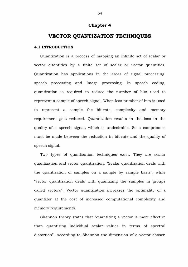
An example of two dimensional vector quantizer is shown in Fig

4.1. The two dimensional region shown in Fig 4.1 is called as the

voronoi region, which in turn contains several numbers of small

hexagonal regions. The hexagonal regions defined by the red borders

are called as the encoding regions. The green dots represent the

66

vectors to be quantized which fall in different hexagonal regions and

the blue circles represent the codeword‟s (centroids). The vectors

(green dots) falling in a particular hexagonal region is best represented

by the codeword (blue circle) falling in that hexagonal region [51-54].

Fig 4.1 Two Dimensional Vector Quantizer

Vector quantization technique has become a great tool with the

development of non variational design algorithms like the Linde, Buzo,

Gray (LBG) algorithm. On the other hand besides spectral distortion

the vector quantizer is having its own limitations like the

computational complexity and memory requirements required for the

searching and storing of the codebooks. For applications requiring

higher bit-rates the computational complexity and memory

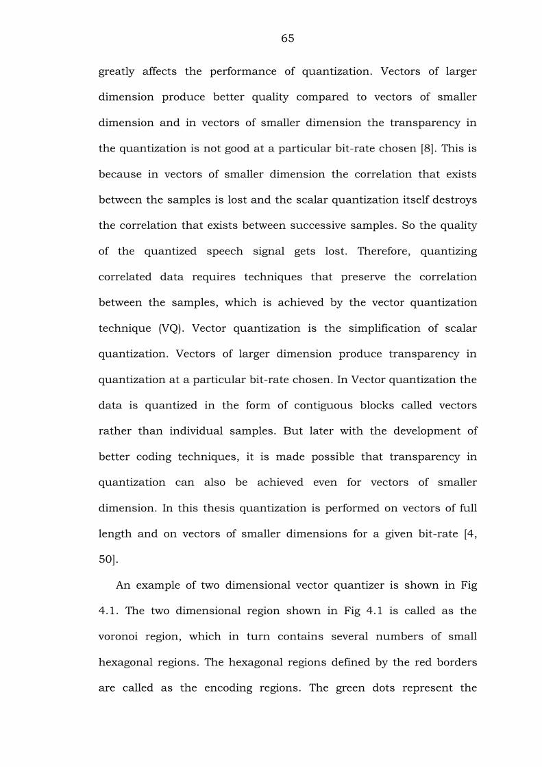
requirements increases exponentially. The block diagram of a vector

quantizer is shown in Fig 4.2.

67

Fig 4.2 Block diagram of Vector Quantizer

Let T

N1 2ks s , s ,......, s

be an „ N ‟ dimensional vector with real

valued samples in the range 1 k N . The superscript „T ‟ in the

vector k

s denotes the transpose of the vector. In vector quantization, a

real valued „N‟ dimensional input vector k

s is matched with the real

valued „ N ‟ dimensional codewords of the codebook bN 2 . The

codeword that best matches the input vector with lowest distortion is

taken and the input vector is replaced by it. The codebook consists of

a finite set of codewords C = iC , 1 i  L , where

T

i i 1 i 2 i NC C , C ,......., C , where „C ‟ is the codebook, „ L ‟ is the length of

the codebook and iC denote the ith codeword in a codebook. In Fig 4.2

ns represents the line spectral frequencies (LSF) to be quantized. In

this work the number of line spectral frequencies per frame is ten and

they are extracted from the eleven linear predictive coefficients of a

frame using the matlab command poly2lsf.

Index i

Input Vector

Buffer

Codebook with

Codeword’s

C

Vector

Quantizer

ns ks

iC

68

4.2 LINE SPECTRAL FREQUENCIES

The parameters used in the analysis and synthesis of the speech

signals are the LPC coefficients. In speech coding the quantization is

not performed directly on the LPC coefficients, but the quantization is

performed by transforming the LPC coefficients to other forms which

ensure filter stability after quantization. Another reason for not using

LPC coefficients is that LPC coefficients have a wide dynamic range

and so the LPC filter easily becomes unstable after quantization. So

LPC coefficients are not used for quantization. The alternative to LPC

coefficients is the use of line spectral frequency (LSF) parameters

which ensure filter stability after quantization. The filter stability is

checked easily just by observing the order of the LSF samples in an

LSF vector after quantization. If the LSF samples in a vector are in the

ascending or descending order the filter stability is ensured otherwise

the filter stability cannot be ensured [54-58].

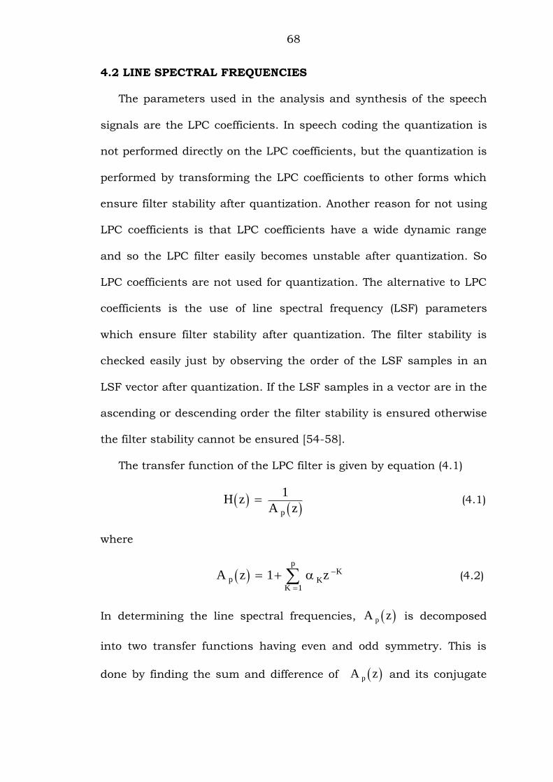
The transfer function of the LPC filter is given by equation (4.1)

p

1H z

A z (4.1)

where

p

K p K

K 1

A z 1 z

(4.2)

In determining the line spectral frequencies, pA z is decomposed

into two transfer functions having even and odd symmetry. This is

done by finding the sum and difference of pA z and its conjugate

69

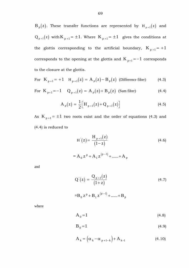
pB z . These transfer functions are represented by p 1H z and

p 1Q z with p 1K 1 . Where p 1K 1 gives the conditions at

the glottis corresponding to the artificial boundary, p 1K 1

corresponds to the opening at the glottis and p 1K 1 corresponds

to the closure at the glottis.

For p 1K 1 p p p 1H z A z  B z (Difference filter) (4.3)

For p 1K 1 p p p 1Q z A z  B z (Sum filter) (4.4)

p p 1 p 1

1A z H z Q z

2

(4.5)

As p 1K 1 two roots exist and the order of equations (4.3) and

(4.4) is reduced to

p 1'H

H zz

1 z

(4.6)

p 1 p p0 1= A z A z ...... A

and

p 1'

Q zQ z

1 z

(4.7)

p 1pp0 1=B z B z ...... B

where

0A 1 (4.8)

0B 1 (4.9)

k k p 1 k k -1A A

(4.10)

70

k k p 1 k k - 1B - B

(4.11)

for k = 1 ,…….., p

The angular positions of the roots of 'H z and 'Q z gives us the

line spectral frequencies and occurs in complex conjugate pairs. The

line spectral frequencies range fromi

.

The line spectral frequencies have the following properties:

All the roots of 'H z and 'Q z must lie on the unit circle

which is the required condition for stability.

The roots of 'H z and 'Q z are arranged in an alternate

manner on the unit circle i.e., q , 0 p ,0 q ,1 p ,1 ........., .

The roots of equation (4.6) is obtained using the real root method [31]

and is explained in the following section.

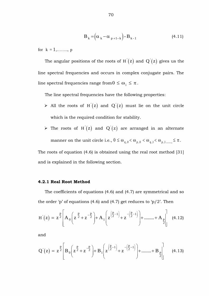
4.2.1 Real Root Method

The coefficients of equations (4.6) and (4.7) are symmetrical and so

the order „p‟ of equations (4.6) and (4.7) get reduces to „p/2‟. Then

p pp p p 1 12 2' 2 2 2

p0 12

H z z A z z A z z ........ A

(4.12)

and

p pp p p 1 12 2' 2 2 2

p0 12

Q z z B z z B z z ........ B

(4.13)

71

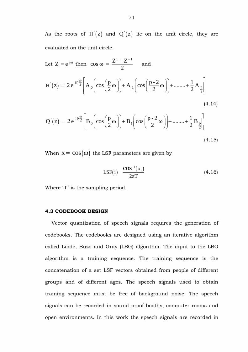
As the roots of 'H z and 'Q z lie on the unit circle, they are

evaluated on the unit circle.

Let  jZ e then 1 1Z Z

cos 2

and

 jp' 2

p0 12

Hp p - 2 1

z 2 e A cos A cos ........ A2 2 2

(4.14)

 jp' 2

p0 12

p p - 2 1Q z 2 e B cos B cos ........ B

2 2 2

(4.15)

When x cos the LSF parameters are given by

1

ixLSF i

2 T

cos

(4.16)

Where „ T ‟ is the sampling period.

4.3 CODEBOOK DESIGN

Vector quantization of speech signals requires the generation of

codebooks. The codebooks are designed using an iterative algorithm

called Linde, Buzo and Gray (LBG) algorithm. The input to the LBG

algorithm is a training sequence. The training sequence is the

concatenation of a set LSF vectors obtained from people of different

groups and of different ages. The speech signals used to obtain

training sequence must be free of background noise. The speech

signals can be recorded in sound proof booths, computer rooms and

open environments. In this work the speech signals are recorded in

72

computer rooms. In practice speech data base like TIMIT database is

available for use in speech coding and speech recognition.

The codebook generation using LBG algorithm requires the

generation of an initial codebook, which is the centroid or mean

obtained from the training sequence. The centroid obtained is then

split into two centroids or codewords using the splitting method. The

iterative LBG algorithm splits these two codeword‟s into four, four into

eight and the process continues till the required numbers of

codewords in the codebook are obtained [59-61].

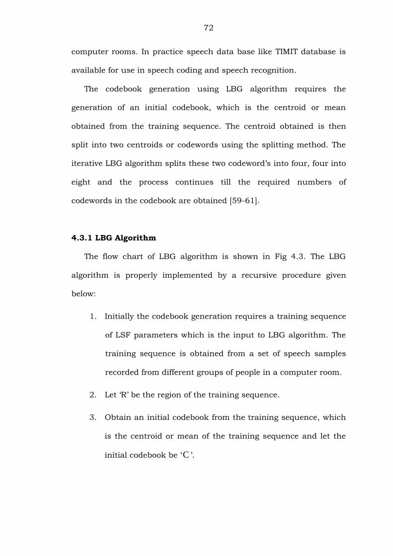
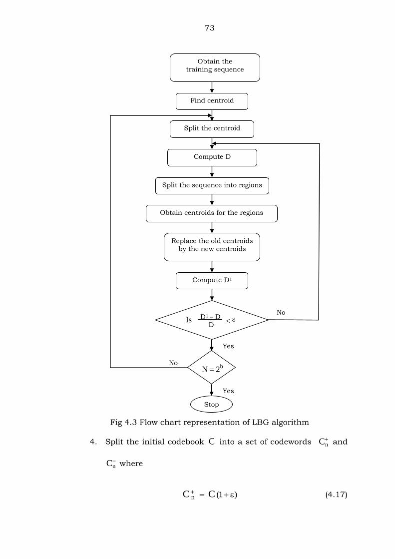
4.3.1 LBG Algorithm

The flow chart of LBG algorithm is shown in Fig 4.3. The LBG

algorithm is properly implemented by a recursive procedure given

below:

1. Initially the codebook generation requires a training sequence

of LSF parameters which is the input to LBG algorithm. The

training sequence is obtained from a set of speech samples

recorded from different groups of people in a computer room.

2. Let „R‟ be the region of the training sequence.

3. Obtain an initial codebook from the training sequence, which

is the centroid or mean of the training sequence and let the

initial codebook be „C ‟.

73

Fig 4.3 Flow chart representation of LBG algorithm

4. Split the initial codebook C into a set of codewords nC and

nC where

n (1 )C C (4.17)

Obtain the

training sequence

Find centroid

Split the centroid

Compute D

Split the sequence into regions

Obtain centroids for the regions

Replace the old centroids

by the new centroids

Compute D1

Is <

bN 2

Stop

Yes

No

No

Yes

D1 – D

D

74

n (1 )C C (4.18)

0.01 is the minimum error to be obtained between old and

new codewords.

5. Compute the difference between the training sequence and

each of the codeword‟s nC and nC and let the difference be

„D‟.

6. Split the training sequence into two regions R1 and R2

depending on the difference „D‟ between the training sequence

and the codeword‟s nC and nC . The training vectors closer to

nC falls in the region R1 and the training vectors closer to nC

falls in the region R2.

7. Let the training vectors falling in the region R1 be TV1 and the

training sequence vectors falling in the region R2 be TV2.

8. Obtain the new centroid or mean for TV1 and TV2. Let the new

centroids be CR1 and CR2.

9. Replace the old centroids nC and nC by the new centroids

CR1 and CR2.

10. Compute the difference between the training sequence and

the new centroids CR1 and CR2 and let the difference be 1D .

11. Repeat steps 5 to 10 until 1D – D

D .

12. Repeat steps 4 to 11 till the required number of codewords in

the codebook are obtained.

75

where bN 2 represents the number of codewords in the codebook

and „ b ‟ represents the number of bits used for codebook generation,

„ D ‟ represents the difference between the training sequence and the

old codewords and 1D represents the difference between the training

sequence and the new codewords.

4.4 SPECTRAL DISTORTION

The quality of the speech signal is an important parameter in

speech coders and is measured in terms of spectral distortion

measured in decibels (dB). The spectral distortion is measured

between the LPC power spectra of the quantized and unquantized

speech signals. The spectral distortion is measured frame wise and

the average or mean of the spectral distortion calculated over all

frames is taken as the final value of the spectral distortion. For a

quantizer to be transparent the mean of the spectral distortion must

be less than 1 dB without any audible distortion in the reconstructed

speech. But the mean of the spectral distortion is not a sufficient

measure to find the performance of a quantizer, this is because the

human ear is sensitive to large quantization errors that occur

occasionally. So in addition to measuring the mean of the spectral

distortion it is also necessary to have another measure of quality

which is the percentage number of frames having a spectral distortion

greater than 2dB and less than 4dB and the percentage number of

frames having a spectral distortion greater than 4dB. The frames

76

having spectral distortion between 2 to 4dB and greater than 4dB are

called as outlier frames [54].

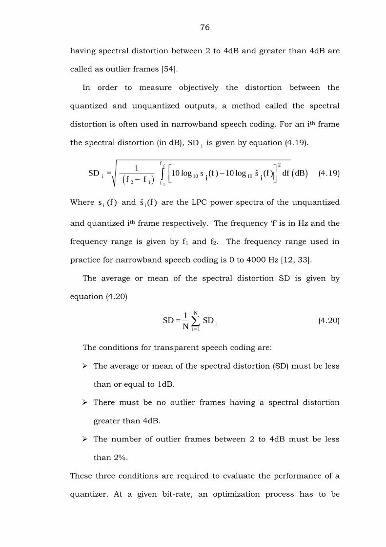
In order to measure objectively the distortion between the

quantized and unquantized outputs, a method called the spectral

distortion is often used in narrowband speech coding. For an ith frame

the spectral distortion (in dB), iSD is given by equation (4.19).

2

1

f 2

10 10i

2 1 f

ˆs si i

1SD = 10 log (f ) 10 log (f ) df dB

f f

(4.19)

Where is (f ) and is (f ) are the LPC power spectra of the unquantized

and quantized ith frame respectively. The frequency „f‟ is in Hz and the

frequency range is given by f1 and f2. The frequency range used in

practice for narrowband speech coding is 0 to 4000 Hz [12, 33].

The average or mean of the spectral distortion SD is given by

equation (4.20)

N

ii =1

1SD = SD

N (4.20)

The conditions for transparent speech coding are:

The average or mean of the spectral distortion (SD) must be less

than or equal to 1dB.

There must be no outlier frames having a spectral distortion

greater than 4dB.

The number of outlier frames between 2 to 4dB must be less

than 2%.

These three conditions are required to evaluate the performance of a

quantizer. At a given bit-rate, an optimization process has to be

77

carried out so as to obtain better performance i.e., accepting a large

average spectral distortion for a few outliers.

4.5 WEIGHTED LSF DISTANCE MEASUREMENT

In the design of a vector quantizer instead of using the mean

squared error (MSE) distance measure the weighted LSF distance

measurement is used. This is done to place emphasis on the low

frequency LSFs and on the LSFs with higher power spectrum. The

weights used are of two types. They are static or dynamic [54].

Fixed or Static weights iS : These are used to place emphasis

on the low frequency LSFs in order to account for the sensitivity

of human ear for low and high frequency LSFs.

Varying or Dynamic weights iW : These are used to place

emphasis on the LSFs with high power spectrum.

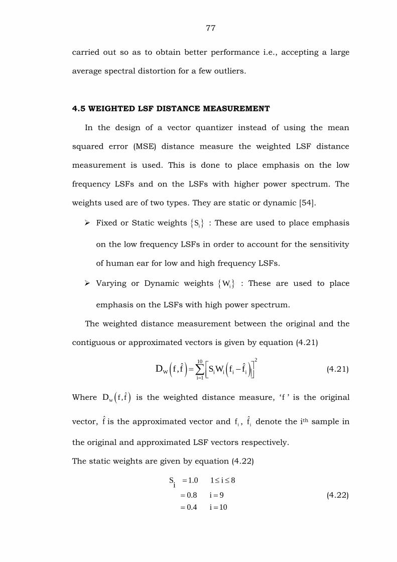
The weighted distance measurement between the original and the

contiguous or approximated vectors is given by equation (4.21)

210

W i i i ii 1

ˆ ˆf ,f S W f fD

(4.21)

Where Wˆf , fD is the weighted distance measure, „ f ‟ is the original

vector, f is the approximated vector and if , if denote the ith sample in

the original and approximated LSF vectors respectively.

The static weights are given by equation (4.22)

S 1.0 1 i 8i

0.8 i 9

0.4 i 10

(4.22)

78

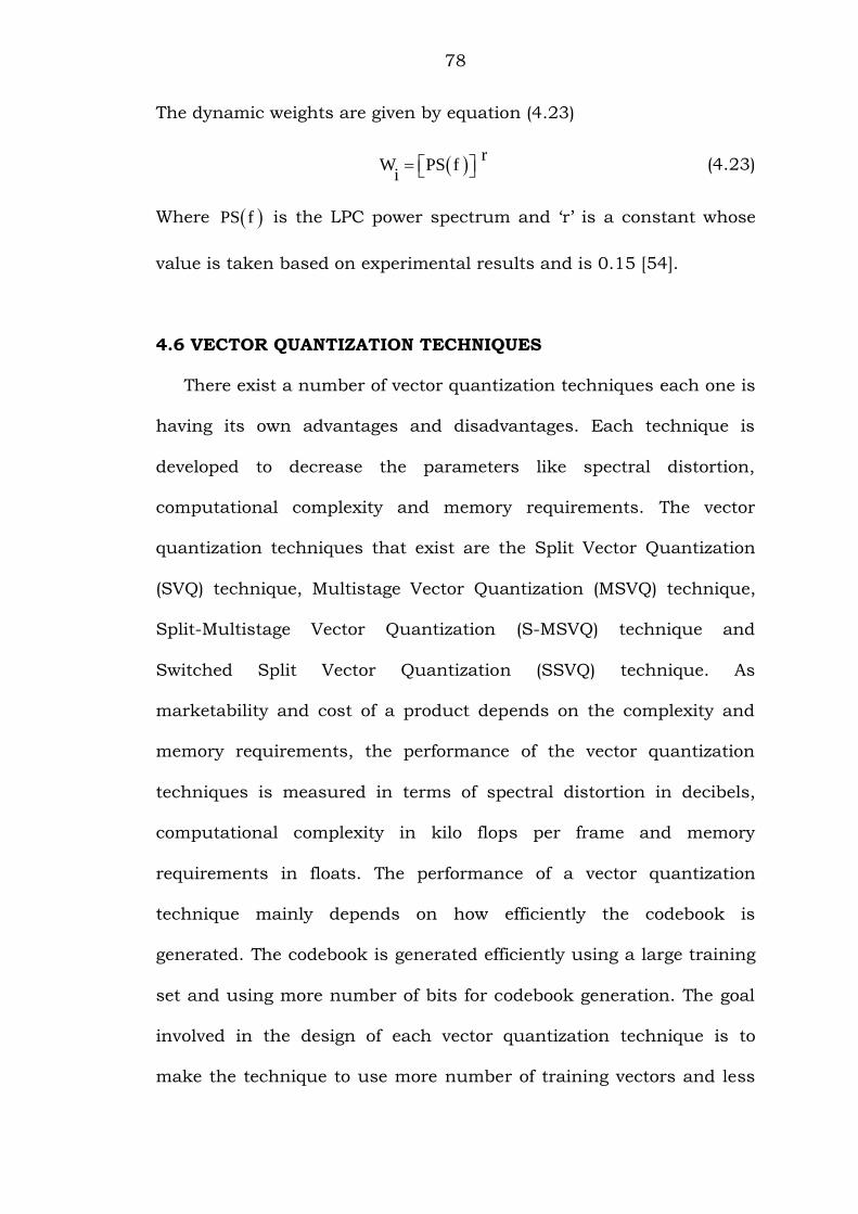
The dynamic weights are given by equation (4.23)

r

W PS fi (4.23)

Where PS f is the LPC power spectrum and „r‟ is a constant whose

value is taken based on experimental results and is 0.15 [54].

4.6 VECTOR QUANTIZATION TECHNIQUES

There exist a number of vector quantization techniques each one is

having its own advantages and disadvantages. Each technique is

developed to decrease the parameters like spectral distortion,

computational complexity and memory requirements. The vector

quantization techniques that exist are the Split Vector Quantization

(SVQ) technique, Multistage Vector Quantization (MSVQ) technique,

Split-Multistage Vector Quantization (S-MSVQ) technique and

Switched Split Vector Quantization (SSVQ) technique. As

marketability and cost of a product depends on the complexity and

memory requirements, the performance of the vector quantization

techniques is measured in terms of spectral distortion in decibels,

computational complexity in kilo flops per frame and memory

requirements in floats. The performance of a vector quantization

technique mainly depends on how efficiently the codebook is

generated. The codebook is generated efficiently using a large training

set and using more number of bits for codebook generation. The goal

involved in the design of each vector quantization technique is to

make the technique to use more number of training vectors and less

79

number of bits for codebook generation, there by the spectral

distortion, computational complexity and memory requirements get

reduced. It has been observed that as the number of bits used for

codebook generation decreases the computational complexity and

memory requirements decreases but the spectral distortion increases.

This increase in spectral distortion is reduced by increasing the

number of training vectors used for codebook generation [62-71].

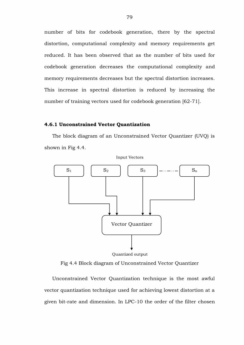
4.6.1 Unconstrained Vector Quantization

The block diagram of an Unconstrained Vector Quantizer (UVQ) is

shown in Fig 4.4.

Fig 4.4 Block diagram of Unconstrained Vector Quantizer

Unconstrained Vector Quantization technique is the most awful

vector quantization technique used for achieving lowest distortion at a

given bit-rate and dimension. In LPC-10 the order of the filter chosen

S1 S2

S3

Sn

Vector Quantizer

Input Vectors

Quantized output

80

is 10 and so the length of each LSF vector is 10. In Unconstrained

Vector Quantization technique the quantization is done on vectors of

full length i.e., vectors containing all the ten line spectral frequencies.

In Fig 4.4 S1, S2, S3……Sn are the input LSF vectors to be quantized

using the Unconstrained Vector Quantizer.

The main advantage of UVQ is that it is expected to give lowest

spectral distortion for a given bit-rate as the correlation that exists

between the samples of a vector is preserved. But the disadvantage of

UVQ is that as vectors of full length are used, at higher bit-rates the

complexity and memory requirements increases in an exponential

manner making it impractical for applications requiring higher bit-

rates. Another problem with UVQ is that the generation of codebook

becomes a difficult task on general purpose computers as the memory

available with them is limited. So the number of training vectors used

for codebook generation must be limited in number or the length of

each vector must be reduced. In practice on general purpose

computers, using UVQ technique the generation of codebook at higher

bit-rates is a difficult task, even though the training data contains less

number of training vectors. But the number of training vectors

required to generate the codebook must be large than the number of

codewords in a codebook otherwise there will be too much over fitting

of the training set [54].

The computational complexity and memory requirements of a „ b ‟

bit, „ n ‟ dimensional vector quantizer are calculated as follows [54]:

81

To calculate the mean square error (MSE) between two vectors

of „ n ‟ dimension, „ n ‟ subtractions, „ n ‟ multiplications and 1n

additions are required. So a total of 3n 1 flops are required.

To search a codebook of b2 code vectors, b3n 1 2 flops are

required in addition to the minimum distortion search requiring

b2 1 flops.

So the number of computations made by a „ b ‟ bit, „ n ‟

dimensional vector quantizer is

b bTotal complexity 3n 1 2 2 1

b 3n2 1 flops per vector. (4.24)

In computing the complexity each addition, multiplication and

comparison is considered as one floating point operation. So a „ b ‟ bit

„ n ‟ dimensional vector quantizer requires a codebook of b2 code

words, needs to store bn2 floating point values and computes b3n 1 2

flops per vector. In the design of a vector quantizer if weighted

distance measure is used instead of mean square error distance

measure the complexity increases from b3n 1 2 to b4n2 1 flops per

vector.

The computational complexity of an Unconstrained Vector

Quantizer is given by equation (4.25)

b

UVQComplexity 4n2 1 flops/frame (4.25)

where

n is the dimension of the vector

82

b is the number of bits allocated to the vector quantizer.

The memory requirement of an Unconstrained Vector Quantizer is

given by equation (4.26)

b 

UVQMemory n2 floats (4.26)

4.6.2 Product Code Vector Quantization

Exhaustive search vector quantizers achieve lowest distortion at

the expense of complexity and memory requirements at higher bit-

rates. So to make the vector quantizers more practical for vectors of

larger dimension and higher bit-rates structural constraints are

imposed on the design of a vector quantizer or codebook. One way of

achieving this is by decomposing the codebook into a Cartesian

product of smaller codebooks i.e., m1 2 3C C * C * C . ..* C . The

advantage with smaller codebooks is that the computational

complexity and memory requirements are reduced to a very great

extent. This is because the number of bits used for codebook

generation is divided among the sets of the decomposed codebook [12,

18]. Examples of product code vector quantization techniques are

Split Vector Quantization (SVQ), Multistage Vector Quantization

(MSVQ), Split-Multistage Vector Quantization (S-MSVQ), Switched

Split Vector Quantization (SSVQ). In this thesis two product code

vector quantization techniques are proposed. They are: Switched

Multistage Vector Quantization (SWMSVQ) and Multi Switched Split

Vector Quantization (MSSVQ) techniques [54, 72].

83

4.6.2.1 Split Vector Quantization

The main disadvantage of Unconstrained Vector Quantizer is high

complexity, memory requirements and the generation of codebook is a

difficult task as vectors of full length are used for quantization without

any structural constraint. As a result more number of training vectors

and bits cannot be used for codebook generation. With these

constraints the quantizer cannot produce better quality quantized

outputs. So to improve the performance of Unconstrained Vector

Quantization technique a well known technique called Split Vector

Quantization has been developed. The concept behind Split Vector

Quantization is that the vectors of larger dimensions are split into

vectors of smaller dimensions and the bits allocated to the quantizer

are divided among the splits (parts). Due to splitting, the dimension of

a vector gets decreased hence more number of training vectors and

bits are used for codebook generation. As a result the performance of

quantization is increased, the complexity and memory requirements

are reduced. But the main disadvantage with this technique is that,

due to splitting the linear and non linear dependencies that exist

between the samples of a vector is lost and the shape of the quantizer

cells is affected. As a result the spectral distortion increases slightly.

This increase in spectral distortion is compensated by increasing the

number of training vectors and using more number of bits for

codebook generation. The number of splits in this type of quantizer

must be limited in number otherwise the vector quantizer will act as a

scalar quantizer.

84

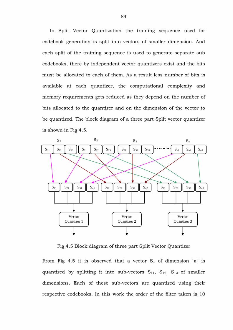
In Split Vector Quantization the training sequence used for

codebook generation is split into vectors of smaller dimension. And

each split of the training sequence is used to generate separate sub

codebooks, there by independent vector quantizers exist and the bits

must be allocated to each of them. As a result less number of bits is

available at each quantizer, the computational complexity and

memory requirements gets reduced as they depend on the number of

bits allocated to the quantizer and on the dimension of the vector to

be quantized. The block diagram of a three part Split vector quantizer

is shown in Fig 4.5.

Fig 4.5 Block diagram of three part Split Vector Quantizer

From Fig 4.5 it is observed that a vector S1 of dimension „ n ‟ is

quantized by splitting it into sub-vectors S11, S12, S13 of smaller

dimensions. Each of these sub-vectors are quantized using their

respective codebooks. In this work the order of the filter taken is 10

S12 S22 Sn2 S32 S11 S21 Sn1 S31 S13 S23 Sn3 S33

Vector

Quantizer 1

Vector

Quantizer 2

Vector

Quantizer 3

S21 S22 S23 S31 S32 S33 Sn1 Sn2 Sn3 S11 S12 S13

S1 S2 S3 Sn

85

and so the LSF vector contain 10 samples and these 10 samples are

split into three parts of 3, 3, 4 samples [54, 73-75].

From results of Split Vector Quantization technique it is proved

that the computational complexity and memory requirements gets

decreased compared to Unconstrained Vector Quantization technique.

So Split Vector Quantization technique is proved to be superior to

Unconstrained Vector Quantization technique in terms of the

computational complexity and memory requirements.

In an „ n ‟ dimensional Split Vector Quantizer of „sp ‟ splits and „b ‟

bits per vector. The vector space Rn is split into „sp ‟ subspaces or

splits or parts of lower dimension, then the dimension of a subspace is

ni where

spn n

ii 1

. The number of independent quantizers is equal to

the number of splits and the bits used for quantization are divided

among the splits. When bi is the bits allocated to each split of the

vector quantizer then the total bits allocated to the quantizer is

spb b

ii 1

[54].

The computational complexity of a Split Vector Quantizer is given

by equation (4.27)

sp biComplexity 4n 2 1

SVQ ii 1

(4.27)

86

where

in is the dimension of a sub-vector in ith split

ib is the number of bits allocated to the ith split of a quantizer

sp is the number of splits.

The Memory requirements of a Split Vector Quantizer is given by

equation (4.28)

sp biMemory n 2

SVQ ii 1

(4.28)

4.6.2.2 Multistage Vector Quantization

Multistage Vector Quantization is a modification of Unconstrained

Vector Quantization technique. It is also called as Multistep, Residual

or Cascaded Vector Quantization. Multistage Vector Quantization

(MSVQ) technique preserves all the features of Unconstrained Vector

Quantization technique while decreasing the computational

complexity, memory requirements and spectral distortion. Multistage

Vector Quantization technique shows significant improvement in the

quality of the speech signal by decreasing the spectral distortion, but

the computational complexity and memory requirements are high

compared to Split Vector Quantization technique. This is because

Split Vector Quantization technique deals with the vectors of lower

dimensions while Unconstrained and Multistage Vector Quantization

techniques deal with vectors of larger dimensions.

87

Multistage Vector Quantizer is a cascaded connection of several

vector quantizers, where the output of one stage is given as an input

to the next stage and the bits used for quantization are divided among

the stages connected in cascade [12, 14]. As a result less number of

bits are available at each stage due to which the computational

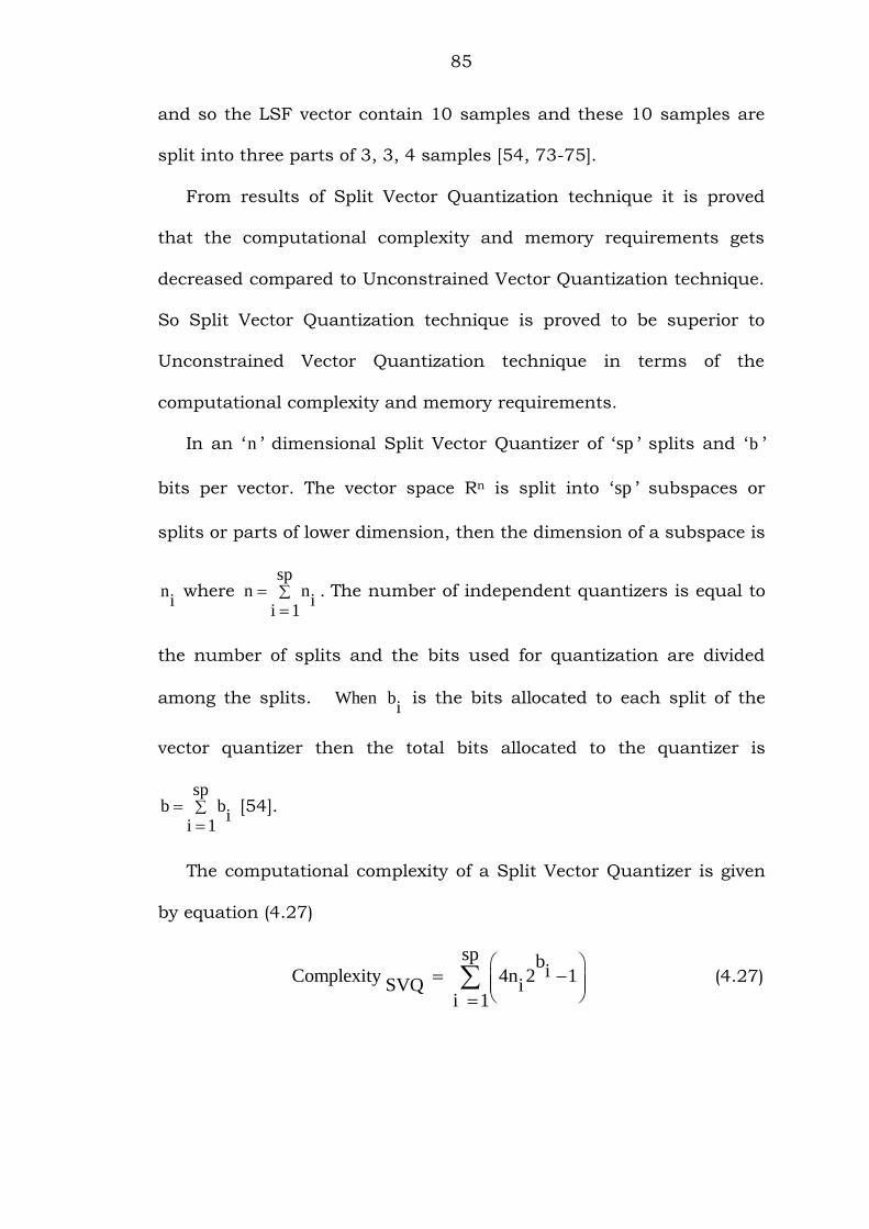
complexity and memory requirements get reduced. The generation of

codebooks at different stages of a three stage MSVQ is shown in Fig

4.6.

Fig 4.6 Generation of codebooks at different stages of Multistage

Vector Quantizer

From Fig 4.6 it is observed that the codebook at the first stage is

generated by taking the training sequence as an input. At the second

stage the codebook is generated using the quantization errors of the

first stage, likewise the codebook at the third stage is generated using

2nd Stage Codebook

LBG Algorithm

2nd Stage

Training Sequence

1st Stage

Codebook

Vector Quantizer

1st Stage

Training Sequence

Training

Sequence

LBG Algorithm

88

the quantization errors of the second stage. This process is continued

for the required number of stages [76-80].

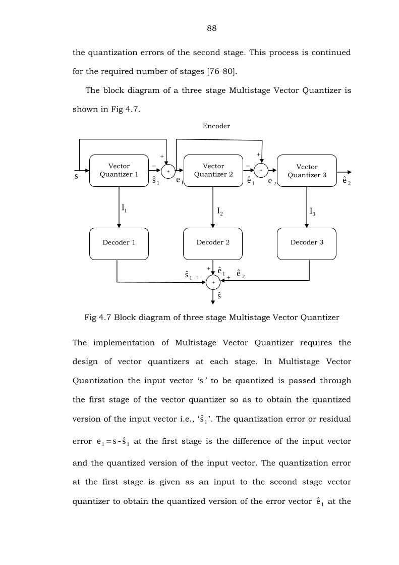
The block diagram of a three stage Multistage Vector Quantizer is

shown in Fig 4.7.

Fig 4.7 Block diagram of three stage Multistage Vector Quantizer

The implementation of Multistage Vector Quantizer requires the

design of vector quantizers at each stage. In Multistage Vector

Quantization the input vector „s ‟ to be quantized is passed through

the first stage of the vector quantizer so as to obtain the quantized

version of the input vector i.e., „ 1s ’. The quantization error or residual

error 1 1ˆe s - s at the first stage is the difference of the input vector

and the quantized version of the input vector. The quantization error

at the first stage is given as an input to the second stage vector

quantizer to obtain the quantized version of the error vector 1e at the

1s +

+

+

+

_

_

+

Vector

Quantizer 1 s

1I

Encoder

1s

3I 2I

Decoder 1

Decoder 2

Decoder 3

+

Vector

Quantizer 2

Vector

Quantizer 3 +

1e

1e 2e

+

s

1e 2e

2e

89

first stage. Likewise the quantization error at the second stage

2 1 1ˆe e - e

is given as input to the third stage vector quantizer to

obtain the quantized version of the error vector at the second stage

i.e., 2e and this process continues for the required number of stages.

Finally the decoder takes the indices Ii from each quantizer stage and

adds the corresponding codewords to obtain the quantized version of

the input vector i.e., 1 1 2ˆ ˆ ˆ ˆs s e e [54].

In a Multistage Vector Quantizer each stage acts as an

independent vector quantizer and the total bits available for vector

quantization are divided among the stages. Then the complexity of a

stage equals the complexity of Unconstrained Vector Quantizer and is

jb

4n2 1 , where jb is the number of bits allocated to the jth stage.

Likewise the memory requirements of a stage in Multistage Vector

Quantizer is jb

n2 .

The computational complexity of a Multistage Vector Quantizer is

given by equation (4.29)

p bj

Complexity 4n2 1MSVQ

j 1

(4.29)

where

n is the dimension of the vector

jb is the number of bits allocated to the jth stage

P is the number of stages

90

The Memory requirements of a Multistage Vector Quantizer is given

by equation (4.30)

MSVQ

bp jMemory n2

j 1

(4.30)

4.6.2.3 Split-Multistage Vector Quantization

In order to improve the performance of Multistage Vector

Quantization and Split Vector Quantization techniques a hybrid

product code vector quantization technique, called Split-Multistage

Vector Quantization (S-MSVQ) technique is developed. Split-

Multistage Vector Quantization technique is a hybrid of Split Vector

Quantization and Multistage Vector Quantization techniques. Split-

Multistage Vector Quantization technique offer lowest spectral

distortion, complexity and memory requirements than the

Unconstrained Vector Quantization, Multistage Vector Quantization

and Split Vector Quantization techniques [73-80]. The decrease in

spectral distortion is due to summing of the quantized errors at each

stage.

In Split-Multistage Vector Quantization the dimension of vectors

to be quantized is reduced by means of splitting and the bits allocated

to the quantizer are divided among the stages and splits of each stage.

As a result the dimension of the vectors to be quantized and the bits

at each stage & split are reduced which decreases the complexity and

memory requirements compared to Unconstrained Vector

Quantization, Multistage Vector Quantization and Split Vector

Quantization techniques.

91

The generation of the codebooks at each stage of the Split-

Multistage Vector Quantizer is similar to the codebooks generation at

each stage of the Multistage Vector Quantizer. But the difference is

that each stage of the Split-Multistage Vector Quantizer involves the

generation of several sub codebooks. The number of sub codebooks

generated at each stage is equal to the number of splits at that stage.

In this work, Split-Multistage Vector Quantizer with three parts (splits)

and three stages have been developed. The performance of

quantization depends on the number of stages and on the number of

splits at each stage. As the number of stages increases the quality of

the quantized output is increased, but there must be a limit on the

number of stages and on the number of splits at each stage as the

number of bits at each stage is limited.

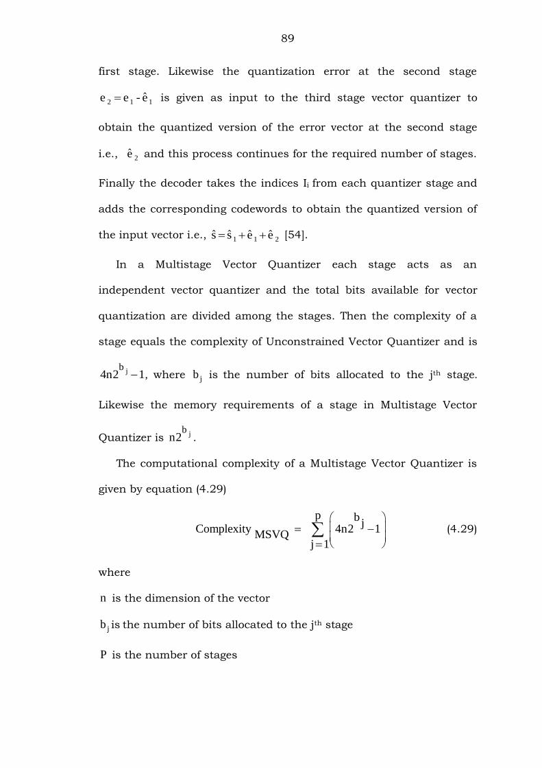
The allocation of the bits to a stage is shown in Table 4.1.

Table 4.1 Allocation of bits to a stage

Number of bits

/ frame

Number of

stages

Bits allocation

at each stage

24 3 8,8,8

23 3 8,8,7

22 3 8,7,7

9 3 3,3,3

8 3 3,3,2

92

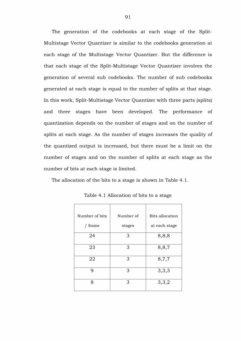
The allocation of the bits at each split of a stage is shown in Table 4.2.

Table 4.2 Allocation of bits to each split of a stage

Number of bits

at each stage

Number of

splits / stage

Bits allocation

to each split

8 3 2,3,3

7 3 2,2,3

6 3 2,2,2

3 3 1,1,1

2 3 0,1,1

From Tables 4.1 and 4.2 it is observed that the minimum number

of bits at each stage with three parts must be at least three. So with

three parts (splits) and three stages, in Split-Multistage Vector

Quantizer the number of bits at a frame cannot be reduced below 9

bits.

The block diagram of a Split-Multistage Vector Quantizer with

three parts and three stages is shown in Fig 4.8. The block diagram is

similar to three stage Multistage Vector Quantizer except for the splits

at each stage. In Split-Multistage Vector Quantizer each split is

treated as a separate vector quantizer and the vectors at each split are

quantized independently. The quantization mechanism involved in

Split-Multistage Vector Quantizer is similar to the quantization

process involved in Multistage Vector Quantizer, except that in Split-

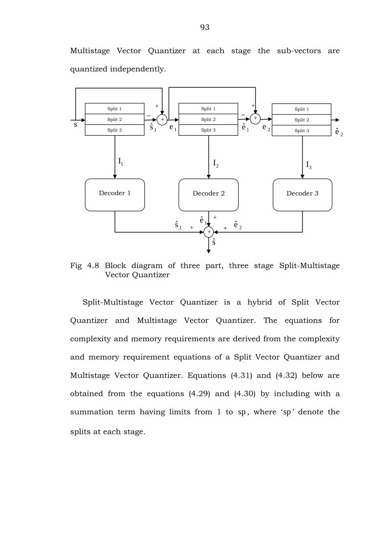
93

Multistage Vector Quantizer at each stage the sub-vectors are

quantized independently.

Fig 4.8 Block diagram of three part, three stage Split-Multistage

Vector Quantizer

Split-Multistage Vector Quantizer is a hybrid of Split Vector

Quantizer and Multistage Vector Quantizer. The equations for

complexity and memory requirements are derived from the complexity

and memory requirement equations of a Split Vector Quantizer and

Multistage Vector Quantizer. Equations (4.31) and (4.32) below are

obtained from the equations (4.29) and (4.30) by including with a

summation term having limits from 1 to sp , where „sp ‟ denote the

splits at each stage.

1s 1e

s

2e +

+

+

Decoder 1

Decoder 2

Decoder 3

3I 2I 1I

2e

Split 1

Split 2

Split 3

2e 1e

_

+ Split 1

Split 2

Split 3

Split 1

Split 2

Split 3

1e 1s

_

+

s

+

+

+

94

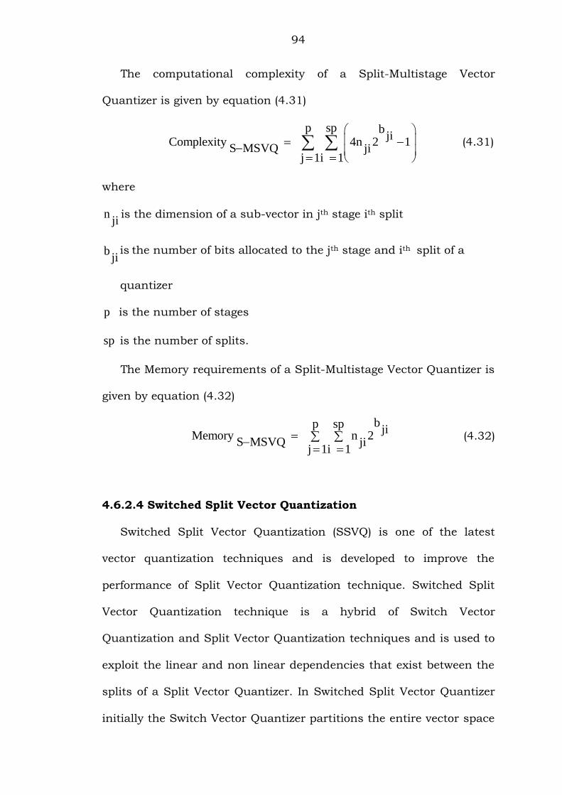
The computational complexity of a Split-Multistage Vector

Quantizer is given by equation (4.31)

p sp bji

Complexity 4n 2 1S MSVQ ji

j 1i 1

(4.31)

where

nji

is the dimension of a sub-vector in jth stage ith split

bji

is the number of bits allocated to the jth stage and ith split of a

quantizer

p is the number of stages

sp is the number of splits.

The Memory requirements of a Split-Multistage Vector Quantizer is

given by equation (4.32)

bp sp jiMemory n 2

S MSVQ ji j 1i 1

(4.32)

4.6.2.4 Switched Split Vector Quantization

Switched Split Vector Quantization (SSVQ) is one of the latest

vector quantization techniques and is developed to improve the

performance of Split Vector Quantization technique. Switched Split

Vector Quantization technique is a hybrid of Switch Vector

Quantization and Split Vector Quantization techniques and is used to

exploit the linear and non linear dependencies that exist between the

splits of a Split Vector Quantizer. In Switched Split Vector Quantizer

initially the Switch Vector Quantizer partitions the entire vector space

95

into voronoi regions and exploits the dependencies that exist across all

dimensions of the vector space. Then the Split Vector Quantizer is

designed for each of the voronoi regions. As the Split Vector Quantizer

is adapted to the local statistics of the voronoi region the sub

optimality‟s of the Split Vector Quantizer is localized. The function of

Switch Vector Quantizer is to perform vector quantization by

switching among the codebooks connected in parallel. Switched Split

Vector Quantizer can be implemented in two ways they are hard

decision scheme and soft decision scheme.

In hard decision scheme each vector to be quantized is quantized

in only one of the codebooks connected in parallel. The selection of a

codebook for quantization depends on the nearest codeword selected

in the initial codebook. An initial codebook is one which is designed

for the selection of a switch. The initial codebook is generated from the

training vectors used for the generation of the codebooks connected in

parallel. The number of codewords or centroids in the initial codebook

is equal to the number of switches or number of codebooks connected

in parallel.

In soft decision scheme each vector is quantized in all the

codebooks connected in parallel and is done by switching from one

codebook to the other. In the soft decision scheme there is no need of

the initial codebook as the input vector is quantized in all the

codebooks connected in parallel.

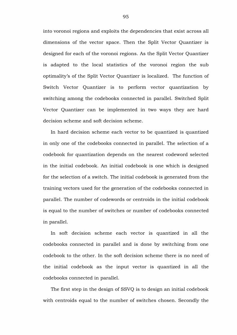
The first step in the design of SSVQ is to design an initial codebook

with centroids equal to the number of switches chosen. Secondly the

96

training vectors used for the generation of initial codebook are divided

into groups based on the nearest neighbor criterion. The training

vectors that are nearer to a centroid in the initial codebook must form

in one group. The number of groups is equal to the number of

centroids in the initial codebook.

Fig 4.9 Codebook training in Switched Split Vector Quantizer

In hard decision scheme the training of a codebook is shown in Fig

4.9. In Fig 4.9 mi i 1{C } corresponds to the centroids or codewords in

the initial codebook, „s ‟ corresponds to the vector to be quantized and

i=1, 2,….., m corresponds to the number of switching directions.

The block diagram of a Switched Split Vector Quantizer is shown in

Fig 4.10. From Fig 4.10 it is observed that a Split Vector Quantizer is

connected at each switch of SSVQ. The vector „s ‟ to be quantized is

switched to one of the quantizers connected in parallel. The switch

LBG

LBG

LBG

LBG

LBG

LBG

LBG

LBG

LBG

m

2

1

Split VQ 1

Codebooks

Split VQ 2

Codebooks

Split VQ m

Codebooks

s

Switch

Selection

Switch VQ Codebook

LBG

m

i i 1{C }

m

i i 1{C }

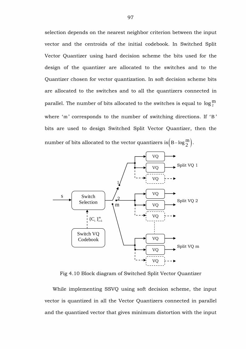
97

selection depends on the nearest neighbor criterion between the input

vector and the centroids of the initial codebook. In Switched Split

Vector Quantizer using hard decision scheme the bits used for the

design of the quantizer are allocated to the switches and to the

Quantizer chosen for vector quantization. In soft decision scheme bits

are allocated to the switches and to all the quantizers connected in

parallel. The number of bits allocated to the switches is equal to 2mlog

where „ m ‟ corresponds to the number of switching directions. If „ B ‟

bits are used to design Switched Split Vector Quantizer, then the

number of bits allocated to the vector quantizers is mB log2

.

Fig 4.10 Block diagram of Switched Split Vector Quantizer

While implementing SSVQ using soft decision scheme, the input

vector is quantized in all the Vector Quantizers connected in parallel

and the quantized vector that gives minimum distortion with the input

VQ

VQ

VQ

VQ

VQ

VQ

VQ

VQ

VQ

m

2

1

Split VQ 1

Split VQ 2

Split VQ m

Switch

Selection

Switch VQ

Codebook

m

i i 1{C }

s

98

vector is taken as the quantized version of the input vector. It is

expected that using soft decision scheme there is a slight decrease in

the spectral distortion as the input vector is quantized using more

than one vector quantizer, computational complexity and memory

requirements compared to hard decision scheme as the bits allocated

to the vector quantizer are distributed to all the quantizers connected

in parallel. So the number of bits at each quantizer is less in soft

decision scheme compared to the bits available at a quantizer in hard

decision scheme. As the number of available bits at each independent

quantizer decreases the complexity and memory requirements

decreases. The problem with SSVQ soft decision scheme is that using

soft decision scheme the reduction in bit-rate is inversely proportional

to the number of switches, number of quantizers connected in parallel

and number of splits, so it is not used.

In this work a 2- switch 3-part Switched Split Vector Quantizer

using hard decision scheme is implemented and its performance is

compared with other product code vector quantization schemes. From

results it is observed that Switched Split Vector Quantization using

hard decision scheme is having less spectral distortion and

computational complexity compared to Split Vector Quantization and

Multistage Vector Quantization techniques, but compared to Split-

Multistage Vector Quantization technique the spectral distortion and

computational complexity are high. The memory requirements of

Switched Split Vector Quantization using hard decision scheme is

better than Multistage Vector Quantization technique but is more

99

than Split Vector Quantization technique and Split-Multistage Vector

Quantization techniques [54, 81-85].

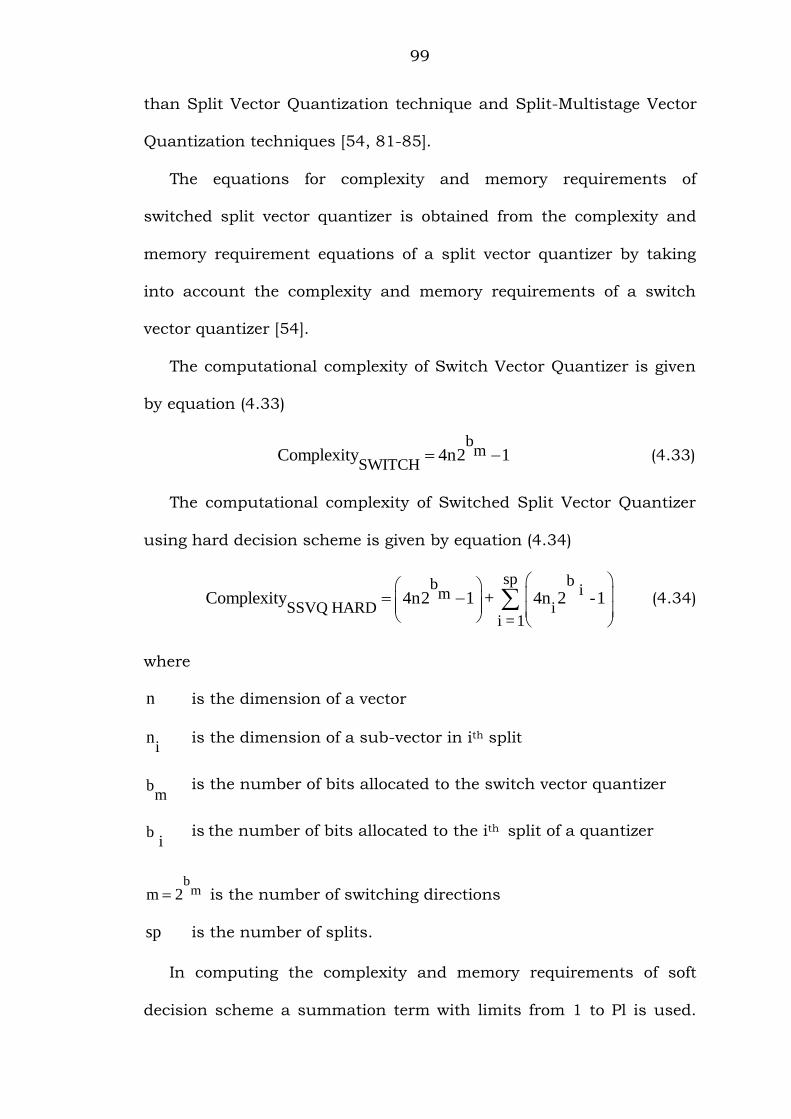
The equations for complexity and memory requirements of

switched split vector quantizer is obtained from the complexity and

memory requirement equations of a split vector quantizer by taking

into account the complexity and memory requirements of a switch

vector quantizer [54].

The computational complexity of Switch Vector Quantizer is given

by equation (4.33)

bm

SWITCHComplexity 4n2 1 (4.33)

The computational complexity of Switched Split Vector Quantizer

using hard decision scheme is given by equation (4.34)

sp bb imSSVQ HARD i

i = 1

Complexity 4n2 1 + 4n 2 -1

(4.34)

where

n is the dimension of a vector

in is the dimension of a sub-vector in ith split

bm

is the number of bits allocated to the switch vector quantizer

bi

is the number of bits allocated to the ith split of a quantizer

bmm 2 is the number of switching directions

sp is the number of splits.

In computing the complexity and memory requirements of soft

decision scheme a summation term with limits from 1 to Pl is used.

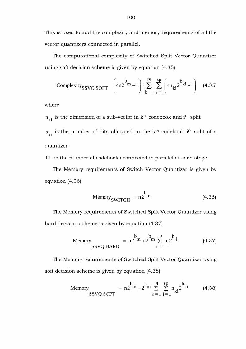
100

This is used to add the complexity and memory requirements of all the

vector quantizers connected in parallel.

The computational complexity of Switched Split Vector Quantizer

using soft decision scheme is given by equation (4.35)

spPlb bm ki

SSVQ SOFT kik 1 i = 1

Complexity 4n2 1 + 4n 2 -1

(4.35)

where

nki

is the dimension of a sub-vector in kth codebook and ith split

bki

is the number of bits allocated to the kth codebook ith split of a

quantizer

Pl is the number of codebooks connected in parallel at each stage

The Memory requirements of Switch Vector Quantizer is given by

equation (4.36)

bm

SWITCHMemory n2

(4.36)

The Memory requirements of Switched Split Vector Quantizer using

hard decision scheme is given by equation (4.37)

spb b b

m m i i

SSVQ HARD i = 1

Memory n2 2 n 2 (4.37)

The Memory requirements of Switched Split Vector Quantizer using

soft decision scheme is given by equation (4.38)

spPlb b b

m m ki ki

k 1SSVQ SOFT i =1

Memory n2 2 n 2

(4.38)

101

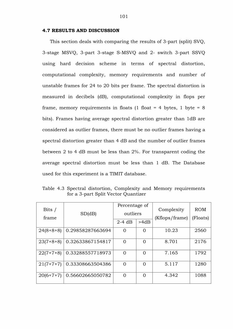
4.7 RESULTS AND DISCUSSION

This section deals with comparing the results of 3-part (split) SVQ,

3-stage MSVQ, 3-part 3-stage S-MSVQ and 2- switch 3-part SSVQ

using hard decision scheme in terms of spectral distortion,

computational complexity, memory requirements and number of

unstable frames for 24 to 20 bits per frame. The spectral distortion is

measured in decibels (dB), computational complexity in flops per

frame, memory requirements in floats (1 float = 4 bytes, 1 byte = 8

bits). Frames having average spectral distortion greater than 1dB are

considered as outlier frames, there must be no outlier frames having a

spectral distortion greater than 4 dB and the number of outlier frames

between 2 to 4 dB must be less than 2%. For transparent coding the

average spectral distortion must be less than 1 dB. The Database

used for this experiment is a TIMIT database.

Table 4.3 Spectral distortion, Complexity and Memory requirements

for a 3-part Split Vector Quantizer

Bits /

frame SD(dB)

Percentage of

outliers Complexity

(Kflops/frame)

ROM

(Floats) 2-4 dB >4dB

24(8+8+8) 0.29858287663694 0 0 10.23 2560

23(7+8+8) 0.32633867154817 0 0 8.701 2176

22(7+7+8) 0.33288557718973 0 0 7.165 1792

21(7+7+7) 0.33308663504386 0 0 5.117 1280

20(6+7+7) 0.56602665050782 0 0 4.342 1088

102

Table 4.4 Spectral distortion of a 3-part Split Vector Quantizer for

different priorities

Bits / frame SD(dB) Bits / frame SD(dB)

23(7+8+8) 0.31882128111235 23(8+7+8) 0.39490702824897

22(7+7+8) 0.33288557718973 22(7+8+7) 0.33653566762748

20(6+7+7) 0.56602665050782 20(7+7+6) 0.56696568993259

The bits allocated to each split of a 3-part SVQ are shown in the

brackets of the first column of Table 4.3. The number of splits taken is

3 with 3, 3, 4 dimensions each. The allocation of the bits to a

particular split depends on the priority given to that split. Splits with

high frequency LSFs are given more priority. The order of priority

given to the splits is split 1 < split 2 < split 3. From Table 4.4 it can be

observed that when the priority is altered the spectral distortion is

slightly increasing.

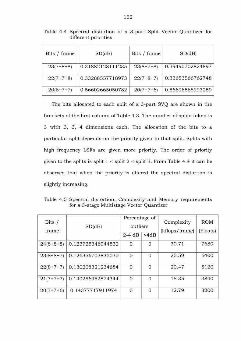
Table 4.5 Spectral distortion, Complexity and Memory requirements

for a 3-stage Multistage Vector Quantizer

Bits /

frame SD(dB)

Percentage of

outliers Complexity

(kflops/frame)

ROM

(Floats) 2-4 dB >4dB

24(8+8+8) 0.123725346044532 0 0 30.71 7680

23(8+8+7) 0.126356703835030 0 0 25.59 6400

22(8+7+7) 0.130208321234684 0 0 20.47 5120

21(7+7+7) 0.140256952874344 0 0 15.35 3840

20(7+7+6) 0.14377717911974 0 0 12.79 3200

103

Table 4.6 Spectral distortion of a 3-stage Multistage Vector Quantizer

for different priorities

Bits / frame SD(dB) Bits / frame SD(dB)

23(8+8+7) 0.126356703835030 23(7+8+8) 0.12777740330988

22(8+7+7) 0.130208321234684 22(7+7+8) 0.13857613575242

20(7+7+6) 0.14377717911974 20(6+7+7) 0.14634699335046

The bits allocated to each stage of a 3-stage MSVQ are shown in

the brackets of the first column of Table 4.5. The priority given to the

stages during the allocation of bits is stage 1 > stage 2 > stage 3.

Stages 2 and 3 are given less priority due to the quantization of errors.

It can be observed from Table 4.6 if the priority is not maintained the

spectral distortion is increasing.

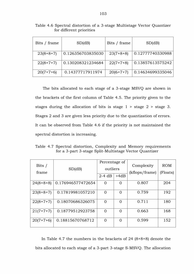
Table 4.7 Spectral distortion, Complexity and Memory requirements

for a 3-part 3-stage Split-Multistage Vector Quantizer

Bits /

frame SD(dB)

Percentage of

outliers Complexity

(kflops/frame)

ROM

(Floats) 2-4 dB >4dB

24(8+8+8) 0.176946577472654 0 0 0.807 204

23(8+8+7) 0.17819981057210 0 0 0.759 192

22(8+7+7) 0.18070686326075 0 0 0.711 180

21(7+7+7) 0.18779512923758 0 0 0.663 168

20(7+7+6) 0.18815670768712 0 0 0.599 152

In Table 4.7 the numbers in the brackets of 24 (8+8+8) denote the

bits allocated to each stage of a 3-part 3-stage S-MSVQ. The allocation

104

of the bits to a particular stage and split depends on the priority given

to that stage and split. The bits allocated to a stage are divided among

the splits of that stage.

Table 4.8 Spectral distortion, Complexity and Memory requirements for a 2-switch 3-part Switched Split Vector Quantizer using

hard decision scheme

Bits / frame SD(dB)

Percentage of

outliers

Complexity

(kflops/frame)

ROM

(Floats)

2-4 dB >4dB

24(1+7+8+8) 0.15197244909408 0 0 8.78 4372

23(1+7+7+8) 0.17666924153180 0 0 7.244 3604

22(1+7+7+7) 0.17983792575196 0 0 5.196 2580

21(1+6+7+7) 0.18376366181869 0 0 4.428 2196

20(1+6+6+7) 0.18376732214826 0 0 3.66 1812

In Table 4.8 the numbers in the brackets of 24 (1+7+8+8)

denote the bits allocated to the switches and splits of a 2- switch 3-

part SSVQ using hard decision scheme. The number of bits allocated

to a switch will depend on the number of switches chosen. The

number of bits allocated to the switches is equal to number of switches2log .

In this technique 2 switches are taken so the number of bits allocated

is 1, which is the first number in bracket. The allocation of the bits to

the splits of a quantizer is similar to the allocation of bits for the splits

in SVQ. In this technique two quantizers are connected in parallel and

the bits are allocated to the quantizer selected.

105

Table 4.9 Number of unstable frames for 3-part SVQ, 3-part 3-stage S-

MSVQ and 2-switch 3-part SSVQ using hard decision scheme with no ordering constraint

Bits / frame No of unstable frames

SVQ S-MSVQ SSVQ hard

24 0 1 0

23 0 1 6

22 0 1 6

21 0 1 6

20 0 1 6

Table 4.9 gives the number of unstable frames for 3-part SVQ, 3-

part 3-stage S-MSVQ and 2-switch 3-part SSVQ using hard decision

scheme. The instability is due to independent quantization of the sub-

vectors. This instability of frames is high at lower bit-rates. A frame is

said to be unstable when the line spectral frequencies of a vector

doesn‟t obey the ordering property.

20 20.5 21 21.5 22 22.5 23 23.5 240.1

0.15

0.2

0.25

0.3

0.35

0.4

0.45

0.5

0.55

0.6

Number of Bits/ Frame

Spe

ctra

l Dis

tort

ion

(dB

)

Spectral distortion for SVQ,MSVQ,S-MSVQ,SSVQ HARD

SVQ

S-MSVQ MSVQ SSVQ HARD

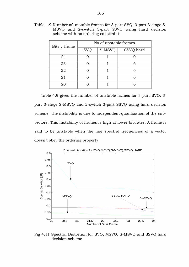
Fig 4.11 Spectral Distortion for SVQ, MSVQ, S-MSVQ and SSVQ hard decision scheme

106

The Fig 4.11 gives a plot of the spectral distortion of 3-part Split

Vector Quantizer, 3-stage Multistage Vector Quantizer, 3-part 3-stage

Split-Multistage Vector Quantizer, and 2-switch 3-part Switched Split

Vector Quantizer using hard decision scheme for 24 to 20 bits per

frame. The spectral distortion is measured in dB.

8 10 12 14 16 18 20 22 240

5

10

15

20

25

30

35

Number of bits/ frame

Com

ple

xity (

kflops/f

ram

e)

Complexity for SVQ, MSVQ, S-MSVQ,

SSVQ HARD DECISION SCHEME

SVQ

MSVQ

S-MSVQ

SSVQ HARD

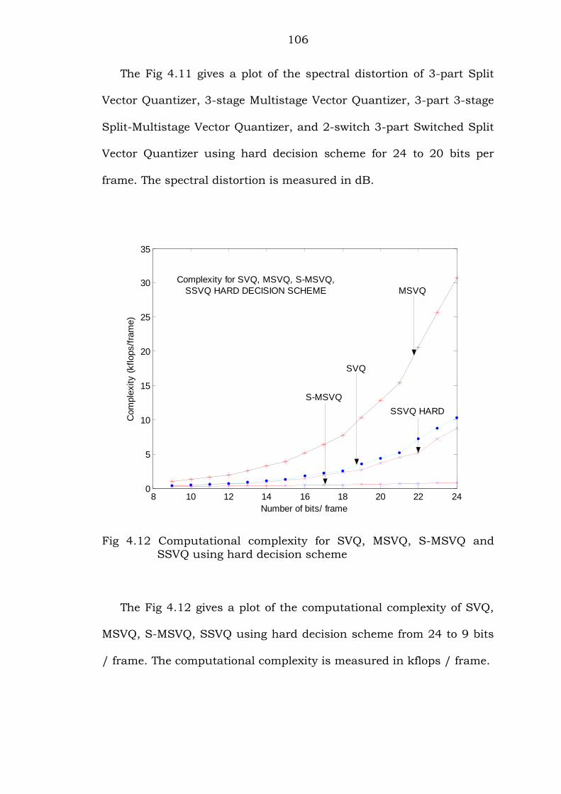
Fig 4.12 Computational complexity for SVQ, MSVQ, S-MSVQ and

SSVQ using hard decision scheme

The Fig 4.12 gives a plot of the computational complexity of SVQ,

MSVQ, S-MSVQ, SSVQ using hard decision scheme from 24 to 9 bits

/ frame. The computational complexity is measured in kflops / frame.

107

8 10 12 14 16 18 20 22 240

1000

2000

3000

4000

5000

6000

7000

8000

Number of bits/ frame

Mem

ory

Requirem

ents

(flo

ats

)

Memory Requirements for SVQ, MSVQ, S-MSVQ,

SSVQ HARD DECISION SCHEME

MSVQ

SSVQ HARD

SVQ

S-MSVQ

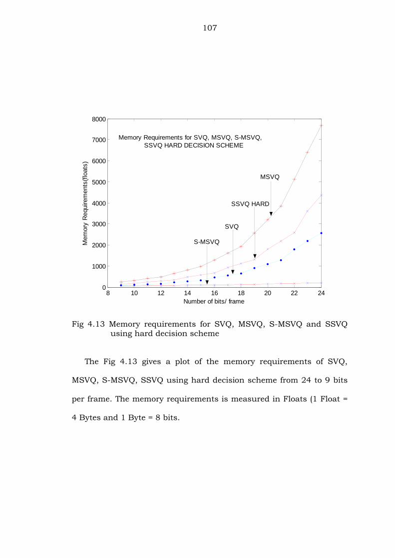
Fig 4.13 Memory requirements for SVQ, MSVQ, S-MSVQ and SSVQ

using hard decision scheme

The Fig 4.13 gives a plot of the memory requirements of SVQ,

MSVQ, S-MSVQ, SSVQ using hard decision scheme from 24 to 9 bits

per frame. The memory requirements is measured in Floats (1 Float =

4 Bytes and 1 Byte = 8 bits.

108

20 20.5 21 21.5 22 22.5 23 23.5 24-1

-0.8

-0.6

-0.4

-0.2

0

0.2

0.4

0.6

0.8

1

Number of Bits/ Frame

Outlie

rsOutliers 2 - 4 dB for SVQ,MSVQ,S-MSVQ,SSVQ HARD

SVQ

MSVQ

S-MSVQ

SSVQ

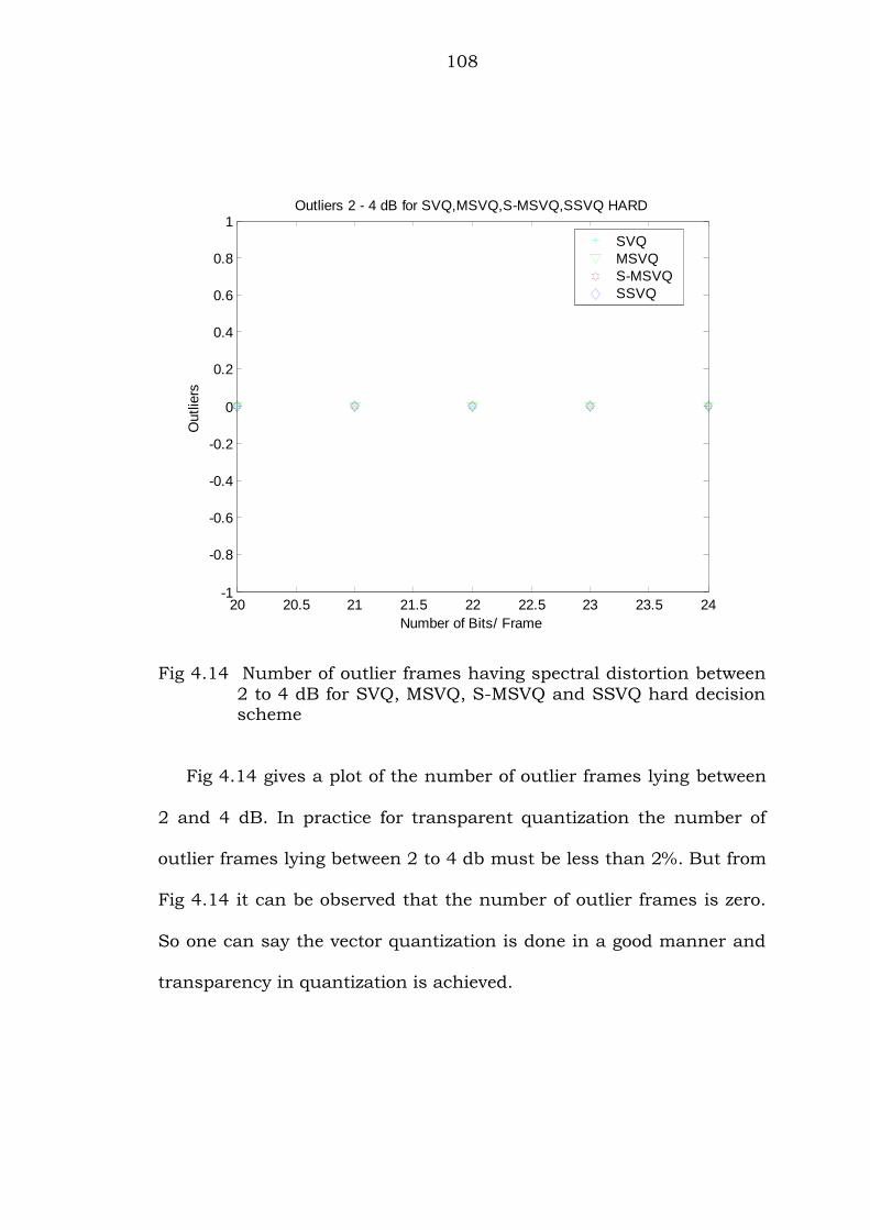
Fig 4.14 Number of outlier frames having spectral distortion between

2 to 4 dB for SVQ, MSVQ, S-MSVQ and SSVQ hard decision scheme

Fig 4.14 gives a plot of the number of outlier frames lying between

2 and 4 dB. In practice for transparent quantization the number of

outlier frames lying between 2 to 4 db must be less than 2%. But from

Fig 4.14 it can be observed that the number of outlier frames is zero.

So one can say the vector quantization is done in a good manner and

transparency in quantization is achieved.

109

20 20.5 21 21.5 22 22.5 23 23.5 24-1

-0.8

-0.6

-0.4

-0.2

0

0.2

0.4

0.6

0.8

1

Number of Bits/ Frame

Outlie

rs

Outliers Grater Than 4 dB for SVQ,MSVQ,S-MSVQ,SSVQ HARD

SVQ

MSVQ

S-MSVQ

SSVQ

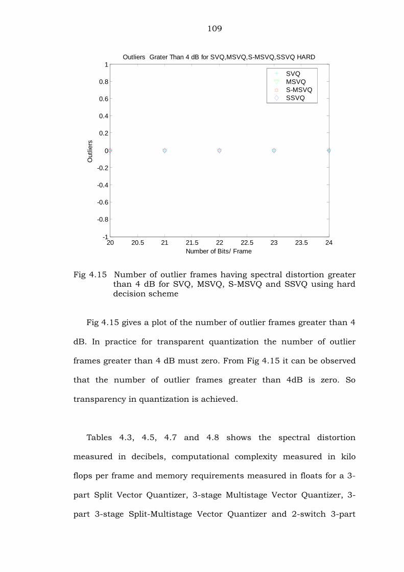
Fig 4.15 Number of outlier frames having spectral distortion greater than 4 dB for SVQ, MSVQ, S-MSVQ and SSVQ using hard

decision scheme

Fig 4.15 gives a plot of the number of outlier frames greater than 4

dB. In practice for transparent quantization the number of outlier

frames greater than 4 dB must zero. From Fig 4.15 it can be observed

that the number of outlier frames greater than 4dB is zero. So

transparency in quantization is achieved.

Tables 4.3, 4.5, 4.7 and 4.8 shows the spectral distortion

measured in decibels, computational complexity measured in kilo

flops per frame and memory requirements measured in floats for a 3-

part Split Vector Quantizer, 3-stage Multistage Vector Quantizer, 3-

part 3-stage Split-Multistage Vector Quantizer and 2-switch 3-part

110

Switched Split Vector Quantizer using hard decision scheme from 24

to 20 bits/frame. From Tables 4.3, 4.5, 4.7 and 4.8 and from Figs

4.11 to 4.13 it is concluded that 3-stage Multistage Vector Quantizer

is having less spectral distortion compared to 3-part Split Vector

Quantizer, 3-stage 3-part Split-Multistage Vector Quantizer and 2-

switch 3-part Switched Split Vector Quantizer using hard decision

scheme. Also it can be observed that 3-part 3-stage Split-Multistage

Vector Quantizer is having less computational complexity and memory

requirements compared to 3-part Split Vector Quantizer, 3-stage

Multistage Vector Quantizer and 2-switch 3-part Switched Split Vector

Quantizer using hard decision scheme. The lowest spectral distortion

for MSVQ is due to the addition of the quantized error vectors at each

stage to the quantized input vector at the first stage and due to the

preservation of correlation that exists between samples of a vector.

The decrease in the computational complexity and memory

requirements for S-MSVQ is due to the reduced dimension of vectors

to be quantized and due to the less availability of bits at each stage

and at each split of the vector quantizer.

Table 4.9 gives the number of unstable frames at a particular bit-

rate for a 3-part Split Vector Quantizer, 3-part 3-stage Split-

Multistage Vector Quantizer and 2-switch 3-part Switched Split Vector

Quantizer using hard decision scheme. The instability is due to

independent quantization of the sub-vectors (LSF) at each split. In

practice the number of unstable frames increases with a decrease in

the bit-rate which can be observed for 2-switch 3-part Switched Split

111

Vector Quantizer using hard decision scheme of Table 4.9. If there are

unstable frames after vector quantization the LPC synthesis filter

cannot be stable as the ascending order property of the LSF

coefficients in an LSF vector gets disturbed. So to prevent this, an

ordering constraint is imposed on the LSF parameters of each frame

which avoids the problem of unstable frames.

4.8 CONCLUSION

From results it is concluded that 3-stage Multistage Vector

Quantizer is having less spectral distortion when compared to Split

Vector Quantizer, Split-Multistage Vector Quantizer and Switched

Split Vector Quantizer using hard decision. The 3-part 3-stage Split-

Multistage Vector Quantizer is providing better tradeoff between bit-

rate and computational complexity, memory requirements when

compared to Split Vector Quantizer, Multistage Vector Quantizer,

Switched Split Vector Quantizer using hard decision scheme. Also

from results it is observed that the memory requirements of Switched

Split Vector Quantizer using hard decision scheme is more compared

to Split Vector Quantizer and this becomes the drawback of Switched

Split Vector Quantizer.