Distance learning in discriminative vectorquantization

Petra Schneider1, Michael Biehl1, Barbara Hammer2

1Institute for Mathematics and Computing Science, Universityof GroningenP.O. Box 407, 9700 AK Groningen, The Netherlands

p.schneider,m.biehl@rug.nl

2Institute of Computer Science, Clausthal University of TechnologyJulius Albert Strasse 4, 38678 Clausthal - Zellerfeld, Germany

hammer@in.tu-clausthal.de

Abstract

Discriminative vector quantization schemes such as learning vector quantiza-tion (LVQ) and extensions thereof offer efficient and intuitive classifiers whichare based on the representation of classes by prototypes. The originalmethods,however, rely on the Euclidean distance corresponding to the assumptionthat thedata can be represented by isotropic clusters. For this reason, extensions of themethods to more general metric structures have been proposed such as relevanceadaptation in generalized LVQ (GLVQ) and matrix learning in GLVQ In these ap-proaches, metric parameters are learned based on the given classification task suchthat a data driven distance measure is found. In this article, we considerfull matrixadaptation in advanced LVQ schemes; in particular, we introduce matrix learningto a recent statistical formalization of LVQ, robust soft LVQ, and we compare theresults on several artificial and real life data sets to matrix learning in GLVQ, whichconstitutes a derivation of LVQ-like learning based on a (heuristic) cost function.In all cases, matrix adaptation allows a significant improvement of the classifica-tion accuracy. Interestingly, however, the principled behavior of the models withrespect to prototype locations and extracted matrix dimensions shows several char-acteristic differences depending on the data sets.

Keywords: learning vector quantization, generalized LVQ, robust soft LVQ, met-ric adaptation

1 Introduction

Discriminative vector quantization schemes such as learning vector quantization (LVQ)constitute very popular classification methods due to theirintuitivity and robustness:they represent the classification by (usually few) prototypes which constitute typicalrepresentatives of the respective classes and, thus, allowa direct inspection of the givenclassifier. Training often takes place by Hebbian learning such that very fast and simpletraining algorithms result. Further, unlike the perceptron or the support vector machine,

1

LVQ provides an integrated and intuitive classification model for any given number ofclasses. Numerous modifications of original LVQ exist whichextend the basic learningscheme as proposed by Kohonen towards adaptive learning rates, faster convergence,or better approximation of Bayes optimal classification, toname just a few [9]. Despitetheir popularity and efficiency, most LVQ schemes are solelybased on heuristics anda deeper mathematical investigation of the models has just recently been initiated. Onthe one hand, their worst case generalization capability can be limited in terms of gen-eral margin bounds using techniques from computational learning theory [6, 5]. On theother hand, the characteristic behavior and learning curves of popular models can ex-actly be investigated in typical model situations using thetheory of online learning [3].Many questions, however, remain unsolved such as convergence and typical prototypelocations of heuristic LVQ schemes in concrete, finite training settings.Against this background, researchers have proposed variants of LVQ which can di-rectly be derived from an underlying cost function which is optimized during train-ing e.g. by means of a stochastic gradient ascent/descent. Generalized LVQ (GLVQ)as proposed by Sato and Yamada constitutes one example [11]:Its intuitive (thoughheuristic) cost function can be related to a minimization ofclassification errors and, atthe same time, a maximization of the hypothesis margin of theclassifier which charac-terizes its generalization ability [6]. The resulting algorithm is indeed very robust andpowerful, however, an exact mathematical analysis is stilllacking. A very elegant andmathematically well-founded alternative has been proposed by Seo and Obermayer:In [13], a statistical approach is introduced which models given classes as mixturesof Gaussians. Prototype parameters are optimized by maximizing the likelihood ratioof correct versus incorrect classification. A learning scheme which closely resemblesLVQ2.1 results. This cost function, however, is unbounded such that numerical insta-bilities occur which, in practice, cause the necessity of restricting updates to data froma windowclose to the decision boundary. The approach of [13] offers an elegant alter-native: A robust optimization scheme is derived from a maximization of the likelihoodratio of the probability of correct classification versus the total probability in a Gaus-sian mixture model. The resulting learning scheme, robust soft LVQ (RSLVQ), leadsto an alternative discrete LVQ scheme where prototypes are adapted solely based onmisclassifications.RSLVQ constitutes a very attractive model due to the fact that all underlying modelassumptions are stated explicitly in the statistical formulation – and they can easily bechanged if required by the application scenario. Besides, the resulting model showssuperior classification accuracy compared to GLVQ in a variety of settings as we willdemonstrate in this article.All these methods, however, suffer from the problem that classification is based ona predefined metric. The use of Euclidean distance, for instance, corresponds to theimplicit assumption of isotropic clusters. Such models canonly be successful if thedata displays a Euclidean characteristic. This is particularly problematic for high-dimensional data where noise accumulates and disrupts the classification, or hetero-geneous data sets where different scaling and correlationsof the dimensions can beobserved. Thus, a more general metric structure would be beneficial in such cases. Thefield of metric adaptation constitutes a very active research topic in various distancebased approaches such as unsupervised or semi-supervised clustering and visualiza-

2

tion [1, 8], k-nearest neighbor approaches [15, 16], and learning vectorquantization[7, 12]. We will focus on matrix learning in LVQ schemes whichaccounts for pair-wise correlations of features, i.e. a very general and flexible set of classifiers. On theone hand, we will investigate the behavior of generalized matrix LVQ in detail, a ma-trix adaptation scheme for GLVQ which is based on a heuristic, though intuitive costfunction. On the other hand, we will develop matrix adaptation for RSLVQ, a statisticalmodel for LVQ schemes, and thus we will arrive at a uniform statistical formulation forprototype and metric adaptation in discriminative prototype-based classifiers. We willintroduce variants which adapt the matrix parameters globally based on the training setor locally for every given prototype or mixture component, respectively.Matrix learning in RSLVQ and GLVQ will be evaluated and compared in a varietyof learning scenarios: First, we consider test scenarios where prior knowledge aboutthe form of the data is available. Furthermore, we compare the methods on severalbenchmarks from the UCI repository [10]. Finally, we demonstrate the benefit of ma-trix learning in a recent application from bioinformatics in the context of microarrayanalysis.Interestingly, depending on the data, the methods show different characteristic behav-ior with respect to prototype locations and learned metrics. Although the classificationaccuracy is in many cases comparable, they display quite different behavior concerningtheir robustness with respect to parameter choices and the characteristics of the solu-tions. We will point out that these findings have consequences on the interpretabilityof the results. In all cases, however, matrix adaptation leads to an improvement of theclassification accuracy, despite a largely increased number of free parameters.

2 Advanced learning vector quantization schemes

Learning vector quantization has been introduced by Kohonen [9], and a variety ofextensions and generalizations exist. Here we focus on approaches based on a costfunction, i.e. generalized learning vector quantization (GLVQ) and robust soft learningvector quantization (RSLVQ).Assume training dataξi, yi

li=1 ∈ R

N × 1, . . . , C are given,N denoting thedata dimensionality andC the number of different classes. An LVQ networkW =(wj , c(wj)) : R

N ×1, . . . , Cmj=1 consists of a numberm of prototypesw ∈ R

N

which are characterized by their location in feature space and their class labelc(w) ∈1 . . . , C. Classification is based on a winner takes all scheme. A data point ξ ∈ R

N

is mapped to the labelc(ξ) = c(wi) of the prototype, for whichd(ξ,wi) ≤ d(ξ,wj)holds∀j 6= i. Hered is an appropriate distance measure. Hence,ξ is mapped to theclass of the closest prototype, the so-called winner. Often, d is chosen as the squaredEuclidean metric, i.e.d(ξ,w) = (ξ − w)T (ξ − w).LVQ algorithms aim at an adaptation of the prototypes such that a given data set isclassified as accurately as possible. The first LVQ schemes proposed heuristic adap-tation rules based on the principle of Hebbian learning, such asLVQ2.1, which, fora given data pointξ, adapts the closest prototypew+(ξ) with the same class labelc(w+(ξ)) = c(ξ) into the direction ofξ: ∆w+(ξ) = α · (ξ − w+(ξ)) and the clos-est incorrect prototypew−(ξ) with a different class labelc(w−(ξ)) 6= c(ξ) is moved

3

into the opposite direction:∆w− = −α · (ξ − w−(ξ)). Here,α > 0 is the learningrate. Since, often, LVQ2.1 shows divergent behavior, a window rule is introduced, andadaptation takes place only ifw+(ξ) andw−(ξ) are the closest two prototypes ofξ.Generalized LVQderives a similar update rule from the following cost function:

EGLVQ =

l∑

i=1

Φ

(d(ξi,w

+(ξi)) − d(ξi,w−(ξi))

d(ξi,w+(ξi)) + d(ξi,w

−(ξi))

)

(1)

Φ is a monotonic function such as the identity or the logistic function. The numer-ator of a single summand is negative if the classification ofξ is correct. Further, asmall value corresponds to a classification with large margin, i.e. large difference ofthe distance to the closest correct and incorrect prototype. In this sense, GLVQ tries tominimize the number of misclassifications and to maximize the margin of the classifi-cation. The denominator accounts for a scaling of the terms such that the arguments ofΦ are restricted to the interval(−1, 1) and numerical problems are avoided. The costfunction of GLVQ can be related to a compromise of the minimization of the trainingerror and the generalization ability of the classifier whichis determined by the hypoth-esis margin (see [5, 6]). The connection, however, is not exact. The update formulas ofGLVQ can be derived by means of the gradients ofEGLVQ (see [7] for the derivation).Interestingly, the resulting learning rule resembles LVQ2.1 in the sense that the adapta-tion of the magnitude ofE and which accounts for a better robustness of the algorithmcompared to LVQ2.1.Unlike GLVQ, robust soft learning vector quantizationis based on a statistical mod-elling of the situation which makes all assumptions explicit: The probability density ofthe underlying data distribution is described by a mixture model. Every componentjof the mixture is assumed to generate data which belongs to only one of theC classes.The probability density of the full data set is given by

p(ξ|W ) =

C∑

i=1

m∑

j:c(wj)=i

p(ξ|j)P (j) (2)

where the conditional densityp(ξ|j) is a function of prototypewj . For example, theconditional density can be chosen to have the normalized exponential formp(ξ|j) =K(j) ·exp f(ξ,wj , σ

2j ), and the priorP (j) can be chosen identical for every prototype

wj . RSLVQ aims at a maximization of the likelihood ratio:

ERSLVQ =l∑

i=1

log

(p(ξi, yi|W )

p(ξi|W )

)

(3)

wherep(ξi, yi|W ) is the probability density thatξi is generated by a mixture compo-nent of the correct classyi andp(ξi|W ) is the total probability density ofξi. Thisimplies,

p(ξi, yi|W ) =∑

j:c(wj)=yi

p(ξi|j)P (j), p(ξi|W ) =∑

j

p(ξi|j)P (j) (4)

4

The learning rule of RSLVQ is derived fromERSLVQ by a stochastic gradient ascent.Since the value ofERSLVQ depends on the position of all prototypes, the complete setof prototypes is updated in each learning step. The gradientof a summand ofERSLVQ

for data point(ξ, y) with respect to a prototypewj is given by (see the appendix)

∂

∂wj

(

logp(ξ, y|W )

p(ξ|W )

)

= δy,c(wj) (Py(j|ξ) − P (j|ξ))∂f(ξ,wj , σ

2j )

∂wj

− (1 − δy,c(wj))P (j|ξ)∂f(ξ,wj , σ

2j )

∂wj

(5)

where the Kronecker symbolδy,c(wj) tests whether the labelsy andc(wj) coincide.In the special case of a Gaussian mixture model withσ2

j = σ2 andP (j) = 1/m for allj, we obtain

f(ξ,w, σ2) =−d(ξ,w)

2σ2(6)

whered(ξ,w) is the distance measure between data pointξ and prototypew. OriginalRSLVQ is based on the squared Euclidean distance. This implies

f(ξ,w, σ2) = −(ξ − w)T (ξ − w)

2σ2,

∂f

∂w=

1

σ2(ξ − w) (7)

Substituting the derivative off in equation (5) yields the update rule for the prototypesin RSLVQ

∆wj =α1

σ2

(Py(j|ξ) − P (j|ξ))(ξ − wj), c(wj) = y−P (j|ξ)(ξ − wj), c(wj) 6= y

(8)

whereα1 > 0 is the learning rate. In the limit of vanishing softnessσ2, the learningrule reduces to an intuitive crisplearning from mistakes(LFM) scheme, as pointed outin [13]: In case of erroneous classification, the closest correct and the closest wrongprototype are adapted along the direction pointing to / fromthe considered data point.Thus, a learning scheme very similar to LVQ2.1 results, which reduces adaptation towrongly classified inputs close to the decision boundary. While the soft version asintroduced in [13] leads to a good classification accuracy aswe will see in experiments,the limit rule has some principled deficiencies as shown in [3].

3 Matrix learning in advanced LVQ schemes

The squared Euclidean distance gives rise to isotropic clusters, hence the metric is notappropriate if data dimensions show a different scaling or correlations. A more generalform can be obtained by extending the metric to a full matrix

dΛ(ξ,w) = (ξ − w)T Λ(ξ − w) (9)

whereΛ is anN × N -matrix which is restricted to positive definite forms to guaranteemetricity. We can achieve this by substitutingΛ = ΩT Ω, whereΩ ∈ R

M×N . Further,

5

to prevent degeneration, we restrict∑

i Λii =∑

ij Ω2ij to a fixed value, i.e. the sum

of eigenvalues is normalized. The normalization∑

i Λii = N includes the Euclideandistance as special case withΛ = 1, where1 is the identity matrix. In the following,without loss of generality, we chooseΩ to be quadratic and symmetric, i.e.Λ = ΩΩ.Since an optimal matrix is not known beforehand for a given classification task, weadaptΛ or Ω, respectively, during training. For this purpose, we substitute the distancein the cost functions of LVQ by the new measure

dΛ(ξ,w) =∑

i,j,k

(ξi − wi)ΩikΩkj(ξj − wj) (10)

Generalized matrix LVQ(GMLVQ) extends the cost functionEGLVQ by this moregeneral metric and adapts the matrix parametersΩij together with the prototypes bymeans of a stochastic gradient descent, see [12] for detailsof the derivation. Note thatthe constraint

∑

i Λii = const. is simply achieved by means of a normalization of thematrix after every adaptation step.It is possible to introduce one global matrixΩ which corresponds to a global trans-formation of the data space, or, alternatively, to introduce an individual matrixΩj forevery prototype. The latter corresponds to the possibilityto adapt individual ellipsoidalclusters around every prototype. In this case, the squared distance is computed by

d(ξ,wj) = (ξ − wj)T Λj(ξ − wj) (11)

We refer to the extension of GMLVQ with local relevance matrices by the termlocalGMLVQ(LGMLVQ) [12].Now, we extend RSLVQ by the more general metric introduce in equation (9). Theconditional density function obtains the formp(ξ|j) = K(j) · exp f(ξ,w, σ2,Ω) with

f(ξ,w, σ2,Ω) =−(ξ − w)T ΩT Ω(ξ − w)

2σ2, (12)

∂f

∂w=

1

σ2ΩT Ω(ξ − w) =

1

σ2Λ (ξ − w), (13)

∂f

∂Ωlm

= −1

σ2

(∑

j

(ξl − wl)Ωmj(ξj − wj)

+∑

i

(ξi − wi)Ωil(ξm − wm)

)

(14)

Combining equations (5) and (13) yields the new update rule for the prototypes:

∆wj =α1

σ2

(Py(j|ξ) − P (j|ξ)) Λ (ξ − wj), c(wj) = y−P (j|ξ) Λ (ξ − wj), c(wj) 6= y

(15)

6

Taking the derivative of the summandERSLVQ for training sample(ξ, y) with respectto the elementsΩlm leads us to the update rule (see the appendix)

∆Ωlm = −α2

σ2·

∑

j

[(

δy,c(wj) (Py(j|ξ) − P (j|ξ)) − (1 − δy,c(wj))P (j|ξ))

·

(

[Ω(ξ − wj)]m(ξl − wj,l) + [Ω(ξ − wj)]l(ξm − wj,m))]

(16)

whereα2 > 0 is the learning rate for the metric parameters. The algorithm based onthe update rules in equations (15) and (16) will be calledmatrix RSLVQ(MRSLVQ) inthe following. Similar to local matrix learning in GMLVQ, itis also possible to train anindividual matrixΛj for every prototype. With individual matrices attached to all pro-totypes, the modification of (15) which includes the local matricesΛj is accompaniedby (see the appendix)

∆Ωj,lm = −α2

σ2·

[(

δy,c(wj)(Py(j|ξ) − P (j|ξ)) − (1 − δy,c(wj))P (j|ξ))

·

(

[Ωj(ξ − wj)]m(ξl − wj,l) + [Ωj(ξ − wj)]l(ξm − wj,m))]

(17)

We term this learning rulelocal MRSLVQ(LMRSLVQ). Note that under the assump-tion of equal priorsP (j), the resulting classifier is still given by the standard LVQclassifier: ξ 7→ c(wj) for which dΛj

(ξ,wj) is minimum, since this mixture com-ponent displays the maximum probabilityp(ξ|j) ∼ p(ξ|j) · P (j) for equal priors.Interestingly, the generalization ability of this function class has been investigated in[12] including the possibility of adaptive local matrices.Worst case generalizationbounds which depend on the number of prototypes and the hypothesis margin, i.e. theminimum difference between the closest correct and wrong prototype, can be foundwhich are independent of the input dimensionality (in particular independent of thematrix dimensionality), such that good generalization capability can be expected fromthese classifiers. We will investigate this claim in severalexperiments. In addition, wewill have a look at the robustness of the methods with respectto hyperparameters, theinterpretability of the results, and the uniqueness of the learned matrices.Although GLVQ and RSLVQ constitute two of the most promisingtheoretical deriva-tions of LVQ schemes from global cost functions, they have sofar not been comparedin experiments. Further, matrix learning offers a strikingextension of RSLVQ since itextends the underlying Gaussian mixture model towards the general form of arbitrarycovariance matrices, which has not been introduced or tested so far. Thus, we are inter-ested in several aspects and questions which should be highlighted by the experiments:

• What is the performance of the methods on real life data sets ofdifferent charac-teristics? Can the theoretically motivated claim of good generalization ability be

7

substantiated by experiments?

• What is the robustness of the methods with respect to metaparameters such asσ2?

• Do the methods provide meaningful (representative) prototypes or does the pro-totype location change due to the specific learning rule in adiscriminativeap-proach?

• Are the extracted matrices meaningful? In how far do they differ between theapproaches?

• Do there exist systematic differences in the solutions found by RSLVQ andGLVQ (with / without matrix adaptation)?

We first test the methods on two artificial data sets where the underlying density isknown exactly, which are designed for the evaluation of matrix adaptation. Afterwards,we compare the algorithms on benchmarks from UCI [10]. Finally, we demonstrate thebenefit of matrix adaptation in a recent application in bioinformatics.

4 Experiments

With respect to parameter initialization and learning rateannealing, we use the sameprocedures in all experiments. The mean values of random subsets of training samplesselected from each class are chosen as initial states of the prototypes. The hyper-parameterσ2 is held constant in all experiments with RSLVQ, MRSLVQ and LocalMRSLVQ. The learning rates are continuously reduced in the course of learning. Weimplement a schedule of the form

αi(t) =αi

1 + c (t − 1)(18)

(i ∈ 1, 2) wheret counts the number training epochs. The factorc determines thespeed of annealing and is chosen individually for every application. To normalizethe relevance matrices after each learning step, we choose

∑

i Λii = 1 and initially setΛ = 1/N . Note that, in consequence, the Euclidean distance in RSLVQand GLVQ hasto be normalized to one as well to allow for a fair comparison with respect to learningrates. Accordingly, the RSLVQ- and GLVQ prototype updates and the functionf inequation (7) have to be weighted by1/N .

4.1 Artificial Data

In the first experiments, the algorithms are applied to the artificial data from [4] to il-lustrate the training of an LVQ-classifier based on the alternative cost functions withfixed and adaptive distance measure. The data sets 1 and 2 comprise three-class classi-fication problems in a two dimensional space. Each class is split into two clusters withsmall or large overlap, respectively (see Figure 1). We randomly select 2/3 of the datasamples of each class for training and use the remaining datafor testing. According

8

to the a priori known distributions, the data is representedby two prototypes per class.Since we observe that the algorithms based on the RSLVQ cost function are very sen-sitive with respect to the learning parameter settings, slightly smaller values are chosento train a classifier with (M)RSLVQ compared to G(M)LVQ. We use the settings

G(M)LVQ: α1 = 5 · 10−3, α2 = 5 · 10−4, c = 0.01(M)RSLVQ: α1 = 5 · 10−4, α2 = 5 · 10−5, c = 0.001

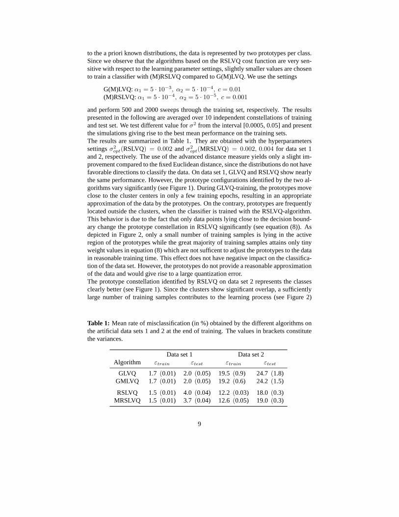
and perform 500 and 2000 sweeps through the training set, respectively. The resultspresented in the following are averaged over 10 independentconstellations of trainingand test set. We test different value forσ2 from the interval [0.0005, 0.05] and presentthe simulations giving rise to the best mean performance on the training sets.The results are summarized in Table 1. They are obtained withthe hyperparameterssettingsσ2

opt(RSLVQ) = 0.002 andσ2opt(MRSLVQ) = 0.002, 0.004 for data set 1

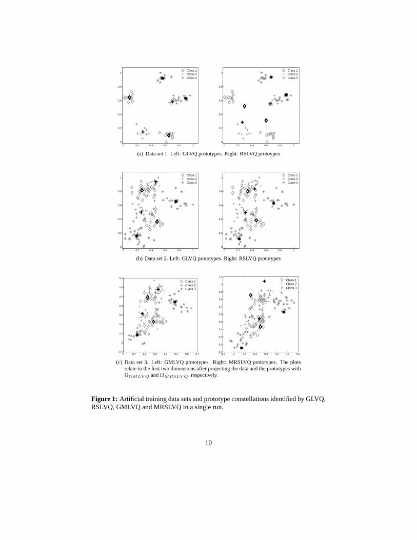
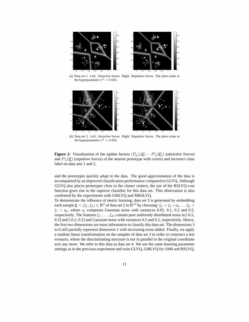
and 2, respectively. The use of the advanced distance measure yields only a slight im-provement compared to the fixed Euclidean distance, since the distributions do not havefavorable directions to classify the data. On data set 1, GLVQ and RSLVQ show nearlythe same performance. However, the prototype configurations identified by the two al-gorithms vary significantly (see Figure 1). During GLVQ-training, the prototypes moveclose to the cluster centers in only a few training epochs, resulting in an appropriateapproximation of the data by the prototypes. On the contrary, prototypes are frequentlylocated outside the clusters, when the classifier is trainedwith the RSLVQ-algorithm.This behavior is due to the fact that only data points lying close to the decision bound-ary change the prototype constellation in RSLVQ significantly (see equation (8)). Asdepicted in Figure 2, only a small number of training samplesis lying in the activeregion of the prototypes while the great majority of training samples attains only tinyweight values in equation (8) which are not sufficent to adjust the prototypes to the datain reasonable training time. This effect does not have negative impact on the classifica-tion of the data set. However, the prototypes do not provide areasonable approximationof the data and would give rise to a large quantization error.The prototype constellation identified by RSLVQ on data set 2represents the classesclearly better (see Figure 1). Since the clusters show significant overlap, a sufficientlylarge number of training samples contributes to the learning process (see Figure 2)

Table 1: Mean rate of misclassification (in %) obtained by the different algorithms onthe artificial data sets 1 and 2 at the end of training. The values in brackets constitutethe variances.

Data set 1 Data set 2Algorithm εtrain εtest εtrain εtest

GLVQ 1.7 (0.01) 2.0(0.05) 19.5(0.9) 24.7(1.8)GMLVQ 1.7 (0.01) 2.0(0.05) 19.2(0.6) 24.2(1.5)

RSLVQ 1.5 (0.01) 4.0(0.04) 12.2(0.03) 18.0(0.3)MRSLVQ 1.5 (0.01) 3.7(0.04) 12.6(0.05) 19.0(0.3)

9

0 0.2 0.4 0.6 0.8 10

0.2

0.4

0.6

0.8

1

Class 1Class 2Class 3

0 0.2 0.4 0.6 0.8 10

0.2

0.4

0.6

0.8

1

Class 1Class 2Class 3

(a) Data set 1. Left: GLVQ prototypes. Right: RSLVQ protoypes

0 0.2 0.4 0.6 0.8 10

0.2

0.4

0.6

0.8

1

Class 1Class 2Class 3

0 0.2 0.4 0.6 0.8 10

0.2

0.4

0.6

0.8

1

Class 1Class 2Class 3

(b) Data set 2. Left: GLVQ prototypes. Right: RSLVQ prototypes

0 0.1 0.2 0.3 0.4 0.5 0.6 0.7−0.1

0

0.1

0.2

0.3

0.4

0.5

0.6

0.7

Class 1Class 2Class 3

−0.1 0 0.1 0.2 0.3 0.4 0.5 0.60.1

0.2

0.3

0.4

0.5

0.6

0.7

0.8

0.9

1

1.1

Class 1Class 2Class 3

(c) Data set 3. Left: GMLVQ prototypes. Right: MRSLVQ prototypes. The plotsrelate to the first two dimensions after projecting the data and the prototypes withΩGMLV Q andΩMRSLV Q, respectively.

Figure 1: Artificial training data sets and prototype constellationsidentified by GLVQ,RSLVQ, GMLVQ and MRSLVQ in a single run.

10

0 0.2 0.4 0.6 0.8 1

0

0.2

0.4

0.6

0.8

1

0

0.1

0.2

0.3

0.4

0.5

0.6

0 0.2 0.4 0.6 0.8 1

0

0.2

0.4

0.6

0.8

1

0

0.1

0.2

0.3

0.4

0.5

0.6

(a) Data set 1. Left: Attractive forces. Right: Repulsive forces. The plots relate tothe hyperparameterσ2 = 0.002.

0 0.2 0.4 0.6 0.8 1

0

0.2

0.4

0.6

0.8

1

0

0.1

0.2

0.3

0.4

0.5

0.6

0.7

0 0.2 0.4 0.6 0.8 1

0

0.2

0.4

0.6

0.8

1

0

0.1

0.2

0.3

0.4

0.5

0.6

0.7

(b) Data set 2. Left: Attractive forces. Right: Repulsive forces. The plots relate tothe hyperparameterσ2 = 0.002.

Figure 2: Visualization of the update factors(Py(j|ξ) − P (j|ξ)) (attractive forces)andP (j|ξ) (repulsive forces) of the nearest prototype with correct and incorrect classlabel on data sets 1 and 2.

and the prototypes quickly adapt to the data. The good approximation of the data isaccompanied by an improved classification performance compared to GLVQ. AlthoughGLVQ also places prototypes close to the cluster centers, the use of the RSLVQ-costfunction gives rise to the superior classifier for this data set. This observation is alsoconfirmed by the experiments with GMLVQ and MRSLVQ.To demonstrate the influence of metric learning, data set 3 isgenerated by embeddingeach sampleξ = (ξ1, ξ2) ∈ R

2 of data set 2 inR10 by choosing:ξ3 = ξ1+η1, . . . ξ6 =ξ1 + η4, whereηi comprises Gaussian noise with variances 0.05, 0.1, 0.2 and 0.5,respectively. The featuresξ7, . . . , ξ10 contain pure uniformly distributed noise in [-0.5,0.5] and [-0.2, 0.2] and Gaussian noise with variances 0.5 and 0.2, respectively. Hence,the first two dimensions are most informative to classify this data set. The dimensions 3to 6 still partially represent dimension 1 with increasing noise added. Finally, we applya random linear transformation on the samples of data set 3 inorder to construct a testscenario, where the discriminating structure is not in parallel to the original coordinateaxis any more. We refer to this data as data set 4. We use the same learning parametersettings as in the previous experiment and train GLVQ, GMLVQfor 1000 and RSLVQ,

11

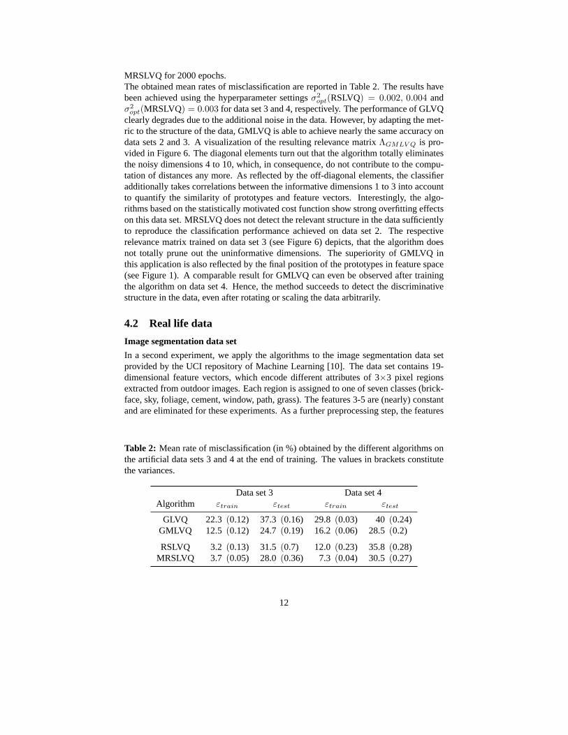
MRSLVQ for 2000 epochs.The obtained mean rates of misclassification are reported inTable 2. The results havebeen achieved using the hyperparameter settingsσ2

opt(RSLVQ) = 0.002, 0.004 andσ2

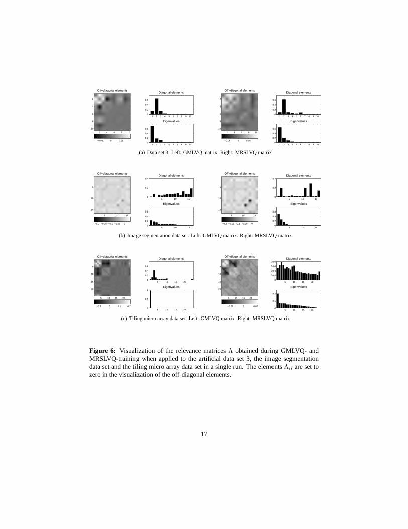
opt(MRSLVQ) = 0.003 for data set 3 and 4, respectively. The performance of GLVQclearly degrades due to the additional noise in the data. However, by adapting the met-ric to the structure of the data, GMLVQ is able to achieve nearly the same accuracy ondata sets 2 and 3. A visualization of the resulting relevancematrix ΛGMLV Q is pro-vided in Figure 6. The diagonal elements turn out that the algorithm totally eliminatesthe noisy dimensions 4 to 10, which, in consequence, do not contribute to the compu-tation of distances any more. As reflected by the off-diagonal elements, the classifieradditionally takes correlations between the informative dimensions 1 to 3 into accountto quantify the similarity of prototypes and feature vectors. Interestingly, the algo-rithms based on the statistically motivated cost function show strong overfitting effectson this data set. MRSLVQ does not detect the relevant structure in the data sufficientlyto reproduce the classification performance achieved on data set 2. The respectiverelevance matrix trained on data set 3 (see Figure 6) depicts, that the algorithm doesnot totally prune out the uninformative dimensions. The superiority of GMLVQ inthis application is also reflected by the final position of theprototypes in feature space(see Figure 1). A comparable result for GMLVQ can even be observed after trainingthe algorithm on data set 4. Hence, the method succeeds to detect the discriminativestructure in the data, even after rotating or scaling the data arbitrarily.

4.2 Real life data

Image segmentation data set

In a second experiment, we apply the algorithms to the image segmentation data setprovided by the UCI repository of Machine Learning [10]. Thedata set contains 19-dimensional feature vectors, which encode different attributes of 3×3 pixel regionsextracted from outdoor images. Each region is assigned to one of seven classes (brick-face, sky, foliage, cement, window, path, grass). The features 3-5 are (nearly) constantand are eliminated for these experiments. As a further preprocessing step, the features

Table 2: Mean rate of misclassification (in %) obtained by the different algorithms onthe artificial data sets 3 and 4 at the end of training. The values in brackets constitutethe variances.

Data set 3 Data set 4Algorithm εtrain εtest εtrain εtest

GLVQ 22.3 (0.12) 37.3(0.16) 29.8(0.03) 40 (0.24)GMLVQ 12.5 (0.12) 24.7(0.19) 16.2(0.06) 28.5(0.2)

RSLVQ 3.2 (0.13) 31.5(0.7) 12.0(0.23) 35.8(0.28)MRSLVQ 3.7 (0.05) 28.0(0.36) 7.3(0.04) 30.5(0.27)

12

are normalized to zero mean and unit variance. The provided data is split into a trainingand a test set (30 samples per class for training, 300 samplesper class for testing). Inorder to find useful values for the hyperparameter in RSLVQ and related methods, werandomly split the test data in a validation and a test set of equal size. The validationset is not used for the experiments with GMLVQ. Each class is approximated by oneprototype. We use the parameter settings

(Local) G(M)LVQ: α1 = 1 × 10−2, α2 = 1 × 10−3, c = 0.1(Local) (M)RSLVQ:α1 = 1 × 10−3, α2 = 1 × 10−4, c = 1 × 10−3

and test values forσ2 in the interval [0.005, 0.3]. The algorithms are trained for1400epochs in total. In the following, we always refer to the experiments with the hyperpa-rameter resulting in the best performance on the validationset. The respective valuesareσ2

opt(RSLVQ) = 0.01, σ2opt(MRSLVQ) = 0.05 andσ2

opt(LMRSLVQ) = 0.065.The obtained classification accuracies are summarized in Table 3. For both cost func-tion schemes the performance improves with increasing complexity of the distancemeasure, except for Local MRSLVQ which shows overfitting effects. Remarkably,RSLVQ and MRSLVQ clearly outperform the respective GLVQ methods on this dataset. Regarding GLVQ and RSLVQ, this observation is solely based on different pro-totype constellations. The algorithms identify similarw for classes with low rate ofmisclassification. Differences can be observed in case of prototypes, which contributestrongly to the overall test error. For demonstration purposes, we refer to classes 5 and7. The mean class specific test errors constituteε5

test = 0.4 andε7test = 0.01 for the

GLVQ classifiers andε5test = 0.19 andε7

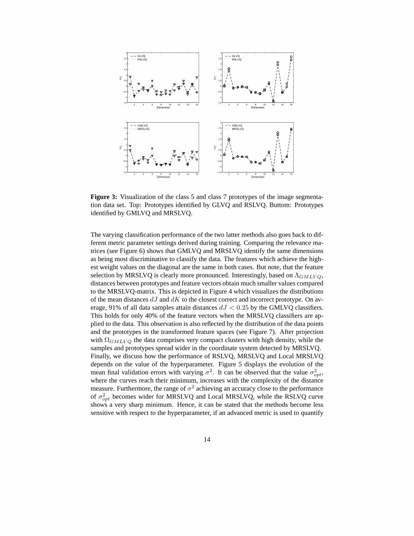
test = 0.01 for the RSLVQ classifiers. Therespective prototypes obtained in one cross validation runare visualized in Figure 3.It depicts that the algorithms identify nearly the same representative for class 7, whilethe class 5 prototypes reflect differences for the alternative learning strategies. Thisfinding holds similarly for the GMLVQ and MRSLVQ prototypes,however, it is lesspronounced (see Figure 3).

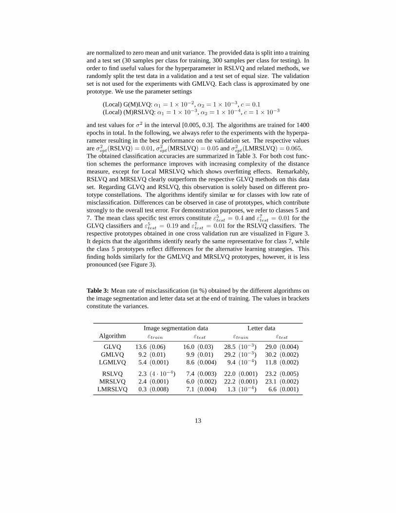
Table 3: Mean rate of misclassification (in %) obtained by the different algorithms onthe image segmentation and letter data set at the end of training. The values in bracketsconstitute the variances.

Image segmentation data Letter dataAlgorithm εtrain εtest εtrain εtest

GLVQ 13.6 (0.06) 16.0(0.03) 28.5(10−3) 29.0 (0.004)GMLVQ 9.2 (0.01) 9.9(0.01) 29.2(10−3) 30.2 (0.002)

LGMLVQ 5.4 (0.001) 8.6(0.004) 9.4(10−4) 11.8 (0.002)

RSLVQ 2.3 (4 · 10−4) 7.4 (0.003) 22.0(0.001) 23.2(0.005)MRSLVQ 2.4 (0.001) 6.0(0.002) 22.2(0.001) 23.1(0.002)

LMRSLVQ 0.3 (0.008) 7.1(0.004) 1.3(10−4) 6.6 (0.001)

13

2 4 6 8 10 12 14 16−1.5

−1

−0.5

0

0.5

1

1.5

2

2.5

3

Dimension

w5

GLVQRSLVQ

2 4 6 8 10 12 14 16−1.5

−1

−0.5

0

0.5

1

1.5

2

2.5

3

Dimension

w7

GLVQRSLVQ

2 4 6 8 10 12 14 16−1.5

−1

−0.5

0

0.5

1

1.5

2

2.5

3

Dimension

w5

GMLVQMRSLVQ

2 4 6 8 10 12 14 16−1.5

−1

−0.5

0

0.5

1

1.5

2

2.5

3

Dimension

w7

GMLVQMRSLVQ

Figure 3: Visualization of the class 5 and class 7 prototypes of the image segmenta-tion data set. Top: Prototypes identified by GLVQ and RSLVQ. Buttom: Prototypesidentified by GMLVQ and MRSLVQ.

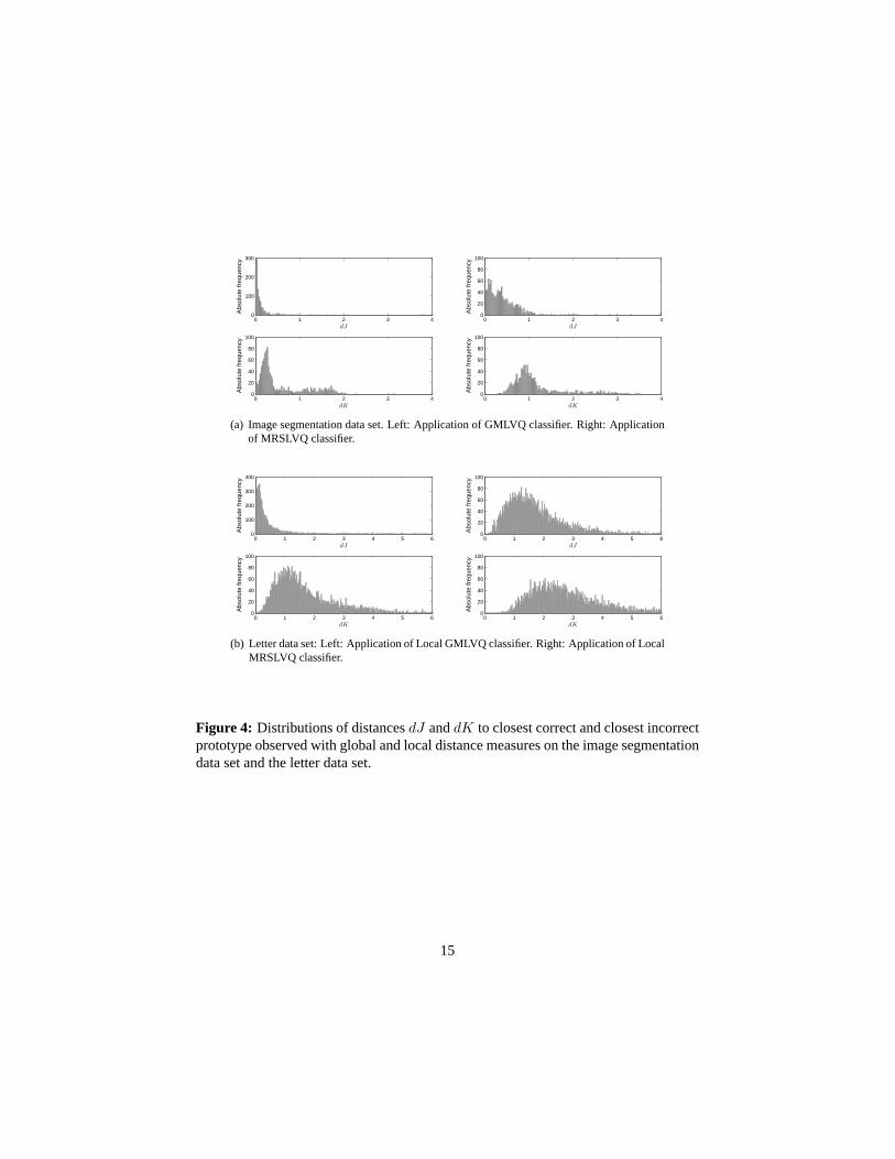
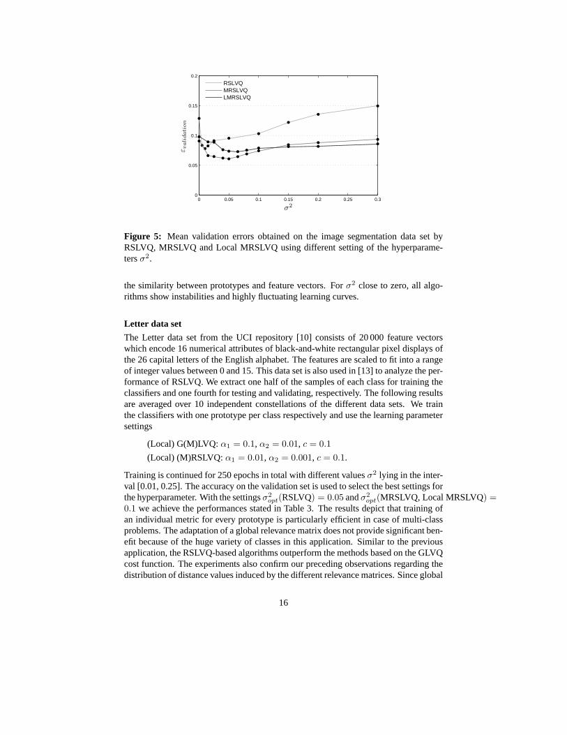
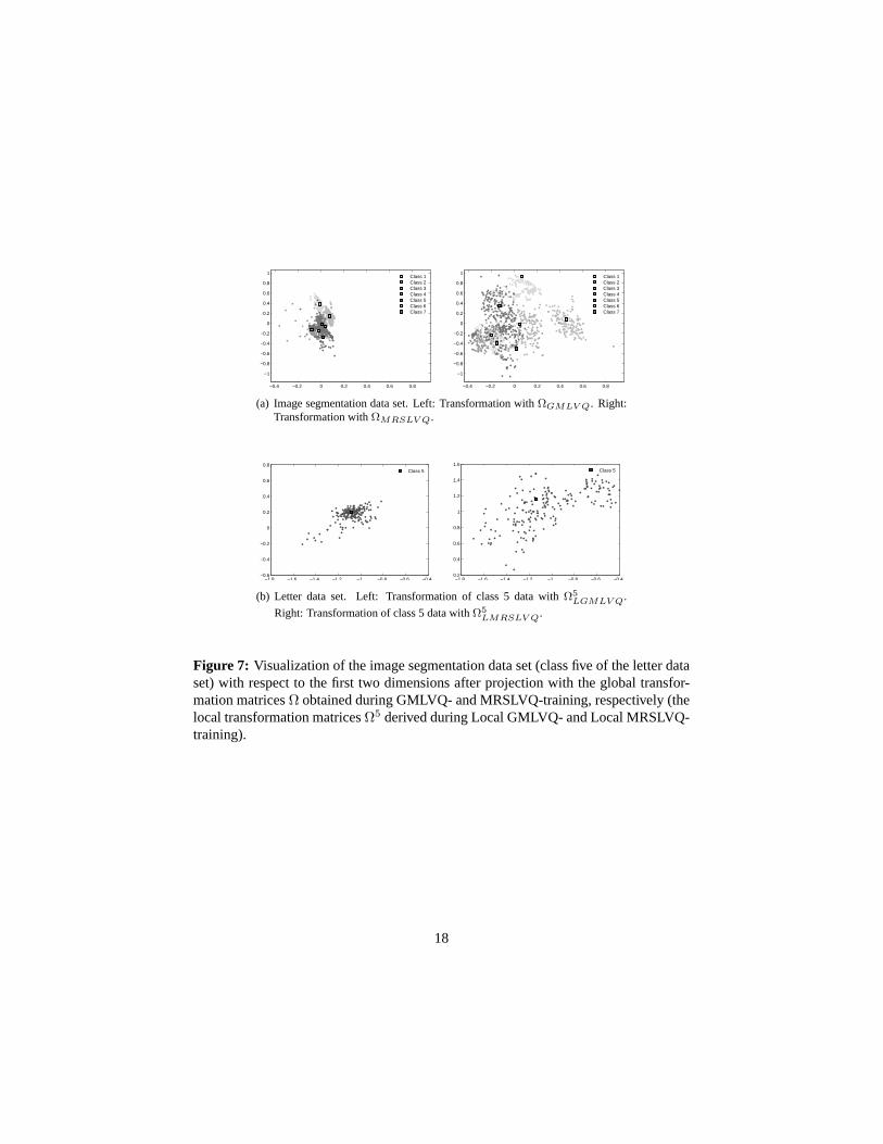
The varying classification performance of the two latter methods also goes back to dif-ferent metric parameter settings derived during training.Comparing the relevance ma-trices (see Figure 6) shows that GMLVQ and MRSLVQ identify the same dimensionsas being most discriminative to classify the data. The features which achieve the high-est weight values on the diagonal are the same in both cases. But note, that the featureselection by MRSLVQ is clearly more pronounced. Interestingly, based onΛGMLV Q,distances between prototypes and feature vectors obtain much smaller values comparedto the MRSLVQ-matrix. This is depicted in Figure 4 which visualizes the distributionsof the mean distancesdJ anddK to the closest correct and incorrect prototype. On av-erage, 91% of all data samples attain distancesdJ < 0.25 by the GMLVQ classifiers.This holds for only 40% of the feature vectors when the MRSLVQclassifiers are ap-plied to the data. This observation is also reflected by the distribution of the data pointsand the prototypes in the transformed feature spaces (see Figure 7). After projectionwith ΩGMLV Q the data comprises very compact clusters with high density,while thesamples and prototypes spread wider in the coordinate system detected by MRSLVQ.Finally, we discuss how the performance of RSLVQ, MRSLVQ andLocal MRSLVQdepends on the value of the hyperparameter. Figure 5 displays the evolution of themean final validation errors with varyingσ2. It can be observed that the valueσ2

opt,where the curves reach their minimum, increases with the complexity of the distancemeasure. Furthermore, the range ofσ2 achieving an accuracy close to the performanceof σ2

opt becomes wider for MRSLVQ and Local MRSLVQ, while the RSLVQ curveshows a very sharp minimum. Hence, it can be stated that the methods become lesssensitive with respect to the hyperparameter, if an advanced metric is used to quantify

14

0 1 2 3 40

100

200

300

dJ

Abs

olut

e fr

eque

ncy

0 1 2 3 40

20

40

60

80

100

Abs

olut

e fr

eque

ncy

dK

0 1 2 3 40

20

40

60

80

100

dJ

Abs

olut

e fr

eque

ncy

0 1 2 3 40

20

40

60

80

100

Abs

olut

e fr

eque

ncy

dK

(a) Image segmentation data set. Left: Application of GMLVQ classifier. Right: Applicationof MRSLVQ classifier.

0 1 2 3 4 5 60

100

200

300

400

dJ

Abs

olut

e fr

eque

ncy

0 1 2 3 4 5 60

20

40

60

80

100

Abs

olut

e fr

eque

ncy

dK

0 1 2 3 4 5 60

20

40

60

80

100

dJ

Abs

olut

e fr

eque

ncy

0 1 2 3 4 5 60

20

40

60

80

100

Abs

olut

e fr

eque

ncy

dK

(b) Letter data set: Left: Application of Local GMLVQ classifier. Right: Application of LocalMRSLVQ classifier.

Figure 4: Distributions of distancesdJ anddK to closest correct and closest incorrectprototype observed with global and local distance measureson the image segmentationdata set and the letter data set.

15

0 0.05 0.1 0.15 0.2 0.25 0.30

0.05

0.1

0.15

0.2

σ2

εvali

dati

on

RSLVQMRSLVQLMRSLVQ

Figure 5: Mean validation errors obtained on the image segmentation data set byRSLVQ, MRSLVQ and Local MRSLVQ using different setting of the hyperparame-tersσ2.

the similarity between prototypes and feature vectors. Forσ2 close to zero, all algo-rithms show instabilities and highly fluctuating learning curves.

Letter data set

The Letter data set from the UCI repository [10] consists of 20 000 feature vectorswhich encode 16 numerical attributes of black-and-white rectangular pixel displays ofthe 26 capital letters of the English alphabet. The featuresare scaled to fit into a rangeof integer values between 0 and 15. This data set is also used in [13] to analyze the per-formance of RSLVQ. We extract one half of the samples of each class for training theclassifiers and one fourth for testing and validating, respectively. The following resultsare averaged over 10 independent constellations of the different data sets. We trainthe classifiers with one prototype per class respectively and use the learning parametersettings

(Local) G(M)LVQ: α1 = 0.1, α2 = 0.01, c = 0.1

(Local) (M)RSLVQ:α1 = 0.01, α2 = 0.001, c = 0.1.

Training is continued for 250 epochs in total with differentvaluesσ2 lying in the inter-val [0.01, 0.25]. The accuracy on the validation set is used to select the best settings forthe hyperparameter. With the settingsσ2

opt(RSLVQ) = 0.05 andσ2opt(MRSLVQ, Local MRSLVQ) =

0.1 we achieve the performances stated in Table 3. The results depict that training ofan individual metric for every prototype is particularly efficient in case of multi-classproblems. The adaptation of a global relevance matrix does not provide significant ben-efit because of the huge variety of classes in this application. Similar to the previousapplication, the RSLVQ-based algorithms outperform the methods based on the GLVQcost function. The experiments also confirm our preceding observations regarding thedistribution of distance values induced by the different relevance matrices. Since global

16

Off−diagonal elements

2 4 6 8 10

2

4

6

8

10

−0.05 0 0.05

1 2 3 4 5 6 7 8 9 100

0.2

0.4

0.6

Diagonal elements

1 2 3 4 5 6 7 8 9 100

0.2

0.4

0.6

Eigenvalues

Off−diagonal elements

2 4 6 8 10

2

4

6

8

10

−0.05 0 0.05

1 2 3 4 5 6 7 8 9 100

0.2

0.4

0.6

Diagonal elements

1 2 3 4 5 6 7 8 9 100

0.2

0.4

0.6

Eigenvalues

(a) Data set 3. Left: GMLVQ matrix. Right: MRSLVQ matrix

Off−diagonal elements

5 10 15

5

10

15

−0.2 −0.15 −0.1 −0.05 0

5 10 150

0.2

0.4Diagonal elements

5 10 150

0.2

0.4

0.6

Eigenvalues

Off−diagonal elements

5 10 15

5

10

15

−0.2 −0.15 −0.1 −0.05 0

5 10 150

0.2

0.4Diagonal elements

5 10 150

0.2

0.4

0.6

Eigenvalues

(b) Image segmentation data set. Left: GMLVQ matrix. Right: MRSLVQ matrix

Off−diagonal elements

5 10 15 20

5

10

15

20

−0.1 0 0.1 0.2

5 10 15 200

0.2

0.4

0.6

Diagonal elements

5 10 15 200

0.5

1Eigenvalues

Off−diagonal elements

5 10 15 20

5

10

15

20

−0.02 0 0.02

5 10 15 200

0.02

0.04

0.06

0.08Diagonal elements

5 10 15 200

0.1

0.2

Eigenvalues

(c) Tiling micro array data set. Left: GMLVQ matrix. Right: MRSLVQ matrix

Figure 6: Visualization of the relevance matricesΛ obtained during GMLVQ- andMRSLVQ-training when applied to the artificial data set 3, the image segmentationdata set and the tiling micro array data set in a single run. The elementsΛii are set tozero in the visualization of the off-diagonal elements.

17

−0.4 −0.2 0 0.2 0.4 0.6 0.8

−1

−0.8

−0.6

−0.4

−0.2

0

0.2

0.4

0.6

0.8

1

Class 1Class 2Class 3Class 4Class 5Class 6Class 7

−0.4 −0.2 0 0.2 0.4 0.6 0.8

−1

−0.8

−0.6

−0.4

−0.2

0

0.2

0.4

0.6

0.8

1

Class 1Class 2Class 3Class 4Class 5Class 6Class 7

(a) Image segmentation data set. Left: Transformation withΩGMLV Q. Right:Transformation withΩMRSLV Q.

−1.8 −1.6 −1.4 −1.2 −1 −0.8 −0.6 −0.4−0.6

−0.4

−0.2

0

0.2

0.4

0.6

0.8

Class 5

−1.8 −1.6 −1.4 −1.2 −1 −0.8 −0.6 −0.40.2

0.4

0.6

0.8

1

1.2

1.4

1.6

Class 5

(b) Letter data set. Left: Transformation of class 5 data withΩ5

LGMLV Q.

Right: Transformation of class 5 data withΩ5

LMRSLV Q.

Figure 7: Visualization of the image segmentation data set (class fiveof the letter dataset) with respect to the first two dimensions after projection with the global transfor-mation matricesΩ obtained during GMLVQ- and MRSLVQ-training, respectively(thelocal transformation matricesΩ5 derived during Local GMLVQ- and Local MRSLVQ-training).

18

−15 −10 −5 0 5 100

10

20

30

dJ - dK

Abs

olut

e fr

eque

ncy

(a) Class conditional means

−15 −10 −5 0 5 100

10

20

30

Abs

olut

e fr

eque

ncy

dJ - dK

(b) GLVQ prototypes

−15 −10 −5 0 5 100

10

20

30

Abs

olut

e fr

eque

ncy

dJ - dK

(c) GMLVQ prototypes

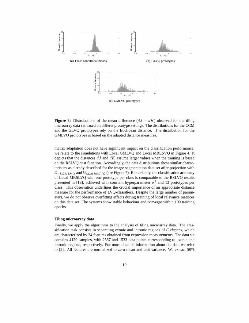
Figure 8: Distrubutions of the mean difference (dJ − dK) observed for the tilingmicroarray data set based on differet prototype settings. The distributions for the CCMand the GLVQ prototypes rely on the Euclidean distance. The distribution for theGMLVQ prototypes is based on the adapted distance measures.

matrix adaptation does not have significant impact on the classification performance,we relate to the simulations with Local GMLVQ and Local MRLSVQ in Figure 4. Itdepicts that the distancesdJ anddK assume larger values when the training is basedon the RSLVQ cost function. Accordingly, the data distributions show similar charac-teristics as already described for the image segmentation data set after projection withΩi,LGMLV Q andΩi,LMRSLV Q (see Figure 7). Remarkably, the classification accuracyof Local MRSLVQ with one prototype per class is comparable tothe RSLVQ resultspresented in [13], achieved with constant hyperparameterσ2 and 13 prototypes perclass. This observation underlines the crucial importanceof an appropriate distancemeasure for the performance of LVQ-classifiers. Despite thelarge number of param-eters, we do not observe overfitting effects during trainingof local relevance matriceson this data set. The systems show stable behaviour and converge within 100 trainingepochs.

Tiling microarray data

Finally, we apply the algorithms to the analysis of tiling microarray data. The clas-sification task consists in separating exonic and intronic regions ofC.elegans, whichare characterized by 24 features obtained from expression measurements. The data setcontains 4120 samples, with 2587 and 1533 data points corresponding to exonic andintronic regions, respectively. For more detailed information about the data we referto [2]. All features are normalized to zero mean and unit variance. We extract 50%

19

5 10 15 20−1

−0.5

0

0.5

1

1.5

2

Dimension

w1,2

GLVQGMLVQCCM

5 10 15 20−1

−0.5

0

0.5

1

1.5

2

Dimension

w1,2

RSLVQMRSLVQCCM

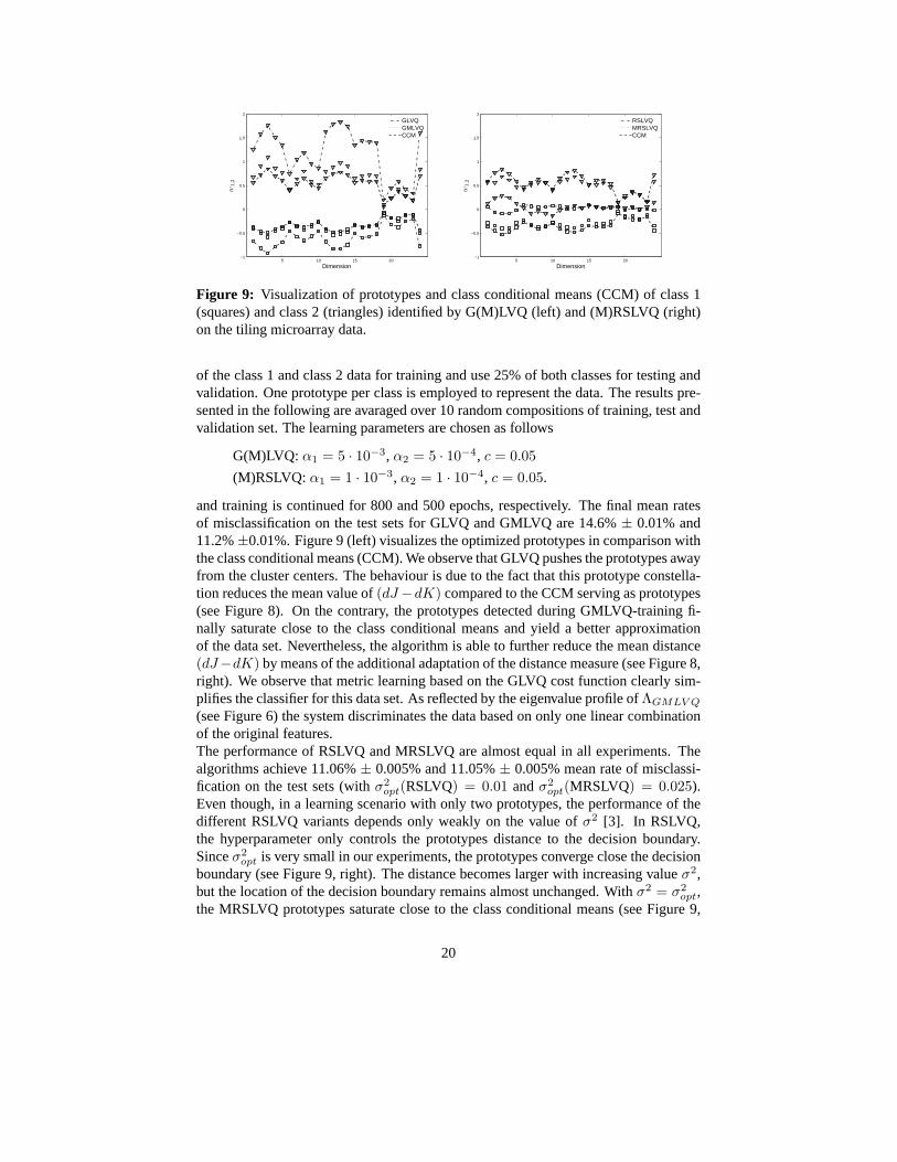
Figure 9: Visualization of prototypes and class conditional means (CCM) of class 1(squares) and class 2 (triangles) identified by G(M)LVQ (left) and (M)RSLVQ (right)on the tiling microarray data.

of the class 1 and class 2 data for training and use 25% of both classes for testing andvalidation. One prototype per class is employed to represent the data. The results pre-sented in the following are avaraged over 10 random compositions of training, test andvalidation set. The learning parameters are chosen as follows

G(M)LVQ: α1 = 5 · 10−3, α2 = 5 · 10−4, c = 0.05

(M)RSLVQ: α1 = 1 · 10−3, α2 = 1 · 10−4, c = 0.05.

and training is continued for 800 and 500 epochs, respectively. The final mean ratesof misclassification on the test sets for GLVQ and GMLVQ are 14.6%± 0.01% and11.2%±0.01%. Figure 9 (left) visualizes the optimized prototypesin comparison withthe class conditional means (CCM). We observe that GLVQ pushes the prototypes awayfrom the cluster centers. The behaviour is due to the fact that this prototype constella-tion reduces the mean value of(dJ −dK) compared to the CCM serving as prototypes(see Figure 8). On the contrary, the prototypes detected during GMLVQ-training fi-nally saturate close to the class conditional means and yield a better approximationof the data set. Nevertheless, the algorithm is able to further reduce the mean distance(dJ−dK) by means of the additional adaptation of the distance measure (see Figure 8,right). We observe that metric learning based on the GLVQ cost function clearly sim-plifies the classifier for this data set. As reflected by the eigenvalue profile ofΛGMLV Q

(see Figure 6) the system discriminates the data based on only one linear combinationof the original features.The performance of RSLVQ and MRSLVQ are almost equal in all experiments. Thealgorithms achieve 11.06%± 0.005% and 11.05%± 0.005% mean rate of misclassi-fication on the test sets (withσ2

opt(RSLVQ) = 0.01 andσ2opt(MRSLVQ) = 0.025).

Even though, in a learning scenario with only two prototypes, the performance of thedifferent RSLVQ variants depends only weakly on the value ofσ2 [3]. In RSLVQ,the hyperparameter only controls the prototypes distance to the decision boundary.Sinceσ2

opt is very small in our experiments, the prototypes converge close the decisionboundary (see Figure 9, right). The distance becomes largerwith increasing valueσ2,but the location of the decision boundary remains almost unchanged. Withσ2 = σ2

opt,the MRSLVQ prototypes saturate close to the class conditional means (see Figure 9,

20

right). Due to the additional adaptation of the metric, the prototypes distance to thedecision boundary increases only mildly with increasingσ2. Instead, we observe thatthe eigenvalue profile ofΛ becomes more distinct for large values of the hyperparam-eter. However, in comparison to GMLVQ, MRSLVQ still performs only a mild featureselection on this data set (see Figures 6). The matrixΛ obtained with the optimalhyperparameter in MRSLVQ shows a clear preference for the same feature as the GM-LVQ matrix, but it exhibits a large number of nonzero eigenvalues. Further, the overallstructure of the off-diagonal elements of the matrices seems very similar for GMLVQand MRSLVQ as can be seen in Figure 6. This observations indicates that, by introduc-ing matrix adaptation into this setting, an inspection of the classifier becomes possibleby looking at the most relevant feature and correlations found by the methods. Wewould like to point out that matrix learning provides valuable insight into the problem.A comparison with the results presented presented in [2] shows that matrix learningemphasizes essentially the same single features as found inthe training of diagonalrelevances. For instance, the so-calledmelting temperaturesof the probe and its neigh-bors (features 19–23) are eliminated by GMLVQ which parallels the findings in [2].Matrix learning, however, yields additional insight: for instance, relatively large (abso-lute) values of off-diagonal elementsΛij , cf. Fig. 6, indicate that correlations betweenthe so–calledperfect match intensitesandmismatch intensitiesare taken into account.

5 Conclusions

We have considered metric learning by matrix adaptation in discriminative vector quan-tization schemes. In particular, we have introduced this principle into soft robust learn-ing vector quantization, which is based on an explicit statistical model by means ofmixtures of Gaussians, and we extensively compared this method to an alternativescheme derived from an intuitive but somewhat heuristic cost function. In general,it can be observed that matrix adaptation allows to improve the classification accuracyon the one hand, and it leads to a simplification of the classifier and thus better in-terpretability of the results by inspection of the eigenvectors and eigenvalues on theother hand. Interestingly, the behavior of GMLVQ and MRSLVQshows several prin-cipled differences. Based on the experimental findings, thefollowing conclusions canbe drawn:

• All discriminative vector quantization schemes show good generalization behav-ior and yield reasonable classification accuracy on severalbenchmark resultsusing only few prototypes. RSLVQ seems particularly suitedfor the real-lifedata sets considered in this article. In general, matrix learning allows to furtherimprove the results, whereby, depending on the setting, overfitting can be morepronounced due to the huge number of free parameters.

• The methods are generally robust against noise in the data ascan be inferredfrom different runs of the algorithm on different splits of the data sets. WhileGLVQ and variants are rather robust to the choice of hyperparameters, a verycritical hyperparameter of training is the softness parameterσ2 for RSLVQ. Ma-trix adaptation seems to weaken the sensitivity w.r.t. thisparameter, however, a

21

correct choice ofσ2 is still crucial for the classification accuracy and efficiencyof the runs. For this reason, automatic adaptation schemes for σ2 should be con-sidered. In [14], a simple annealing scheme forσ2 is introduced which yieldsreasonalbe results. We are currently working on a scheme which adaptsσ2 in amore principled way according to an optimization of the likelihood ratio showingfirst promising results.

• The methods allow an inspection of the classifier by means of the prototypeswhich are defined in input space. Note that one explicit goal of unsupervisedvector quantization schemes such ask-means or the self-organizing map is torepresent typical data regions be means of prototypes. Since the considered ap-proaches are discriminative, it is not clear in how far this property is maintainedfor GLVQ and RSLVQ variants. The experimental findings demonstrate thatGLVQ schemes place prototypes close to class centres and prototypes can be in-terpreted as typical class representatives. On the contrary, RSLVQ schemes donot preserve this property in particular for non-overlapping classes since adap-tation basically takes place based on misclassifications ofthe data. Therefore,prototypes can be located outside the class centers while maintaining the sameor a similar classification boundary compared to GLVQ schemes. This prop-erty has already been observed and proven in typical model situations using thetheory of online learning for the limit learning rule of RSLVQ, learning frommistakes, in [3].

• Despite the fact that matrix learning introduces a huge number of additional freeparameters, the method tends to yield very simple solutionswhich involve onlyfew relevant eigendirections. This behavior can be substantiated by an exactmathematical investigation of the LVQ2.1-type limit learning rules which resultfor smallσ2 or a steep sigmoidal functionΦ, respectively. For these limits, anexact mathematical investigation becomes possible, indicating that a unique so-lution for matrix learning exist, given fixed prototypes, and that the limit matrixreduces to a singular matrix which emphasizes one major eigenvalue direction.The exact mathematical treatment of these simplified limit rules is subject ofongoing work and will be published in subsequent work.

In conclusion, systematic differences of GLVQ and RSLVQ schemes result from thedifferent cost functions used in the approaches. This includes a larger sensitivity ofRSLVQ to hyperparanmeters, a different location of prototypes which can be far fromthe class centres for RSLVQ, and different classification accuracies in some cases.Apart from these differences, matrix learning is clearly beneficial for both discrimi-native vector quantization schemes as demonstrated in the experiments.

A Derivatives

We compute the derivative of the likelihood ratio (equation3) with respect to the pro-totypes and the metric parameters. More generally, we compute the derivative of the

22

likelihood ratio with respect to any parameterΘi 6= ξ of the functionf(ξ,wi, σ2i ,Ωi).

∂

∂Θi

(

logp(ξ, y|W )

p(ξ|W )

)

=p(ξ|W )

p(ξ, y|W )

(

1

p(ξ|W )

∂p(ξ, y|W )

∂Θi

−p(ξ, y|W )

p(ξ|W )2∂p(ξ|W )

∂Θi

)

=1

p(ξ, y|W )

∂p(ξ, y|W )

∂Θi

−1

p(ξ|W )

(

∂p(ξ, y|W )

∂Θi︸ ︷︷ ︸

(a)

+∑

c 6=y

∂p(ξ, c|W )

∂Θi︸ ︷︷ ︸

(b)

)

= δy,c(wi)P (i) exp f(ξ,wi, σ

2i ,Ωi)

p(ξ, y|W )

∂f(ξ,wi, σ2i ,Ωi)

∂Θi

− δy,c(wi)P (i) exp f(ξ,wi, σ

2i ,Ωi)

p(ξ|W )

∂f(ξ,wi, σ2i ,Ωi)

∂Θi

− (1 − δy,c(wi))P (i) exp f(ξ,wi, σ

2i ,Ωi)

p(ξ|W )

∂f(ξ,wi, σ2i ,Ωi)

∂Θi

= δy,c(wi) (Py(i|ξ) − P (i|ξ))∂f(ξ,wi, σ

2i ,Ωi)

∂Θi

− (1 − δy,c(wi))P (i|ξ)∂f(ξ,wi, σ

2i ,Ωi)

∂Θi

with (a)

∂p(ξ, y|W )

∂Θi

=∂

∂Θi

( ∑

j:c(wj)=y

P (j) p(ξ|j))

=∑

j

δy,c(wj) P (j)∂p(ξ|j)

∂Θi

=∑

j

δy,c(wj) P (j) exp f(ξ,wj , σ2j ,Ωj)

∂f(ξ,wj , σ2j ,Ωj)

∂Θi

and(b)

∑

c 6=y

∂p(ξ, c|W )

∂Θi

=∂

∂Θi

( ∑

j:c(wj) 6=y

P (j) p(ξ|j))

=∑

j

(1 − δy,c(wj))P (j)∂p(ξ|j)

∂Θi

=∑

j

(1 − δy,c(wj))P (j) exp f(ξ,wj , σ2j ,Ωj)

∂f(ξ,wj , σ2j ,Ωj)

∂Θi

23

Py(i|ξ) andP (i|ξ) are assignment probabilities,

Py(i|ξ) =P (i) exp f(ξ,wi, σ

2i ,Ωi)

p(ξ, y|W )

=P (i) exp f(ξ,wi, σ

2i ,Ωi)

∑

j:c(wj)=y P (j) exp f(ξ,wj , σ2j ,Ωj)

P (i|ξ) =P (i) exp f(ξ,wi, σ

2i ,Ωi)

p(ξ|W )

=P (i) exp f(ξ,wi, σ

2i ,Ωi)

∑

j P (j) exp f(ξ,wj , σ2j ,Ωj)

Py(i|ξ) constitutes the probability that sampleξ is assigned to componenti of thecorrect classy andP (i|ξ) depicts the probability theξ is assigned to any componentiof the mixture.The derivative with respect to a global parameterΘ of f , e.g. a global matrixΩ = Ωj

for all j can be derived thereof by summation.

References

[1] B. Arnonkijpanich, B. Hammer, A. Hasenfuss, and A. Lursinap. Matrix learningfor topographic neural maps. InICANN’2008, 2008.

[2] M. Biehl, R. Breitling, and Y. Li. Analysis of tiling microarray data by learningvector quantization and relevance learning. InInternational Conference on Intel-ligent Data Engineering and Automated Learning, Birmingham, UK, December2007. Springer LNCS.

[3] M. Biehl, A. Ghosh, and B. Hammer. Dynamics and generalization ability ofLVQ algorithms.Journal of Machine Learning Research, 8:323–360, 2007.

[4] T. Bojer, B. Hammer, D. Schunk, and K. Tluk von Toschanowitz. Relevancedetermination in learning vector quantization. In M. Verleysen, editor,EuropeanSymposium on Artificial Neural Networks, pages 271–276, 2001.

[5] K. Crammer, R. Gilad-Bachrach, A. Navot, and A. Tishby. Margin analysis ofthe lvq algorithm. InAdvances in Neural Information Processing Systems, vol-ume 15, pages 462–469. MIT Press, Cambridge, MA, 2003.

[6] B. Hammer, M. Strickert, and T. Villmann. On the generalization ability of GR-LVQ networks.Neural Processing Letters, 21(2):109–120, 2005.

[7] B. Hammer and T. Villmann. Generalized relevance learning vector quantization.Neural Networks, 15(8-9):1059–1068, 2002.

[8] Samuel Kaski. Principle of learning metrics for exploratory data analysis. InNeural Networks for Signal Processing XI, Proceedings of the 2001 IEEE SignalProcessing Society Workshop, pages 53–62. IEEE, 2001.

24

[9] T. Kohonen.Self-Organizing Maps. Springer, Berlin, Heidelberg, second edition,1997.

[10] D. J. Newman, S. Hettich, C. L. Blake, and C. J. Merz. Uci repository of machinelearning databases.http://archive.ics.uci.edu/ml/, 1998.

[11] A. Sato and K. Yamada. Generalized learning vector quantization. In M. C. MozerD. S. Touretzky and M. E. Hasselmo, editors,Advances in Neural InformationProcessing Systems 8. Proceedings of the 1995 Conference, pages 423–9, Cam-bridge, MA, USA, 1996. MIT Press.

[12] P. Schneider, M. Biehl, and B. Hammer. Adaptive relevance matrices in learningvector quantization. Submitted, 2007.

[13] Sambu Seo and Klaus Obermayer. Soft learning vector quantization. NeuralComputation, 15(7):1589–1604, 2003.

[14] Sambu Seo and Klaus Obermayer. Dynamic hyper parameterscaling method forlvq algorithms. InInternational Joint Conference on Neural Networks, Vancou-ver, Canada, 2006.

[15] M. Strickert, K. Witzel, H.-P. Mock, F.-M. Schleif, andT. Villmann. Supervisedattribute relevance determination for protein identification in stress experiments.In Proceedings of Machine Learning in Systems Biology, 2007.

[16] Kilian Weinberger, John Blitzer, and Lawrence Saul. Distance metric learningfor large margin nearest neighbor classification. In Y. Weiss, B. Scholkopf, andJ. Platt, editors,Advances in Neural Information Processing Systems 18, pages1473–1480. MIT Press, Cambridge, MA, 2006.

25