A three-dimensional analytical cutting force model

for micro end milling operation

M.T. Zaman, A. Senthil Kumar*, M. Rahman, S. Sreeram

Department of Mechanical and Production Engineering, National University of Singapore, 10 Kent Ridge Crescent, Singapore, Singapore 119260

Received 4 April 2005; accepted 13 May 2005

Available online 11 August 2005

Abstract

In the present day manufacturing arena one of the most important fields of interest lies in the manufacturing of miniaturized components.

End milling with fine-grained carbide micro end mills could be an efficient and economical means for medium and small lot production of

micro components. Analysis of the cutting force in micro end milling plays a vital role in characterizing the cutting process, in estimating the

tool life and in optimizing the process. A new approach to analytical three-dimensional cutting force modeling has been introduced in this

paper. The model determines the theoretical chip area at any specific angular position of the tool cutting edge by considering the geometry of

the path of the cutting edge and relates this with tangential cutting force. A greater proportion of the helix face of the cutter participating in

the cutting process differs the cutting force profile in micro end milling operations a bit from that in conventional end milling operations. This

is because of the reason that the depth-of-cut to tool diameter ratio is much higher in micro end milling than the conventional one. The

analytical cutting force expressions developed in this model have been simulated for a set of cutting conditions and are found to be well in

harmony with experimental results.

q 2005 Published by Elsevier Ltd.

Keywords: Micro end milling; Analytical cutting force model; Theoretical chip area

1. Introduction

Micro end milling process was initially applied in the

electronic and aerospace industry and later was brought into

biomedical industry, however, with the rapid miniaturiza-

tion of a variety of products including regular utility

products have led to its implementation in the regular

manufacturing sector.

It is very important to study the dynamics of cutting

forces in any machining process for proper planning and

control of machining process and for the optimization of the

cutting conditions to minimize production costs and times.

Cutting force analysis plays a vital role in studying the

various characteristics of a machining process, viz. the

dynamic stability, positioning accuracy of the tool with

respect to the work piece, roughness of the machined

surface and form errors of the machined component, etc. [1].

0890-6955/$ - see front matter q 2005 Published by Elsevier Ltd.

doi:10.1016/j.ijmachtools.2005.05.021

* Corresponding author. Tel.: C65 68746800.

E-mail address: mpeask@nus.edu.sg (A.S. Kumar).

The analysis of cutting force dynamics in milling operation

started from the work of Martellotti [2] in 1941 which was

followed by that of Sabberwal et al. [3] in which the local

normal cutting force was related to the width of the chip by a

set of cutting coefficients and based on which cutting force

pulsations in slab and face milling were studied. Later on

Kline et al. [4] proposed a mechanistic cutting force model

by considering the helix face of the cutter as an aggregation

of small discrete disks along the axis and subsequently

described the effect of cutter run out in terms of the cutting

forces and kinematics. A different cutting force model using

frictional coefficient, normal pressure coefficient and chip

flow angle was proposed by Yucesan et al. [5]. But it was the

work of Tlusty and McNeil [6] in 1975 that first gave

analytical expressions for cutting forces in End milling

operations in which the tangential component of the cutting

force is considered to be proportional to the cutting area

which is a function of the chip thickness and the radial force

is empirically related to the tangential force. In the later

years, many others, viz. Yellowley et al. [7], Yucesan et al.

[5], Li Zheng et al. [1] and others have come up with three-

dimensional mechanistic cutting force models considering

various aspects in conventional end milling operations.

International Journal of Machine Tools & Manufacture 46 (2006) 353–366

www.elsevier.com/locate/ijmactool

Nomenclature

j helix angle

fi instantaneous angular position of the tool

(independent variable)

fE entry angle

fF exit angle

Ai instantaneous theoretical area of the chip cut by

the flank face, mm2

APi instantaneous theoretical chip area, mm2

(dependent variable)

D diameter of the tool, mm

d axial depth-of-cut, mm

Ft tangential cutting force, N

Fr radial cutting force, N

Fa axial cutting force, N

Fxi instantaneous cutting force in feed direction, N

Fyi instantaneous cutting force in normal direction,

N

Fzi instantaneous cutting force in axial direction, N

Fci instantaneous resultant cutting force, N

FcH resultant cutting force in horizontal plane, N

FE maximum flank engagement angle, ZfFKfE

f feed rate, mm/min

H ideal axial depth-of-cut at total flank

engagement

Km specific cutting force, N/mm2

n spindle speed (RPM)

q Fr/Ft

r radius of the tool, mm

x immersion ratio (% of tool diameter, D)

y feed per revolution, mm/revZf/n

Z no. of teeth on the cutter

Fig. 1. Difference between conventional and micro end milling.

M.T. Zaman et al. / International Journal of Machine Tools & Manufacture 46 (2006) 353–366354

But no analytical force model has been proposed for a

typical micro end milling process until Bao [8] in late 1990s

came up with his work of deriving analytical expressions for

cutting forces, which is based on the Tlusty’s [6] model, but

with a new expression for the chip thickness computed by

considering the trajectory of the tool tip. In the Bao [8]

model, it is observed that the model gives a good result at

higher feed rate which supports his assumption that feed per

tooth to tool radius is much greater in micro end milling than

the conventional end milling operations. But this need not

be the case always; in some cases a lower feed rate may be

desirable. On the other hand, it is a two-dimensional cutting

force model and neglects the vertical component of the

cutting force, which in most of the cases in micro end

milling operations accounts to a significant amount of the

total cutting force.

The scope of this paper is to establish a new concept to

estimate the cutting force in micro end milling by estimating

the theoretical chip area instead of un-deformed chip

thickness. Moreover, this paper will give a three-dimen-

sional analytical cutting force model by considering the

force in axial direction, which to the author’s knowledge has

not been done so far in the analytical approach. Therefore,

this model will clearly depict the effects of cutting

parameters on the cutting forces in micro end milling

operations.

At the first instance, micro end milling process differs

from conventional end milling process only by the

dimension of the cutter. This difference in the dimension

of the cutter incorporates two unique characteristics to the

micro end milling process. Firstly, the depth-of-cut to tool

diameter ratio is less in conventional end milling than in

micro end milling. Secondly, unlike in conventional end

milling, tool engagement is relatively high in micro end

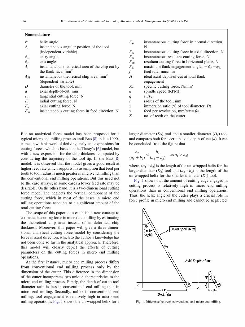
milling operations. Fig. 1 shows the un-wrapped helix for a

larger diameter (D2) tool and a smaller diameter (D1) tool

and compares both for a certain axial depth-of-cut (d). It can

be concluded from the figure that

b2

ða1 Cb2Þ!

b2

ða2 Cb2Þas a1Oa2;

where, (a1Cb2) is the length of the un-wrapped helix for the

larger diameter (D2) tool and (a2Cb2) is the length of the

un-wrapped helix for the smaller diameter (D1) tool.

Fig. 1 shows that the amount of cutting edge engaged in

cutting process is relatively high in micro end milling

operations than in conventional end milling operations.

Thus, the helix angle of the cutter plays a crucial role in

force profile in micro end milling and cannot be neglected.

M.T. Zaman et al. / International Journal of Machine Tools & Manufacture 46 (2006) 353–366 355

And because of this, a proportionately significant amount of

force is observed in the axial direction, which cannot be

overlooked. This model, therefore, provides an analytical

expression for the axial force as well making it a three-

dimensional model.

The proposed model can be used to simulate the cutting

forces accurately in a micro end milling process and can be

used effectively to monitor the tool wear. In the following

part of the paper, the developed force model is presented,

the differences between the existing models and the new

model are outlined and the simulated results are compared

with the experimental results.

Fig. 2. Schematic of the tool motions.

2. Cutting force model

This model is based on the cutting force model for

conventional end milling operations given by Tlusty and

Macneil [6] in which the tangential cutting force is assumed

to be proportional to the cutting area, which is considered as

a product of the chip thickness and the width of the chip or

the radial depth-of-cut. However, in the developed model,

the cutting area, which is nothing, but the theoretical chip

area is computed directly by considering the path of the tool

cutting edge. The assumptions of the developed model are

as follows:

Assumption 1. Instantaneous tangential component (Fti) of

the cutting force is proportional to the instantaneous

theoretical chip area (Api) [6,8]. The tangential component

of the cutting force acts in three-dimensional space in micro

end milling operation.

Fti Z KmApi; (1)

where, Km is a proportionality constant or specific force

(Pa).

Assumption 2. Instantaneous radial component (Fri) of the

cutting force is proportional to the instantaneous tangential

component (Fti) [6,8].

Fri Z qFti; (2)

where, q is proportionality constant.

Assumption 3. Instantaneous axial component (Fai) of

cutting force is the vertical component of the instantaneous

tangential force (Fti).

Fai Z Fti cosfðp=2ÞKjg (3)

where, j is the helix angle of the cutter.

Assumption 4. Machine tool dynamics, frictional and

temperature effects have been neglected and the tool is

assumed to be perfectly sharp. Since the ranges of feed per

tooth (10–20 mm) used in the current study on micro end

milling operations are comparatively higher than the cutter

edge radii (1.359 mm (for 0.5 mm dia end mill), 1.944 mm

(for a 1.0 mm dia end mill) and 2.524 mm (for a 2.0 mm dia

end mill)) of the micro end mills used, the effect of the cutter

edge radius has been neglected.

2.1. Instantaneous theoretical chip area

In the developed model, the theoretical chip area is

obtained by considering the tool work piece relative motion

and the helix of the cutter. Fig. 2 schematically shows the

cutting process in micro end milling operation. It is a two

fluted micro end milling cutter rotating in the clock-wise

direction and the direction of the feed is such that down

milling is taking place. The process has a radial depth-of-cut

(x) and an axial depth-of-cut (d). Two faces of the tool cut

the material, one is the flank face of the tool and the other is

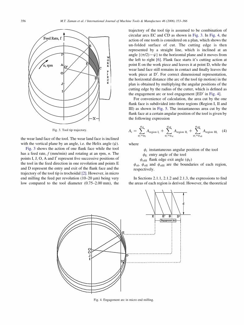
Fig. 3. Tool tip trajectory.

M.T. Zaman et al. / International Journal of Machine Tools & Manufacture 46 (2006) 353–366356

the wear land face of the tool. The wear land face is inclined

with the vertical plane by an angle, i.e. the Helix angle (j).

Fig. 3 shows the action of one flank face while the tool

has a feed rate, f (mm/min) and rotating at an rpm, n. The

points I, J, O, A and I 0 represent five successive positions of

the tool in the feed direction in one revolution and points E

and D represent the entry and exit of the flank face and the

trajectory of the tool tip is trochoidal [2]. However, in micro

end milling the feed per revolution (10–20 mm) being very

low compared to the tool diameter (0.75–2.00 mm), the

Fig. 4. Engagement arc in

trajectory of the tool tip is assumed to be combination of

circular arcs EC and CD as shown in Fig. 3. In Fig. 4, the

action of one tooth is considered on a plan, which shows the

un-folded surface of cut. The cutting edge is then

represented by a straight line, which is inclined at an

angle {(p/2)Kj} to the horizontal plane and it moves from

the left to right [6]. Flank face starts it’s cutting action at

point E on the work piece and leaves it at point D, while the

wear land face still remains in contact and finally leaves the

work piece at D 0. For correct dimensional representation,

the horizontal distance (the arc of the tool tip motion) in the

plan is obtained by multiplying the angular positions of the

cutting edge by the radius of the cutter, which is defined as

the engagement arc or tool engagement [ED 0 in Fig. 4].

For convenience of calculation, the area cut by the one

flank face is subdivided into three regions (Region I, II and

III) as shown in Fig. 5. The instantaneous area cut by the

flank face at a certain angular position of the tool is given by

the following expression

Ai ZX4oI

4iZ4E

Aregion IiC

X4oII

4iZ4oI

Aregion IIiC

X4oIII

4iZ4oII

Aregion IIIi(4)

where

fi instantaneous angular position of the tool

fE entry angle of the tool

foIII flank edge exit angle (fF)

foI, foII and foIII are the boundaries of each region,

respectively.

In Sections 2.1.1, 2.1.2 and 2.1.3, the expressions to find

the areas of each region is derived. However, the theoretical

micro end milling.

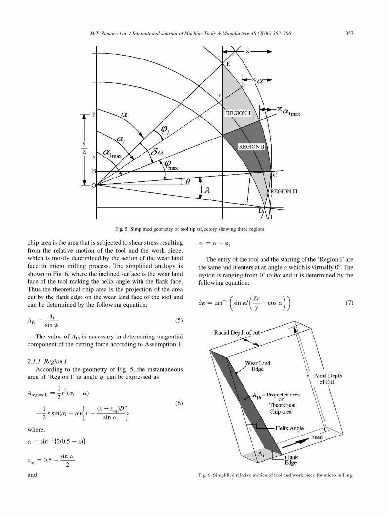
Fig. 5. Simplified geometry of tool tip trajectory showing three regions.

M.T. Zaman et al. / International Journal of Machine Tools & Manufacture 46 (2006) 353–366 357

chip area is the area that is subjected to shear stress resulting

from the relative motion of the tool and the work piece,

which is mostly determined by the action of the wear land

face in micro milling process. The simplified analogy is

shown in Fig. 6, where the inclined surface is the wear land

face of the tool making the helix angle with the flank face.

Thus the theoretical chip area is the projection of the area

cut by the flank edge on the wear land face of the tool and

can be determined by the following equation:

APi ZAi

sin j(5)

The value of APi is necessary in determining tangential

component of the cutting force according to Assumption 1.

Fig. 6. Simplified relative motion of tool and work piece for micro milling.

2.1.1. Region I

According to the geometry of Fig. 5, the instantaneous

area of ‘Region I’ at angle fi can be expressed as

Aregion IiZ

1

2r2ðai KaÞ

K1

2r sinðai KaÞ r K

ðx KxaiÞD

sin ai

� � (6)

where,

a Z sinK1f2ð0:5 KxÞg

xaiZ 0:5 K

sin ai

2

and

ai Z a C4i

The entry of the tool and the starting of the ‘Region I’ are

the same and it enters at an angle a which is virtually 08. The

region is ranging from 08 to va and it is determined by the

following equation:

va Z tanK1 sin a=Zr

yKcos a

� �� �(7)

M.T. Zaman et al. / International Journal of Machine Tools & Manufacture 46 (2006) 353–366358

Thus according to Eq. (1), ‘Region I’ ranges from fEZ00

to

4oI Z va Z tanK1 sin a. Zr

yKcos a

� �� �:

2.1.2. Region II

The expression to find instantaneous area at any position

of ‘Region II’ at any instantaneous angular position of tool

fi can be determined from Fig. 5 and can be expressed as

Aregion IIiZ

1

2r24i K

1

2r K

ðx Kx4iÞD

sinðaImaxC4iÞ

� �

!sin 4i r Kðx KxaImax

ÞD

sin aImax

� � (8)

where,

x4iZ 0:5 K

sinðaImaxC4iÞ

2;

xaImaxZ 0:5 K

sin aImax

2

and

aImaxZ a Cva Z tanK1 sin a=

Zr

yKcos a

� �� �Ca:

The ‘Region II’ ranges from 4iZaImaxZ4oI to

4i Z4max Z4oII; where, fmax can be determined from the

following equation

4max Z 90+ KsinK1 yð90+ KaÞ

180+ !D

� �Ka: (9)

2.1.3. Region III

Because of the very small dimension of this region, the

area is defined by a single quantity instead of defining it with

respect to angular displacement. The region starts at the end

of region II and extends by an angle l. From Fig. 5, the area

and the angular width of the region can be estimated from

the following equation:

AregionIII Z1

2

ffiffiffiffiffiffiffiffiffiffiffiffiffiffiffiffiffiffiffiffiffiffiffiffiffiffiffiffiffiffiffiffiffiffiffiffiffiffiffiffir2K

y

2Z cosq

� 2� �s

!y

2Z cosq

� K

ry

2Z cosq

ffiffiffiffiffiffiffiffiffiffiffiffiffiffiffiffiffiffiffiffiffiffiffiffiffiffiffiffiffiffiffiffiffir2K y

2Z cosq

� �2n or

8>><>>:9>>=>>;

(10)

and,

lZsinK1 y

ZDcosq

� (11)

where the symbols have their usual meaning.

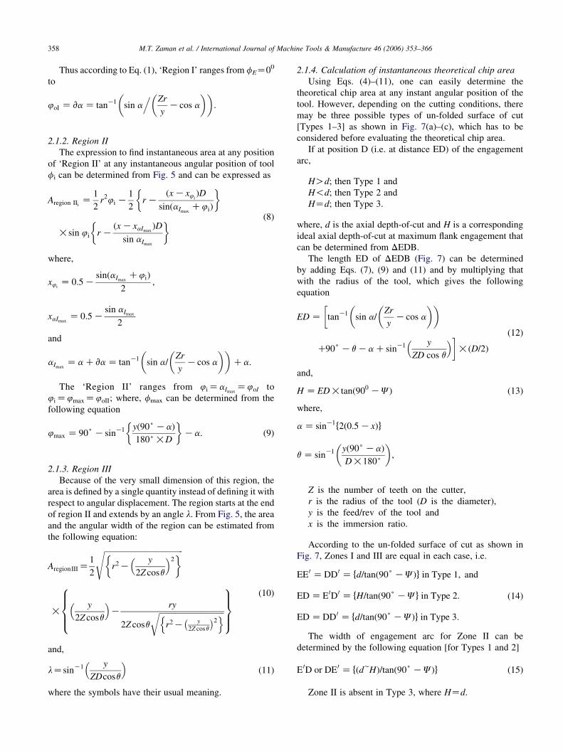
2.1.4. Calculation of instantaneous theoretical chip area

Using Eqs. (4)–(11), one can easily determine the

theoretical chip area at any instant angular position of the

tool. However, depending on the cutting conditions, there

may be three possible types of un-folded surface of cut

[Types 1–3] as shown in Fig. 7(a)–(c), which has to be

considered before evaluating the theoretical chip area.

If at position D (i.e. at distance ED) of the engagement

arc,

HOd; then Type 1 and

H!d; then Type 2 and

HZd; then Type 3.

where, d is the axial depth-of-cut and H is a corresponding

ideal axial depth-of-cut at maximum flank engagement that

can be determined from DEDB.

The length ED of DEDB (Fig. 7) can be determined

by adding Eqs. (7), (9) and (11) and by multiplying that

with the radius of the tool, which gives the following

equation

ED Z tanK1 sin a=Zr

yKcos a

� �� ��

C90+ Kq Ka CsinK1 y

ZD cos q

� �!ðD=2Þ

(12)

and,

H Z ED!tanð900 KJÞ (13)

where,

a Z sinK1f2ð0:5 KxÞg

q Z sinK1 yð90+ KaÞ

D!180+

� �;

Z is the number of teeth on the cutter,

r is the radius of the tool (D is the diameter),

y is the feed/rev of the tool and

x is the immersion ratio.

According to the un-folded surface of cut as shown in

Fig. 7, Zones I and III are equal in each case, i.e.

EE0 Z DD0 Z fd=tanð90+ KJÞg in Type 1; and

ED Z E0D0 Z fH=tanð90+ KJg in Type 2:

ED Z DD0 Z fd=tanð90+ KJÞg in Type 3:

(14)

The width of engagement arc for Zone II can be

determined by the following equation [for Types 1 and 2]

E0D or DE0 Z fðdeHÞ=tanð90+ KJÞg (15)

Zone II is absent in Type 3, where HZd.

Fig. 7. Types of uncut chip area.

M.T. Zaman et al. / International Journal of Machine Tools & Manufacture 46 (2006) 353–366 359

For both the cases the cutting process takes place from

point E to D 0. The distance ED 0 is known as engagement

angle or engagement arc.

So the total tool engagement lengths for the above three

cases will be

ED0 Z

2fd=tanð90+ KJÞgCfðH KdÞ=tanð90+ KJÞg in Type 1

2fH=tanð90+ KJÞgCfðd KHÞ=tanð90+ KJÞg in Type 2

2fd=tanð90+ KJÞg in Type 3:

8><>:(16)

2.1.4.1. Ranges of instantaneous angles and theoretical chip

areas for Type 1.

Zone 1: [fiZ0:EE 0/r]

Zone 2: [fiZEE 0/r:ED/r] and

Zone 3: [fiZED/r:ED 0/r]

Eqs. (12) and (14) can be used to determine ED and EE 0,

respectively, and ED 0 can be obtained using Eq. (16). The

way of finding the areas with angular rotation of the tool in

Zone 1 is straightforward by using (4) and (5), while the

areas of Zone 3 are similar in values to Zone 1 as they are

symmetrical. To find the area in Zone 2, the instantaneous

position of the cutter is assumed at point p as shown in

Fig. 7(a) for type 1 un-folded surface of cut. Thus

instantaneous theoretical chip area at this point can be

determined by deducting the area at angle ER/r from the

area at angle EP/r using the same set of equations, where

EP/r is the angular position of the tool and

ER=r ZðEP KPRÞ

rZ

ðEP KEE0Þ

rZ

EP

rK

EE0

r

� �as PR

Z EE0

2.1.4.2. Ranges of instantaneous angles and theoretical chip

areas for Type 2.

Zone 1: [fiZ0:ED/r]

Zone 2: [fiZED/r:EE 0/r]

Zone 3: [fiZEE 0/r:ED 0/r]

Eqs. (12) and (15) can be used to determine ED and DE 0,

respectively. Instantaneous areas of Zones 1 and 3 can easily

be determined by Eqs. (4) and (5). In this case, Zone 2 will

provide a uniform uncut chip area, thus the instantaneous

value will remain constant in this zone.

2.1.4.3. Ranges of instantaneous angles and theoretical chip

areas for Type 3.

Zone 1: [fiZ0:ED/r]

Zone 3: [fiZED/r:DD 0/r]

2.2. Cutting forces in three-dimensional co-ordinate system

The theoretical chip area can be calculated by using Eqs.

(4)–(16) and according to the assumptions, the tangential

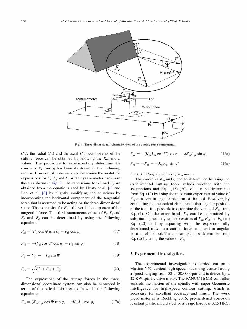
Fig. 8. Three-dimensional schematic view of the cutting force components.

M.T. Zaman et al. / International Journal of Machine Tools & Manufacture 46 (2006) 353–366360

(Ft), the radial (Fr) and the axial (Fa) components of the

cutting force can be obtained by knowing the Km and q

values. The procedure to experimentally determine the

constants Km and q has been illustrated in the following

section. However, it is necessary to determine the analytical

expressions for Fx, Fy and Fz as the dynamometer can sense

these as shown in Fig. 8. The expressions for Fx and Fy are

obtained from the equations used by Tlusty et al. [6] and

Bao et al. [8] by slightly modifying the equations by

incorporating the horizontal component of the tangential

force that is assumed to be acting on the three-dimensional

space. The expression for Fz is the vertical component of the

tangential force. Thus the instantaneous values of Fx, Fy and

Fz and Fc can be determined by using the following

equations

Fxi Z ðFti cos JÞsin 4i KFri cos 4i (17)

Fyi ZKðFti cos JÞcos 4i KFri sin 4i (18)

Fzi Z Fai ZKFti sin J (19)

Fci ZffiffiffiffiffiffiffiffiffiffiffiffiffiffiffiffiffiffiffiffiffiffiffiffiffiffiffiffiffiF2

xi CF2yi CF2

zi

q(20)

The expressions of the cutting forces in the three-

dimensional coordinate system can also be expressed in

terms of theoretical chip area as shown in the following

equations:

Fxi Z ðKmApi cos JÞsin 4i KqKmApi cos 4i (17a)

Fyi ZKðKmApi cos JÞcos 4i KqKmApi sin 4i (18a)

Fzi ZKFai ZKKmApi sin J (19a)

2.2.1. Finding the values of Km and q

The constants Km and q can be determined by using the

experimental cutting force values together with the

assumptions and Eqs. (17)–(20). Fti can be determined

from Eq. (19) by using the maximum experimental value of

Fzi at a certain angular position of the tool. However, by

computing the theoretical chip area at that angular position

of the tool, it is possible to determine the value of Km from

Eq. (1). On the other hand, Fri can be determined by

substituting the analytical expressions of Fxi, Fyi and Fzi into

Eq. (20) and by equating with the experimentally

determined maximum cutting force at a certain angular

position of the tool. The constant q can be determined from

Eq. (2) by using the value of Fri.

3. Experimental investigations

The experimental investigation is carried out on a

Makino V55 vertical high-speed machining center having

a speed ranging from 50 to 30,000 rpm and is driven by a

22 KW spindle drive motor. The FANUC 16 MB controller

controls the motion of the spindle with super Geometric

Intelligence for high-speed contour cutting, which is

necessary for excellent accuracy and finish. The work

piece material is Rochling 2316, pre-hardened corrosion

resistant plastic mould steel of average hardness 32.5 HRC,

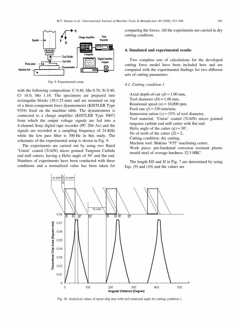
Fig. 9. Experimental setup.

M.T. Zaman et al. / International Journal of Machine Tools & Manufacture 46 (2006) 353–366 361

with the following composition: C 0.40, Mn 0.70, Si 0.40,

Cr 16.0, Mo 1.10. The specimens are prepared into

rectangular blocks (30!25 mm) and are mounted on top

of a three-component force dynamometer (KISTLER Type

9354) fixed on the machine table. The dynamometer is

connected to a charge amplifier (KISTLER Type 5007)

from which the output voltage signals are fed into a

4-channel Sony digital tape recorder (PC 204 Ax) and the

signals are recorded at a sampling frequency of 24 KHz

while the low pass filter is 300 Hz in this study. The

schematic of the experimental setup is shown in Fig. 9.

The experiments are carried out by using two fluted

‘Union’ coated (TiAlN) micro grained Tungsten Carbide

end mill cutters, having a Helix angle of 308 and flat end.

Numbers of experiments have been conducted with these

conditions and a normalized value has been taken for

Fig. 10. Analytical values of uncut chip area with

comparing the forces. All the experiments are carried in dry

cutting condition.

4. Simulated and experimental results

Two complete sets of calculations for the developed

cutting force model have been included here and are

compared with the experimental findings for two different

sets of cutting parameters.

4.1. Cutting condition 1

Axial depth-of-cut (d)Z1.00 mm,

Tool diameter (D)Z1.00 mm,

Rotational speed (n)Z10,000 rpm,

Feed rate (f)Z150 mm/min,

Immersion ration (x)Z15% of tool diameter,

Tool material: ‘Union’ coated (TiAlN) micro grained

tungsten carbide end mill cutter with flat end.

Helix angle of the cutter (j)Z308,

No of teeth of the cutter (Z)Z2,

Cutting condition: dry cutting,

Machine tool: Makino ‘V55’ machining center,

Work piece: pre-hardened corrosion resistant plastic

mould steel of average hardness 32.5 HRC.

The length ED and H in Fig. 7 are determined by using

Eqs. (9) and (10) and the values are

tool rotational angle for cutting condition 1.

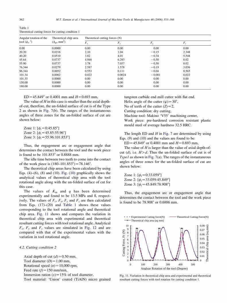
Table 1

Theoretical cutting forces for cutting condition 1

Angular rotation of the

tool (fi, 8)

Theoretical chip area

(Api, mm2)

Theoretical cutting forces (N)

Fx Fy Fz Fc

0.00 0.0000 0.00 0.00 0.00 0.00

20.20 0.0216 2.10 1.04 K0.15 2.348

40.20 0.0510 3.82 4.01 K0.34 5.548

45.64 0.0737 4.948 6.293 K0.50 8.02

55.90 0.0737 3.78 7.057 K0.50 8.02

76.344 0.0279 2.587 1.578 K0.19 3.036

96.344 0.0052 0.553 0.111 K0.04 0.565

101.34 0.0002 0.022 0.0024 K0.001 0.022

101.55 0.0000 0.00 0.00 0.00 0.00

150.00 0.0000 0.00 0.00 0.00 0.00

180.00 0.0000 0.00 0.00 0.00 0.00

789

10

, Fc

(N)

0.05

0.06

0.07

0.08

rea

(sq.

mm

)

Experimental Cutting force(N) Theoretical Cutting Force(N)Theoretical chip area (sq mm)

M.T. Zaman et al. / International Journal of Machine Tools & Manufacture 46 (2006) 353–366362

EDZ45.8498 or 0.4001 mm and HZ0.693 mm,

The value of H in this case is smaller than the axial depth-

of-cut, therefore, the un-folded surface of cut is of the Type

2 as shown in Fig. 7(b). The ranges of the instantaneous

angles of three zones for the un-folded surface of cut are

shown below:

Zone 1: [fiZ0:45.858]

Zone 2: [fiZ45.85:55.968]

Zone 3: [fiZ55.96:101.8538]

Thus, the engagement arc or engagement angle that

determines the contact between the tool and the work piece

is found to be 101.8538 or 0.8888 mm.

The idle time between two teeth to come into the contact

of the work piece is (180–101.8538)Z78.1468.

The theoretical chip areas have been calculated by using

Eqs. (4)–(6), (8) and (10). Fig. (10) graphically shows the

analytical values of theoretical chip area with the tool

rotational angle along with the un-folded surface of cut for

this case.

The values of Km and q has been determined

experimentally and found to be 13.5 MPa and 8, respect-

ively. The values of Fc, Fx, Fy and Fz are then calculated

from Eqs. (17)–(20) and Table 1 shows these values

corresponding to the tool rotational angle and theoretical

chip area. Fig. 11 shows and compares the variation in

theoretical chip area with experimental and theoretical

resultant cutting forces with tool rotational angle. Analytical

Fx, Fy and Fz values are simulated in Fig. 12 and are

compared with that of the experimental values with the

variation in tool rotational angle.

0123456

0 100 200 300 400 500

Angluar Rotation of the tool (Degree)

Cut

ting

Forc

e

0

0.01

0.02

0.03

0.04

The

oret

ical

chi

p a

Fig. 11. Variation in theoretical chip area and experimental and theoretical

resultant cutting forces with tool rotation for cutting condition 1.

4.2. Cutting condition 2

Axial depth-of-cut (d)Z0.50 mm,

Tool diameter (D)Z1.00 mm,

Rotational speed (n)Z10,000 rpm,

Feed rate (f)Z150 mm/min,

Immersion ration (x)Z15% of tool diameter,

Tool material: ‘Union’ coated (TiAlN) micro grained

tungsten carbide end mill cutter with flat end.

Helix angle of the cutter (j)Z308,

No of teeth of the cutter (Z)Z2,

Cutting condition: dry cutting,

Machine tool: Makino ‘V55’ machining center,

Work piece: pre-hardened corrosion resistant plastic

mould steel of average hardness 32.5 HRC.

The length ED and H in Fig. 7 are determined by using

Eqs. (9) and (10) and the values are found to be:

EDZ45.8498 or 0.4001 mm and HZ0.693 mm,

The value of H is larger than the value of axial depth-of-

cut (d), i.e. HOd. Thus the un-folded surface of cut is of

Type1 as shown in Fig. 7(a). The ranges of the instantaneous

angles of three zones for the un-folded surface of cut are

shown below:

Zone 1: [fiZ0:33.0598]

Zone 2: [fiZ33.059:45.8498]

Zone 3: [fiZ45.849:78.9088]

Thus, the engagement arc or engagement angle that

determines the contact between the tool and the work piece

is found to be 78.9088 or 0.6886 mm.

-1

0

1

2

3

4

5

6

7

8

9

0 100 200 300 400 500

Angular rotation of the tool (deg)

Forc

e (N

)

Fx-Experimental Fy-Experimental Fz-ExperimentalFx-Theoretical Fy-Theoretical Fz-Theoretical

Fig. 12. Comparison between experimental and theoretical cutting forces

for cutting condition 1.

M.T. Zaman et al. / International Journal of Machine Tools & Manufacture 46 (2006) 353–366 363

The idle time between two teeth to come into the contact

of the work piece is (180–78.9088)Z101.0928.

The theoretical chip areas have been calculated by using

Eqs. (4)–(6), (8) and (10). Fig. 13 graphically shows the

analytical values of theoretical chip area with the tool

rotational angle along with the un-folded surface of cut for

this case.

The values of Km and q are 13.5 and 8 MPa, respectively,

and the values of Fc, Fx, Fy and Fz are calculated from Eqs.

(17)–(20) and are shown in Table 2. Fig. 14 shows and

compares the variation in theoretical chip area with

experimental and theoretical resultant cutting forces with

tool rotation angle. Analytical Fx, Fy and Fz values are

simulated in Fig. 15 and are compared with that of

Fig. 13. Analytical values of uncut chip area with

the experimental values with the variation in tool rotational

angle.

5. Estimation of tool-wear in micro end milling

A thorough study on the behavior of tool life with

changes in cutting conditions has been done while

performing the experiments. Premature tool failures at

very low depths of cut are frequently observed in micro end

milling operations and unlike in conventional end milling

operations, tool life increases in micro end milling

operations with increase in axial depth-of-cut to a certain

extent [9,10].

Fig. 16 shows the flank-wear propagation with cutting

time in 1.00 mm diameter tool at varying axial depths of cut.

Once the flank wear starts increasing exponentially with

time, the tool is considered ‘failed’ or if catastrophic failure

is diagnosed then the tool is considered ‘failed’. Thus the

tool life for 1.00 mm tool is calculated at various depths of

cut are given in Table 3 and Fig. 17 it is clear that tool life is

increasing within this range of axial depths of cut. This

behavior of tool life in micro end milling is opposite to that

in conventional end milling operations, where the tool life

decreases with an increase in axial depth-of-cut.

This ambiguous behavior of micro end milling process is

due to the relatively higher tool engagement of the micro

end mill cutter with the work piece than the conventional

end mill cutter for a certain set of cutting parameters and

this engagement increases with the increase in axial depth-

of-cut. Eq. (16) gives the analytical expressions to

determine the tool engagement length or the angles for

end mill cutters. The engagement angle values for 1.00 mm

tool rotational angle for cutting condition 2.

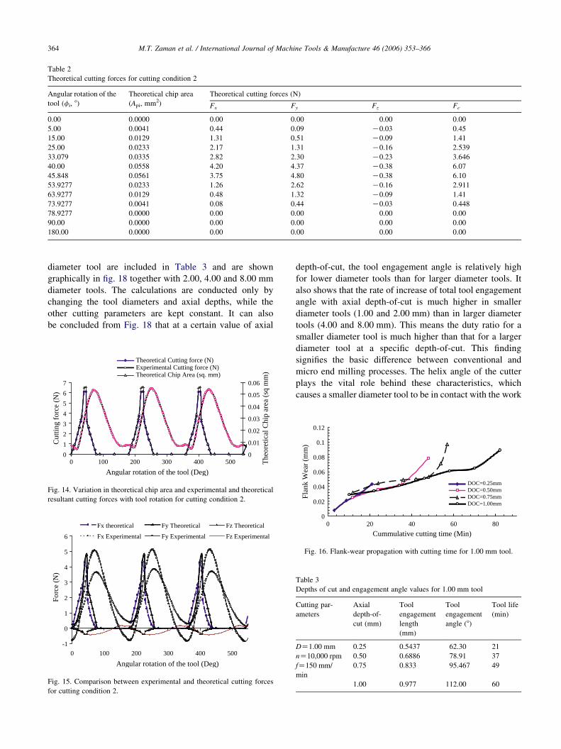
Table 2

Theoretical cutting forces for cutting condition 2

Angular rotation of the

tool (fi, 8)

Theoretical chip area

(Api, mm2)

Theoretical cutting forces (N)

Fx Fy Fz Fc

0.00 0.0000 0.00 0.00 0.00 0.00

5.00 0.0041 0.44 0.09 K0.03 0.45

15.00 0.0129 1.31 0.51 K0.09 1.41

25.00 0.0233 2.17 1.31 K0.16 2.539

33.079 0.0335 2.82 2.30 K0.23 3.646

40.00 0.0558 4.20 4.37 K0.38 6.07

45.848 0.0561 3.75 4.80 K0.38 6.10

53.9277 0.0233 1.26 2.62 K0.16 2.911

63.9277 0.0129 0.48 1.32 K0.09 1.41

73.9277 0.0041 0.08 0.44 K0.03 0.448

78.9277 0.0000 0.00 0.00 0.00 0.00

90.00 0.0000 0.00 0.00 0.00 0.00

180.00 0.0000 0.00 0.00 0.00 0.00

M.T. Zaman et al. / International Journal of Machine Tools & Manufacture 46 (2006) 353–366364

diameter tool are included in Table 3 and are shown

graphically in fig. 18 together with 2.00, 4.00 and 8.00 mm

diameter tools. The calculations are conducted only by

changing the tool diameters and axial depths, while the

other cutting parameters are kept constant. It can also

be concluded from Fig. 18 that at a certain value of axial

0

1

2

3

4

5

6

7

0 100 200 300 400 500

Angular rotation of the tool (Deg)

Cut

ting

forc

e (N

)

0

0.01

0.02

0.03

0.04

0.05

0.06

The

oret

ical

Chi

p ar

ea (

sq m

m)

Theoretical Cutting force (N)Experimental Cutting force (N)Theoretical Chip Area (sq. mm)

Fig. 14. Variation in theoretical chip area and experimental and theoretical

resultant cutting forces with tool rotation for cutting condition 2.

-1

0

1

2

3

4

5

6

0 100 200 300 400 500

Angular rotation of the tool (Deg)

Forc

e (N

)

Fx theoretical Fy Theoretical Fz Theoretical

Fx Experimental Fy Experimental Fz Experimental

Fig. 15. Comparison between experimental and theoretical cutting forces

for cutting condition 2.

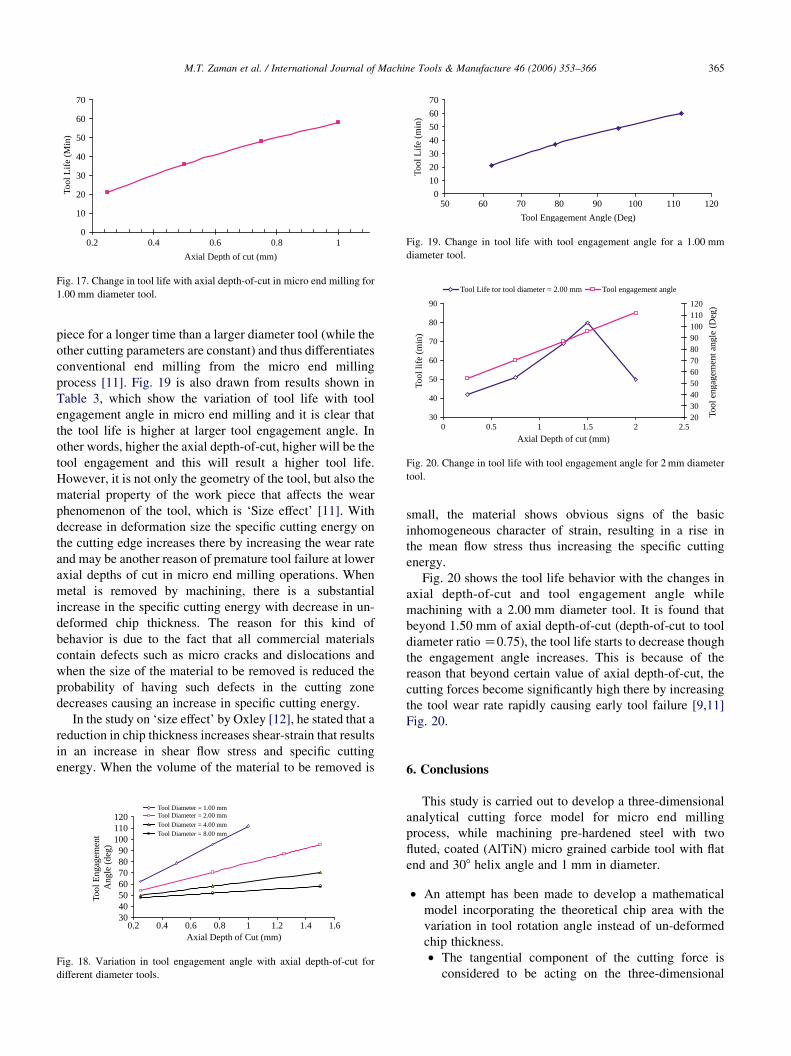
depth-of-cut, the tool engagement angle is relatively high

for lower diameter tools than for larger diameter tools. It

also shows that the rate of increase of total tool engagement

angle with axial depth-of-cut is much higher in smaller

diameter tools (1.00 and 2.00 mm) than in larger diameter

tools (4.00 and 8.00 mm). This means the duty ratio for a

smaller diameter tool is much higher than that for a larger

diameter tool at a specific depth-of-cut. This finding

signifies the basic difference between conventional and

micro end milling processes. The helix angle of the cutter

plays the vital role behind these characteristics, which

causes a smaller diameter tool to be in contact with the work

Table 3

Depths of cut and engagement angle values for 1.00 mm tool

Cutting par-

ameters

Axial

depth-of-

cut (mm)

Tool

engagement

length

(mm)

Tool

engagement

angle (8)

Tool life

(min)

DZ1.00 mm 0.25 0.5437 62.30 21

nZ10,000 rpm 0.50 0.6886 78.91 37

fZ150 mm/

min

0.75 0.833 95.467 49

1.00 0.977 112.00 60

0

0.02

0.04

0.06

0.08

0.1

0.12

0 20 40 60 80

Cummulative cutting time (Min)

Flan

k W

ear

(mm

)

DOC=0.25mmDOC=0.50mmDOC=0.75mmDOC=1.00mm

Fig. 16. Flank-wear propagation with cutting time for 1.00 mm tool.

0

10

20

30

40

50

60

70

50 60 70 80 90 100 110 120

Tool Engagement Angle (Deg)

Tool

Lif

e (m

in)

Fig. 19. Change in tool life with tool engagement angle for a 1.00 mm

diameter tool.

0

10

20

30

40

50

60

70

0.2 0.4 0.6 0.8 1

Axial Depth of cut (mm)

Tool

Lif

e (M

in)

Fig. 17. Change in tool life with axial depth-of-cut in micro end milling for

1.00 mm diameter tool.

30

40

50

60

70

80

90

0 0.5 1 1.5 2 2.5

Axial Depth of cut (mm)

Tool

life

(m

in)

2030405060708090100110120

Tool

eng

agem

ent a

ngle

(D

eg)

Tool Life tor tool diameter = 2.00 mm Tool engagement angle

Fig. 20. Change in tool life with tool engagement angle for 2 mm diameter

tool.

M.T. Zaman et al. / International Journal of Machine Tools & Manufacture 46 (2006) 353–366 365

piece for a longer time than a larger diameter tool (while the

other cutting parameters are constant) and thus differentiates

conventional end milling from the micro end milling

process [11]. Fig. 19 is also drawn from results shown in

Table 3, which show the variation of tool life with tool

engagement angle in micro end milling and it is clear that

the tool life is higher at larger tool engagement angle. In

other words, higher the axial depth-of-cut, higher will be the

tool engagement and this will result a higher tool life.

However, it is not only the geometry of the tool, but also the

material property of the work piece that affects the wear

phenomenon of the tool, which is ‘Size effect’ [11]. With

decrease in deformation size the specific cutting energy on

the cutting edge increases there by increasing the wear rate

and may be another reason of premature tool failure at lower

axial depths of cut in micro end milling operations. When

metal is removed by machining, there is a substantial

increase in the specific cutting energy with decrease in un-

deformed chip thickness. The reason for this kind of

behavior is due to the fact that all commercial materials

contain defects such as micro cracks and dislocations and

when the size of the material to be removed is reduced the

probability of having such defects in the cutting zone

decreases causing an increase in specific cutting energy.

In the study on ‘size effect’ by Oxley [12], he stated that a

reduction in chip thickness increases shear-strain that results

in an increase in shear flow stress and specific cutting

energy. When the volume of the material to be removed is

30405060708090

100110120

0.2 0.4 0.6 0.8 1 1.2 1.4 1.6Axial Depth of Cut (mm)

Tool

Eng

agem

ent

Ang

le (

deg)

Tool Diameter = 1.00 mmTool Diameter = 2.00 mmTool Diameter = 4.00 mmTool Diameter = 8.00 mm

Fig. 18. Variation in tool engagement angle with axial depth-of-cut for

different diameter tools.

small, the material shows obvious signs of the basic

inhomogeneous character of strain, resulting in a rise in

the mean flow stress thus increasing the specific cutting

energy.

Fig. 20 shows the tool life behavior with the changes in

axial depth-of-cut and tool engagement angle while

machining with a 2.00 mm diameter tool. It is found that

beyond 1.50 mm of axial depth-of-cut (depth-of-cut to tool

diameter ratio Z0.75), the tool life starts to decrease though

the engagement angle increases. This is because of the

reason that beyond certain value of axial depth-of-cut, the

cutting forces become significantly high there by increasing

the tool wear rate rapidly causing early tool failure [9,11]

Fig. 20.

6. Conclusions

This study is carried out to develop a three-dimensional

analytical cutting force model for micro end milling

process, while machining pre-hardened steel with two

fluted, coated (AlTiN) micro grained carbide tool with flat

end and 308 helix angle and 1 mm in diameter.

† An attempt has been made to develop a mathematical

model incorporating the theoretical chip area with the

variation in tool rotation angle instead of un-deformed

chip thickness.

† The tangential component of the cutting force is

considered to be acting on the three-dimensional

M.T. Zaman et al. / International Journal of Machine Tools & Manufacture 46 (2006) 353–366366

space because of the higher depth-of-cut to tool

diameter ratio in micro end milling and that leads to a

significant amount of cutting force in axial direction.

The maximum values of the cutting forces are found

to be almost equal to the experimental values.

† The developed model can be used to simulate the

cutting forces accurately to 90% average accuracy.

References

[1] L. Zheng, Y.S. Chiou, S.Y. Liang, Three dimensional cutting force

analysis in end milling, IJMS 38 (3) (1996) 259–269.

[2] M.E. Martellotti, An analysis of the milling process, Transaction of

ASME 63 (1941) 677–700.

[3] A.J.P. Sabberwal, Chip Section and cutting force during the milling

operation, CIRP Annals 10 (3) (1961) 62.

[4] W.A. Kline, R.E. DeVor, J.R. Lindberg, The prediction of cutting

forces in end milling with application to concerning cuts, IJMTDR 22

(1) (1982) 7–22.

[5] G. Yucesan, Y. Altintas, Improved modeling of cutting force

coefficients in peripheral milling, International Journal of Machine

Tools and Manufacture 4 (4) (1993) 473–487.

[6] J. Tlusty, P. Macneil, Dynamics of cutting forces in end milling,

Annals of CIRP 24 (1) (1975) 21–25.

[7] I. Yellowley, Observations on the mean values of the forces, torque

and specific power in the peripheral milling process, International

Journal of Machine Tool Manufactures Design and Research 25 (4)

(1985) 337–346.

[8] W.Y. Bao, I. Tansel, Modeling micro end milling operations, Part I:

analytical cutting force model, International Journal of Machine Tool

and Manufacture 40 (2000) 2155–2173.

[9] M.Tauhiduzzaman, M. Rahman, A. Senthil Kumar, S. Sreeram, Effect

of engagement arc on tool life in micro end milling. Third

International Conference on Advanced Manufacturing Technology,

2004, Kuala Lumpur, Malaysia, 49–54.

[10] M. Rahman, A. Senthil Kumar, J.R.S. Prakash, Micro milling of pure

copper, Journal of Material Processing technology 116 (1) (2001) 39–

43.

[11] M.T. Zaman, A. Senthil Kumar, M. Rahman, H.S. Lim, S. Sreeram,

Tool wear in micro end milling operation: influence of tool

engagement and size effect, International Journal of Machine Tool

and Manufacture, (In Review).

[12] P.L.B. Oxley, Mechanics of Machining: An Analytical Approach to

Assessing Machinability, Ellis Horwood Series, 1989.