YNAMIC - Columbia Business School · in scop e and in qualit y, ... Lab oratory. In teracting with Mik ... applications in these div erse domains, the mathematical theory of \sto

$Page 1: YNAMIC - Columbia Business School · in scop e and in qualit y, ... Lab oratory. In teracting with Mik ... applications in these div erse domains, the mathematical theory of \sto$
DYNAMIC CONTROL OF STOCHASTIC PROCESSING

NETWORKS: A FLUID MODEL APPROACH

A DISSERTATION

SUBMITTED TO THE DEPARTMENT OF ELECTRICAL ENGINEERING

AND THE COMMITTEE ON GRADUATE STUDIES

OF STANFORD UNIVERSITY

IN PARTIAL FULFILLMENT OF THE REQUIREMENTS

FOR THE DEGREE OF

DOCTOR OF PHILOSOPHY

Constantinos Maglaras

August 1998

c Copyright 1998 by Constantinos Maglaras

All Rights Reserved

ii

I certify that I have read this thesis and that in my opinion it is fully adequate,

in scope and in quality, as a dissertation for the degree of Doctor of Philosophy.

Sunil Kumar (Principal Adviser)



Stephen Boyd



J. Michael Harrison



Nicholas Bambos

Approved for the University Committee on Graduate Studies:

iii

iv

Abstract

Today's communication, computer and manufacturing industries o�er many examples

of technological systems in which \units of work" visit a number of di�erent \servers"

in the course of their processing, and in which the work ow is subject to stochastic

variability. Our work focuses on dynamic control for these \stochastic processing

networks."

In general, stochastic processing networks are di�cult to analyze and control, and,

with very few exceptions, problems of realistic scale quickly become analytically and

computationally intractable. One promising approach in addressing these problems

that has emerged from research over the past 10-15 years, uses a hierarchy of approxi-

mate models that provide tractable \relaxations" of the original problem as the basis

for analysis and synthesis of \good" control policies. In particular, the analytical

theory associated with uid approximations and with Brownian approximations has

produced important insights in understanding how the performance of a multiclass

network depends on di�erent design and control parameters.

The work in this dissertation follows along the same lines. Speci�cally, the ap-

proach taken here is based on approximating (or replacing) the stochastic network

by its uid analog, this is a model with deterministic and continuous dynamics, solv-

ing an associated uid optimal control problem, and then using the derived uid

control policy in order to de�ne an implementable policy in the original stochastic

network. A major obstacle in this policy design methodology is in translating the

v

vi ABSTRACT

information derived from analysis of the tractable approximate model into an im-

plementable policy in the stochastic system in a way that guarantees stability and

optimal or \near-optimal" performance. This problem has been recognized by many

researchers in relation to both uid and Brownian (di�usion) approximations in the

past. The main contribution of this thesis will be in proposing and analyzing a family

of discrete-review policies that addresses and solves this problem. Each policy in this

family translates the solution of an associated uid optimal control problem in an

implementable policy for the stochastic network, in a way that guarantees stability

and achieves asymptotically optimal performance under uid scaling.

Thereafter, several extensions to this framework are presented. First, the family

of uid control policies is greatly generalized to allow arbitrary trajectory tracking

policies as well as a general family of greedy control laws motivated by the solution

of the uid optimal control problems studied above. Second, the class of networks

under consideration is extended in order to allow routing and input (or admission)

control capability, as well as other features often excluded from mainstream queueing

theory, such as multi-server or batch-processing stations, and setup (or switchover)

times.

Acknowledgements

Through the course of my studies I have had the great fortune to get to know and

interact with my three academic advisors, Professors Boyd, Harrison, and Kumar.

Their talent, diverse backgrounds, interests, and teaching and research styles have

provided for me an exceptional opportunity to learn that has shaped me as a scholar

and a person. I am indebted to all three.

I am grateful to Professor Stephen Boyd for his constant support and encourage-

ment. His talent, broad interests, and his intellectual curiosity and intensity, have

always served as a source of motivation. My �rst introduction to the subject matter

of this thesis (as well as many other things) came from Professor Michael Harrison.

His continuing guidance and profound enthusiasm have been a catalyst for this work.

Our close interaction has greatly in uenced me and has triggered in part the career

shift that I am about to undertake. Finally, I have been fortunate to have Professor

Sunil Kumar serve as my principal advisor. In his two years at Stanford, he has

provided invaluable support and help that have signi�cantly impacted my academic

life and future career choices.

I would also like to thank Professor Nicholas Bambos for serving in my committees

and, more importantly, for his friendship and support.

My association with Stanford Integrated Manufacturing Association (SIMA) and

my participation to the FPM Ph.D. Program has been a rewarding experience that

has broaden my horizons. I am grateful for their generous support { both �nancial

vii

viii ACKNOWLEDGEMENTS

and educational. I also need to thank my fellow students in the Information Systems

Laboratory. Interacting with Mike Grant, Haitham Hindi, Shao-Po Wu, Arrash Has-

sibi, Miguel Lobo, Maryam Fazel, Cesar Crusius, Yiannis Kontoyiannis, Bijit Halder,

Suhas Degavi, Assaf Zeevi, as well as my FPM classmates has been and educational

and rewarding experience. The last few years have been enriched by Niki's loving

support, (endurance) and friendship.

Finally, I want to express my deepest appreciation for my grandfather Constanti-

nos, my parents Dimos and Chrysoula, my sister Marianna, and my brother Alexan-

dros for being a constant source of loving support and encouragement throughout the

years. It is to them that I dedicate this thesis.

Contents

Abstract v

Acknowledgements vii

1 Introduction 1

1.1 An illustrative example . . . . . . . . . . . . . . . . . . . . . . . . . . 5

1.2 The uid model approach . . . . . . . . . . . . . . . . . . . . . . . . 14

1.3 Thesis outline . . . . . . . . . . . . . . . . . . . . . . . . . . . . . . . 19

2 Network models 21

2.1 Multiclass open queueing network models . . . . . . . . . . . . . . . . 22

2.2 Fluid models . . . . . . . . . . . . . . . . . . . . . . . . . . . . . . . 27

2.3 Stability . . . . . . . . . . . . . . . . . . . . . . . . . . . . . . . . . . 30

2.4 Fluid optimal control problems . . . . . . . . . . . . . . . . . . . . . 34

2.4.1 Characterization of optimal control policies . . . . . . . . . . . 35

2.4.2 Algorithms for uid optimal control problems . . . . . . . . . 41

2.5 Fluid-scale asymptotic optimality . . . . . . . . . . . . . . . . . . . . 43

3 Asymptotic optimality via discrete-review policies 47

3.1 Speci�cation of a discrete-review policy . . . . . . . . . . . . . . . . . 48

3.2 The uid model associated with DR(rg; l; �) . . . . . . . . . . . . . . 56

ix

x CONTENTS

3.2.1 Preliminaries: Large deviations bounds . . . . . . . . . . . . . 57

3.2.2 Derivation of the associated uid models . . . . . . . . . . . . 60

3.3 Asymptotic optimality of DR(rg; l; �) . . . . . . . . . . . . . . . . . . 67

4 Trajectory tracking via discrete-review policies 71

4.1 Policy description . . . . . . . . . . . . . . . . . . . . . . . . . . . . . 72

4.1.1 Preliminaries . . . . . . . . . . . . . . . . . . . . . . . . . . . 72

4.1.2 Speci�cation of DR(; l; �) . . . . . . . . . . . . . . . . . . . 74

4.2 The uid model associated with DR(; l; �) . . . . . . . . . . . . . . 75

4.3 Examples of trajectory tracking policies . . . . . . . . . . . . . . . . . 79

5 Extensions 87

5.1 Greedy uid control policies . . . . . . . . . . . . . . . . . . . . . . . 87

5.1.1 Stability of greedy policies . . . . . . . . . . . . . . . . . . . . 90

5.1.2 Examples of greedy control policies . . . . . . . . . . . . . . . 94

5.2 A more general class of network models . . . . . . . . . . . . . . . . . 96

5.2.1 Adding more control capability . . . . . . . . . . . . . . . . . 97

5.2.2 Closed multiclass queueing networks . . . . . . . . . . . . . . 102

5.2.3 Server characteristics . . . . . . . . . . . . . . . . . . . . . . . 104

6 Concluding remarks 107

A Some additional proofs 113

A.1 Large deviation bounds for DR(rg; l; �) . . . . . . . . . . . . . . . . . 113

A.2Discrete-review policies with zero safety stocks . . . . . . . . . . . . . . 118

B Nomenclature 125

Bibliography 129

List of Figures

1.1 Typical route of a wafer type through a semiconductor fab . . . . . . 3

1.2 The Rybko-Stolyar network . . . . . . . . . . . . . . . . . . . . . . . 6

1.3 Optimal state trajectories in the uid model for z = [1; 0; 0:5; 1] . . . 10

1.4 State trajectories under LBFS/PR: Q(0) = 400[1; 0; 0:5; 1]; n = 400 . 10

1.5 Policy design procedure via uid models . . . . . . . . . . . . . . . . 15

3.1 Algorithmic description of DR(rg; l; �) . . . . . . . . . . . . . . . . . 52

3.2 State evolution under a discrete-review policy . . . . . . . . . . . . . 53

3.3 Discrete-review policy: a schematic representation . . . . . . . . . . . 58

4.1 Optimal uid trajectories (vs) state trajectories underCR(g; �): Q(0) =

200[1; 0; 0:5; 1]; (n = 200) . . . . . . . . . . . . . . . . . . . . . . . . . 81

xi

xii LIST OF FIGURES

Chapter 1

Introduction

Today's communication, computer and manufacturing industries o�er many examples

of technological systems in which \units of work" visit a number of di�erent \servers"

in the course of their processing, and in which the work ow is subject to stochastic

variability. Motivated by applications in these diverse domains, the mathematical

theory of \stochastic processing networks" has developed rapidly as a research area

in recent decades.

A general formulation of stochastic processing networks was proposed by Harri-

son in [54] and it can be described in these terms: �rst, there are di�erent types of

jobs, customers, or other units of ow in the system; second, there are tasks to be

performed for each type of job; and �nally, there are processing resources of �nite

capacity that are required in performing these tasks. Control in these networks in-

volves resource allocation decisions, routing decisions and input control (or admission

control) decisions. Mathematical models of stochastic processing networks include

classical queueing network models, such as product form networks analyzed in the

pioneering work of Jackson [62,63], Baskett, Chandy, Muntz and Palacios [8] and

Kelly [67], and the more general family of multiclass queueing networks described

by Harrison in [52], which has been a topic of intense research over the past decade.

1

2 CHAPTER 1. INTRODUCTION

Also, included are models with features excluded from mainstream queueing theory,

such as simultaneous resource requirements.

In general, stochastic processing networks are di�cult to analyze and control,

and, with very few exceptions, problems of realistic scale quickly become analytically

and computationally intractable. This is due to three characteristic features of these

systems that contribute to their overall complexity: ows are discrete, system dynam-

ics are crucial, and stochastic variability plays a central role. Due to the inherent

complexity of these systems, no general theory has been developed to this point and

despite the extensive literature of the �eld, theoretical and practical developments

are segmented according to their target application.

The main focus of this thesis will be in designing dynamic control policies for

stochastic processing networks motivated by modern manufacturing systems, which

might include any one of the three elements of control mentioned above, or combi-

nations thereof, in order to guarantee stability and/or optimize some performance

criterion of interest. Network control problems tend to have distinctly di�erent char-

acteristics in di�erent application domains. For example, while in communication

networks the state descriptor has dimension of the order of millions, or even billions,

and the \thinking" times between decisions is of the order of tens of nanoseconds,

in manufacturing systems state descriptors may have dimension in the hundreds and

allowed \thinking" time in the order of seconds, or even minutes.

Typically, when a complex manufacturing system is represented as a stochastic

processing network, one sees many workstations at which jobs are processed, usually

one at a time. There may be multiple types of jobs owing through the network and

each job type may have its own processing requirements at each station. Stochastic

variability is a result of variable processing times, external demand variability, server

unreliability, yield variability, or any number of other sources. For example, a sim-

pli�ed model of a semiconductor fabrication plant depicting the actual route of one

3

1 4

7

11

12

13

14

15 17

24

ENTER

IMPLANT

ALIGN

FURNACE

20/21

8/9

5/62

10

18/19 22/23

16

3

Figure 1.1: Typical route of a wafer type through a semiconductor fab


wafer type through the fab is shown in Figure 1.1. Only three primary bottleneck sta-

tions are drawn here, namely furnace, align, and implant; the fab actually produces

several di�erent types of wafers and there are 19 stations in total. The total number

of type-step combinations, called job classes, is around 1000 in total, although only

24 of them are drawn in the �gure. Di�erent steps of processing of the same type

of wafer in the same station may have di�erent service requirements, and there is a

many-to-one relation between job classes and stations. The controller has discretion

as to the sequencing of jobs of the various classes at each workstation, and at any

point in time, full information regarding the state of the network is available towards

making these decisions.

Such systems are accurately modeled as multiclass queueing networks [120,82,117],

while several other applications are described in the general references in [48,16,26].

The mathematical model of a multiclass queueing network, in the form that it is re-

ferred to here, was �rst described by Harrison in [52]. The probabilistic assumptions

imposed are that general distributions are allowed but all processes should jointly

satisfy a functional law of large numbers; these are the necessary assumptions for the

analysis that follows. Centralized dynamic control policies with sequencing, routing,

and admission control capabilities are considered, where it is assumed that the con-

troller has complete information regarding the state of the network at any decision

instant. This class of mathematical models has been studied extensively over the past

decade and will also serve as the basic network models in this thesis. This will help

anchor ideas and relate the proposed methodology to the powerful tools developed so

far in the literature.

Prior to proceeding with a detailed discussion of the class of problems of interest

here, it is appropriate to add some remarks regarding the relevant literature in the

�eld. Speci�cally, we provide two pointers towards two di�erent sets of references

that lie within the general subject matter of this thesis, but are not closely related

1.1. AN ILLUSTRATIVE EXAMPLE 5

to the work presented here and will not be pursued any further. The �rst is in the

context of deterministic scheduling problems that has originated from the �elds of

operations research and computer networks. A comprehensive review article (with

many references therein) is the article by Lawler, Lenstra, Rinnooy Kan and Shmoys

[80]. The results is this �eld focus more on the combinatorial nature of these problems,

their computational complexity, as well as approximation algorithms for some classes

of problems. The second is in the context of communication networks, where the focus

is in large distributed systems where one normally imposes fewer assumptions on the

speci�c network structure, the probabilistic environment, or the information available

to the controllers in making their various decisions. This should be contrasted with

the assumptions regarding probabilistic structure and the full state information of the

controller imposed in the models examined here. A collection of papers in the area

of communication networks was published by the IEEE Journal on Selected Areas in

Communications [46] that provides a comprehensive overview of the relevant models,

techniques, and challenges in that area.

1.1 An illustrative example

The simple network shown in Figure 1.2, studied independently by Kumar and Seid-

man [70] and Rybko and Stolyar [107], will help illustrate some of the relevant issues

to be addressed in this thesis. In Figure 1.2 the open-ended rectangles represent

bu�ers in which four distinct job classes reside: classes 1 and 3 are processed by

server 1, while classes 2 and 4 are processed by server 2; there is a renewal input ow

with average arrival rate �1 at bu�er 1 and another renewal input ow with arrival

rate �3 into bu�er 3; �nally, service times for each job class k are drawn according

to some probability distribution with mean 1=�k. For illustrative purposes we shall


1 2

�1

�3

1 2

34

Figure 1.2: The Rybko-Stolyar network

consider the following speci�c numerical data:

�1 = �3 = 1; �1 = �3 = 6 and �2 = �4 = 1:5: (1.1)

Control capability in this network is with regard to sequencing decisions between

classes 1 and 4 at server 1 and classes 2 and 3 at server 2. Note that the two job

classes waiting to be processed at each server di�er in their service requirements and

routes through the network. Now suppose we wish to �nd a scheduling policy � that

minimizes

J�(T ) = E�

Z T

0

4Xk=1

Qk(t)dt; (1.2)

where Qk(t) is the class k queue length at time t, and E� denotes the expectation

operator with respect to the probability measure P� de�ned by any admissible policy

�.

Problems like the one just described are both analytically and computationally

di�cult. Their intractability was formally established in a very strong sense by Pa-

padimitriou and Tsitsiklis [100], where a related class of optimal scheduling problems

in multiclass networks was considered. A discussion summarizing several results re-

garding computational complexity can be found in the work by Bertsimas [11, section

7].

In light of this observation, two natural alternatives arise: the �rst one relies on

the use of heuristics that are validated through simulation studies, while the second

considers a hierarchy of approximate models that provide tractable \relaxations" of


the original problem as the basis for analysis and synthesis of \good" control policies.

The latter approach has emerged from research over the past 10-15 years. In partic-

ular, the analytical theory associated with uid approximations and with Brownian

approximations has produced important insights in understanding how the perfor-

mance of a multiclass network depends on di�erent design and control parameters.

The mode of analysis in this dissertation follows along the same lines. Speci�cally, the

approach taken here is based on approximating (or replacing) the stochastic network

by its uid analog, solving an associated uid optimal control problem, and then

using the derived uid control policy in order to de�ne an implementable policy in

the original stochastic network.

Fluid models are deterministic and continuous-dynamics approximations of the

underlying stochastic networks. Discrete jobs moving stochastically through di�erent

queues are replaced by continuous uids owing through di�erent bu�ers, and sys-

tem evolution is observed starting from any initial state. The deterministic rates at

which the di�erent uids ow through the system are given by the average rates of

corresponding stochastic quantities. Speci�cally, for the Rybko-Stolyar network the

uid model equations are as follows. Denoting by vk(t) the instantaneous fraction of

e�ort devoted to serving class k jobs at time t by the associated server, and by qk(t)

the amount of uid in bu�er k at time t, and de�ning vector functions v(t) and q(t)

in the obvious way, one has

_q(t) = �� Rv(t); q(0) = z; (1.3)

v(t) � 0; v1(t) + v4(t) � 1; v2(t) + v3(t) � 1; q(t) � 0; (1.4)


where

� =

26666664

�1

0

�3

0

37777775; R =

26666664

�1 0 0 0

��1 �2 0 0

0 0 �3 0

0 0 ��3 �4

37777775:

(A detailed derivation of these equations will be given in chapter 2.) The associated

uid optimal control problem will be to choose a control v(�) for this uid model that

minimizes

�J(z; T ) =

Z T

0

4Xk=1

qk(t)dt; (1.5)

for some �xed T > 0. The corresponding value function will be denoted by �V (z; T ).

It can be shown that the optimal control for the uid model can be characterized

as Last-Bu�er-First-Served (LBFS) with server splitting whenever an exiting class is

emptied at the other server. That is, each server has responsibility for one incoming

bu�er and one exit bu�er; the exit bu�er is given priority unless the other server's

exit bu�er is empty, in which case server splitting occurs. For an explanation of the

latter situation, let us focus on the behavior of server 1 when bu�er 2 (the exit bu�er

for server 2) is empty and bu�er 1 is non-empty. In that circumstance, given the data

in (1.1), server 1 devotes 25% of its e�ort to bu�er 1 (its own incoming bu�er) so

that server 2 can remain fully occupied with class 2 jobs, and devotes the other 75%

of its e�ort to draining bu�er 4 (its own exit bu�er). This policy is myopic in the

sense that it removes uid from the system at the fastest possible instantaneous rate,

regardless of future considerations, and it is optimal regardless of the horizon length

T . This yields the following alternative characterization:

v(t) 2 argmin f10 _q(t) : v � 0; v1 + v4 � 1; v2 + v3 � 1; q(t) � 0g : (1.6)

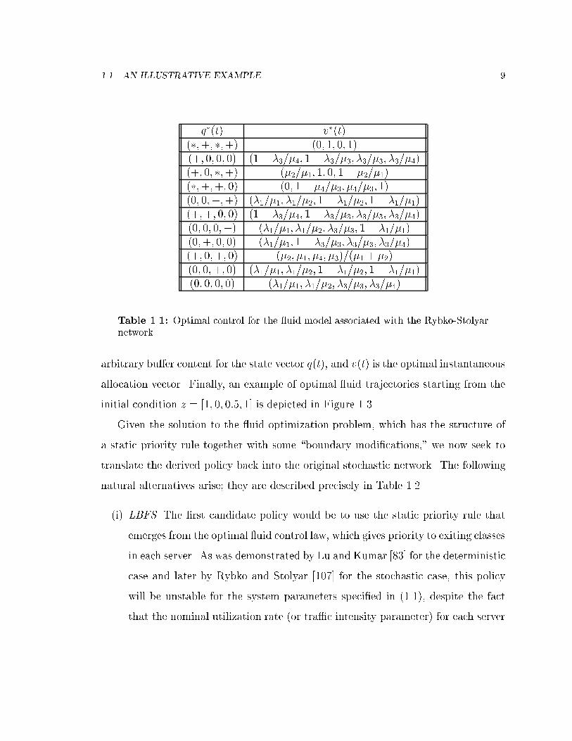
In more detail, the optimal control is the one described in Table 1.1, where a

\+" signi�es positive bu�er content, a \0" signi�es an empty bu�er, a \�" signi�es


q�(t) v�(t)(�;+; �;+) (0; 1; 0; 1)(+; 0; 0; 0) (1� �3=�4; 1� �3=�3; �3=�3; �3=�4)(+; 0; �;+) (�2=�1; 1; 0; 1� �2=�1)(�;+;+; 0) (0; 1� �4=�3; �4=�3; 1)(0; 0;+;+) (�1=�1; �1=�2; 1� �1=�2; 1� �1=�1)(+;+; 0; 0) (1� �3=�4; 1� �3=�3; �3=�3; �3=�4)(0; 0; 0;+) (�1=�1; �1=�2; �3=�3; 1� �1=�1)(0;+; 0; 0) (�1=�1; 1� �3=�3; �3=�3; �3=�4)(+; 0;+; 0) (�2; �1; �4; �3)=(�1 + �2)(0; 0;+; 0) (�1=�1; �1=�2; 1� �1=�2; 1� �1=�1)(0; 0; 0; 0) (�1=�1; �1=�2; �3=�3; �3=�4)

Table 1.1: Optimal control for the uid model associated with the Rybko-Stolyarnetwork

arbitrary bu�er content for the state vector q(t), and v(t) is the optimal instantaneous

allocation vector. Finally, an example of optimal uid trajectories starting from the

initial condition z = [1; 0; 0:5; 1] is depicted in Figure 1.3.

Given the solution to the uid optimization problem, which has the structure of

a static priority rule together with some \boundary modi�cations," we now seek to

translate the derived policy back into the original stochastic network. The following

natural alternatives arise; they are described precisely in Table 1.2.

(i) LBFS. The �rst candidate policy would be to use the static priority rule that

emerges from the optimal uid control law, which gives priority to exiting classes

in each server. As was demonstrated by Lu and Kumar [83] for the deterministic

case and later by Rybko and Stolyar [107] for the stochastic case, this policy

will be unstable for the system parameters speci�ed in (1.1), despite the fact

that the nominal utilization rate (or tra�c intensity parameter) for each server


0 1 2 3 4 5 6 70

1

0 1 2 3 4 5 6 70

1

0 1 2 3 4 5 6 70

1

2

0 1 2 3 4 5 6 70

1

q 1(t)

q 2(t)

q 3(t)

q 4(t)

Time

Figure 1.3: Optimal state trajectories in the uid model for z = [1; 0; 0:5; 1]

0 1 2 3 4 5 6 70

1

0 1 2 3 4 5 6 70

1

0 1 2 3 4 5 6 70

1

2

0 1 2 3 4 5 6 70

0.5

1

� Qn 1(t)

� Qn 2(t)

� Qn 3(t)

� Qn 4(t)

Time

Figure 1.4: State trajectories under LBFS/PR: Q(0) = 400[1; 0; 0:5; 1]; n = 400


is equal to 0:833, as follows:

�1 =�1�1

+�3�4

= 0:833 and �2 =�1�2

+�3�3

= 0:833: (1.7)

That is, the static priorities derived from the uid policy by neglecting \bound-

ary behavior" have catastrophic performance: they cause instability! Clearly,

the cost in (1.2) will still remain �nite, but when this policy is implemented over

long time horizons the queue length vector will eventually diverge to in�nity.

(ii) LBFS with priority reversal (LBFS/PR). Here each server uses LBFS as its

\default", but switches to the opposite priority when the other server's exit

bu�er is empty. It can be shown that this policy is stable, but its asymptotic

performance is not satisfactory, as explained below.

(iii) LBFS with server splitting (LBFS/SS). Here we implement exactly the optimal

policy derived form the uid model, splitting server e�ort in the prescribed

percentages from Table 1.1. Whenever one of the queue lengths is empty, any

positive server utilization predicted by the optimal uid control policy for this

class will not be implementable due to the discrete dynamics of the stochastic

network. In such cases, this percentage of server utilization will be reallocated

to the other class waiting to be processed at that server, if this is non-empty.

For example, when q = (0; 0;+;+) the optimal server allocation from the uid

control problem is (0:25; 1; 0; 0:75), yet the implemented server allocation in the

stochastic network will be (0; 0; 1; 1). This policy can also be shown to be stable,

but its asymptotic performance is not satisfactory, as explained below.

Using any one of the control policies just described, it is interesting to consider

system behavior under a sequence of initial conditions fzng, such that jznj ! 1as n ! 1, keeping all other system parameters �xed. Consider, for example, the

case where zn = n[1; 0; 0:5; 1]. Denoting by Qn(�) the four dimensional queue length


Q(t) LBFS LBFS/PR LBFS/SS(�;+; �;+) (0; 1; 0; 1) (0; 1; 0; 1) (0; 1; 0; 1)(+; 0;+;+) (0; 0; 1; 1) (1; 0; 1; 0) (�2=�1; 0; 1; 1� �2=�1)(+; 0; 0;+) (0; 0; 0; 1) (1; 0; 0; 0) (�2=�1; 0; 0; 1� �2=�1)(0; 0;+;+) (0; 0; 1; 1) (0; 0; 1; 1) (0; 0; 1; 1)(0; 0; 0;+) (0; 0; 0; 1) (0; 0; 0; 1) (0; 0; 0; 1)(+; 0;+; 0) (1; 0; 1; 0) (1; 0; 1; 0) (1; 0; 1; 0)(+; 0; 0; 0) (1; 0; 0; 0) (1; 0; 0; 0) (1; 0; 0; 0)(+;+;+; 0) (1; 1; 0; 0) (1; 0; 1; 0) (1; 1� �4=�3; �4=�3; 0)(0;+;+; 0) (0; 1; 0; 0) (0; 0; 1; 0) (0; 1� �4=�3; �4=�3; 0)(+;+; 0; 0) (1; 1; 0; 0) (1; 1; 0; 0) (1; 1; 0; 0)(0;+; 0; 0) (0; 1; 0; 0) (0; 1; 0; 0) (0; 1; 0; 0)(0; 0;+; 0) (0; 0; 1; 0) (0; 0; 1; 0) (0; 0; 1; 0)

Table 1.2: Implemented policies derived from uid optimal control in the Rybko-Stolyar network

process with initial state Qn(0) = zn, we de�ne the uid scaled version

�Qn(t) =Qn(nt)

n; 0 � t � T; (1.8)

and ask whether �Qn converges to a limit trajectory as n!1 that is optimal in the

uid model. (Because the scaling in (1.8) is that associated with the Law of Large

Numbers (LLN), one expects a deterministic limit to be approached.) Given the data

speci�ed in (1.1), the optimal uid trajectory is pictured in Figure 1.3.

For both LBFS/PR and LBFS/SS, the scaled processes �Qn do converge to a

deterministic limit as n!1, but that limit does not coincide with the optimal uid

trajectory pictured in Figure 1.3. That is, although these policies may be intended

as implementations of the optimal uid control policy, they do not in fact achieve as

their uid limits a trajectory that is optimal in the uid model. These two policies

fail to be asymptotically optimal because in both cases the servers are too slow in

switching from myopically draining cost out of the system to guarding against idleness

that will prevent optimal cost draining in future times. In fact, following this remark


n = 200 n = 400 n = 800LBFS 32.654 29.298 28.880

LBFS/SS 11.421 9.297 8.884LBFS/PR 11.175 8.224 7.709

Table 1.3: Fluid-scaled performance for Rybko-Stolyar network T = 7 andQn(0) =n[1; 0; 0:5; 1]

one would expect that the performance under LBFS/SS will be worse than that under

LBFS/PR.

The sub-optimal behavior explained above is depicted in Figure 1.4, where the

simulated output for the network operating under LBFS/PR starting from the initial

condition Q(0) = [400; 0; 200; 400] is shown. In the context of uid scaling described

above, these trajectories correspond to the case where Qn(0) = zn = n[1; 0; 0:5; 1]

with n = 400. Both axes in the plots of Figure 1.4 have been rescaled by n to re ect

that fact. For the nth system along this sequence of initial conditions, uid-scaled

cost over a horizon of length T can be calculated byZ T

0

�Qn(t)dt =1

n2

Z nT

0

Qn(t)dt;

this is a consequence of the uid scaling described above.

Table 1.3 summarizes some simulation results for the uid-scaled performance

under LBFS, LBFS/SS, and LBFS/PR. The initial conditions considered were of the

form Qn(0) = n[1; 0; 0:5; 1], and the horizon is set to T = 7, which is the time required

to drain the uid model under the optimal control computed earlier. These results

were obtained using exponentially distributed interarrival and service time random

variables. The minimum cost solution in the uid model that these performance

indexes should be compared to is 7:222. This is computed as the area under the

queue length plots in Figure 1.3.


From these results several observations are apparent. First, the �nite horizon per-

formance criterion under consideration is meaningful even for the case of the LBFS

policy, which would otherwise lead to instability in the Rybko-Stolyar network. Sec-

ond, all three policies described in Table 1.2 converge to a limiting cost that is not

optimal. This illustrates the subtlety of the translation step starting from the solu-

tion of a uid optimal control problem into an implementable policy in the original

stochastic network: successful translation involves relatively �ne structure.

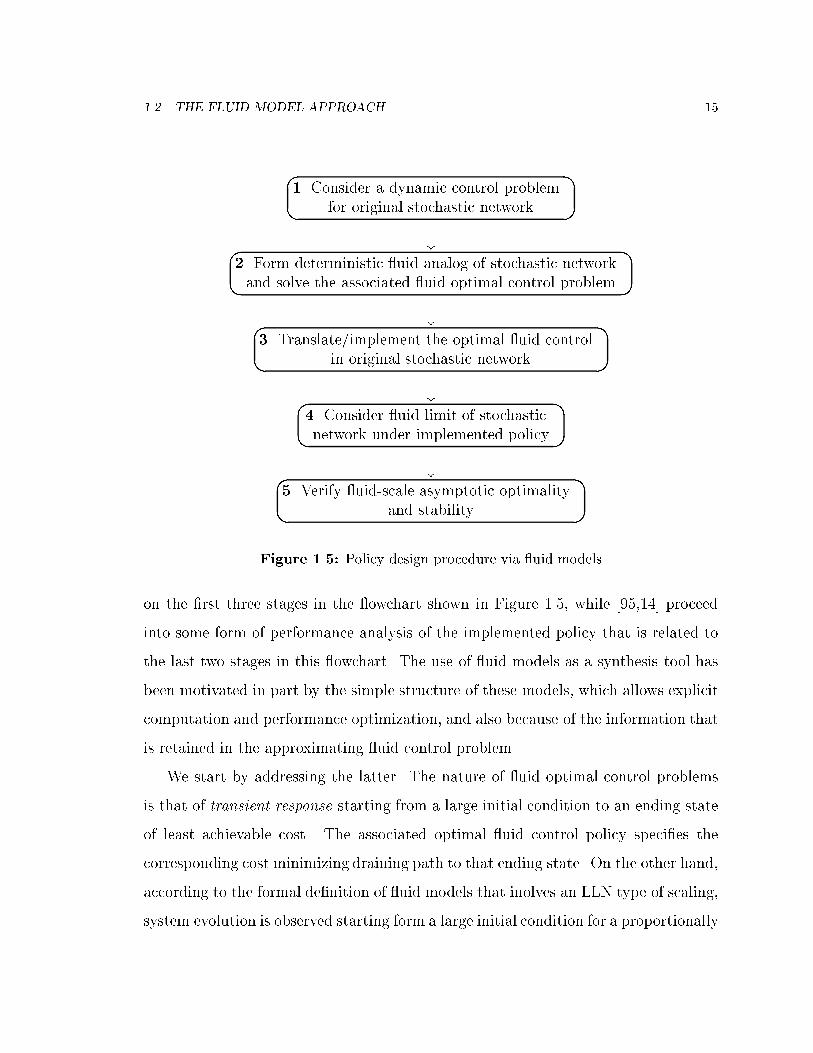
1.2 The uid model approach

The Rybko-Stolyar example helped to describe some necessary terminology, illustrate

the policy design procedure based on uid models, and also highlight some of the

obstacles that one needs to overcome in formalizing the approach. The following

owchart summarizes the necessary steps.

The focus on uid approximations originated through the recent developments

regarding these models and their imminent connection to the underlying stochastic

networks. The main motivation has been the important breakthrough in the theory

developed by Dai [31] that allowed stability analysis of multiclass queueing network

by examining their associated deterministic uid models; see also the works by Chen

and Mandelbaum [28], Rybko and Stolyar [107], Dai and Meyn [34], Dai and Weiss

[35], Chen [27], Stolyar [114], and Bramson [21,22,24]. Simultaneously, there has

been a growing literature in using uid models as a framework for synthesis and,

speci�cally, in using the solutions of uid optimal control problems in the design of

scheduling policies for the original stochastic networks. The �rst such reference is

the book by Newell [99], while more recent work can be found in Chen and Yao [29],

Atkins and Chen [5], Avram, Bertsimas and Ricard [6], Eng, Humphrey and Meyn

[43], Meyn [95], and Bertsimas and Sethuraman [14]. The results in [29,5,6,43] focus

1.2. THE FLUID MODEL APPROACH 15

�

�

�

1. Consider a dynamic control problem

for original stochastic network

j#�

�

�

2. Form deterministic uid analog of stochastic networkand solve the associated uid optimal control problem

j#�

�

�

3. Translate/implement the optimal uid control

in original stochastic network

j#�

�

�

4. Consider uid limit of stochasticnetwork under implemented policy

j#�

�

�

5. Verify uid-scale asymptotic optimality

and stability

Figure 1.5: Policy design procedure via uid models

on the �rst three stages in the owchart shown in Figure 1.5, while [95,14] proceed

into some form of performance analysis of the implemented policy that is related to

the last two stages in this owchart. The use of uid models as a synthesis tool has

been motivated in part by the simple structure of these models, which allows explicit

computation and performance optimization, and also because of the information that

is retained in the approximating uid control problem.

We start by addressing the latter. The nature of uid optimal control problems

is that of transient response starting from a large initial condition to an ending state

of least achievable cost. The associated optimal uid control policy speci�es the

corresponding cost minimizing draining path to that ending state. On the other hand,

according to the formal de�nition of uid models that inolves an LLN type of scaling,

system evolution is observed starting form a large initial condition for a proportionally


long time horizon, which essentially yields again a deterministic transient response

model. It is natural to expect that asymptotically the optimal transient behavior for

the uid scaled system will be close to the optimal achievable behavior in the uid

model. Indeed, such a result was established by Meyn in [94], therefore, suggesting the

analysis of the properties and structure of the latter in an e�ort to gain information

regarding the former. Apart from Meyn's positive �ndings, other simple results exist

that highlight the connection between the original optimal control problem and the

approximation embodied in the uid optimal control problem. For example, the c�

rule (see Chen and Yao [29] and Bertsimas, Paschalidis and Tsitsiklis [13]) and the

generalized c�-rule (see Newell [50] and VanMieghem [118]), are optimal for both the

underlying stochastic networks and their associated uid models. More generally, it

seems that whenever a static priority rule is optimal in the stochastic system then

the same priority rule will be optimal in the uid model as well.

Simultaneously, there are vast simpli�cations associated with these uid optimal

control problems. First, from an analysis point of view, one has access to the extensive

literature on optimal control for deterministic systems with continuous dynamics that

has been developed within the �eld of control theory; see, for example, the books by

Athans and Falb [4], Bryson and Ho [25], and Bertsekas [11]. And second, from a

computational viewpoint, the simple structure of uid models has been exploited by

many researchers in proposing e�cient algorithms that perform well both in theory

and in practice [102{104,122,124,85,88]. Most of these algorithms primarily focus on

linear cost structures, but non-linear and convex cost functions can also be addressed

e�ciently. All these observations motivate uid model analysis as a means for the

design of near-optimal scheduling policies for the underlying stochastic processing

networks and lend credibility to the described policy design procedure.

In stage 3, the optimal uid control policy is translated into an implementable

policy in the stochastic network. Stages 4 and 5 describe a criterion for performance

1.2. THE FLUID MODEL APPROACH 17

analysis under the implemented policy that is consistent with the model approxi-

mation adopted at stage 2, in the following sense: the implementation is tested for

asymptotic optimality in the limiting parameter regime where the model approxima-

tion is valid. This property is referred to as uid-scale asymptotic optimality (FSAO),

and it was �rst described by Meyn in [95], in the context of performance analysis under

uid scaling, in his work on designing scheduling policies via value or policy iteration

procedures using uid model approximations. The proposed criterion of FSAO has

the same degree of �delity as the uid analog, or uid model approximation used

in stage 2. It tests whether optimality is achieved in the limiting regime where the

network control problem reduces to one of uid (or transient) optimization, the so-

lution of which was used in designing this policy in stage 3. This is a \minimal"

requirement for the implemented policy, which in comparison to the original problem

at hand, it provides a relaxed notion of optimality that appears to be much simpler

and one that hopefully could be achieved even for general multiclass networks. On

the same token, in the spirit of the positive results mentioned earlier regarding the

connections between optimal behavior in the stochastic network to that in the uid

model, the premise of the uid model approach to network control problems is that

despite this \weak" criterion of what constitutes a \good" control policy, this relaxed

notion of optimality will guide us in designing \near-optimal" policies for the original

stochastic network control problems. Finally, apart from FSAO, we also require that

the original stochastic network is stable under the implemented policy.

Despite the apparently modest objective of FSAO, the meaning of the uid policy

in the original network is subtle. As it was demonstrated through the analysis of

the Rybko-Stolyar example, although the associated uid optimization problem is

\trivial," each of three \obvious" interpretations in the stochastic network is \wrong."

In fact, given the solution of the associated uid optimal control problem, which is

presumably easily computable, it is surprisingly di�cult to translate the optimal uid


control policy into an implementable policy in the original stochastic network, due to

the �ner structure of the original network model. A few simple networks have been

analyzed in the papers cited above [29,6,43,95], but no general mechanism has been

constructed that guarantees uid-scale asymptotic optimality or even stability for the

policy extracted from the uid solution.

The same problem of back-translation has been observed in the context of the

heavy-tra�c approach to network control problems pioneered by Harrison and others

[52,60,61,125,78,91,54]. There, one would follow exactly the same owchart of Figure

1.5, while replacing uid by Brownian models. These are di�usion approximating

models of the stochastic networks under investigation. In the latter, limiting behav-

ior of appropriately scaled processes (according to a central limit theorem type of

scaling) is examined as the load on a system approaches its capacity limit, which

is referred to as the \heavy-tra�c regime." The notion of asymptotic optimality is

appropriately modi�ed in order to examine system behavior as one approaches the

limiting \heavy-tra�c" regime approximated by the Brownian model dynamics. As

with the uid model approach, the translation of the solution of a Brownian con-

trol problem is hard, and satisfactory results have only be achieved in isolated and

simple examples [60,61]. The �rst general translation mechanism was proposed by

Harrison [54] in his BIGSTEP approach to dynamic control for stochastic networks.

BIGSTEP was described in the context of Brownian models and heavy-tra�c limits

and it was rigorously proved to be asymptotically optimal (in the heavy-tra�c sense)

for a simple two station example [56].

In summary, the main obstacle that needs to be addressed in order to formal-

ize the uid model approach described in Figure 1.5, is in �nding a mechanism to

translate the solution of an associated uid optimal control problem into an imple-

mentable control policy in the stochastic network in a way that guarantees certain

desirable properties. This will be the central topic of this thesis, and speci�cally,

1.3. THESIS OUTLINE 19

our main contribution is in proposing and analyzing such a translation mechanism

that addresses and solves this problem. In passing, we will formally introduce the

FSAO criterion, establish the stability of the proposed class of policies, and �nally,

consider many other extensions that generalize the performance criteria of interest as

well as the class of stochastic networks that can be analyzed in the proposed frame-

work. These extensions will also provide solutions that are computationally more

e�cient and thus, more scalable with respect to the size of the networks that can be

considered.

The family of policies we describe is based on the idea of a discrete-review struc-

ture of the BIGSTEP approach [54]. Each discrete-review policy in the family to be

investigated will be derived from the solution of a uid optimal control problem of

interest. In such a policy, system status is reviewed at discrete points in time, and at

each such point the controller formulates a processing plan for the next review period

based on the queue length vector observed. Formulation of the plan requires solution

of a linear program whose objective function involves data from the solution of the

uid optimization problem that one starts with. Implementation of the processing

plan involves enforcement of certain safety stock requirements in order to avoid un-

planned server idleness. Review periods and magnitudes of safety stocks increase as

queues lengthen, but both grow less-than-linearly as functions of queue length and

hence are negligible under uid scaling. During each review period the system is

only allowed to process jobs that were present in the beginning of that period, which

makes the implementation of processing decisions very simple.

1.3 Thesis outline

The organization of this thesis is as follows. Chapter 2, is an overview of the basic

ideas regarding multiclass networks and their associated uid models. It also contains


a discussion of uid optimal control problems and a formal de�nition of the key

property of uid-scale asymptotic optimality; these results are from [86]. In order

to simplify the exposition, the main part of this thesis will concentrate to network

models where only scheduling decisions are to be made. This will be extended in

chapter 5.

Chapter 3, describes and analyzes a family of discrete-review policies that is stable

and asymptotically optimal under uid scaling. This family of policies is based on

Harrison's BIGSTEP approach [54], which is here extended and precisely de�ned and

analyzed in the general setting of open multiclass networks. The results presented in

this chapter are from [87,86].

In chapter 4, putting aside all considerations of system optimality, and given any

feasible uid trajectory, a discrete-review policy is described which achieves as its uid

limit this trajectory. This class of trajectory tracking policies is intuitively appealing

and also quite general, and includes, for example, uid scale asymptotically optimal

policies as a special case. The results of this chapter can be found in [86,89].

In chapter 5 several extensions of the methodology of chapters 2 - 4 are presented.

First, a new family of uid control policies is described and the properties of the

corresponding discrete-review policies are stated. Second, several extensions of the

network models under investigation are presented and the family of proposed policies

is appropriately augmented for this more general class of networks. Several contrived

assumptions imposed in the mathematical models of multiclass networks, such as the

absence of setup times or batch processing or multi-server stations, will be removed.

This will illustrate the power of the proposed approach and demonstrate its practical

appeal. Some of these results of this chapter are form [87,90].

Finally, chapter 6 contains a summary of this work, some concluding remarks, and

some remarks on future directions of research both on the theoretical and practical

frontiers.

Chapter 2

Network models

This chapter describes open multiclass queueing networks and their associated uid

models. The de�nitions of stability for both network models are presented, the canon-

ical network optimal control problem and its associated uid optimal control problem

are analyzed, and �nally the notion of uid-scale asymptotic optimality is introduced.

The following notation will be useful. Let R+ = [0;1). CR[0;1) denotes the

space of continuous functions on R+. DR[0;1) is the space of right continuous

functions on R+ having left limits on (0;1) (RCLL), endowed with the Skorohod

topology; see Ethier and Kurtz [44, section 3.5]. Given a sequence of functions ffng,where fn 2 DR[0;1) for each n and a function f 2 CR[0;1), fn ! f in the Skorohod

topology if and only if fn ! f uniformly on compact sets (u.o.c.). That is,

sup0�s�t

jfn(s)� f(s)j ! 0; as n!1:

The vector of ones of appropriate dimension will be denoted by 1, bxc will be the

integer part of x rounded down, x^y = min(x; y), x_y = max(x; y), x+ = max(0; x),

and �nally all vector equalities or inequalities should be interpreted componentwise.

The transpose of a matrix P will be denoted P 0, diagfx1; : : : ; xng will denote the

n� n diagonal matrix with diagonal elements (x1; : : : ; xn).

21

22 CHAPTER 2. NETWORK MODELS

2.1 Multiclass open queueing network models

In the description of a multiclass queueing network we adopt the setup introduced

by Harrison [52]. Consider a queueing network of single server stations indexed by

i = 1; : : : ; S. (The terms station and server will be used interchangeably.) The

network is populated by job classes indexed by k = 1; : : : ; K and in�nite capacity

bu�ers are associated with each class of jobs. Class k jobs are served by a unique

station s(k) and their service times are f�k(n); n � 1g. That is, the nth class k job

requires �k(n) time units of service from station s(k). Jobs within a class are served

on First-In-First-Out (FIFO) basis. Upon completion of service at station s(k), a

class k job becomes a job of class m with probability Pkm and exits the network with

probability 1�Pm Pkm, independent of all previous history. Assume that the general

routing matrix P = [Pkm] is transient (that is, I + P + P 2 + : : : is convergent). Let

f�k(n)g denote the sequence of K-dimensional IID Bernoulli random vectors such

that �kj (n) = 1 if upon service completion the nth class k job becomes a class j job

and is zero otherwise, and let �k(n) =Pn

j=1 �k(j). Every job class k can have its own

exogenous arrival process with interarrival times f�k(n); n � 1g. The set of classes

that have a non-null exogenous arrival process will be denoted by E and the the

notation E(t) will be used to signify the K-dimensional vector of exogenous arrivals

in the time interval [0; t]. It is assumed that E 6= ;.We make the following assumptions on the distributional characteristics of the

arrival and service time processes:

(A1) �1; : : : ; �K and �1; : : : ; �K are mutually independent, positive, IID sequences;

(A2) E[�k(1)] 6= 0 for k = 1; : : : ; K: For some � > 0; E[e��k(1)] < 1 for k =

1; : : : ; K and E[e��k(1)] <1 for k 2 E ;

(A3) For any x > 0; k 2 E ; Pf�k(1) � xg > 0. Also, for some positive function

2.1. MULTICLASS OPEN QUEUEING NETWORK MODELS 23

p(x) on R+ withR10p(x)dx > 0, and some integer j0, P

nPj0i=1 �k(i) 2 dx

o�

p(x)dx.

Condition (A1) can be relaxed; see the remark after Proposition 2.1 of Dai [31]. (A2)

is stronger than the �nite �rst moment condition usually imposed (see, for example,

Dai [31]), and it is needed in the derivation of large deviation bounds required in our

analysis. This condition is satis�ed for f�k(n)g. The technical regularity conditions

in (A3) are imposed so that we can make use of the general stability theory of Dai

[31,34]; these conditions are never invoked in propositions which are actually proved

in this work.

For future reference, let �k = 1=E[�k(1)] and �k = 1=E[�k(1)] = 1=mk be the

arrival and service rates respectively for class k jobs, let � = (�1; : : : ; �K)0, and let

M = diagfm1; : : : ; mKg. The set fk : s(k) = ig will be denoted Ci and is called

the constituency of the server i, while the S �K constituency matrix C will be the

following incidence matrix:

Cik =

8<: 1 if s(k) = i

0 otherwise.

Given the Markovian routing structure of these networks one can compute the

vector of e�ective arrival rates, denoted �, by the following set of linear equations,

commonly called the tra�c equations,

�k = �k +KXi=1

�iPik; k = 1; : : : ; K: (2.1)

Since P is transient the vector of e�ective arrival rates can be computed by

� = (I � P 0)�1�:

Hereafter, it will be assumed that � > 0. That is, the e�ective arrival rate at each class

is strictly greater than zero. This restriction is not critical, and is mainly imposed in


order to simplify the policy description of section 3.1. Appropriate modi�cations will

be provided in order to extend the relevant results to the case where no restrictions

are imposed on the �k's.

The average load contributed by class k jobs to server s(k) will be �k=�k and the

average utilization level or tra�c-intensity of each server will be

�i =Xk2Ci

�k�k; i = 1; : : : ; S: (2.2)

Letting R = (I � P 0)M�1, (2.2) can be written in vector form as

� = CR�1�: (2.3)

Denote by Qk(t) the total number of class k jobs in the system at time t, and

by Q(t) the corresponding K-vector of \queue lengths". A generic value of Q(t) will

be denoted by q, and the size of this vector is de�ned as jqj = Pk qk. (To avoid

confusion the reader should note that jAj will also denote the cardinality of a set A,

but the intended use of the notation will always be clear.) Let y denote the initial

condition of the network, which apart from the initial queue length con�guration it

might include other information regarding the initial state of the system; this will

become clearer in chapter 3 where a speci�c example will be described.

A scheduling policy is a rule according to which resource allocation decisions

are made over time starting from an initial condition y. It takes the form of a K-

dimensional cumulative allocation process fT y(t); t � 0; T y(0) = 0g, where T yk (t)

denotes the time allocated by server s(k) into serving class k jobs up to time t, and the

superscript \y" denotes the dependence on the initial condition. Since the process T y

is Lipschitz, one can de�ne its derivative _T y(t) , dT y(t)=dt, where _T yk(t) will be the

fraction of e�ort allocated into processing class k jobs by server s(k) at time t. For an

admissible policy, _T y(t) is non-negative, it satis�es the capacity constraints C _T y(t) �1, and also _T y

k (t) can only be positive if Qk(t) > 0. In addition, an admissible

2.1. MULTICLASS OPEN QUEUEING NETWORK MODELS 25

policy needs to be non-anticipating (or causal), which, roughly speaking, ensures that

_T y(t) only depends on information available up to time t and does not require future

information. In mathematical terms this translates to a measurability condition with

respect to the appropriate �ltration generated up to time t that also depends on

the scheduling policy applied. For purposes of this thesis we will avoid a precise

statement of this condition, since it will not be required towards the development

of our results and it would otherwise involve a fairly subtle and technical exposition.

Unless otherwise speci�ed, it should be assumed that each server can only process one

job at a time, and that _T yk (t) is either equal to 1 if a class k job is being processed or

0 otherwise. For concreteness we assume non-preemptive type of service. Let Iy(t) be

the I-dimensional cumulative idleness process de�ned by Iy(t) = 1t� CT y(t), where

Iyi (t) is the total time that server i has been idled up to time t. The process Iy(t)

has to be non-decreasing, which re ects the resource capacity constraints. A generic

admissible policy that satis�es all of the above conditions will be denoted by �.

Given any admissible scheduling policy, a Markovian state descriptor can be con-

structed and an underlying Markov chain can be identi�ed for the controlled network.

The Markovian state is based on the queue length vector, as well as other auxiliary

quantities that depend on the distributional characteristics of the interarrival and

service processes and on the scheduling rule used. The Markovian state at time t will

be denoted by Y (t) and the corresponding normed state space will be (Y; k � k); seethe comments by Dai and Meyn [34, section IIb] or Bramson [24, section 3] regarding

the choice of k � k. Examples of such Markov chain constructions can be found in

Dai [31]. Hereafter, whenever a new class of policies is introduced the appropriate

Markov chain descriptor will be identi�ed.

Let y 2 Y be the initial state of the network under a given admissible policy.

Denote by Ra(t) the jEj-vector of remaining times until the next external arrivals at

the various classes, and by Rs(t) the K-vector, where its kth component is equal to


the remaining service time for the class k job currently being processed. De�ne the

following quantities:

Eyk(t) = maxfn : Ra(0)k + �k(1) + � � �+ �k(n� 1) � tg; t � 0; k 2 E ;Syk(t) = maxfn : Rs(0)k + �k(1) + � � �+ �k(n� 1) � tg; t � 0:

Eyk(t) is the number of exogenous arrivals of class k up to time t and Sy

k(t) is the

number of service completions of class k jobs if server s(k) devoted t time units in

processing class k jobs. Also, �kl (n) denotes the total number among the �rst n class

k jobs that upon service completion became class l jobs, which is independent of the

initial condition y.

The following equations (here expressed in vector from) were �rst derived by

Harrison in [52] to obtain Brownian models with control capability and they were

later re�ned by Harrison and Nguyen [58] for the case of FIFO scheduling. Recall

that T yk (t) is the amount of time that server s(k) devoted into processing class k jobs

up to time t and let z denote the initial queue length con�guration, which is speci�ed

by the initial condition y. The queue length dynamics are described by

Q(t) = z + Ey(t) +KXk=1

�k(Syk(T

yk (t)))� Sy(T y(t)): (2.4)

Finally, the canonical class of network control problems addressed in this work is

described. Let g : RK+ ! R+ be a C2 convex cost rate function such that, for some

constants b; c;�b; �c > 0 such that b � �b, c � �c, and

bjxjc � g(x) � �bjxj�c: (2.5)

Note that (2.5) implies that g(x) = 0 , x = 0. Given the cost rate function g,

the following stochastic network control problem is considered: choose an allocation

process T (t), or equivalently, an admissible policy �, in order to minimize

J�T (z) = E�z

Z T

0

g(Q(t))dt; (2.6)

2.2. FLUID MODELS 27

where E�z denotes the expectation operator with respect to the probability measure

P�z de�ned by any admissible policy � and initial condition z. The use of T with

no time argument will denote a time horizon and should not be confused with the

cumulative allocation T (t).

In this problem formulation attention is restricted to �nite horizon network control

problems. It is convenient to think of T as being long but �nite. The objective in

these problems remains �nite starting from an arbitrary (but �nite) initial condition

independent of the tra�c intensity (or load) at each station, and in particular, this

problem remains meaningful even when � � 1 where, for example, long run averages

will not exist. This will allow for an easy extension to the heavy-tra�c regime, where

�! 1. This case will be addressed brie y in chapter 4.

2.2 Fluid models

Consider a sequence of initial conditions fyng � Y such that kynk ! 1 as n ! 1and for any real valued process ff(t); t � 0g de�ne its uid scaled counterpart by

�fn(t) =1

kynkfyn(kynkt): (2.7)

In the sequel, the overbar notation will signify uid scaled quantities and appropriate

superscripts will be used to signify the scaled processes corresponding to some initial

condition along the sequence fyng. In order to avoid the use of double superscripts

the dependence to the initial condition yn will be denoted by a single superscript n.

A functional strong law of large numbers (FSLLN) can be derived for the uid-

scaled processes de�ned above. The following is Lemma 4.2 in Dai [31].

Lemma 2.2.1 Let fyng � Y such that kynk ! 1 as n!1. Assuming that

limn!1

�Rna(0) =

1

kynkRna(0) = �Ra and lim

n!1

�Rns (0) =

1

kynkRns (0) = �Rs;


as n!1, almost surely

1

kynk�k(bkynktc)! P 0

kt; u.o.c. (2.8)

1

kynkEnk (bkynktc)! �k(t� �Ra)

+; u.o.c. (2.9)

1

kynkSnk (bkynktc)! �k(t� �Rs)

+; u.o.c.: (2.10)

The limit processes in (2.8)-(2.10) are deterministic and continuous. Continuity fol-

lows from the fact that the jump size of the scaled processes is decreasing as 1=kynk,which yields continuous limit trajectories. The deterministic nature of these limits is

a direct consequence of the FSLLN scaling. Note that the limits �Ra; �Rs depend on

the sequence fyng.Applying the scaling of (2.7) to (2.4) and using (2.8)-(2.10) the following result is

obtained.

Theorem 2.2.1 [31, Theorem 4.1] For almost all sample paths ! and any sequence

of initial conditions fyng � Y such that kynk ! 1 as n!1, there is subsequence

fynj(!)g with kynj(!)k ! 1 such that

( �Qynj (0; !); �Rynja (0; !); �Rynj

s (0; !)! (q(0; !); �Ra(!); �Rs(!)) (2.11)

( �Qynj (t; !); �T ynj (t; !))! (q(t; !); �T (t; !)) u.o.c.: (2.12)

Furthermore, (q(�; !); �T (�; !)) satis�es the following set of equations

q(t) = q(0) + �(t1� �Ra)+ � (I � P 0)M�1( �T (t)� �Rs)

+; (2.13)

q(t) � 0 for t � 0; (2.14)

�I(t) = 1t� C �T (t); �T (0) = 0; (2.15)

�T (t); �I(t) are non-decreasing for t � 0; (2.16)

together with some additional conditions on (q(�; !); �T (�; !)) that are speci�c to the

scheduling policy employed.

2.2. FLUID MODELS 29

That is, the uid limits depend on ! and on the converging subsequence fynjg as

well (through �Rs; �Ra). They are neither deterministic nor unique, but their dynamics

are captured by these deterministic and continuous equations of evolution (2.13)-

(2.16). Hereafter. whenever possible the dependence on ! will be suppressed from

the notation.

The above set of equations will be referred to as the delayed uid model associated

with a multiclass queueing network under a speci�ed scheduling policy. Moreover,

we will say that (q; �T ) 2 FM -or equivalently that it is a uid solution- if this pair

of state and input trajectories satis�es equations (2.13)-(2.16). It is immediate from

(2.13)-(2.16) that the limit processes (q; �T ) are Lipschitz continuous. Hence, it follows

that that they have a time derivative almost everywhere; see Lemma 2.1 of Dai and

Weiss [35]. A path q(�) is called regular at t if it is di�erentiable at t and its derivativeat time t will be denoted by _q(t). Let v(t) denote the instantaneous uid allocation

vector at time t. The cumulative allocation process can be rewritten as

�T (t) =

Z t

0

v(s)ds; t � 0:

Restricting attention to the case where �Ra = �Rs = 0 and using the a.e. di�eren-

tiability of the limit processes, for almost all times t � 0 the uid limit model can

be expressed as a linear dynamical system with polytopic constraints in v(t) of the

following form:

_q(t) = �� Rv(t); q(0) = z; (2.17)

q(t) � 0; Cv(t) � 1; v(t) � 0 for t � 0; (2.18)

together with some policy speci�c conditions. The uid limit model in (2.17)-(2.18)

is called undelayed. This is the only case studied in the sequel. Once again, the

dependence of the uid limits on the sample path ! has been suppressed. (In the

literature the term undelayed refers to the set of integral equations (2.13)-(2.16) for


the case where �Ra = �Rs = 0.) Following our earlier notation we will say that that

(q; v) 2 FM -or equivalently that it is a uid solution- if this pair of state and input

trajectories satisfy equations (2.17)-(2.18). Undelayed limits can be obtained if one

restricts attention to exponential interarrival and service time processes, or in the

case of general distributions, if one lets kynk ! 1 while keeping Rna(0) and R

ns (0)

bounded.

For further descriptions of the derivation of the desired uid limit model and a

discussion on delayed and undelayed limits the readers could refer to Dai [31,32] and

Bramson [24, section 4].

2.3 Stability

The following de�nitions of stability are from Dai [31]. An excellent reference on this

material is the recent book by Meyn and Tweedie [96]. Let BY be the Borel �-�eld

of Y. Let �A = infft � 0 : Y (t) 2 Ag. The process Y (t) is Harris recurrent if thereexists some �-�nite measure � on (Y;BY ) such that whenever �(A) > 0 and A 2 BY ,

Py(�A <1) = 1:

If Y is Harris recurrent then an essentially unique invariant measure � exists. If the

invariant measure is �nite, then it may be normalized to a probability measure; in

this case Y is positive Harris recurrent.

De�nition 2.3.1 A multiclass network under a speci�c scheduling policy is stable if

the underlying Markov chain is positive Harris recurrent.

Intuitively, positive Harris recurrence of the underlying Markov chain implies that

the queue length process will remain �nite for all t � 0. A necessary condition for

stability is that the tra�c intensity at each station is less than one. That is,

� = CR�1� < 1: (2.19)

2.3. STABILITY 31

Through a series of celebrated counterexamples it has been shown that this condition

is not su�cient in establishing stability under a given policy. Speci�cally, the exam-

ples developed by Lu and Kumar [83], Rybko and Stolyar [107] (this is the example

studied in chapter 1), Bramson [18{20], Seidman [108], Dumas [41] and others show

that networks can exhibit instability phenomena even though the tra�c intensity

parameter is less than one at each station. Roughly speaking, in all these examples

instability occurs under by exciting periodic blockage and starvation patterns that

force excessive idleness to be incurred at the various servers in the network. These

counterexamples have stimulated a lot of work on the stability of multiclass networks

and speci�cally, they have motivated the study of uid models for stability analysis

of queueing networks.

Fluid models were �rst introduced as part of a stability analysis of a multiclass

network in the work by Rybko and Stolyar [107] for the speci�c network described in

chapter 1. Subsequently, the following key observation due to Dai [31] initiated most

of the work in the uid model approach to stability analysis of multiclass networks.

Dai showed in Theorem 3.1 in [31] that if there exists a � > 0 such that

limkyk!1

1

kyk E[kYy(kyk�)k] = 0; (2.20)

then we can construct a Lyapunov function to establish that the underlying Markov

chain is positive Harris recurrent. Thus, (2.20) allows us to establish stability by

studying \ uid" scaled processes obtained according to (2.7). In light of (2.20),

stability in the uid model is de�ned as follows:

De�nition 2.3.2 The uid model associated with a scheduling policy is stable if there

exists a time T > 0 such that for any solution q(�) of the uid model equations with

jq(0)j = 1, q(t) = 0, for t � T .

Using (2.20), Dai proved the following important result that relates the stability

properties of the uid model to that of the underlying queueing network.


Theorem 2.3.1 [31, Theorem 4.2] A multiclass open queueing network is stable

under a scheduling policy if the associated delayed uid model is stable.

Thus, the veri�cation of stability of a multiclass network under a speci�ed policy is

reduced to the much simpler task of checking stability of a uid model with piecewise

linear dynamics. For the case of non-idling or work-conserving uid limits, these are

uid solutions (q; v) that satisfy the condition

(1� Cv(t))0Cq(t) = 0; for all t � 0; (2.21)

Chen further re�ned this Theorem in [27, Theorem 5.2] by establishing the following

condition: the uid model equations (2.13)-(2.16) and (2.21) are stable if and only if

(2.17)-(2.18) and (2.21) are also stable. Although this condition reduces the task of

checking stability to an analysis of the simpler undelayed uid model equations, in

general one needs to establsh stability under a whole family of policies that satisfy the

non-idling constraint in (2.21), which is very conservative. The following modi�cation

of Chen's condition is su�cient in order to establish stability by analyzing a single

policy of interest.

Proposition 2.3.1 Consider any scheduling policy such that its associated uid limit

model satis�es condition (2.21). Suppose that for any B > 0 there exists a time TB

such that for any solution q(�) of the undelayed uid equations with jq(0)j � B,

q(t) = 0, for all t � TB. Then, the delayed uid model is also stable.

Proof. Consider any uid solution of the (delayed) uid model equations. By the

non-idling property, it follows that there exists a time t0 such that �T (t0) � �Rs and

t01 � �Ra. At time t0 we have that

q(t0) = ~z + �t0 �R �T (t0);

where ~z = z � diagf�g �Ra + R �Rs. Let B = jq(t0)j. By assumption it follows that

q(t) = 0 for any t � t0 + TB, which completes the proof. 2

2.3. STABILITY 33

The apparently stronger condition of establishing stability starting for any com-

pact set of initial conditions is required in order to avoid potential pathological cases

of dynamic control policies whose behavior changes drastically when the state is large.

For example, consider the Rybko-Stolyar network of chapter 1 operating under LBFS

if jq(t)j > 1 and any other strict priority rule if jq(t)j � 1. In this case, the undelayed

uid model will be stable if jq(0)j � 1 and unstable otherwise. The condition of

Proposition 2.3.1 is automatically satis�ed in cases where a certain similarity prop-

erty of the uid limits applies (see Stolyar [114, section 6] or Chen [27, section 2]),

and it is also true in all cases where this proposition will be invoked in the sequel.

Let S denote that set of uid solutions (q; v) that satisfy (2.17)-(2.18) and let Lbe the set of uid limits obtained using the formal limiting procedure in Theorem

2.2.1. It is instructive to note that in general the following is true

L � S: (2.22)

That is, the equations obtained by the uid limit procedure may admit feasible uid

solutions that cannot be obtained as formal limits of uid scaled processes of the

underlying stochastic network. Hence, proving stability by analyzing all uid solutions

in S is su�cient but not necessary in general. Only partial results have been derived

in the converse direction by Meyn [93], Dai [33] and Stolyar [114]; these are instability

criteria based on uid model analysis. A general discussion of the results presented

in this section can be found in the review article by Dai [32] and some additional

insightful comments are given in Bramson [24, section 4].

Overall, the uid model approach to stability analysis of multiclass networks has

been used extensively over the past few years. Most often the research e�orts has

been focused in the complete characterization of the stability region of these networks;

this is the region in which the network will be stable under any non-idling scheduling

policy. For example, see the work by Dai [31], Bertsimas, Gamarnik and Tsitsiklis


[12], and Kumar and Meyn [69]. In a few other cases, speci�c policies -or classes of

policies- have been proved to be stable, mainly for the class of networks referred to

as re-entrant lines; examples can be found in the work of Kumar [68], Kumar and

Kumar [71], Dai [31] and Bramson [21,22,24].

2.4 Fluid optimal control problems

According to the uid model approach to network control problems, the �rst step is to

replace the optimal control problem for the stochastic network by an associated uid

optimal control problem. The methodology was illustrated in chapter 1 in relation

to a simple two-station network. Here, the general case is presented. The uid

optimization problem associated with (2.6) is de�ned by

�V g(z) = minv(�)

�Z T

0

g(q(t))dt : q(0) = z and (q; v) 2 FM�: (2.23)

�V g(z) denotes the value function of the uid optimization problem starting from the

initial condition z, the superscript g denotes the dependence on the cost rate function,

and T is the same time horizon that appears in the performance index in (2.6). The

problem in (2.23) is one of transient optimization or transient recovery starting from

a large initial backlog. One should think of T as being long enough so that starting

from any appropriately normalized initial condition z, the transient behavior of the

optimal solution will have settled and the queue length vector will have reached its

�nal state of least achievable cost without being a�ected by the �nite horizon T .

Speci�cally, optimization in the uid model gives information about the path that

the state will follow until it reaches a \�nal" state; for � < 1 this state is at the origin,

for � = 1 this is the state of minimum achievable cost given the initial condition, and

if � > 1 this state will correspond to the asymptote of minimum cost accumulation,

along which the uid trajectory will blow up as t increases.

2.4. FLUID OPTIMAL CONTROL PROBLEMS 35

2.4.1 Characterization of optimal control policies

First, note that the control v(t) = R�1� for 0 � t � T is feasible and moreover, it

provides the following upper bound on the value function: 0 � �V g(z) � Tg(z): More-

over, given the properties of the cost rate function g, it follows that the objective in

(2.23) is continuous in z and thus, the resulting optimization problem is of the form

of minimization of a continuous function in a compact set. Existence of an optimal

solution follows from Weiertrass Theorem; the reader is referred to Luenberger [84]

for a detailed exposition. Given a compact set of initial conditions fz : jzj � Bg, andusing the Lipschitz continuity of the uid trajectories q(�), we can bound above the

set of feasible uid solutions of (2.23) by BT�, where � is an appropriate growth con-

stant determined by � and R. Then G = supfrg(q)0(��Rv) : v 2 V(q); jqj � BT�g,where V(q) = fv : v � 0; Cv � 1; (Rv)k � �k for all k such that qk = 0g is the setof admissible controls when the state is q. Note that the set of admissible controls

is non-empty, since R�1� 2 V(q) for all q � 0. Using this de�nition, G is a Lips-

chitz constant for g and consequently for the objective of (2.23) as well. This implies

almost everywhere di�erentiability of the value function �V g over the set of initial con-

ditions z � B. A generalized derivative can be de�ned (by choosing an appropriate

subgradient) at points where �V g is not di�erentiable. Since g is C2 it follows that

the generalized gradient of �V g, denoted r �V g, will also be a.e. continuous. Hereafter,

we make the stronger assumption that r �V g is in fact everywhere continuous; this as-

sumption is not restrictive, since one could always construct a smooth approximation

of any optimal uid trajectory that is arbitrarily close to it, and proceed by analyzing

this smooth approximation (that has a continuous gradient) thereafter.

The optimal instantaneous allocation is a state feedback law that can be charac-

terized by a direct application of dynamic programming principles; see for example

Bertsekas [10, section 3.2] for background information and a derivation based on the

Hamilton-Jacobi-Bellman equation and the maximum principle. The following is an


informal derivation of the optimality conditions for the solution of this problem in

terms of the cost-to-go function of the optimal control problem, denoted �V g(q(t); t).

Note that the cost-to-go is a function of the current state and the time t; this is

a consequence of the �nite control horizon T . In this notation, �V g(z) should read

�V g(z; 0).

�V g(q(t); t) = g(q(t))�t+ minv2V(q(t))

�V g(q(t+ �t); t+ �t) + o(�t) (2.24)

= g(q(t))�t+ �V g(q(t); t) +d

dt�V g(q(t); t)�t+

+ minv2V(q(t))

r �V g(q(t); t)0(�� Rv)�t+ o(�t): (2.25)

The optimal control v(t) is computed as the solution of the following linear program

v(t) = argminv2V(q(t))

r �V g(q(t); t)0(�� Rv) = argmaxv2V(q(t))

r �V g(q(t); t)0Rv: (2.26)

As a �rst application of the stability theory described in the previous section we

prove the following proposition:

Proposition 2.4.1 Assuming that �i < 1 at every station i, there exists a constant

Tg that depends on the cost rate function g(�), such that for any T > T g the uid

model (2.17), (2.18) and (2.26) is stable.

Proof. Given an initial condition z, an input control v(t) will be constructed that

will linearly translate the state, starting from z back to the origin. (In the sequel, all

quantities related to this construction will be denoted by a \hat".) Let T (t) be the

total allocation process associated to the instantaneous input control v(t) and let t�

be the time that the uid network will empty under this control. Rewrite equation

(2.17) in the form

q(t) = z +RY (t); where Y (t) = R�1�t� T (t):

In this case, Y (t�) = �R�1z and thus T (t�) = R�1�t� + R�1z. Linear translation

from z back to the origin implies that v(t) = T (t�)=t� for all t � t�. By the de�nition


of R it follows that R�1 =M(I �P 0)�1 =M(I +P +P 2+ � � �), which is elementwise

non-negative and thus the instantaneous control de�ned above satis�es the constraint

v(t) � 0. Next, the capacity constraints imply that

Cv(t) � 1 ) � +CR�1z

t�� 1

) CR�1z

t�� 1� �

) t� � maxi

(CR�1z)i1� �i

:

Under the input control v(t), the resulting state trajectory is described by

q(t) = z

�1� t

t�

�for t � t� and q(t) = 0 for t > t�; (2.27)

which clearly satis�es the state positivity constraint q(t) � 0.

Let V g(z) be the total cost accrued in the uid model under the input v(t), which

can be computed from the expression

V g(z) =

Z t�

0

g (z(1� t=t�)) dt:

This is also an upper bound on the value function �V g(z). (This upper bound is valid

even if t� � T .)

Given the control horizon T in (2.23), mint�T g(q(t)) � Vg(z)=T , where q(t) is the

state trajectory under the policy de�ned by (2.26) that achieves the minimum draining

cost �V g(z). Let � be the time that this minimum is attained. Given the properties of

g(�), we have that g(q(�)) � bjq(�)jc, which implies that jq(�)jc � Vg(z)=(Tb). Next

we choose the control horizon T long enough such that for any 0 < < 1 we have

that jq(�)j � , independent of the initial condition z. Let

� = maxjzj=1

maxi

(CR�1z)i1� �i

and � = maxjzj�1

g(z) = �b: (2.28)

For any initial condition such that jzj = 1, Vg(z) � �t� � �b�. Let T g = �b�=( cb).

Then, for any T > T g, there exists a time 0 < � � T such that jq(�)j � .


The remainder of this proof imitates the arguments of Stolyar in [114, Theorem

6.1]. For m = 1; 2; : : :, let �m = minft > 0 : jq(t)j � m; jq(0)j = m�1g. Modifying

(2.28), we get that � becomes ~� = � m�1, � becomes ~� = �b( m�1)�c, and

�m � Tg( �c+1�c)m�1:

Clearly,P

m �m � Tg=(1� �c+1�c) , T0. From the continuity of jq(t)j in t it followsthat limm jq(

Pm �m)j = 0, and therefore, that supft > 0 : jq(t)j = 0; jq(0)j = 1g �P

m �m � Tg=(1� �c+1�c). By observing that the uid trajectories under the optimal

uid control policy will remain empty once they drain for the �rst time we complete

the proof. 2

While this result is hardly surprising due to the optimality implied by (2.26), its

derivation has provided a very useful result both from an analytical and a computa-

tional viewpoint. This is the estimate of T0, which is hard bound on the time required

to empty the uid model under the optimal control. In general, we would like to as-

sume that the control horizon T is large enough so that the solution of the optimal

control problem is stationary, that is, it does not depend on the time t. If � < 1, one

could let T grow to in�nity, in which case the uid optimal control problem is still

well-posed, (2.26) is a characterization of the optimal control, and Proposition 2.4.1

is still valid, but, in fact, the optimal control v(t) no longet depends on t. The result

regarding T0 can be stated as follows.

Corollary 2.4.1 Let q�(�) denote any optimal trajectory for (2.23) with T = 1,

where q�(0) = z for any jzj � 1. Then, q�(t) = 0, for all t � T0.

That is, it su�ces to set

T � T0 =Tg

1� �c+1�c; (2.29)

in order to still recover the stationary optimal control policy of the in�nite horizon


problem. In this case, (2.26) reduces to

v(t) = argminv2V(q(t))

r �V g(q(t))0(�� Rv) = argmaxv2V(q(t))

r �V g(q(t))0Rv: (2.30)

An almost identical condition can be derived when � = 1; this will be discussed in

chapter 4. The case � > 1 can be treated in a similar manner. In all three cases the

optimal control in the uid model will be given by the simpler equation (2.30), which

describes a stationary policy.

De�ne the vector valued function rg(q(t)) = R0r �V g(q(t)). Note that rg(�) is

a continuous function of its argument. This is a dynamic index rule, or reward

function, that de�nes the optimal policy for the uid model. It associates with each

queue length vector q(t) a corresponding K-vector rg(q(t)) of reward rates for e�ort

devoted to processing the various classes of jobs. Under this interpretation, the

optimal control at any point in time simply maximizes total reward over the set of

admissible controls. Overloading notation, this dynamic reward function will also be

referred to as the optimal policy for the uid control problem described in (2.23).

Instead of focusing on the dynamic priorities induced by the solution of the uid

optimization problem, one could use the vector �eld derived from the associated

optimal uid trajectories in order to summarize the solution of (2.23). Let (q�; v�)

be a pair of optimal state and control trajectories for (2.23) - existence of which was

established above. Then, (q�; v�) satis�es (2.18) and furthermore,

q�(t) = z + �t�R

Z t

0

v�(s)ds and

Z T

0

g(q�(t))dt = �V g(z): (2.31)

Denote by CRK+[0;1) the space of continuous functions of a parameter t 2 [0;1)

taking values on RK+ and by ACRK

+[0;1) the corresponding space of absolutely con-

tinuous functions. Let Qgz be the set of minimizers for (2.23) de�ned by,

Qgz =

nq� 2 ACRK

+[0; T ] : q�(0) = z; 9 v�(t); t � 0 s.t. (q�; v�) satis�es (2.18),(2.31)

o:


It has already been established that Qgz is non-empty. Each of the (possibly many)

elements in this set is a pair of trajectories that is optimal for (2.23). De�ne the uid

trajectory map g : RK+ ! ACRK

+[0;1), that maps an initial condition z to a single

target uid trajectory fgz(t); t � 0g, which is an element in Qg

z. That is,

gz(�) 2 Qg

z; for all z � 0: (2.32)

The subscript z denotes the dependence of the optimal uid trajectory to the initial

condition. Measurability of g is established since for any measurable set A, where q 2A implies that q 2 Qg

z for some z � 0, we have that (g)�1(A) = fz : z = q(0); 8q 2Ag, which is also measurable. The map g satis�es the semigroup condition that

gz(t+ s) = g

gz(t)

(s); for all z � 0; t � 0; s � 0: (2.33)

Finally, it is convenient to de�ne the \incremental" map g : RK+ �R+ ! RK

+ , by

g(z; l) = gz(l)� z: (2.34)

That is, g(z; l) computes the incremental change for the state variables starting from

an initial condition z and over a duration of length l along the uid trajectory gz. A

detailed discussion of such speci�cations is provided in chapter 4.

Such a representation of the solution of the optimal control problem could be easier

to construct in cases where structural information about the optimal allocations can

be derived from arguments that do not require explicit solution of the optimization

problem (2.23). One such example was the Rybko-Stolyar network analyzed in chap-

ter 1. In general, both representations are derived from the solution of (2.23), and

speci�cally, rg depends on the dual variables of this optimization problem, whereas

g depends on the primal ones. Overloading notation, we will say that rg or g

describe the optimal policy for the uid control problem in (2.23) and moreover, they

will be referred to as the dual and primal speci�cations respectively.


2.4.2 Algorithms for uid optimal control problems

The optimization problem described in (2.23) is a continuous time (in�nite dimen-

sional) convex program over a polytopic feasible set.

Overwhelmingly the most popular choice for the cost rate function g is the linear

one. Its popularity is rooted in simple economic arguments, tractability, as well as

pure historical reasons. The resulting problem has been addressed quite extensively

in the literature. Given any initial condition the optimal uid allocation process

is computed as the solution of a separated continuous time linear program. For

these problems the optimal solution has several structural properties that can be

exploited as the basis of very e�cient algorithms. Namely, the optimal control is

bang-bang and moreover, there are only a �nite number of breakpoints (switching

times); see Pullan [103] for a detailed discussion of these points. This implies that the

control is piecewise constant within consecutive time intervals, which in turn results

to piecewise linear state trajectories. The was observed in Figure 1.3, where optimal

uid state trajectories starting from z = [1; 0; 0:5; 1] were depicted. Essentially, in

this case the uid optimization problem reduces to a low dimensional non-convex

quadratic program where the decision variables are the switchover times and the

constant controls over the corresponding time intervals. E�cient algorithms based

on this approach have been proposed by Pullan [102{104], Weiss [122,124], and Luo

and Bertsimas [85].

Despite the success of these algorithms in the case of linear holding costs, there is

still need for them to be extended to more general cost structures. For example, as

it was argued by Van Mieghem [118], convex increasing delay costs provide a more

accurate representation of \congestion costs." In this case the resulting problems

would be non-linear, yet convex, and the most natural solution technique relies on

discretization over time and explicit computation of the resulting �nite dimensional

convex program. A wide range of such problems can be addressed with very e�cient


interior point algorithms that perform very well both in theory and in practice. An

extensive list of such problems can be found in the papers by Vandenberghe, Boyd and

Wu [119], Lobo, Vandenberghe, Boyd and Lebret [81], and Alizadeh and Schmieta [2].

Similar optimal control problems, especially with quadratic costs, have been studied

extensively in the context of Model Predictive Control [30], and they should provide

a good starting reference for the uid optimization problems of interest here.

Finally, in many applications the \thinking time" allowed in computing the solu-

tions of these uid optimization problems is limited, and most computation should

be carried through o�-line. This is important consideration in order to construct so-

lutions that scale gracefully with problem size. In these cases, it is typical to sample

the state space at a sequence of points, say fz1; : : : ; zmg, where the solution of the

uid optimal control problem is computed. Let Vi = �V g(zi) and fi = r �V g(zi), for

i = 1; : : : ; m. Given this data, which is continuously re�ned through o�-line com-

putation, one would like to form a good approximation of r �V g(�) that can be used

for on-line control. The following functional approximation to the value function �V g

has been proposed in [88]. First, observe that the objective in (2.23) is convex in

the initial condition z and the control sequence v(�). This can be shown using the

convexity of g and the observation that given any two feasible controls v1(�) and v2(�),the control v(t) = �v1(t) + (1 � �)v2(t), for � 2 (0; 1), is also feasible. It is easy to

conclude that �V g is convex in z and thus

�V g(z) � Vi + f 0i(z � zi); for 1 � i � m:

A piecewise linear approximation can be constructed by

Vg(z) = max1�i�m

Vi + f 0i(z � zi); (2.35)

which also serves as a lower bound to the value function of (2.23); that is, Vg(z) ��V g(z) for all z � 0. The corresponding approximation of r �Vg is equal to the fi that

corresponds to the maximizer of (2.35).

2.5. FLUID-SCALE ASYMPTOTIC OPTIMALITY 43

2.5 Fluid-scale asymptotic optimality

The uid model approach to stochastic network control problems described in chap-

ter 1 involves the steps of (a) reduction of the network control problem to a uid

optimization one, (b) the explicit solution of the latter, and (c) the implementation

of the optimal policy for the uid model in the original stochastic network. The next

step is that of performance analysis for the controlled network. In this section, the

property of uid-scale asymptotic optimality is formalized. 1

The property of FSAO describes a relaxed notion of optimality in comparison to

the original criterion in (2.6) that is motivated from the uid model analysis used in

the control policy design procedure. Roughly speaking, the solution of a uid optimal

control problem describes the optimal transient recovery starting from some initial

backlog. Likewise, in the uid scale asymptotic optimality criterion one applies the

formal uid scaling of (2.7) and analyzes the limiting behavior of the scaled processes.

Then, one would hope that asymptotically, as the scaled network dynamics reduce

to the deterministic and continuous regime of uid models, the uid scaled limiting

behavior approaches that of the optimally controlled uid model that one started with.

That is, uid-scale asymptotically optimal policies will achieve \optimal" transient

recovery when one starts from appropriately large initial conditions and observes the

system evolution for proportionally long time horizon.

The following de�nition is adapted from Meyn [95]:

De�nition 2.5.1 Consider any sequence of initial conditions fyng � Y such that

kynk ! 1 as n ! 1 and assume that for every converging subsequence fynjg and

some random variable �Q(0), �Qnj (0) ! �Q(0) almost surely. Then a policy �� is said

to be asymptotically optimal under uid scaling if for all admissible scheduling policies

1This section is based on the suggestions and corrections of an anonymous referee for [86], whois gratefully acknowledged.


�

lim infn!1

�E��

yn

Z T

0

g( �Qn(t))dt� E�yn

Z T

0

g( �Qn(t))dt

�� 0: (2.36)

Meyn [95] stated this de�nition for the case of linear costs, where he considered the

limit as T !1, and restricted attention to stable scheduling policies. By focusing on

a �nite horizon cost, one need not impose this stability restriction, which is di�cult

to check. Furthermore, the �nite horizon criterion remains meaningful even when the

tra�c intensity at every station is not restricted to be strictly less than one, which

allows for a uni�ed framework where one can also study networks in heavy-tra�c.

Finally, the assumption regarding the a.s. convergence of the initial uid scaled queue

length vector appears to be a mild one and it will be motivated shortly.

One would like to establish a criterion of uid-scale asymptotic optimality that

depends on the uid limit trajectories and not the prelimit of uid scaled sequences

as in (2.36). Given that g is non-negative and all processes �Qn are de�ned in the

same probability space, (Y;BY ) equiped with the probability measure P � (see Dai

[31, section 2.2] for a formal discussion), we have by Fatou's Lemma [106],

lim infn

E�yn

�Z T

0

g( �Qn(t))dt

�� E�

�lim inf

n

Z T

0

g( �Qn(t))dt

�: (2.37)

For almost every (a.e.) ! by the de�nition of the liminf, there is a subsequence

fnj(!)g of fng such that

lim infn

Z T

0

g( �Qn(t))dt = limj

Z T

0

g( �Qnj(t))dt:

Then by the proof of Theorem 2.2.1, for a.e. ! we have that there is a subsequence

fnjk(!)g of fnj(!)g and a pair of solutions (q(�; !); �T(�; !)) of the uid equations

such that ( �Qnjk (�; !); �T njk(�; !)) ! (q(�; !); �T (�; !)) u.o.c. as k ! 1. Since g is

continuous, it follows that

limj

Z T

0

g( �Qnj(t; !))dt = limk

Z T

0

g( �Qnjk (t; !))dt =

Z T

0

g(q(t; !))dt:

2.5. FLUID-SCALE ASYMPTOTIC OPTIMALITY 45

Now, by the de�nition of (2.23), the last integral is bounded below by �V g(q(0; !))

and so combining the above we obtain

lim infn

Z T

0

g( �Qn(t))dt � �V g(q(0; !)):

In order to take expectations, one needs that �V g(q(0; !)) be a random variable. This

was postulated as an assumption in the proposed setup by assuming that limn�Qn(0)

converges a.s. to some random variable �Q(0). Alternatively one could assume that

�Qn(0) converges to a random variable in distribution and proceed using some tightness

arguments; see Puhalskii and Reiman [101, Theorems 3 and 4].

Given the assumption regarding the convergence to �Q(0), one has that q(0; !) =

�Q(0; !) a.s.. Second, �V g(�) is a continuous and convex function of its argument and

thus it is measurable with respect to the Borel measure on RK+ . Hence, �V

g(q(0; !))

is a properly de�ned random variable and

lim infn

E�yn

�Z T

0

g( �Qn(t))dt

�� E�

��V g( �Q(0))

�; (2.38)

where the right member of (2.38) does not depend on � since �Q(0) does not depend

on �.

Given this setup, the goal in establishing FSAO will be to exhibit a policy ��

such that for each sequence of initial conditions fyng for which �Qn(0)! �Q(0) a.s. as

n!1, we have that limnE��

yn

hR T0g( �Qn(t))dt

iexists and

limnE��

yn

�Z T

0

g( �Qn(t))dt

�= E

��V g( �Q(0))

�: (2.39)

From (2.38) and (2.39) we have that for any admissible policy �

limnE��

yn

�Z T

0

g( �Qn(t))dt

�� lim inf

nE�yn

�Z T

0

g( �Qn(t))dt

�;

which is (2.36) from De�nition 2.5.1. It remains, of course, to establish that such a

policy �� exists, since otherwise condition (2.39) would be overly stringent. Such a

policy will be constructed in chapter 3.


Following this analysis, FSAO has been reduced to a property that can be checked

by analyzing the uid limits under a candidate policy �. Restricting attention to

the case � < 1 and following the argument of the previous section, there exists a

su�ciently large horizon T such that the solution of the �nite horizon uid optimal

control problem is identical to the in�nite horizon one. In this case, Meyn's in�nite

horizon asymptotic optimality criterion for stable systems can be recovered exactly in

the framework of De�nition 2.5.1. It will always be assumed that the control horizon

T satis�es the assumption of Corollary 2.4.1, such that the solution of the �nite

horizon uid optimization problem is identical to the in�nite horizon one. Finally, if

one would prefer to work directly with Meyn's original de�nition where T is allowed

to grow to 1, the problem in (2.23) should be changed to an in�nite horizon one

and the comparison in (2.36) should be restricted to stable policies and to networks

where � < 1.

In order to gain some intuition one could consider a much simpler sequence of

initial conditions, where �Qn(0) = nz and thus, limn�Qn(0) = z a.s.. In this case, the

property of FSAO is reduced to checking whether starting from an arbitrary initial

condition z the uid limit under a candidate policy achieves the optimal cost of �V g(z).

Finally, it should be apparent that the restriction to sequences of initial conditions

that yield undelayed uid limits, apart from being intuitive, greatly simpli�es the

conditions required in order to establish this form of asymptotic optimality. This

analysis would have been more complex and the corresponding optimality criteria

more obscured, if we were to allow for delayed uid limits. Such an extension will not

be considered here.

Chapter 3

Asymptotic optimality via

discrete-review policies

The uid model approach to network control problems was described in chapter 1,

where the issue of translation -or implementation- of a uid control policy in the

stochastic network was highlighted. In this chapter, starting from the solution of a

uid optimal control problem, a discrete-review policy is described that translates this

information into an implementable policy in the stochastic network. Each such policy

is guaranteed to (a) be stable for any system where � < 1, and (b) asymptotically

optimal under uid scaling. In order to avoid duplication of our analysis, this family of

discrete-review policies will be described and analyzed exclusively for the case where

the optimal uid control policy is speci�ed in dual form, that is, as a reward rate

function. In the next chapter we will describe discrete-review policies in a trajectory

tracking framework that includes the primal speci�cation for the uid optimal control.

The family of policies we propose and analyze is based on the recent idea of a

discrete-review structure introduced by Harrison in his BIGSTEP approach to dy-

namic ow management in multiclass networks [54]. A brief description was given in

chapter 1.

47

48 CHAPTER 3. ASYMPTOTIC OPTIMALITY VIA DISCRETE-REVIEW POLICIES

Discrete-review policies, and speci�cally, policies that step through time in large

intervals within which a deterministic planning logic is employed, have been proposed

by other researchers in the areas of applied probability and network control. Some

examples that are closer to our work can be found in the work by Bertsimas and Van

Ryzin [15], Bambos and Walrand [7], Tassiulas and Papavassiliou [116], and Gans and

Van Ryzin [47], but other related papers can be found as well. The main idea in all

these papers is that the scheduling and execution steps in the corresponding systems

becomes more e�cient as the planning horizons become longer or equivalently, as the

amount of work to be processed within each period increases. In comparison with

the policies under investigation in our work, safety stocks were not imposed in these

earlier papers, and asymptotic optimality results - at least in the context of section

2.5 - were not established.

In the remaining of this chapter, we describe this family of policies in detail,

derive the associated uid models, and establish the desired stability and asymptotic

optimality properties.

3.1 Speci�cation of a discrete-review policy

A discrete-review policy is de�ned by or is derived from a function l : R+ ! R+,

the function rg : RK+ ! RK derived in (2.30), plus a K-dimensional vector � that

satisfy the following restrictions. First, l(�) is real valued, strictly positive, concave,

and further satis�es

l(x)

log(x)> c0 and

l(x)

log(x)!1 as x!1; (3.1)

andl(x)

x! 0 as x!1: (3.2)

3.1. SPECIFICATION OF A DISCRETE-REVIEW POLICY 49

The signi�cance of the growth condition (3.1) will become apparent in section 3.2.

Second, � is a vector in RK+ that satis�es

� > �; (3.3)

where � is the K-vector of service rates de�ned in chapter 2. Under any of the policies

to be considered, system status will be observed at a sequence of times 0 = t0 < t1 <

t2 < : : :; we call tj the jth review point and the time interval between tj and tj�1

the jth planning period. De�ne l0 = al(jQ(0)j), where a is a small (� 1) positive

constant; the value of this constant is not crucial to the operation of the proposed

discrete-review policy and for that reason it is not included as one of the de�ning

quantities of these policies. Given that the queue length vector q = Q(tj) is observed

at tj, server activities over the next planning period are determined by solving a linear

program, the data for which involve l(�), rg(�), and �. To be speci�c, having observedq the controller sets ~q = q=jQ(0)j,

l = l0 _ l(jqj); r = rg(~q); and � = l�; (3.4)

and then solves the following linear program: choose a K-vector x of time allocations

to

maximize r0x (3.5)

subject to q + l��Rx � �; x � 0; Cx � l1: (3.6)

First, an interpretation of this planning logic will be provided assuming that

this linear program is feasible; the case where (3.5)-(3.6) is infeasible will be dealt

with shortly. Intuitively, the controller �rst computes the nominal length of the

planning period l(jqj), and a target safety stock � to be maintained upon completion

of this planning period, as a function of the observed queue length vector. In general,

l0 � l(jqj), unless jqj is very small in which case l0 provides a lower bound on the


planning horizon which is in the appropriate time scale. Then the nominal time

allocations for the ensuing planning period are computed using the linear program

(3.5)-(3.6): the decision variable xk represents the nominal amount of time that

will be devoted to serving class k jobs over this planning period. The constraint

q + l� � Rx � � implies that the target ending queue length vector will be above a

speci�ed threshold requirement, while Cx � l1 states that the total time allocation

for each of the servers cannot exceed its capacity. It is implicit in this formulation that

the planning problem involves a deterministic \continuous variable" approximation.

Finally, the linear programming form of this planning algorithm is motivated by

the structure of the optimal uid control policy of equation (2.30). The transfor-

mation from q to ~q simply reduces the planning phase for each review period to a

common normalized problem. Therefore, planning decisions are roughly taken ac-

cording to the uid control policy one started with, and safety stocks are enforced

so that the corresponding processing plans will be implementable in the stochastic

network. Conditions (3.1) and (3.2) quantify how small the length of the planning

horizon (and accordingly the magnitudes of the safety stocks) can be in order for one

to be able to accurately imitate the desired uid scale behavior.

Given the vector of nominal time allocations x, a plan expressed in units of jobs

of each class to be processed over the ensuing period, and a nominal idleness plan

expressed in units of time for each server to remain idle over the same period are

formed as follows:

p(k) =

�xkmk

�^ qk for k = 1; : : : ; K; and ui = l � (Cx)i for i = 1; : : : ; S: (3.7)

The execution of these decisions is as follows. First, the plan p is implemented in

open-loop fashion; that is, each server i processes sequentially p(k) jobs for each class

k 2 Ci. The construction of the processing plan p using equation (3.7) ensures that

it will be implementable from jobs present at the beginning of this review period.


Let di denote the time taken to complete processing of these jobs at server i and let

�i = (l � di)+ be the nominal time remaining until the end of the ensuing period.

In the second phase of execution, each server i will idle for ui ^ �i time units. The

completion of both execution phases signals the beginning of the (j + 1)st review

period. The total duration of execution of the jth review period will be denoted T exe.

When the planning linear program (3.5)-(3.6) is infeasible, a alternative logic is

employed to steer the state above the desired threshold levels. The �rst step of this

infeasible planning algorithm is summarized in the following linear program: �nd a

scalar l and a K-vector x to

minimize l (3.8)

subject to l��Rx > � + 1; x � 0; l � 0; Cx � l1: (3.9)

Given the solution of the linear program (3.8)-(3.9) which is always feasible, a process-

ing plan p(k) = bxk=mkc and an idleness plan u = l1�Cx are formed. Let N = dle,where l was de�ned in (3.4). The controller then, \attempts" to sequentially execute

the plan (p; u) N times. The wording used is indicative of the fact that this process-

ing plan cannot be implemented from jobs that are all present at the review point,

and as a result a more careful execution methodology should be employed. As N

gets large, intuition suggests that the ending state after this execution cycle will be

close to the state predicted using the uid approximation, which is above the required

threshold requirements. The details of this infeasible planning logic are provided in

section 3.2.1 and in the Appendix A.1.

Finally, the notationDR(rg; l; �) will be used in order to specify a discrete-review

policy derived from the functions rg(�), l(�), and the vector �. Also, whenever the

notation DR(�; l; �) is used, it should be assumed that the function l satis�es (3.1)

and (3.2) and � satis�es (3.3). In the sequel, we will use a subscript to di�erentiate

between di�erent review periods.


An algorithmic description of a discrete-review policy is shown in Figure 3.1. (For

clarity, the infeasible logic has been suppressed.)

given rg(�); l(�); �;j = 0; and t0 = 0;

repeat f1. Compute length of review period length and safety stock levels. Set:q := Q(tj); ~q := q=jQ(0)j; l := l(jqj); r := rg(~q); � := �l;

2. Compute K-vector of nominal allocations xmaximize r0xsubject to q + l�� Rx � �; x � 0; Cx � l1

3. Form processing plan p and idleness budget u

p(k) :=

�xkmk

�^ qk for k = 1; : : : ; K; ui := l � (Cx)i for i = 1; : : : ; S

4. Execute (p; u) until completion - execution time T exe.

5. Update: tj+1 := tj + T exe; j := j + 1;g

Figure 3.1: Algorithmic description of DR(rg; l; �)

An illustration of the system evolution under a discrete-review policy is shown

Figure 3.2, where the queue length trajectory for class 2 jobs for the Rybko-Stolyar

network of Figure 1.2 is depicted. For example, over the �rst review period, the

planning horizon was of length l0, the computed processing plan was p0, and the

nominal ending state was equal to z1. After execution, the actual ending state Q(t1)

was equal to z1 but the execution time t1 was di�erent from l0 due to stochastic

variability in the service time processes. At time t1, system status was reviewed, and

the deterministic planning process was restarted afresh.

One can de�ne an underlying continuous time Markov chain for a multiclass net-

work under any policy in the proposed family. Assume that tj � t < tj+1 and de�ne

the parameter N(t) to be equal to 1 if the linear program (3.5)-(3.6) is feasible or

otherwise set it equal to the number of remaining executions of the processing plan p


Q2(t)

Q2(t0)

Q2(t1)

Q2(t2)

l0 l1

t0 t1 t2

z1

z2

p0 = (3; 2; 0; 3) p1 = (1; 3; 0; 3)

time

Figure 3.2: State evolution under a discrete-review policy

derived from (3.8)-(3.9). Let p(t) be a K-vector, where pk(t) is the number of class k

jobs that remain to be processed at time t according to the processing plan pj or pj,

depending on whether the planning LP was feasible. Let u(t) be the S-vector of re-

maining idling times for each of the servers for the ensuing planning period. Finally,

let Ra(t) be the jEj-vector and Rs(t) be the K-vector associated with the residual

arrival and service time information. The Markovian state descriptor will then be

Y (t) = [Q(t); N(t); p(t); u(t); Ra(t); Rs(t); jQ(0)j]; (3.10)

and Y will represent the underlying state space. Imitating Dai's argument [31] and

using the strong Markov property for piecewise deterministic processes of Davis [37],

it is easy to show that the process fY (t); t � 0g is a strong Markov process with

state space Y. The associated norm will be de�ned to be

kY (t)k = jQ(t)j+N(t) + jp(t)j+ ju(t)j+ jRs(t)j+ jRa(t)j:

Before we proceed with a statement of the main result of this chapter, we list a few

remarks regarding the family of discrete-review policies under investigation. First,

the actual execution time of the plan (p; u), denoted T exe, is in general di�erent than


the nominal duration of l time units, and therefore, a distinction needs to be made

between the nominal and actual cumulative allocation processes.

Second, the scheduling complexity for the proposed policies during each period is

low. This is due to the fact that the execution of a discrete-review policy is insensitive

to the precise processing sequence followed and thus, the overall complexity is that

of a linear program of size equal to K, the number of classes in the network, which

scales very gracefully with the size of the network. That is, the computational e�ort

required in each planning phase is constant as a function of the review period length,

the load in the network, and the amount of work to be scheduled. This is an important

feature, for if the scheduling complexity had a superlinear growth rate as a function of

jqj, then the associated computational delay would become signi�cant relative to the

time allocated to processing jobs, which would degrade performance and could a�ect

the stability of the controlled network; this issue was addressed for a related class

of policies by Bambos and Walrand [7]. Within a discrete-review setting, scheduling

complexity could become signi�cant in the more aggressive scenario where there is no

implicit requirement that processing plans should be ful�lled from work present at

the beginning of each review period. In this case, the sequencing of jobs within each

period would be crucial in the execution of the policy and this issue will signi�cantly

increase the complexity of the planning phase. Such an example will be discussed

brie y in the Appendix A.2. There, a variant of these discrete-review policies will

be considered, where safety stock levels are no longer enforced at the expense of a

more complicated execution methodology and the requirement for longer planning

horizons; these should be at least of order log2(jQ(t)j), which is a more stringent

condition than (3.1).

The choice of the function l(�) to be an increasing function of the size of the

state with sublinear growth is intuitive: as the size of the state increases and review

periods lengthen, the approximation to system dynamics embodied in (3.6) becomes


more accurate, while relative to the overall system evolution it appears as if we are

sampling the system at an ever increasing rate. That is, there are three relevant time

scales: the �rst, is the natural time scale of the system that is proportional to the total

backlog at any point in time, which is equal to jqj; the second, is the time scale within

which the discrete-review structure is being executed that is proportional to l(jqj);and the third, is the time scale in which individual events occur in the network, which

is of the order of magnitude of mean service or interarrival times. Condition (3.1)

ensures that the time scale of the discrete-review structure is increasing as a function

of jqj and together with (3.2) ensures the separation of the three time scales when jqjis large. The constant l0 is a lower bound on the planning horizon of the appropriate

magnitude, which only becomes relevant if jqj becomes very small. Some further

comments on (3.1)-(3.2) can be found in Harrison [54], Tassiulas and Papavassiliou

[116], and Gans and Van Ryzin [47]. The conditions in [54] are almost identical to

ours, whereas the authors in [116] state only the sublinearity condition (3.2). In [47]

the corresponding condition is of the form l � (1� �)�a, where a 2 (0; 1). Note that

(1 � �) is of the same order of magnitude as the average backlog in the system and

thus their condition is weaker than the one (3.1).

In the case where some of the job classes have zero e�ective arrival rates (as de�ned

in (2.1)), the planning and infeasible LPs need to be appropriately modi�ed. This

was �rst recognized by Sethuraman and Berstimas [110]. Speci�cally, the safety stock

requirement for any class k such that �k = 0, is set to be �k = min(l(jQ(t)j)�k; Qk(t)),

which implies that when Qk(t) becomes su�ciently small, it e�ectively drops out from

the planning and execution phases associated with both LPs.

Finally, an example of an alternative implementation logic would be to allocate to

each job class k the corresponding planned server usage xk over the ensuing period,

without translating it to number of class k jobs. Provided that preemptive-resume

type of service is allowed, the main results derived in section 3.3 would still be valid


subject to minor changes in their derivation.

3.2 The uid model associated with DR(rg; l; �)

Following the discussion in sections 2.3-2.5, we will restrict attention to sequences

fyng in Y such that kynk ! 1 as n ! 1, such that every converging subsequence

will yield undelayed limits, that is �Ra(0) = �Rs(0). The main theorem to be proved in

this section is the following:

Theorem 3.2.1 Consider a multiclass open queueing network under the discrete-

review policy DR(rg; l; �). For almost all sample paths ! and any sequence of initial

conditions fyng � Y such that kynk ! 1 as n!1, there is subsequence fynj(!)gwith kynj(!)k ! 1 such that

�Qnj(0; !)! q(0; !) (3.11)

( �Qnj(�; !); �T nj(�; !))! (q(�; !); �T (�; !)) u.o.c.; (3.12)

( �Nnj (�; !); �pnj(�; !); �unj(�; !))! (0; 0; 0) u.o.c.; (3.13)

and the cumulative allocation process can be expressed in the form

�T (t; !) =

Z t

0

v(�; !)d� for t � 0: (3.14)

The pair (q; v) satis�es equations (2.17)-(2.18) and (2.30).

Equations (2.17)-(2.18) and (2.30) are the conditions that describe the optimal

behavior in the uid model, which is the desired asymptotic property we are trying

to achieve. The proof of the theorem relies on a series of propositions that establish

condition (2.30). First, several large deviations bounds are derived that essentially

describe the asymptotic behavior of these policies under the proposed discrete-review

structure. In speci�c, we prove that asymptotically the conditions of Lemma 3.2.1

3.2. THE FLUID MODEL ASSOCIATED WITH DR(RG; L; �) 57

are satis�ed for every review period with probability one, which implies that the LP

in (3.5)-(3.6) is feasible w.p. 1. Second, the di�erence between the nominal and

actual allocation processes is bounded using FSLLN, and �nally, the uid equations

for the nominal allocation process are derived. Without loss of generality, in the

sequel we work directly with the converging subsequence, thus avoiding the use of

double subscripts, and we assume that kynk = n for all n � 1.

3.2.1 Preliminaries: Large deviations bounds

The following basic result from large deviations theory, often referred to as Cherno�

bound, is a direct application of Markov's inequality, and it be used repeatedly in our

analysis. It can be found, along with an illustrative exposure of the subject of large

deviations, in several books such as Shwartz and Weiss [111, Theorem 1.5], Dembo

and Zeitouni [40], or in the introductory paper by Weiss [121].

Fact 3.2.1 For a sequence fxig of IID random variables such that E(e�x1) <1 for

some � > 0, for every a > E(x1) and any positive integer n,

P (x1 + � � �+ xn � na) � e�nf(a);

where f(a) = sup�(�a� log(E(e�x1))) is a convex function and f(a) > 0.

An elementary analysis of the behavior under the proposed discrete-review struc-

ture is required in order to derive the uid models associated with these policies.

Figure 3.3 depicts a possible trajectory of one of the queue length variables over a

single review period, where various quantities of interest are de�ned. Hereafter, the

planned ending state upon completion of the jth review period will be denoted by

zj+1 = qj + lj��Rxj, where qj is the queue length vector observed at time tj.

Lemma 3.2.1 proves that if qj is above the level (1 � �)�j, where 0 < � < 1

is a speci�ed constant, then the linear program (3.5)-(3.6) is feasible and also the


(1��)�j

�j

qj

tj tj+1

zj+1

qj+1

lj

b1

b2

b3

(1��)�j+1

Figure 3.3: Discrete-review policy: a schematic representation

nominal processing plan for the jth planning period can be implemented from jobs

present in the system upon the review point. In Figure 3.3, this requirement is shown

to be satis�ed. The di�erence between the predicted ending state, zj+1, and the

actual state observed at the next review point, qj+1, is denoted b1. The di�erence

between qj+1 and the lower threshold requirement mentioned above is b2, and the

time di�erence between the expected and actual duration of the review period is b3.

Large deviations bounds for the quantities b1; b2; b3 will be obtained in Lemma 3.2.3.

Similar bounds for the case where the linear program (3.5)-(3.6) is not feasible and the

infeasible planning logic of equations (3.8)-(3.9) is used, are derived in Lemma 3.2.2.

All this large deviations analysis focuses on the behavior of the proposed policies

when the state is large, or, equivalently, when the planning horizons get long.

The �rst lemma we prove states an algebraic result regarding the feasibility of the

linear program (3.5)-(3.6).


Lemma 3.2.1 Let ~�k = �k=(�s(k) ^ 1), �1 = mink(R�1~�)k(R�1�)k

, �2 = mink(�k � �k), and

� = min(1; �1; �2). If at a review point qj > (1 � �)�j, then the linear program

(3.5)-(3.6) is feasible and also pj(k) < qj(k).

Proof. First we note that ~� � � and that ~� , CR�1~� � 1. Let v = R�1~�� R�1�,

for some � > 0. We will choose � such that v � 0 and Cv � 1. The �rst constraint

is equivalent to

R�1~�� R�1� � 0 ) � � mink

(R�1 ~�)k(R�1�)k

:

The second constraint states that ~� � �CR�1� � 1 which is true for all � > 0.

Let xj = ljv. From the de�nition of v we have that xj � 0, Cxj � lj1, and also

zj+1 = qj + lj(� � Rv) � qj + lj(~� � Rv) � qj + �lj�. Hence, the linear program

(3.5)-(3.6) is feasible. Moreover, if qj > (1 � �2)�j then, qj > lj� and pj(k) < qj(k).

Setting � = min(1; �; �2) completes the proof. 2

The following two lemmas summarize the large deviation bounds required for the

derivation of the uid limit model associated with a discrete-review policy. Their

proofs are given in the Appendix A.1.

Lemma 3.2.2 Consider any review point where the (3.5)-(3.6) is infeasible. Under

the processing plan derived from the infeasible planning algorithm (3.8)-(3.9), for any

� > 0 there exists a constant N1, such that if jqjj > N1 and for some h(�) > 0,

P (qj+1 < (1� �)�j+1) � e�h(�)lj : (3.15)

Furthermore, for some constant L� > 0 independent of the state qj and for some

d(L�) > 0 we have that

P (tj+1 � tj > L�lj) � e�d(L�)lj ; (3.16)

The second lemma concerns the system behavior when the planning LP is feasible.


Lemma 3.2.3 If the planning linear program (3.5)-(3.6) is feasible, then for any

� > 0 there exists a positive constant N2, such that if jqjj > N2 and for some f(�) > 0,

P (qj+1 < (1� �)�j+1) � e�f(�)lj : (3.17)

Setting � = � in Lemmas 3.2.2 and 3.2.3, one obtains bounds on the probability

that the condition of Lemma 3.2.1 is satis�ed upon the next review period. The

exponential form of these bounds explains the speci�c choice of the functions l(�) and�(�), since for n su�ciently large we have that l ' � log(n), which in turn implies that

the derived bounds will decay as 1=n� that is su�cient in order to establish properties

in an almost sure sense.

The derived bounds could be computed explicitly if the distributional character-

istics of the arrival and service processes were speci�ed. Moreover, using the derived

expressions one could calculate other quantities of interest such as for example, the

minimum review period length that would ensure a certain bound on the probability

that during any planning period the controlled network would exhibit \signi�cantly"

di�erent behavior than nominally planned.

3.2.2 Derivation of the associated uid models

Given the sequence of review points t0; t1; : : : and any time t � 0, and let jmax =

minfj : tj � ntg.

Proposition 3.2.1 De�ne the sequence of events fAng, where An = f! : 9j �jmax; such that qnj < (1� �)�nj g. Then for any � > 0, P (lim supnAn) = 0.

Proof. Recall that kynk = n. Given the de�nition of l0 and the growth condition

(3.1), for any � > 0 and any constant � > 0, there exists an N(�; �) > 0 such that for

any n � N(�; �) we have that

ln0 > � log(n):


Set N(�; �) = max(N(�; �); N1; N2). Using the bounds derived in Lemmas 3.2.2 and

3.2.3 one gets that

P(An) = P (qn1 < (1� �)�n1 ) +

+

jmaxXj=1

P�qnj+1 < (1� �)�nj+1; q

ni � (1� �)�ni ; i � j

�� e�� log(n) +

+

jmaxXj=1

P�qnj+1 < (1� �)�nj+1 j qni � (1� �)�ni ; i � j

��P (qni � (1� �)�ni ; i � j)

� 1

n�+

jmaxXj=1

P�qnj+1 < (1� �)�nj+1 j qni � (1� �)�ni ; i � j

�

� jmax

n�:

For � � 3,

Xn

P(An) = �X

n�N(�;�)

P(An) +X

n>N(�;�)

jmax

n�

� N(�; �) + cX

n>N(�;�)

1

n��1

< 1:

The desired result follows from the Borel-Cantelli Lemma. 2

Remark 3.2.1 Set � = � and evaluate this probability bound for qnj � (1��)�nj for

all j � jmax. From Proposition 3.2.1 it follows that asymptotically under uid scaling

the condition that qnj � (1��)�nj of Lemma 3.2.1 is almost always satis�ed and thus,

the infeasible planning logic is almost never used.

For any sample path !, let �Xn(t; !) be the (scaled) nominal allocation process,

which is equal to the sum of all planned allocation times over all review periods up to


time t, along this speci�c sample path !. Similarly, let �T n(t; !) be the (scaled) actual

allocation process, which is equal to the sum of all actual time allocations observed

during execution of the processing plans for all review periods up to time t.

Proposition 3.2.2 j �T n(t)� �Xn(t)j ! 0 a.s., as n!1.

Proof. For any �xed time t � 0, let tj � nt < tj+1. Given the planned allocation

over the jth review period xnj , and the corresponding processing plan pnj , let �nj (k) =

xnj (k) � pnj (k)mk. That is, �nj (k) is the remaining time allocated in processing class

k jobs not included in the corresponding processing plan pnj . From Proposition 3.2.1,

we have that for large enough n and for a.e. ! the condition of Lemma 3.2.1 is always

satis�ed. Then,

j �T n(t; !)� �Xn(t; !)j =1

njT n(nt; !)�Xn(nt; !)j

� 1

nLl(jqn0 j) +

1

n

jmaxXj=1

KXk=1

24pnj (k)X

i=1

(�k(i)�mk) + �nj (k)

35

� 1

nLl(jqn0 j) +

KXk=1

24 1n

pn(k)Xi=1

(�k(i)�mk) +1

n

jmaxXj=1

�nj (k)

35;

where pn(k) =P

j pnj (k) � nt=mk. The asymptotic behavior of the �rst term is clear.

The second term of the equation satis�es the strong law

KXk=1

0@ 1

n

pn(k)Xi=1

(�k(i)�mk)

1A! 0 a.s.: (3.18)

This is a consequence of the functional strong law of large numbers for the service

time processes. It remains to show thatP

j �nj (k)=n! 0. From assumption (3.1) and

the fact that lnj � al(jQn(0)j), it follows that lnj !1 as n!1 for all j � jmax.

Since �nj (k) � mk for all j � 1 it follows that

1

n

jmaxXj=1

�nj (k) �1

n

nt �mk

minj lnj! 0; a.s.: (3.19)


Combining (3.18) and (3.19) it follows that j �T n(t)� �Xn(t)j ! 0 a.s.. 2

Once again, �x again time at some t � 0. Choose j such that tj � nt < tj+1

and let xnj denote the nominal allocation over the jth planning period, which is of

length ln(jqnj j). From Theorem 2.2.1 we have that for a.e. !, �Qn(t; !) ! q(t; !).

Furthermore, from the absolute continuity of q(�; !) and condition (3.2) it follows

that �lnj = lnj =n! 0 as n!1. Let �xn(t; !) = xnj =lnj and observe that

�Xn(t; !) =Xj

�xn(t; !)�lnj !Z t

0

v(�; !)d�;

for some v(�; !) not yet speci�ed. That is, the Riemann sum converges to the ap-

propriate integral as n ! 1. On the same time, from the previous proposition and

Theorem 2.2.1 we know that the nominal allocation process �Xn(t; !) converges to a

limit, denoted �X(t; !), which is absolutely continuous. It follows that

v(t; !) =d �X(t; !)

dt

almost everywhere on the real line and thus, it is su�cient to study the limit of

�xn(t; !) along the sequence fyng in order to establish the uid limit of the nominal

allocation process.

Proposition 3.2.3 For a.e. !, �xn(t; !) ! v(t; !) 2 argmaxfrg(q(t; !))0v : v 2V(q(t; !))g.

Proof. From Theorem 2.2.1 it follows that for a.e. ! and any sequence of initial

conditions fyng � Y such that kynk ! 1 as n ! 1, there exists a converging

subsequence fynj(!)g with kynj(!)k ! 1 along which the uid limits of the scaled

queue length and allocation processes exist. Furthermore, from Proposition 3.2.1 it

follows that as n!1 for a.e. ! the planning LP of (3.5)-(3.6) is feasible.

Pick one such ! satisfying Theorem 2.2.1 and Proposition 3.2.1, �x time at t

and choose j such that tj(!) � nt < tj+1(!). (Recall that to simplify notation


we are working directly with the converging subsequence.) We have that qnj (!) =

Qn(tj(!)) = Qn(n(t� �n); !), for some �n such that where 0 � �n � �lnj (!). Note that

�n ! 0 as n!1. Also, let ~qnj (!) = qnj (!)=jQn(0)j. In the sequel, the variables xn; v

are dummy variables for the planning linear programs corresponding to �xn(t; !) and

v(t; !). The planning linear program of equations (3.5)-(3.6) states that

�xn(t; !) 2 argmax rg(~qnj (!))0xn (3.20)

subject to xn � 0; Cxn � 1; (3.21)

qnj (!) + (�� Rxn)lnj (!) � �nj (!): (3.22)

Using strong duality of linear programming the optimality condition of equations

(3.20)-(3.22) can be rewritten in the following form

rg(~qnj (!))0xn = 10�n + (bn(!))0�n; (3.23)

xn � 0; Cxn � 1; (3.24)

Rxnlnj (!) � bn(!); (3.25)

�n; �n � 0; (3.26)

C 0�n +R0lnj (!)�n � rg(~qnj (!))

0; (3.27)

(1� Cxn)0�n = 0; (bn(!)� Rxnlnj (!))0�n = 0; (3.28)

where bn(!) = qnj (!)+�lnj (!)��nj (!) and �n; �n are the dual optimization variables.

The next step is to derive the limiting behavior of the above set of conditions

as n ! 1. Conditions (3.24) and (3.26) are clear. Equation (3.25) constrains the

feasible allocation vectors in the primal planning problem of equations (3.5)-(3.6).

Rewrite the constraint of (3.22) in the form

�� Rxn � � � Qn(nt; !)

ln(jQn(n(t� �n; !)j) : (3.29)

If limn�Qnk(t; !) > 0, the limit in the right hand side of (3.29) is minus in�nity, and

thus the corresponding constraint for class k jobs is inactive. From Proposition 3.2.1,


for any � > 0 and a.e. !

limn

Qnk(nt; !)

�kln(jQn(n(t� �n); !)j) � 1� �; for all k = 1; : : : ; K:

This implies that the limit of the right hand side of (3.29) is bounded above by zero.

Moreover, when limn�Qnk(t; !) = 0, by Proposition 3.2.1 it follows that q(t; !) � 0

for all t � 0, and thus it must be that (� � Rxn)k � 0. Hence, it must be that

(��Rxn)k � max(0; �� limnQn(nt; !)ln(jQn(n(t� �n); !)j)) = 0, and thus condition

(3.25) becomes

(Rv)k � �k; for k 2 f1; : : : ; Kg such that qk(t; !) = 0:

This condition can be expressed as a polytopic constraint of the form Rq(t;!)v � bq(t;!),

for the appropriate state dependent matrix Rq(t;!) and vector bq(t;!).

Next, the limit of ~qnj (!) is derived. Conditions (3.1)-(3.2) imply that lnj (!) =

ln(jqnj (!)j) ! 1 and �lnj (!) ! 0 as n ! 1. Also, by the construction of Y (t), the

state descriptor of the underlying Markov chain, that for any review period there

exist positive constants a1; a2 such that N(t) < a1l(jQ(t)j) and p(t) < a2l(jQ(t)j)1,and also u(t) < l(jQ(t)j)1. Hence,

�Nn(t; !)! 0; �pn(t; !)! 0; and �un(t; !)! 0 u.o.c.: (3.30)

Furthermore, for �Ra(0) = �Rs(0) = 0, it follows that kynk=jQn(0)j ! 1 and thus,

~qnj (!) = ~Qn(t � �n) ! q(t; !). Using this result, it is now simple to derive the uid

limits of the other conditions using the continuity property of rg(�), the continuousmapping theorem, and the methodology in Dai [31]. That is, these conditions can be

expressed as integral constraints, that is pathwise complementarity conditions, which

can be treated using Lemma 2.4 of Dai and Williams [36], in conjunction with the

pointwise limit derived above for equation (3.25). First, one would derive the limits

for (3.28) and then use the derived results for (3.23) and (3.27). The resulting set of


conditions will be

rg(q(t; !))0v = 10� + b0q(t;!)�;

v � 0; Cv � 1;

Rq(t;!)v � bq(t;!);

�; � � 0;

C 0� +R0q(t;!)� � rg(q(t; !))0;

(1� Cv)0� = 0; (bq(t;!) � Rq(t;!)v)0� = 0:

One can immediately observe that these are the optimality conditions of the following

linear program

v(t; !) 2 argmaxfrg(q(t; !))0v : v 2 V(q(t; !))g: (3.31)

By Theorem 2.2.1 and Proposition 3.2.1, this limiting argument is true for almost all

sample paths and thus the desired result is established. 2

Remark 3.2.2 The limit v(t; !) need not be unique; the above result simply describes

the policy speci�c equation that the limit of the uid scaled nominal allocation process

should satisfy.

Remark 3.2.3 The de�nition of DR(rg; l; �) uses information about the magnitude

of the initial condition. This is required in order to get the appropriate limits for

equations (3.20) and (3.23), and such a dependence is not necessary in the cases of

static, linear or piecewise linear reward rate functions.

We can now complete proof of main theorem of this section.

Proof of Theorem 3.2.1. Existence of a converging subsequence and the con-

vergence of the queue length and allocation processes follow from Theorem 2.2.1.

3.3. ASYMPTOTIC OPTIMALITY OF DR(RG; L; �) 67

Together with the uid limits of p(t); N(t) and u(t) given in equation (3.30) this

completes the proof of (3.13) and (3.13).

The representation of equation (3.14) follows again from the Lipschitz continuity

of �T (t; !) and equations (2.17) and (2.18) are restatements of the basic uid equations

derived in Theorem 2.2.1, restated with respect to the instantaneous allocation process

v(�; !).Using Propositions 3.2.3 and 3.2.2 we have that for a.e. ! for any time t � 0

j �Xn(t; !)� �T (t; !)j ! 0 and j �T n(t; !)� �Xn(t; !)j ! 0; (3.32)

where �T (t; !) =R t0v(�; !)d� and v(t; !) satis�es condition (2.30). Pick any sample

path ! such that (3.32), is satis�ed. Then for any time t < T0

j �T n(t; !)� �T (t; !)j � j �T n(t; !)� �Xn(t; !)j+ j �Xn(t; !)� �T (t; !)j ! 0:

Since (3.32) is true for almost all sample paths, it follows that

j �T n(t)� �T (t)j ! 0 a.s.: (3.33)

By the Lipschitz continuity of the allocation processes it follows that all of the above

conditions are true for any s such that 0 � s � t, which implies that the convergence

is uniform on compact sets for all t � 0. This completes the proof. 2

3.3 Asymptotic optimality of DR(rg; l; �)

We now establish the asymptotic optimality of the class of discrete-review polices

under investigation and in passing establish stability as well.

In order to establish FSAO we follow the approach of section 2.5 under the as-

sumption that �Qn(0)! �Q(0) a.s.. We want to establish condition (2.39), where the

policy � is DR(rg; l; �). By the de�nition of the liminf and from Theorem 2.2.1,


for a.e. ! we have that there is a subsequence fnjk(!)g of fnj(!)g and a pair of

solutions (q(�; !); �T(�; !)) of solutions of the uid equations (2.17)-(2.18),(3.14) and

(2.30), such that ( �Qnjk (�; !); �T njk (�; !))! (q(�; !); �T (�; !)) u.o.c. as k !1. Since g

is continuous, it follows that

limk

Z T

0

g( �Qnjk (!)(t; !))dt =

Z T

0

g(q(t; !))dt:

From (2.25) we have that

0 = g(q(t; !)) +d

dt�V g(q(t; !); t) + min

v2V(q(t;!))r �V g(q(t; !); t)0(�� Rv):

Once again we restrict attention to the case where � < 1 and the case where T is

large enough (that is, it satis�es condition (2.29)) so that the solution of the �nite

horizon problem coincides with that of the in�nite horizon one. In this case, the

optimal solution does not depend on time t, ddt�V g(q(t; !); t) = 0, and also q(T; !) =

q(1; !) = 0. Using (2.30) to compute v(t; !), and integrating over time we get thatZ T

0

g(q(t; !))dt = �Z T

0

r �V g(q(t; !))0(�� Rv(t; !))dt: (3.34)

Also,

0 = �V g(q(T; !)) = �V g(q(0; !)) +

Z T

0

r �V g(q(t; !))0(��Rv(t; !))dt

= �V g(q(0; !)) +

Z T

0

r �V g(q(t; !))0 _q(t; !)dt;

which implies that Z T

0

g(q(t; !))dt = �V g(q(0; !)): (3.35)

By the continuity of g it follows that

limn

Z T

0

g( �Qn(t; !))dt = �V g(q(0; !)): (3.36)

3.3. ASYMPTOTIC OPTIMALITY OF DR(RG; L; �) 69

It remains to show that limnE�yn

hR T0g( �Qn(t))dt

iexists and in particular, that the

limit and the expectation operator can be interchanged, for which a uniform integra-

bility condition is needed. The following estimate on the queue length process was

given in Lemma 4.5 of Dai [31]

1

kykQy(kyk�) �

Xk2E

1

kykEyk(kyk�) + 1: (3.37)

Given that the cost rate function g is of polynomial growth (this follows from (2.5))

and that the exogenous arrival processes satisfy assumption (A2) that ensures the

integrability of any polynomial moment of E(t), it follows from (3.37) that g( �Qn(�)) isuniformly integrable. Hence, passing to the limit when taking expectations in (3.36)

one gets that

limnE�yn

�Z T

0

g( �Qn(t))dt

�= E�

�Z T

0

g(q(t))dt

�= E

��V g( �Q(0))

�; (3.38)

which establishes the uid scale asymptotic optimality of DR(rg; l; �) when � < 1.

In order to extend these result to the cases where � = 1 or � > 1, one needs to

choose a su�ciently long horizon T such that the �nite horizon problem has again

a stationary solution, and also to account for the fact that �V g(q(T; !)) > 0 since

q(T; !) > 0. Details for the �rst of these two cases will be provided in chapter 4.

It remains to establish stability of the proposed family of policies when � < 1.

The uid optimal control policy need not be non-idling. Therefore, the result of

Proposition 2.3.1 cannot be invoked directly, but a similar argument will reduce the

check of stability to an analysis of the undelayed uid model.

Imitating the proof of Proposition 2.4.1, one can �rst derive an upper bound on

the minimum draining cost starting from any delayed initial condition, which using

(2.5) translates into an upper bound on mint�T jq(t)j. Again, pick T su�ciently large.

Then for large t one can show that �T (t) � �t and thus it follows that there exists a

time t0 � �Ra such that �T (t) � �Rs for all t � t0. Hence, it su�ces to establish stability


of the undelayed uid model starting from an initial condition z such that jzj � B

for some B that depends on the control horizon T . By appropriately modifying

the constants �; � and thus Tg in order to account for the larger initial conditions,

assuming that T is indeed long enough satisfying condition (2.29), and invoking the

stability result of Proposition 2.4.1 we establish the stability of the (delayed) uid

model associated with DR(rg; l; �). Stability of the stochastic network under that

policy follows from Dai's stability result in Theorem 2.3.1.

The following proposition summarizes the results of this section.

Proposition 3.3.1 An open multiclass queueing network under the policyDR(rg; l; �)

is asymptotically optimal under uid scaling. Moreover, if �i < 1 at every station i,

it is also stable.

In this chapter, a mechanism has been described for translating the uid optimal

control policy in an implementable law in the stochastic network in a way that guar-

antees stability and uid-scale asymptotic optimality. This is the �rst such general

translation mechanism that has been proposed and analyzed in the literature. The

desired results were achieved by �rst mimicking in (3.5)-(3.6) the form of the uid

optimal control law of (2.30), second, by implementing this discrete-review structure

where the length of planning periods satis�ed (3.1)-(3.2), and third, by enforcing

su�ciently large safety stock requirements.

Several extensions and generalizations of these results will be presented over the

next chapters. Speci�cally, chapter 4 extends this family of discrete-review policies

in the setting of trajectory tracking, which is motivated by the primal speci�cation

of the uid optimal control policy mentioned earlier, while chapter 5 includes many

other extensions that will enrich both the network models under consideration and

the uid control policies to be implemented.

Chapter 4

Trajectory tracking via

discrete-review policies

Fluid optimal control policies capture optimal transient behavior in the uid model.

These policies are speci�ed either in dual form as a dynamic index or reward func-

tion, or in primal form as a target uid trajectory starting at any initial condition.

In this chapter we focus on the latter and speci�cally, we consider trajectory tracking

discrete-review policies for arbitrary but feasible uid trajectories. That is, these tra-

jectories are not necessarily derived from the explicit solution of a uid optimization

problem of the form of (2.23). The enabling feature that allows for this extension is

that the proposed family of discrete-review policies does not depend on the optimality

properties of rg or g, as it will be explained shortly.

The motivation for such an extension is twofold: �rst, it is often the case that

the solution of the uid optimization problem, either in the form of reward rate

function or in the form of a target trajectory map, is not fully speci�ed, and only an

approximate description is available; and second, starting form any initial condition

it could be desirable to specify a target trajectory derived either by simpler and more

direct methodologies, or by incorporating other considerations not included in the

71

72 CHAPTER 4. TRAJECTORY TRACKING VIA DISCRETE-REVIEW POLICIES

formulation of (2.23) such as additional design and operational speci�cations.

The idea of trajectory tracking apart from being intuitively appealing, it borrows

from a very extensive literature in the area of control theory. In this context, the

proposed policies try to track a reference signal (the queue length trajectory in our

case), which is dynamically adjusted as a function of the current state. Our goal

will be to design a control (discrete-review) policy that will asymptotically track this

reference signal as the backlog and the system observation time increase according to

the uid scaling of (2.7). That is, this policy will asymptotically achieve this target

trajectory (or transient response) as its formal uid limit. This asymptotic criterion

is more general than that of FSAO, since as we will show in section 4.3, the latter

can be recovered in this setup for a special choice of target trajectories.

4.1 Policy description

In order to describe a trajectory tracking discrete-review policy, we �rst introduce

some notation regarding the mapping between initial conditions to target trajectories.

4.1.1 Preliminaries

The description of the target trajectory map will be adapted from section 2.4. A uid

trajectory fq(t); t � 0g is feasible if there exists an instantaneous ( uid) allocation

process fv(t); t � 0g such that (q; v) satis�es (2.17)-(2.18) for all t � 0. In general,

the set of feasible uid trajectories starting from an initial condition z will be denoted

by Qz and is de�ned by

Qz = fq(t); t � 0 : q(0) = z; 9 v(t); t � 0 such that (q; v) 2 FMg: (4.1)

Once again, de�ne a uid trajectory map : RK+ ! ACRK

+[0;1), that maps an

initial condition z to a target uid trajectory fz(t); t � 0g, which is an element in

4.1. POLICY DESCRIPTION 73

Qz. That is,

z(�) 2 Qz; for all z � 0: (4.2)

The subscript z denotes the dependence of the target uid trajectory to the initial

condition. The map needs to satisfy the semigroup property in (2.33). Note that

given the initial condition z and the trajectory z the cumulative allocation process

up to any time t is uniquely de�ned by

�T (t) = R�1(z + �t�z(t)): (4.3)

By construction, z is a feasible uid trajectory which is Lipschitz continuous and

thus a.e. di�erentiable. Hence, _z(t) , dz(t)=dt exists a.e. and thus (4.3) can be

rewritten with respect to the corresponding instantaneous resource allocation vector

at time t as follows

v(z(t)) = R�1

�� d

dtz(t)

�: (4.4)

From (4.4) we have that

z(t) = z +

Z t

0

_z(s)ds;

which using (2.33) can be rewritten in the form

z(t) = z +

Z t

0

_z(s)(0)ds:

Therefore, a trajectory map can either be de�ned by specifying _z(0) for all z � 0,

or equivalently, by specifying the corresponding instantaneous control v(z) for all z �0. In both cases it is a state feedback rule. From (4.4) it is clear that there is a one-to-

one correspondence between these two descriptions. In fact, v(z) = R�1(�� _z(0)).

We will describe by specifying the instantaneous control v(z) for any z � 0. This

is a function v : RK+ ! RK

+ , where v(z) satis�es the following constraints

v(z) � 0; Cv(z) � 1; and (��Rv(z))k � 0 for all k such that zk = 0: (4.5)


Finally, de�ne the \incremental" map : RK+ �R+ ! RK

+ using (2.34). That is,

(z; l) = z(l)� z; (4.6)

which can be interpreted as the incremental change for the state variables starting

from an initial condition z and over a duration of length l along the uid trajectory

z.

The goal in this chapter will be to specify a scheduling policy such that for any

sequence of initial conditions fyng � Y such that kynk ! 1 as n!1 and assuming

that �Qn(0) ! �Q(0) a.s., for some random variable �Q(0), we have that q(0; !) =

�Q(0; !) and for a.e. !

q(t; !) = q(0;!)(t) and v(t; !) = R�1�� _q(0;!)(t)

�for all t � 0; (4.7)

where (q(�; !); v(�; !)) are the associated uid limits of the scaled queue length and

instantaneous allocation processes.

We will also make the assumption that _(�) (and v(�)) is continuous. This

assumption will greatly simplify our analysis, though this will be achieved at the

expense of some generality. This could be relaxed to target trajectories that are a.e.

continuously di�erentiable. In this case, one can construct a smooth approximation

to this target trajectory that is arbitrarily close to it, and proceed by analyzing this

smooth approximation thereafter.

4.1.2 Speci�cation of DR(; l; �)

The speci�cation of the policy DR(; l; �) will require as primitive the mapping

instead of the reward rate function rg used in section 3.1. Recall that ~Q(t) =

Q(t)=jQ(0)j and similarly ~l = l=jQ(0)j. Using the mapping de�ned in (4.6), at the

jth review point we set

d = jQ(0)j � (~q; ~l); (4.8)

4.2. THE FLUID MODEL ASSOCIATED WITH DR(; L; �) 75

The only change required in the de�nition of the corresponding discrete-review policy

is in planning linear program. Speci�cally, (3.5)-(3.6) should be replaced by

minimize k(�� Rx)l � dk1subject to q + (��Rx)l � �; x � 0; Cx � 1;

This optimization problem can be reformulated as a linear program where one would

minimize a slack variable, say , with some additional constraints as follows

minimize (4.9)

subject to q + (�� Rx)l � �; x � 0; Cx � 1; (4.10)

� 1 � (�� Rx)l � d � 1: (4.11)

The rest of the policy description is identical to that of section 3.1. That is, one

enforces the discrete-review policy of Figure 3.1 with step 2 replaced by the LP of

equations (4.9)-(4.11).

4.2 The uid model associated with DR(; l; �)

As in section 3.2, we will restrict attention to sequences fyng in Y such that kynk !1 as n ! 1, such that every converging subsequence will yield undelayed limits;

that is �Ra(0) = �Rs(0) = 0. The main theorem to be proved in this section is the

following:

Theorem 4.2.1 Consider a multiclass open queueing network under the discrete-

review policy DR(; l; �). For almost all sample paths ! and any sequence of initial

conditions fyng � Y such that kynk ! 1 as n!1, there is subsequence fynj(!)gwith kynj(!)k ! 1 such that the uid scaled processes satisfy equations (3.11)-(3.14)

and the pair (q; v) further satis�es equations (2.17)-(2.18) and (4.7).


The proof of this theorem will borrow most of the results derived in section 3.2.

The crucial observation is that Lemmas 3.2.1-3.2.3 and Propositions 3.2.1-3.2.2 remain

unchanged and it only remains to establish a result equivalent to Proposition 3.2.3

that describes the limit of the nominal uid scaled allocation process derived using

the planning linear program; this is the only result where the di�erent objective in

(4.9) and the additional constraint in (4.11) are used.

Once again, �x again time at some t � 0. Choose j such that tj � nt < tj+1 and

let xnj denote the nominal allocation over the jth planning period , which is of length

ln(jqnj (!)j). Following the discussion preceding Proposition 3.2.3, it is su�cient to

consider the limit of �xn(t; !) = xnj (!)=lnj (!). The following result describes the uid

limit of the uid scaled nominal allocation process.

Proposition 4.2.1 For a.e. !, �xn(t; !)! v(q(t; !))

Proof. From Theorem 2.2.1 it follows that for a.e. ! and any sequence of initial

conditions fyng � Y such that kynk ! 1 as n ! 1, there exists a converging

subsequence fynj(!)g with kynj(!)k ! 1 along which the uid limits of the scaled

queue length and allocation processes exist. Furthermore, from Proposition 3.2.1 it

follows that as n!1 for a.e. ! the planning LP of (3.5)-(3.6) is feasible.

Pick one such ! satisfying Theorem 2.2.1 and Proposition 3.2.1, �x time at t

and choose j such that tj(!) � nt < tj+1(!). (Recall that to simplify notation

we are working directly with the converging subsequence.) We have that qnj (!) =

Qn(tj(!)) = Qn(n(t� �n); !), for some �n such that where 0 � �n � �lnj (!). Note that

�n ! 0 as n ! 1. Also, let ~qnj (!) = qnj (!)=jQn(0)j and ~lnj (!) = lnj (!)=jQn(0)j. In

the sequel, the variables xn; v are dummy variables for the planning linear programs

corresponding to �xn(t; !) and v(t; !). The planning linear program of equations (4.9)-

(4.11) states that

�xn(t; !) 2 argmin (4.12)

4.2. THE FLUID MODEL ASSOCIATED WITH DR(; L; �) 77

subject to xn � 0; Cxn � 1; (4.13)

qnj (!) + (��Rxn)lnj (!) � �lnj (!); (4.14)

� 1 � (�� Rxn)lnr (!)� dnr (!) � 1; (4.15)

where dnj (!) = jQn(0)j~qnj (!)(~lnj (!)) � qnj (!). Letting bn(!) = � � � + qnj (!)=l

nj (!)

and an(!) = � � dnj (!)=lnj (!), and using the strong duality of linear programming,

the optimality condition for the problem described in (4.12)-(4.15) can be rewritten

in the following form:

= 10�n + bn(!)0�n + an(!)0(wn1 � wn

2 ); (4.16)

xn � 0; Cxn � 1; (4.17)

Rxn � bn(!); (4.18)

Rxn � 1 � an(!); � Rxn � 1 � �an(!); (4.19)

�n; �n; wn1 ; w

n2 � 0; (4.20)2

4 C 0

0

35 �n +

24 R0

0

35 �n +

24 R0

�10

35wn

1 �24 R0

10

35wn

2 � �24 0

1

35 ; (4.21)

(1� Cxn)0�n = 0; (bn(!)�Rxn)0�n = 0; (4.22)

(an(!)� Rxn � 1)0wn1 = 0; (an(!) +Rxn + 1)0wn

2 = 0; (4.23)

where 0 is the K�dimensional vector of zeros and �n; �n; wn1 ; w

n2 are dual variables

of appropriate dimension.

The next step is to derive the uid analogs of the equations given above. Following

the derivations in Proposition 3.2.3, the only condition that needs to be addressed is

(4.19), for which essentially we need to derive the uid limit an(!). We have that

an(!) = �� dnj (!)

lnj (!)= �� (~qnj (!);

~lnj (!))

~lnj (!)= �� 1

~lnj (!)

Z ~lnj (!)

0

_~qnj (!)(s)ds (4.24)

From Proposition 3.2.3 it follows that ~qnj (!)! q(t; !) and ~lnj (!)! 0. Also,

an(!) = �� 1~lnj (!)

Z ~lnj (!)

0

_~qnj (!)(s)ds


= ��Z 1

0

_~qnj (!)(�~lnj (!))d�

! �� _q(t;!)(0) , �a(!):

This last limit follows from the continuity of _. Using the results and the methodology

from Proposition 3.2.3 the following set of conditions is obtained

= 10� + b0q(t;!)� + �a0(w1 � w2);

v � 0; Cv � 1; Rq(t;!)v � bq(t;!);

� 1 � R(v � v(q(t; !))) � 1;

�; �; w1; w2 � 0;24 C 0

0

35 � +

24 R0

q(t;!)

0

35 � +

24 R0

�10

35w1 �

24 R0

10

35w2 � �

24 0

1

35 ;

(1� Cv)0� = 0; (bq(t;!) � Rq(t;!)v)0� = 0;

(R(v(q(t; !))� v)� 1)0w1 = 0; (R(v � v(q(t; !)))� 1)0w2 = 0:

One can immediately observe that these are the optimality conditions of the following

linear program

v(t) 2 argmin (4.25)

subject to v � 0; Cv � 1; q(t) � 0; (4.26)

� 1 � R(v � v(q(t; !)) � 1: (4.27)

(Note that this linear program is feasible since v is bounded.) Since, v(q(t; !)) is a

feasible control when the state is equal to q(t; !), it follows that the solution of this

LP is attained when = 0 and v(t) = v(q(t; !)). This completes the proof. 2

Finally, the proof of Theorem 4.2.1 can be completed by imitating the arguments

used in Theorem 3.2.1.

4.3. EXAMPLES OF TRAJECTORY TRACKING POLICIES 79

4.3 Examples of trajectory tracking policies

In order to examine the properties of trajectory tracking policies, one needs to im-

pose further restrictions on . For example, in order to prove stability, a condition

guaranteeing that the uid trajectories z would drain in �nite time starting from

any initial condition z such that jzj = 1 needs to be imposed. We proceed by listing

several examples of trajectory tracking policies. In each example the desired tar-

get trajectory speci�cation will be speci�ed in the format described in the previous

section.

Fluid-scale asymptotically optimal policies

As a �rst application of the framework described so far, consider the target trajectory

map de�ned by g that was derived in section 2.4 from the solution of the uid optimal

control problem (2.23). In this case, the statement of Theorem 4.2.1 is identical to

that of Theorem 3.2.1, and thus using the approach of section 3.3 one can establish

the following:

Proposition 4.3.1An open multiclass queueing network under the policyDR(g; l; �)

is asymptotically optimal under uid scaling. If �i < 1 at every station i, it is also

stable. Finally, the undelayed uid model associated with DR(g; l; �) is the set of

equations (2.17),(2.18) and (2.30).

The proof of this statement requires the continuity of _g that, in general, does

not hold and it can only be guaranteed in an a.e. sense. Nevertheless, following the

discussion at the end of section 4.1.1, one can avoid this problem by constructing

a smooth approximation to g that is arbitrarily close to it and then proceed by

analyzing this smooth approximation.


n = 200 n = 400 n = 800LBFS 32.654 29.298 28.880

LBFS/SS 11.421 9.297 8.884LBFS/PR 11.175 8.224 7.709DR(g; l; �) 8.223 7.574 7.293CR(g; �) 7.824 7.556 7.226

Table 4.1: Fluid-scaled performance for Rybko-Stolyar network

Returning to the Rybko-Stolyar example described in chapter 1, a discrete-review

that is asymptotically optimal under uid scaling can be de�ned using the instanta-

neous control speci�cation in Table 1.1. In the notation introduced in this chapter,

Table 1.1 describes the function vg

which speci�es the optimal instantaneous re-

source allocation at any point in time as a function of the observed state vector q.

The choices of threshold values and planning horizon lengths can be de�ned from any

vector � and function l(�) that satisfy the appropriate conditions.

This policy can be further simpli�ed using the special structure of the Rybko-

Stolyar network in order to form a threshold -or continuous-review- policy that

achieves the same uid-scale asymptotic performance. Denote by �(�) the function

that dynamically computes the desired safety stock requirements. This function could

be of the form �l(�), where l(�) and � satisfy conditions (3.1)-(3.3) respectively. The

desired threshold policy will be one that gives priority to the exiting class at each

server unless, the exit class at the other server is below the associated threshold re-

quirement, in which case the incoming class gets higher priority. This is LBFS with

priority reversal below the desired threshold and is denoted by CR(g; �).

Table 4.1 compares the simulation results presented in chapter 1 with the simu-

lated performance of the two candidate policies described above. Again, exponential

distributions were used in the simulations and the optimal cost achievable in the

uid model that these results should be compared to is 7.222. Both the discrete


and continuous review implementations of the optimal uid control policy achieve

the desired limiting performance. Figure 4.1 depicts the simulated trajectories for

the continuous-review implementation for the case n = 200, with the optimal uid

trajectories overlaid for comparison. One can observe from Figure 4.1 that the scaled

0 1 2 3 4 5 6 70

1

0 1 2 3 4 5 6 70

1

0 1 2 3 4 5 6 70

1

2

0 1 2 3 4 5 6 70

1

� Qn 1(t)

� Qn 2(t)

� Qn 3(t)

� Qn 4(t)

Time

Figure 4.1: Optimal uid trajectories (vs) state trajectories under CR(g; �):Q(0) = 200[1; 0; 0:5; 1]; (n = 200)

trajectories under a discrete- or a continuous-review policy converge to the ones de-

rived from the solution of the associated uid optimal control problem. This in turn

implies that asymptotically, for large initial backlogs and proportionally long time

horizons, the transient behavior of the stochastic network approaches the optimal

one.

The continuous-review policy described above exploits the special structure of

the Rybko-Stolyar example and, in general, such a simple speci�cation will not be


possible. Nevertheless, by adapting a receding-horizon framework and employing a

similar planning logic as in the LPs used so far, one can generalize the family of

continuous-review policies to the same level as the discrete-review policies treated in

this thesis. A detailed analysis can be found in [89].

Minimum time control

In many applications it is either hard to have speci�c and meaningful data regarding

the cost rate function g or there is no speci�c knowledge regarding the solution of

the uid optimal control problem (2.23). In these cases, a natural alternative is to

try to optimize transient performance by minimizing the time to drain the initial

backlog without any further considerations regarding the cost structure. This is a

minimum time control problem that is intuitively appealing and, as we now show,

has a surprisingly simple solution in the uid model.

Assume that � < 1. Starting from an initial condition z consider the problem of

draining the uid model in minimum time stated below:

�VI(z) = minv(�)

�Z 1

0

Ifq(t)gdt : q(0) = z and (q; v) 2 FM�; (4.28)

where Ifq(t)g is the indicator function, Ifq(t)g = 1 if q(t) 6= 0 else, Ifq(t)g = 0. Given

the simple uid dynamics and using some intuition from the area of minimum time

control, one would expect to have bang-bang optimal controls that yield piecewise

linear optimal trajectories and a value function �VI that is piecewise linear in the initial

condition z. This intuition has been shown to be correct for the case of re-entrant

lines by Weiss in [123], and his argument is easy to extend for the class of multiclass

networks considered here. In fact, the minimum-time control trajectory has already

been de�ned in the proof of Proposition 2.4.1, and it corresponds to linear translation

from z to the origin.

Speci�cally, let t�(z) be the minimum draining time under some feasible control.


Then,

q(t�(z)) = z + �t�(z)� R �T (t�(z)) = 0

which implies that �T (t�(z)) = R�1z + R�1�t�(z). The capacity constraints at each

station imply that

C �T (t�(z)) � 1t�(z) ) CR�1z � (1� �)t�(z)

) t�(z) � max1�i�S

(CR�1z)i1� �i

: (4.29)

In Proposition 2.4.1 it was proved that the control trajectory v(t) = R�1�+R�1z=t�(z)

for t � t�(z) achieves the bound in (4.29). Hence, the value function will be �VI(z) =

t�(z), which is indeed piecewise linear as it was argued above. The minimum time

trajectory map, denoted I, is de�ned by

Iz(t) = qz(t); for t � 0; (4.30)

where qz was described in (2.27). Notice that Iqz(s)

(t) = Iz(t + s) as required by

condition (2.33).

For example, in the Rybko-Stolyar network and starting from z = [1; 0; 0:5; 1], the

minimum time control will drain the system in t�(z) = 7 time units. However, the cost

accrued under this control is equal to 8:75, which is 21% suboptimal in comparison

to the optimal achievable cost in the uid model. This result should not be very

discouraging, since the derivation of this policy did not involve any computation and

could be very practical for large networks.

Balanced uid models

In this section, we brie y study uid optimal control problems and minimum-time

problems for networks where � = 1. These are systems in the heavy-tra�c regime

that yield the so-called balanced uid models. An introduction to this topic can be


found in the work by Harrison [53]. First, it is instructive to understand some of the

underlying properties of these systems.

We start by de�ning the e�ective workload W (t) by

W (t) = CR�1Q(t);

where Wi(t) is the expected total amount of work for server i embodied in all jobs

present in the system at time t. This is also is the expected total amount of work

that server i has to exert in order to clear the current backlog in the system assuming

there are no other external arrivals after time t. The corresponding uid quantity will

be denoted by w(t) = CR�1q(t). Using (2.13)-(2.16) and the de�nition of e�ective

workload we get that

w(t) = CR�1(z + �t�R �T (t)) = w(0) + 1t� C �T (t) = w(0) + �I(t); (4.31)

which implies that for a balanced uid model w(t) is non-decreasing in t. In fact,

(4.31) states that CR�1q(t) � w(0), for all t � 0, and thus, assuming that one starts

from a non-zero initial condition, it also follows that the uid model will never drain

completely its content.

In [53], Harrison eluded to the problem of computing the set of reachable states

starting from some initial condition z; see also [59,55]. De�ne the following set:

R(z) = fy : 9 t� > 0 and �T (t) for t � t�; s.t. q(t�) = y; (q; �T ) 2 FM; q(0) = zg

We now prove that R(z) = fy : CR�1y � w(0)g. Consider any target state y such

that CR�1y � w(0) and let �Y (t) = R�1�t� �T (t). The state evolution can be rewritten

in the form q(t) = z + R �Y (t). Suppose that the target state y is reached at time

t(z; y). Then, �Y (t(z; y)) = R�1(y�z) and thus, �T (t(z; y)) = R�1�t(z; y)�R�1(y�z).Let t�(z; y) be the minimum-time solution. Since, �T (t�(z; y)) � 0, it follows that

t�(z; y) = maxk

(R�1(y � z))k�k

;


where � = R�1� is the vector of e�ective arrival rates.

De�ne the following instantaneous allocation process vz;y(t) = R�1(�� y�zt�(z;y)

), for

t � t�(z; y). This control is feasible by construction and will linearly translate the

state from z to its target value, y, in minimum time. The corresponding trajectory

mapping speci�cation I is de�ned by vI

(q(t)) = vz;y(t) = vq(t);y(0).

We now return to the uid optimal control problem in (2.23). Starting from the

initial condition z and given (4.31), the state of minimum achievable cost is given by

qg(z) = argminfg(q) : q 2 R(z)g: (4.32)

The solution of the optimal control problem in (2.23) will strive to reach the target

state qg(z) along the path of minimum cost. For that we need that the control horizon

T is at least as long as t�(z; qg(z)). In general, in order to obtain a stationary optimal

control policy we need to choose T to be su�ciently long, or, better, let T grow to

in�nity. The uid optimal control problem can be restated as a well-posed in�nite

horizon problem for the augmented cost rate function

~g(q(t)) = g(q(t))� g(qg(z)):

Given z, ~g is convex in its argument q(t), ~g(q(t)) � 0 for all q(t) � 0, and ~g(q(t)) =

0 , q(t) = qg(z). Replacing g by ~g one can now proceed exactly as in section 2.4

and consider an in�nite horizon problem in computing the cost minimizing path to

the �nal state qg(z). Moreover, following the arguments of Proposition 2.4.1 and

Corollary 2.4.1, one can compute a bound for T such that the �nite horizon problem

will have a stationary solution starting from any initial condition jzj � 1.

Therefore, optimization for balanced uid models can be decomposed in two

steps: �rst, the �nal state of least achievable cost is computed in (4.32) and sec-

ond, a uid optimal control problem for the augmented cost function ~g is solved. A

suboptimal, but computationally cheap, solution could be formed by avoiding the


explicit optimization of the second step and choosing the minimum time path to

steer the state of the system from z to qg(z). The corresponding instantaneous con-

trol is given by v(�) and the associated trajectory tracking speci�cation would be

v(q(t)) = vz;qg(z)(t) = vq(t);qg(q(t))(0).

Dynamic priorities rules

Consider a scheduling rule that dynamically assigns priorities into processing the

various classes of jobs depending on the current state in the system. This dynamic

priority rule can be speci�ed by a function � : RK+ ! RK

+ that assigns a dynamic

index to each class, and priorities are then calculated by ranking (say in ascending

order) the corresponding indices at each server. A discussion of priority policies can

be found in [31,35]. Under this setup, a trajectory tracking policy can be speci�ed as

follows. For each server i, let ki(Q(t)) be the non-empty class with highest priority

at server i, and let �i(Q(t)) be the corresponding index assigned to this class. If

Qk(t) = 0 for all k 2 Ci, set �i(Q(t)) = 0 Then, we choose v(Q(t)) in order to

satisfy the following conditions for each server i

(��Rv(Q(t)))k = 0; for k 2 Ci and �k(Q(t)) � �i(Q(t))

vki(Q(t))(Q(t)) = 1�X

k2Ci:�k(Q(t))��i(Q(t))

vk (Q(t)):

IfQk(t) = 0 for all k 2 Ci, then the latter condition is redundant. These conditions

uniquely de�ne a feasible allocation v that in turn can be used in the speci�cation

of trajectory tracking policy. Similar policies will be discussed in chapter 5, where

the stability of these rules will also be established.

Chapter 5

Extensions

In this chapter the methodology of chapters 2 - 4 is extended as follows: �rst, a family

of uid control policies is described together with the properties of the corresponding

discrete-review policies; and second, several extensions of the network models un-

der investigation are presented and the proposed family of policies is appropriately

augmented for this more general class of systems.

5.1 Greedy uid control policies

In this section we describe a family of control policies for uid models that is motivated

by the dual characterization of the uid optimal control law as described in (2.30).

Speci�cally, given a dynamic reward rate function r(�), we de�ne a greedy control

policy using the following instantaneous resource allocation rule:

v(t) 2 argmaxv2V(q(t))

r(q(t))0v: (5.1)

That is, at any point in time the controller allocates resource usage in order to greedily

maximize the \instantaneous reward rate" according to (5.1). This policy mimics the

uid optimal control law described in (2.30), with the optimal reward rate function

87

88 CHAPTER 5. EXTENSIONS

rg replaced by an arbitrary reward function that has the following interpretation: it

associates with each queue length vector q and each job class k a positive value rk(q),

which is treated as a reward rate for time devoted to processing class k jobs.

The motivation behind this extension follows again from the introductory remarks

of chapter 4. As an example of a policy derived using considerations that do not

involve explicit optimization in the uid model, consider the case of implementing a

predetermined dynamic priority rule. Indeed, as it was explained in section 4.3, such

a rule can be speci�ed in the form of a dynamic reward rate function implemented

using (5.1), since for any two classes k; j 2 Ci for some server i, rk(q) > rj(q) implies

that class k jobs are given higher priority than class j jobs when the state is equal to

q.

Given a uid control policy in this family, a discrete-review policy will be speci�ed

that asymptotically (under uid scaling) achieves the desired uid limit behavior,

which is captured in the desired uid limit model. In the terminology used thus

far, achieving the desired asymptotic limit is the equivalent property to uid-scale

asymptotic optimality, when one starts from a uid limit speci�cation which is not

derived from a uid optimization problem.

This is an extension similar in spirit to the one considered in chapter 4, where

trajectory tracking policies for arbitrary target uid trajectories were studied. Here,

we replace the optimal reward rate function rg by an arbitrary reward rate function r

that is continuous and further satis�es a non-idling and a polynomial growth condi-

tion. The continuity assumption alone is su�cient in order to derive the desired uid

limit model behavior. This can be established by stepping through the uid model

derivation in section 3.2 and verifying that the optimality of rg is never invoked. The

growth and non-idling conditions will be used in order to ensure stability.

In particular we consider the class of reward rate functions r(�) de�ned on RK+ ,

5.1. GREEDY FLUID CONTROL POLICIES 89

which are real valued, strictly positive, and continuous functions, where each compo-

nent of which satis�es the growth condition

c1 � rk(q) � c2 + jqjc3 for some c1; c2; c3 > 0 and k = 1; : : : ; K: (5.2)

For any reward rate function satisfying these assumptions, the discrete-review policy

DR(r; l; �) can be de�ned for which the following result can be established:

Proposition 5.1.1 The undelayed uid model of an open multiclass queueing net-

work under the policy DR(r; l; �) is described by equations (2.17),(2.18) and (5.1).

The proof of this proposition is omitted, since it is identical to the one described

in detail in section 3.2, for the case of DR(rg; l; �). Given the result of Proposition

5.1.1, we can now shift our attention in studying the properties of these policies by

examining their uid limit behavior.

We start by establishing that the positivity restriction on the reward rate func-

tions implies the following non-idling property for the uid models associated with

DR(r; l; �):

Proposition 5.1.2 The uid solutions of the set of equations (2.17), (2.18) and (5.1)

associated with a strictly positive reward function r(�) are non-idling in the sense of

(2.21).

Proof. For any q(t) 6= 0, the instantaneous allocation process in the uid model v(t),

will satisfy equation (5.1). Suppose that there exists a server i such that (Cq(t))i > 0

and (Cv(t))i < 1. Let k 2 Ci be any job class for which qk(t) > 0. De�ne the

following instantaneous control v = v(t) + ek(1 � (Cv(t))i), where ek is the kth unit

vector. Clearly, v > 0 and Cv = Cv(t) + Cek(1 � (Cv(t))i) � 1. Furthermore, for

any job class j 6= k, �j� (Rv)j � �j � (Rv(t))j � 0, which implies that v is a feasible

instantaneous allocation. Moreover,

r(q(t))0v = r(q(t))0v(t) + rk(q(t))(1� (Cv(t))i) > r(q(t))0v(t);


which contradicts the optimality of v(t). Hence, there does not exist any server i such

that (Cq(t))i > 0 and (Cv(t))i < 1, and thus the uid solutions satisfying equation

(5.1) will be non-idling. 2

Therefore, reward rate functions that satisfy (5.2) can be interpreted as non-idling

dynamic priority rules; the latter is with respect to their uid behavior. The speci�c

form of the growth restriction in (5.2) is required for the proof of stability of these

models; it could be relaxed at the expense of a more complicated proof. For the

appropriate choice of the constant c3, (5.2) can be made consistent with (2.5). Note,

however, that the positivity (or non-idling) restriction need not be satis�ed in general

by rg, since optimal policies might allow idling in some cases. As a result, condition

(5.2) does not include all the reward rate functions rg derived in section 2.4.

Finally, in the case of a constant reward vector, (5.1) simpli�es to

v(t) 2 argmaxv2V(q(t))

r0v: (5.3)

The constant reward vector will induce a static priority rule according to the relative

magnitudes of the various reward rates in the sense described above.

5.1.1 Stability of greedy policies

Assuming that � < 1 we now turn into analyzing the stability of greedy uid control

policies. Stability is proved by identifying a Lyapunov function with the appropriate

negative drift. (This follows from Lyapunov's direct method described, for example,

in the book by LaSalle and Lefschetz [79].) The case of constant reward rate vectors

will be considered �rst.

Proposition 5.1.3 Assuming that �i < 1 at every station i, the uid model described

by equations (2.17), (2.18) and (5.3) is stable.


Proof. De�ne the function V (q(t)) = r0R�1q(t). First, observe that by the de�nition

of the matrix R, it follows that R�1 is componentwise non-negative. Then, since r > 0

it follows that r0R�1 > 0 and thus, �rst, V (q(t)) > 0 for all q(t) 6= 0 and second,

V (q) = 0 only when q = 0. Using V (�) as a candidate Lyapunov function, it is

su�cient to prove that for all q(t) 6= 0 and for some � > 0,

dV (q(t))

dt= min

v2V(q(t))r0R�1(�� Rv) < ��: (5.4)

Let I(q(t)) = fk : qk(t) = 0g. The condition of equation (5.4) should be checked

over all possible feasibility sets of the form V(q(t)) = fv : v � 0; Cv � 1; (Rv)k ��k for all k 2 I(q(t))g. Observe that if I(q1) � I(q2), then V(q1) � V(q2). This

implies the drift condition need to be checked only for the extreme (most constrained)

cases de�ned by Ik = f1; : : : ; Kg=fkg, for all job classes k. These sets correspond to

the cases where all but the kth job classes are empty, and the associated feasibility

sets will be denoted by Vk = fv : v � 0; Cv � 1; Rkv � �kg, for the appropriate

(K � 1)�K matrix Rk and (K � 1)-vector �k.

In order to check the drift condition for each Vk, consider the input vk = R�1�+

�kek, where �k = 1� �s(k) > 0. Clearly, vk � 0 and also Cvk = CR�1� + �kCek � 1.

Finally,

�� Rvk = ��kRek = �k(Pek � ek)) Rkvk � �k; (5.5)

which establishes the feasibility of the instantaneous allocation vk. Furthermore, a

simple calculation yields that r0R�1(��Rvk) = ��krk < 0. It follows from (5.3) that

dV (q(t))

dt< r0R�1(��Rvk): (5.6)

Hence, the linear Lyapunov function V (q(t)) = r0R�1q(t) satis�es the drift condition

of equation (5.4) with � = mink �krk. One can easily obtain a bound on the time

required to empty the uid model starting from any bounded initial condition and

hence, establish stability by invoking Proposition 2.3.1. 2


One last observation in the context of constant reward rate vectors is that (5.3)

can be rewritten in the form

v(t) 2 argminv2V(q(t))

dV (q(t))

dt: (5.7)

Equation (5.7) provides a greedy interpretation of the associated uid model, in the

sense that resource usage is instantaneously allocated in order to minimize a linear

objective de�ned by the linear Lyapunov function V (q(t)). The interpretation of the

constant vector r as a static priority rule together with equation (5.7) illustrate a

relation between linear Lyapunov functions, static priorities, and constant reward

rate vectors.

Next, we consider the case of a dynamic reward rate function. Stability for the

uid model described by (2.17),(2.18) and (5.1) cannot be established by extending

the method used for the case of constant reward vectors. The reason is that the

vector valued function r(�) need not correspond to the gradient of some well de�ned

potential function and as a result, no obvious Lyapunov function can be associated

with r(�) in order to establish the stability of the uid model. However, given the

non-idling property of the dynamic reward rate functions satisfying (5.2), the negative

drift condition in (5.4) still carries through, and it will be exploited in establishing

the desired result.

Proposition 5.1.4 Assuming that �i < 1 at every station i, the uid model described

by equations (2.17), (2.18) and (5.1) is stable.

Proof. Let g(q(t)) = R�T r(q(t)). Since, R�1 is componentwise non-negative it is

clear that g(q(t)) > 0, for all q(t) 6= 0. Furthermore, without loss of generality we

can assume that the following normalization condition is true: 1 � g(q) � b+ jqj forsome constant b > 0. De�ne the functional

V (q(t)) = �Z 1

t

e��(��t)g(q(�))0 _q(�)d� ; (5.8)


where � > 0 is a discount factor. The functional V (�) can be interpreted as an

exponentially weighted energy function for the uid model. The drift of this functional

is given bydV (q(t))

dt= g(q(t))0 _q(t): (5.9)

Imitating the proof of Proposition 5.1.3, an upper bound on the drift of V (�) is �rstderived as follows

minv2Vi

g(q(t))0(��Rv) � g(q(t))0[�� R(R�1�+ �iei)] � � �i: (5.10)

A lower bound of the drift of (5.9) can also be computed. Let G = �minkf(��Rv)k :v � 0; Cv � 1g Then for any q(t) 6= 0 we have the following condition for the drift

of the functional V (�)

�GK(b + jq(t)j ) < dV (q(t))

dt< �� = �(1�max

i�i): (5.11)

Hence, V (q(t)) > 0 for all q(t) 6= 0, and V (q(t)) = 0 implies that q(t) = 0. Given

(5.11) the following upper bound on V (q(t)) is obtained

V (q(t)) = �Z 1

t

e��(��t)g(q(�))0 _q(�)d�

� GK

Z 1

0

e�� (b+ jq(t+ �)j )d�

� GK

Z 1

0

e�� (jq(t)j+ ��) d� +GK

�;

where the last inequality is derived using the Lipschitz continuity of the uid limit

of the queue length process and � > 0 is the appropriate Lipschitz constant. As a

result, for any initial condition such that jq(0)j = 1,

V (q(0)) � GK

Z 1

0

e�� (1 + ��) d� +GK

�� G; (5.12)

where G is a constant that depends on the parameters ; �; � and G. Using the

upper bounds of equations (5.11) and (5.12), we get that the time required to empty


the uid model is bounded above by T = G=�. Once again, stability follows from

Proposition 2.3.1. 2

Finally, stability of the corresponding discrete-review policy follows from Theorem

2.2.1 due to Dai. That is:

Proposition 5.1.5 An open multiclass queueing network such that � < 1 is stable

under the policy DR(r; l; �).

As a simple corollary of this result one can also establish the stability of the trajec-

tory tracking policies de�ned with respect to a dynamic priority function that were

described in section 4.3.

5.1.2 Examples of greedy control policies

As an example, consider optimal network control problems under linear cost criteria.

In these cases, a sensible starting point, in choosing a control policy for these networks,

is to try to enforce the priority ranking that at any point in time strives to maximize

cost draining out of the system; this is a generalization of the celebrated \c�" rule (see

[118] for a discussion of related results). Assuming that the linear holding costs are

denoted by hk for each job class k, this greedy policy strives to minimize h0(��Rv) ofthe admissible controls v 2 V(q(t)). The corresponding static reward rate function is

given by r = R0h and the appropriate structure of this policy is precisely the greedy

control of (5.3). Finally, in the case of non-linear costs described by the cost rate

function g(q(t)), the corresponding dynamic reward rate function will be de�ned by

r(q(t)) = R0rg(q(t)).In the case of the Rybko-Stolyar example analyzed in section 1.2, this reward rate

vector will be r = R01 = [0; 1:5; 0; 1:5]0. This, indeed, de�nes the LBFS static priority

ranking that was shown to be optimal in the uid model in conjunction with some

boundary modi�cations that prevent idleness while maximizing cost draining out of


the system when some of the classes have been depleted. Using the constant reward

rate vector r and the greedy control of (5.3) that mimics the structure of a uid

optimal control policy, will result in a near-optimal policy that does not involve any

explicit uid optimization.

It is interesting to note that while implementing the LBFS priority rule under a

discrete-review structure is stable, direct enforcement of this priority rule will result

to an unstable system; this was explained in section 1.2. The stability of the discrete-

review implementation of LBFS follows from the fact that this priority ranking is not

strictly enforced, but the controller is allowed extra exibility in serving lower priority

classes in order to maintain feasibility of the nominal ending state after each planning

period and thus prevent future idleness. Inherently, the last remark describes how the

linear programming planning structure and the enforced safety stock requirements of

discrete-review policies address the fundamental tradeo� between myopic cost min-

imization and long-term resource utilization. In contrast, in a multiclass network

under a given priority rule, resources are allocated in order to minimize some associ-

ated holding cost without any consideration for future resource utilization, which can

lead to instability.

Roughly speaking, the results of this section state that greedily optimizing over

any reward rate function that satis�es a non-idling constraint (with respect to their

uid model behavior in the sense explained in Proposition 5.1.2) within a discrete-

review structure will result in a stable scheduling policy. This property of the proposed

discrete-review structure can be viewed as a regulator, or a stabilization method, for

dynamic (non-idling) priority rules. This idea is not novel; Kumar and Seidman [70]

proposed a threshold heuristic that essentially controls the large state behavior of

any multiclass network with deterministic routing and deterministic processing and

setup times, and Humes [64] proposed the use of regulators, a variant of the leaky

buckets idea from the area of communications systems and tra�c shaping. In this


setting, they proved that their mechanisms stabilizes almost any scheduling policy.

The di�erences between these two techniques and the policies presented here are �rst,

on the stochastic versus deterministic nature of the controlled network and second,

on the behavior (or performance) of the underlying networks when they are heavily

populated. The latter is arguably the most interesting regime of analysis, at least in

the context of the problems of interest in this thesis motivated by manufacturing sys-

tems. While discrete-review policies are designed with a logic that explicitly involves

optimization, a performance criterion of interest, or other desired speci�cations such

as designated class priorities, the mechanisms proposed in [70,64] do not incorporate

such performance considerations.

5.2 A more general class of network models

In this section we list several extensions to the network models under investigation

that can be readily incorporated within the proposed framework with only minor

modi�cations both in the conceptual and implementation levels. This is possible be-

cause both uid approximations and the proposed family of control policies are largely

insensitive to many subtle modeling details that lie below their level of resolution. In

contrast, within a mainstream queueing network analysis many of these extensions

would normally venture into radically di�erent domains of application and research,

and would not be able to be treated in a uni�ed framework.

Hereafter, the style of exposition will be descriptive, but an e�ort will be made

so that the appropriate intuition will be conveyed in a way that allows for missing

details and proofs to be �lled in without much additional e�ort.

5.2. A MORE GENERAL CLASS OF NETWORK MODELS 97

5.2.1 Adding more control capability

The stochastic network control problems considered so far have focused exclusively

to models were the only element of control was with respect to scheduling decisions.

This restriction helped in simplifying the notation and analysis required for these

problems, without sacri�cing the generality of the proposed approach as it will now

become apparent by adding routing and input (or admission) control capabilities.

Alternate routing capability arises either when a job completes service at a station

and has a choice as to which bu�er to join next, or upon an exogenous arrival of a job

in the system that again has a choice between di�erent bu�ers that it can join. We

will assume that these external arrival streams or input processes can be turned o� or

equivalently, that such jobs can be rejected upon arrival depending on whether such

an action would be advantageous for the overall system performance. An incentive

structure for accepting arriving jobs will be introduced shortly. In contrast, in the

models considered so far, it has been assumed that routing decisions were made in

a Markovian fashion according to the transition matrix P , which corresponded to a

a randomized routing policy that was a priori speci�ed, and there was no admission

control capability in the system.

In extending the model formulation of section 2.1, it is convenient to introduce

the designation of a \type" in order to identify each exogenous arrival stream that

now could be routed to (or be split into) di�erent job classes; this follows the mod-

eling approach of Harrison in [54]. Types of arrivals will be indexed by j and with

slight abuse of notation, the set of exogenous arrival streams will still be denoted

by E . Furthermore, it is easiest to model these input streams as being \created" or

\generated" by �ctitious \input servers" associated with each type of arrival. In this

framework, a service time of the jth input server corresponds to an interarrival time

of the type j input stream drawn from the IID sequence f�j(n); n � 1g, de�ned in

section 2.1. We denote by Raj the set of classes k where a type j job can be routed to


upon its arrival, and by Rdk the set of classes l where a class k job can be routed to

upon its service completion. The superscripts \a" and \d" are mnemonic for arrivals

and departures respectively. If there are no arrivals of type j, that is �j = 0, we will

set Raj = fjg, which is consistent with our treatment so far.

To simplify notation it will be assumed that routing decisions are made upon the

beginning of service of a job by a server or creation of a job by a �ctitious input server.

(Note that this is not a restrictive assumption, at least in the context of our approach,

and could easily be relaxed.) In this case, a class k (type j) job beginning service

(creation) is already \tagged" with the destination class l 2 Rdk (l 2 Ra

j ), where it will

be routed upon completion of service. Let Tk;l(t) be the cumulative time allocated up

to time t in processing class k jobs that are routed into class l jobs upon their service

completion (l 2 Rdk), Yj;l(t) be the cumulative time allocated up to time t in creating

type j jobs routed into class l jobs (l 2 Raj ), and Ej;l(t) be the cumulative number

of type j jobs routed into class l jobs up to time t given the cumulative allocation

processes Yj;l(t). Extending the formulation of section 2.1, a control policy now takes

the form of a pair of cumulative allocation processes f(Y (t); T (t)); t � 0g. Clearly,

for all classes k and for any t � 0,

Tk(t) =Xl2Rd

k

Tk;l(t) and Ek(t) =X

j:k2Raj

Ej;k(t); (5.13)

and furthermore for each j 2 E we have that

Xl2Ra

j

Yj;l(t) � t; for all t � 0; (5.14)

where the last inequality is a consequence of the input control actions up to time t.

The queue length dynamics are described by the following equation

Qk(t) = Qk(0) + Ek(t)� Sk(Tk(t)) +Xl

Sl(Tl;k(t)); (5.15)

where Sk(�) for k = 1; : : : ; K was de�ned in section 2.1.


Under the standard assumptions de�ning an admissible policy described in section

2.1, the uid model description of a multiclass network with routing and input control

can be derived using the standard procedure outlined in section 2.2. The following

notation will be useful. Let yj;k(t) denote the fractional e�ort of the �ctitious input

server j allocated in creating type j jobs that are routed to the class k bu�er at time

t, and �k;l(t) be the fractional e�ort of server s(k) allocated in processing class k jobs

that are routed to the class l bu�er at time t. The notation vk(t) still denotes the

fraction of e�ort of server s(k) devoted to processing class k jobs at time t. Given

these de�nitions, the following equations are obtained

_qk(t) =X

j:k2Raj

yj;k(t)�j � �kvk(t) +Xl:k2Rd

l

�l�l;k(t); for k = 1; : : : ; K

�(t) � 0; vk(t) =Xl2Rd

k

�k;l(t); for k = 1; : : : ; K and Cv(t) � 1;

y(t) � 0;Xk2Ra

j

yj;k(t) � 1; for j 2 E :

For appropriate choices of control vectors y; � and the matrices ~A; ~F ; ~R; ~C, these

equations can be rewritten as follows:

_q(t) = ~Fy(t)� ~R�(t); q(0) = z; (5.16)

y(t) � 0; �(t) � 0; q(t) � 0; (5.17)

~Ay(t) � 1; ~C�(t) � 1: (5.18)

This uid model description is of similar form as the one in (2.17)-(2.18) that was

derived for systems without routing and input control capabilities. If one where

to remove input control from the system, the only modi�cation to this uid model

description would be that the constraint ~Ay(t) � 1 would be replaced by ~Ay(t) = 1.

Next, we introduce an incentive structure for accepting externally arriving jobs.

Let Iaj (t) denote the cumulative \idleness" for the �ctitious input server j up to time


t. Since the input server j is assigned to the type j external arrival stream, idleness

of such a server corresponds to time when that input stream is turned o�. That is,

Iaj (t) = t�Xl2Ra

j

Yj;l(t):

A penalty function will be introduced for turning away jobs or equivalently, for in-

curring idleness in our �ctitious input servers. Letting p : RjEj+ ! R+ be a monotone

increasing function, the objective of our dynamic control problem can be stated as

follows: choose the controls Y (t) and T (t) to minimize

E�z

�Z T

0

(g(Q(t))dt+ p(dIa(t)))

�: (5.19)

In the uid model, the instantaneous idleness process for each input server j is de�ned

by uaj (t) = 1�Pl2Rajyj;l(t) = 1�( ~Ay)j. The associated uid optimal control problem

is to choose the controls y(t) and �(t) in order to minimizeZ T

0

g(q(t)) + p(ua(t))dt:

This uid optimization problem is still governed by deterministic and continuous

dynamics with a set of polytopic constraints on the state and the controls. This is in

the same class of problems as the one considered in section 2.4 and thus, all previous

remarks regarding the nature of solutions as well as algorithmic and computational

issues are still valid. In speci�c, denoting by �V g;p the associated value function, the

optimal uid control policy is one where the instantaneous controls (y(t); �(t)) are

chosen in order to minimize r �V g;p(q(t))0( ~Fy(t)� ~R�(t)), which can be expressed in

the form

(y(t); �(t)) 2 argmax �rg;py (q(t))0y + rg;p� (q(t))0�

subject to y � 0; � � 0; ~C� � 1; ~Ay � 1;

( ~Fy � ~R�)k � 0; 8k such that qk(t) = 0;


where rg;py (q(t))0 = r �V g;p(q(t))0 ~F and rg;p� (q(t))0 = r �V g;p(q(t))0 ~R. Making the obvious

substitutions at every review period for ry and r� in terms of rg;py and rg;p� respectively,

a discrete-review policy is derived by replacing (3.5)-(3.6) in step 2 of Figure 3.1 by

the following planning LP at each review period

(y; �) 2 argmax �ryy + r0��

subject to y � 0; � � 0; ~C� � 1l; ~Ay � l1; q + ~Fy � ~R� � �:

The execution of the processing plan derived by this LP is as follows:

� for each type j accept d( ~Ay)j�je jobs and the turn arrival stream o�

� route byj;k�jc type j jobs to class k, for each j 2 E and k 2 Raj

� process�P

l2Rdkb�k;l=mkc

�^ qk class k jobs, for k = 1; : : : ; K

� route b�k;l=mkc class k jobs to class l, for k = 1; : : : ; K and l 2 Rdk

� implement remaining of idleness budget u = l1� ~C� as in section 3.1

The alternative logic of (3.8)-(3.9) and Lemma 3.2.2, that is applied if the planning

LP above is infeasible can be extended in a similar way.

The analysis of sections 3.2-3.3 still carries through with little additional e�ort

and one can eventually establish the uid-scale asymptotic optimality of the proposed

policies for this more general class of stochastic networks.

The issue of stability is more delicate. Assuming that there is no input control

(this is the natural case to consider), one needs to �rst de�ne the appropriate notion

of nominal load (or tra�c intensity) for networks with alternate routing capability. As

we have seen earlier, for a system to be stable it is necessary that the nominal load at

each station is smaller than its processing capacity. Though, calculating the nominal

utilization level at each station is no longer straight forward, since this depends on


the routing strategy employed. The following linear program, adapted from Harrison

[55], computes a worse case bound on the tra�c intensity in the network:

minimize max1�i�S

�i

subject to ~Ay = 1; ~R� = ~Fy; ~C� � �; � � 0; y � 0:

The pair (y; �) describes the average rates at which jobs are processed, created, and

routed through the network, and �i is an upper bound on the nominal utilization level

at station i. A necessary condition for uid model stability (according to De�nition

2.3.2) is that � < 1. Provided that the solution of this LP satis�es this condition,

all previous results regarding the stability of uid models associated with discrete-

review policies can be extended in a straight forward manner to the case of networks

with routing control capability. It remains to establish the stability of the underlying

stochastic networks, for which one �rst needs to extend the stability theory described

in section 2.3 to this broader class of networks. In speci�c, a result equivalent to

that of Theorem 2.2.1 is needed. Although, given the original work of Dai [31], such

an extension would be mostly routine manipulation, it would be quite lengthy and

is omitted. Assuming, nevertheless, the validity of this result, the stability of the

discrete-review policies under investigation would easily be inferred.

5.2.2 Closed multiclass queueing networks

Closed queueing networks is another family of important models for computer, com-

munication and manufacturing systems; see for example [8,112,67,61]. In these models

the total number of jobs circulating in the system is kept constant and a new job is

released into the system only when there is another job exiting the system, having

completed all processing. This is also called the CONWIP input control (or job

release) policy [113].


In such systems, one needs to restrict attention to a multiclass network where there

are no exogenous arrivals but the switching matrix is assumed to be stochastic. In our

notation this translates to the condition that �k = 0 andP

m Pkm = 1 for each job

class k. For these models it is meaningful to consider an initial non-zero queue length

vector Q(0), where the total population size is jQ(0)j = N . In the mathematical

model of a closed queueing network, these N jobs will circulate inde�nitely among

stations in the network, with no arrivals and no departures and the distribution

according to which new jobs are released in the system is subsumed in the de�nition

of the routing matrix P . It is assumed that the switching matrix P is irreducible, and

thus jobs of any given class visit all other classes with probability one. The tra�c

intensity, or nominal load, at every station ai can be calculated up to a constant

given the switching matrix P and the service rate vector �. We make the following

canonical choice. Let � be the unique invariant probability measure associated with

the routing matrix P . This is determined by the transition matrix P and equation

�P = �. (This notation should not be confused with the earlier use of � as the

descriptor of an admissible scheduling policy.) Then de�ne

a = CM� and a� := mini

1

ai: (5.20)

a� above is the maximum sustainable throughput at any level of total backlog N .

Scheduling policies are de�ned for closed networks exactly as in the open case in

terms of the cumulative allocation process T (t).

Given any reward rate function that satis�es (5.2), a discrete-review policy can

be de�ned for closed network models by �rst ensuring that j�j � N and second, that

the following condition is substituted in (3.6)

q � Rx � �: (5.21)

The remaining of the planning logic is unaltered.


Similarly, in the infeasible planning logic the only modi�cation required is the

substitution of the following constraint in (3.9)

�Rx > � + e: (5.22)

Note that since P is assumed to be irreducible the infeasible planning linear program

remains feasible under this constraint. The goal in closed networks is to redistribute

the various jobs in the network so that the safety stock requirements are satis�ed

without being able to accumulate external arrivals. The rest of the infeasible planning

logic remains unchanged. Finally, the Markovian state descriptor needs to changed

for the case of closed networks, namely by dropping Ra and noting thatY is restricted

to the hyperplane jQ(t)j = N , where N is the �xed population size.

These discrete-review policies were analyzed in [90], where their uid models were

derived and a proof of e�ciency was provided (this is the notion that corresponds to

stability in the case of closed networks [72]).

5.2.3 Server characteristics

So far we have restricted attention to single-server stations. Within the context of uid

approximations and discrete-review policies it is relatively simple to accommodate

processing stations with more complex characteristics. Some examples are listed

below.

Batch-processing stations. These are servers capable of handling more than

one job simultaneously, which are common in some manufacturing systems such as

semiconductor wafer fabs (well-drive furnaces for example). There is a considerable

literature on queueing networks with batch servers, but most of it is concentrated on

simpler network models [98,38,92,49,1,109,97].

Each station is allowed to process jobs in batches and the maximum batch size at

station i will be denoted by ci. Let � = diagfcs(1); : : : ; cs(k)g and R = (I�P 0)M�1�.


The uid model description is given by (2.17)-(2.18), where R has been substituted

for R. Essentially, one has replaced the batch processing server by a faster server

that processes one job at a time. In order for this substitution to be justi�ed, one

has to ensure that the station always serves jobs in full batches. This will be ensured

within a discrete-review framework if at every review period the safety stock level is

set to be � = l��. That is, we enforce enough safety stock for one periods worth of

work expressed in full batches. All previous results established so far for the network

models described in section 2.1 carry through. A detailed analysis of these systems

can be found in [90].

Multi-server stations. Such networks arise often within the context of com-

puters systems, manufacturing systems, call centers and other applications in service

operations.

Assume that each server at a given station is capable of processing the same set of

job classes and that the service rate of the jth server at station s(k) in processing class

k jobs (k 2 Ci) is as(k)j ~�k, where ~�k is a normalized service rate for class k jobs and

the constants as(k)j describe the relative processing e�ciencies of the various servers

at station s(k). Under these assumptions, each station may be comprised of servers

that are allowed to have di�erent processing capabilities and di�erent distributional

characteristics, but their average service rates cannot di�er by more than just a

constant of proportionality.

Setting �k =P

j as(k)j ~�k, all of the results derived so far immediately port to the

case of multi-server stations. Once again, the main step required in this extension

was to replace each station by a single-server that had the same average processing

capability, which is then used in the de�nition of the uid approximation and of the

associated discrete-review policy.

A simpler network where, however, the processing characteristics of the various

servers at a given station are allowed to vary more substantially is studied in [57].


Stations with setup delays. A practical feature of stochastic processing net-

works that is commonly omitted from mathematical models of these systems is that of

setup delays (or switchover delays) that are incurred when a server switches between

processing di�erent classes of jobs. There is an extensive literature for these prob-

lems mostly under the rubric of polling systems that focuses on single server systems

and often restricts attention to simple classes of policies, most often some variant of

round-robin or serve-to-exhaustion policies; see for example [115,45,65].

In the context of discrete-review policies setup delays can be introduced at no

extra cost in complexity or performance. This follows by exploiting the fact that

planning horizons vary in a longer time-scale than that of setup delays incurred in

switching between classes and thus, the cumulative time spent in setups will be small

compared to the cumulative time spent in the actual processing of jobs.

Speci�cally, let dk;l be the setup time required for server i to switch from processing

class k jobs to processing class l jobs, where k; l 2 Ci, and set di = maxk;l2Cidk;l. Then

the maximum time spent by server i in setups within every review period is bounded

above by jCijdi, since only one setup need to be done per job class in executing

the open-loop processing plans, which is constant as a function of jQ(t)j. As jQ(t)jincreases, the cumulative time spent in setups becomes negligible in comparison to the

cumulative time spent in processing jobs at each station, and asymptotically under

uid scaling it vanishes. Using this last observation it should not be surprising that all

the analysis and results provided so far will extend to the case of multiclass networks

with setups.

In summary, discrete-review policies manage to achieve the desired properties of

stability and FSAO for such a broad class of network models by enforcing that open-

loop execution of processing plans is done from stock on hand upon review and then

making sure that the safety stocks at every review period are su�cient so as to fully

utilize all processing resources and also minimize setups.

Chapter 6

Concluding remarks

We conclude with an annotated summary of the results presented in this thesis and

some remarks on future directions of research both on practical and theoretical issues.

Dynamic control problems for stochastic processing networks are both analytically

and computationally hard. While most often one has to rely on the use of heuristics

that are validated through simulation studies, one approach that has emerged from

research over the past 10-15 years is based on a hierarchy of approximate models that

provide tractable \relaxations" of these problems as a framework for analysis and

synthesis. In particular, the analytical theory associated with uid approximations

has produced important insights in understanding how the performance of a multiclass

network depends on di�erent design and control parameters. This is the starting point

of this thesis.

The deepest result relating uid approximations to their underlying stochastic

processing networks is the Dai's stability theorem, where he showed that in order

to check the stability of a stochastic network it is su�cient to analyze its associated

deterministic uid model. This result together with a collection of unexpected in-

stability examples have motivated an increasing body of literature that focuses on

analysis of the stability properties of stochastic networks that is largely based on

107

108 CHAPTER 6. CONCLUDING REMARKS

uid model techniques. In parallel, there has been a growing interest in exploiting

the simple structure of uid models to provide a framework for synthesis of control

policies for the underlying stochastic networks. In this context, the main issue that

arises, and one that has yet to be broached in the existing literature, is in �nding

a mechanism to translate the solution of an associated uid optimal control prob-

lem into an implementable control policy in the stochastic network in a way that

guarantees certain desirable properties such as stability and asymptotic optimality.

This general problem, which is known to be di�cult and subtle, was the focal point

of this thesis. Speci�cally, our main contribution was in proposing and analyzing such

a translation mechanism, namely the family of discrete-review policies described in

chapter 3, that addresses and solves this problem. In passing, certain new results

regarding uid optimal control problems were derived in section 2.4 and the criterion

of uid-scale asymptotic optimality, which is central to our work, was systematically

developed in section 2.5. This translation mechanism allow us to relate properties

and behavior of the uid model to those of the underlying stochastic network and

thus, it forms the foundation for developing a robust framework where hard questions

regarding stochastic processing networks can be approached via an analysis of the

simpler uid models.

A more ambitious task is to be able to relate an arbitrary (but su�ciently well

behaved) behavior in the uid model back into the stochastic network. Given the

family of discrete-review policies developed above, this extension was easily achieved

in great generality in chapter 4. This abstraction might appear unmotivated when,

in fact, it is of great practical importance for two reasons. First, one can now avoid

any explicit optimization in the uid model, which, although it is vastly simpler

than the original problem at hand, it could still be prohibitive, especially for on-

line applications where the \thinking" time allowed is limited. Second, interesting

and more realistic engineering problems can now be approached, where, for example,

109

system behavior is speci�ed by a set of complex design and operational speci�cations

as opposed to merely an objective function (often linear) that needs to be optimized.

In such a case, a uid control problem that includes the appropriate articulation of

the network speci�cations is formulated, and its solution (or, rather, any uid control

policy that guarantees the desired uid model behavior) is used in the de�nition of

the corresponding discrete-review policy in the stochastic network.

Finally, several extensions to the stochastic network models under consideration

were outlined in chapter 5. These are changes that can be readily incorporated within

the proposed framework with only minor modi�cations both in the conceptual and

implementation levels. This is possible because both uid approximations and the

proposed family of control policies are largely insensitive to many subtle modeling

details that lie below their level of resolution. These extensions have increased the

practical appeal of discrete-review policies, especially in applications motivated from

modern manufacturing systems.

In order to assess the results of this work, it is best to step back from the world

of uid models and discrete-review policies, and to return to the initial goal of �nd-

ing optimal or near-optimal control policies for stochastic processing networks. The

premise of this work has been that by striving to achieve the relaxed, but tractable,

criterion of uid-scale asymptotic optimality one would hopefully design good or near-

optimal policies for the original problems at hand. While the initial task of achieving

FSAO has been completed, several new directions of future research emerge in the

areas of performance analysis of the proposed method, re�nements of the model ap-

proximations in order to incorporate stochastic variability, and extensions to a more

general class of networks control problems.


Performance analysis

There is an obvious need for an investigation of the performance of the family of

discrete-review policies in practical applications. Such a study should �rst consider

a series of simulation experiments for examples of practical size and scope, where

the performance of the candidate policies will be compared against other alternatives

that are proposed in the literature or that are used in practice. From a theoretical

viewpoint, one would like to investigate the speed of convergence to the asymptotic

optimum and then, get bounds on the performance of the stochastic network, while

operating away from the regime where uid approximations are valid, with respect

to the optimal limiting performance. In essence, one would like to back out from

this limiting procedure while hopefully maintaining control of the system behavior.

This is a tractable undertaking within the framework of discrete-review policies. The

main step required, and granted a non-trivial one, is to sharpen the large deviations

analysis in order to get bounds on di�erences along complete sample paths of the

form

P

�sups�t

j �Qn(s)� q(s)j > �

�� e�l(jQ

n(0)j)f(�); (6.1)

where q(�) denotes the desired uid limit. This would require a Freidlin-Wentzell

type of computation, since we are now coupling all review periods together and ask

for a bound on the probability of exceedances of order log(n) over a time horizon of

order nT . These results will then need to be extended to bounds on the performance

functionals themselves; [111, chapter 6] and [40, chapter 6] are on Freidlin-Wentzell

theory and [40, chapter 5] and [39] discuss large deviations for functionals of IID

random variables.

111

Adding stochastic variability - Brownian approximating models

Building on the knowledge gained from uid model analysis and the property of

FSAO, one would hope to re�ne the model approximation used as well as the associ-

ated asymptotic optimality criterion by introducing some of the stochastic variablity

of the underlying network. While there are some results in the context of stochastic

(or most often Markov modulated) uid models [3,42,105,66,9], the natural direction

to follow, which is consistent with the hierarchy of approximating models mentioned

earlier, would be to consider Brownian approximating models, an approach that has

been pioneered by Harrison and others [52,60,61,125,78,91,54,56]. In these models,

the limiting behavior of appropriately scaled processes under a central limit theorem

type of scaling is examined as the load in the system approaches its capacity limit;

this is the so called \heavy-tra�c regime." The CLT scaling incorporates second

order (stochastic) e�ects that do not appear in uid scale, and as a result one ends

up with an approximating stochastic model and a problem of singular control of a

multi-dimensional Brownian motion; see [51,74,73,77,76,75].

The main research question is to explore the connections between uid and Brown-

ian approximations, demonstrated recently by Bramson and Williams in [23,127,126],

in conjunction to the results developed here and in particular, those of chapter 4.

The goal would be to translate the optimal policy of the Brownian control problem

into an implementable policy in the stochastic network that is asymptotically optimal

under heavy tra�c scaling. This was also the original motivation behind the develop-

ment of Harrison's BIGSTEP approach [54], where discrete-review policies were �rst

described in a form that is close to the one used here. It is of course not surprising

that although BIGSTEP was shown to achieve the desired heavy tra�c asymptotic

optimality property in an isolated example in [56], these ideas were �rst put to work

successfully, and for a general framework, within the context of uid scaling, which

is much simpler than the di�usion scaling of the heavy tra�c approach.


Re-formulation of the network control problem

Probably the most important implication of the work described in this thesis is in

providing a vehicle that can be used in order to relate -or map- the behavior of a uid

model to that of the underlying stochastic network. In more detail, provided that a

certain property (or constraint) is guaranteed to hold in the uid model under a given

control policy, and given the sample path bounds of the form of (6.1), one can infer

that the same property is valid in the stochastic network initialized at Qn(0) = nz

and for all t � nT with probability 1� el(jQn(0)j)f(�).

Therefore, uid model analysis and discrete-review implementations of uid con-

trol policies can produce desired behavior in the stochastic network, where, for exam-

ple, a design speci�cation is guaranteed to be valid in the sense described above. This

suggests the development of a \closed-loop" control policy design approach, much like

the one described in the context of control theory for linear dynamical systems by

Boyd and Barratt in their book [17]. The main idea is that one starts from a desired

\closed-loop" system behavior, described by a set of speci�cations, and designs a

control policy in order to directly achieve this closed-loop behavior. This procedure

is outlined as follows: (a) describe the desired closed-loop response of the system, (b)

map this speci�cation to the associated uid model, (c) design a uid control policy

to satisfy speci�cations or deduce that no such controller exists, in which case we

relax the constraints and repeat (c), and (d) translate uid control policy designed

in (c) within a discrete-review framework

This is in contrast with the traditional open-loop control policy design, which at

best incorporates some (intractable) performance criterion, and observes closed-loop

performance of the controlled network as an aftermath.

Hopefully, these new techniques will be exploited in developing a powerful frame-

work for designing control policies for a wide range of stochastic processing networks.

Appendix A

Some additional proofs

A.1 Large deviation bounds for DR(rg; l; �)

In the following two lemmas several large deviation bounds will be expressed and

although an e�ort will be made to keep notation simple, many auxiliary functions

will have to be introduced (as exponents to these bounds). The convention we follow

is that subscripts will designate class speci�c quantities whereas superscripts will

designate di�erent types of ows, such as arrivals or service completions.

Proof { Lemma 3.2.2. Suppose that at the jth review period, the observed queue

length vector is qj, the nominal planning horizon length is lj and (3.5)-(3.6) are

infeasible. The controller proceeds with the infeasible planning logic of (3.8)-(3.9).

Since l is a slack parameter, the linear program (3.8)-(3.9) will always be feasible

and (x; l) will be its corresponding minimizer. De�ne p(k) = bx(k)=mkc and u =

l1 � Cx, where u is the vector of nominal idling times up to time l. From equation

(3.9) it follows that l�� (I � P 0)p > �. Using the methodology of Lemma 3.2.1 the

following bound on the review period length can be derived

l � 1

�1

�1 +

1

mink �k

�and p(k) � l

mk; (A.1)

113

114 APPENDIX A. SOME ADDITIONAL PROOFS

where �1 is the constant de�ned in Lemma 3.2.1.

Let N = dlje and de�ne pj = N �p and uj = N �u to be the nominal processing plan

and the nominal idling durations over the jth planning period under this infeasible

planning logic. To implement the proposed processing plan the following two step

algorithm will be executed. First, the system will be idled for a su�cient period so as

to accumulate all jobs associated with classes that have an exogenous arrival process,

that are required to be processed according to the plan pj. Second, the plan (pj; uj)

will be divided and implemented as a sequence of N independent executions of (p; u).

Step 1: Let �I = maxfpj(k)=�k : for all k 2 Eg. Using (A.1) it is simple to see

that

�I � maxk2E

l �N�k �mk

� LI � ljfor the appropriate constant LI . As mentioned above, the �rst step is to idle the

system for (�I+�lj=2) time units. process, The following bound is a direct application

of Fact 3.2.1 on the sequence of random variables f�k(n); n � 1g for each class k 2 E

P (Ek(�I + �lj=2) < pj(k)) � e�hak(�)lj ; (A.2)

for some hak(�) > 0. Let ha(�) = minfhak(�) : for all k 2 Eg to get the bound

P (Ek(�I + �lj=2) < pj(k)) � e�ha(�)lj for all k 2 E : (A.3)

Step 2: The plan (pj; uj) will be divided in N independent executions of (p; u).

Each inner execution iteration of (p; u) could be performed as follows:

1. idle the system for maxi ui time units;

2. serve p(k) jobs for each class k 2 E ;

3. sequentially serve jobs of each class k =2 E in any order until either p has been

completed or there are no more jobs to serve for any class j for which the

processing plan p(j) has not yet been ful�lled.

A.1. LARGE DEVIATION BOUNDS FOR DR(RG; L; �) 115

Let y(k) = bEk(�I+�lj=2)=Nc for each class k 2 E , and y(k) = 0 otherwise. Let wi be

a random variable inRK+ de�ned to be the ending state of the queueing network under

study starting with initial condition y, upon completion of the ith inner execution step

of (p; u) described above. That is, under this implementation mechanism all N of

these inner execution steps are initialized at y and the system tries execute (p; u) as if

the there were only y jobs in the queues at the beginning of the ith step, independent of

the ending state upon the completion of the previous (i�1) cycles. Hence, w1; : : : ; wN

is a sequence of IID random variables. Since, each wi can be expressed as a linear

combination of service time and interarrival time random variables that satisfy (A2),

we have that E(E�w1) <1 for some � > 0. Let Ti:e: be the execution time of a single

iteration of this step. Clearly, E(Ti:e:) � l and therefore E(w1) � l�� (I � P 0)p > �.

Applying repeatedly Fact 3.2.1 one eventually gets the following bound

P

NXi=1

[wi �E(w1)] <�

2N�

!� e�h

i:e:(�)N ; (A.4)

for some hi:e:(�) > 0. For this execution plan, qj+1 = qj +PN

i=1 wi. Hence, by

combining the bounds in (A.3) and (A.4) and letting h(�) = minfha(�); hi:e:(�)g, thefollowing bound is derived

P�qj+1 � �j <

�

2lj�� e�h(�)lj : (A.5)

Total Duration: The total duration of the proposed execution plan tj+1 � tj is

given by tj+1 � tj = �I + �lj=2 +PN

i=1 Ti:e:(i). The sequence Ti:e:(1); : : : ; Ti:e:(N) of

IID random variables satis�es the following conditions:

E(Ti:e:(1)) � l; and E(Ti:e:(1)) � (1 + S)l: (A.6)

Once again, it is easy to verify that E(E�Ti:e:(1)) < 1 for some � > 0, and thus the

following large deviations bound for tj+1 � tj can be derived using Fact 3.2.1 on the

sequence fTi:e:(i); i � Ng of IID random variables:

P (tj+1 � tj > L�lj) � e�d(L�)lj ; (A.7)


for some L� > LI + �=2 + 2(1 + S)l and some d(L�) > 0.

Feasibility: It remains to show that the state observed at the next review point

qr+1 will satisfy the conditions of Lemma 3.2.1 with su�ciently high probability.

Since, jqj+1j � jqjj+ jPNi=1 w

ij it follows that

lj+1 � lj + l

j

NXi=1

wij!: (A.8)

Clearly, there exists a constant a > 0 such that � < E(w1) < a�, and using (A.4) the

following bound is obtained

P

j

NXi=1

wij �Naj�j > �

2N j�j

!� e�h

i:e:(�)N :

Combining these two results with equation (A.8) and for some constant G > 0 inde-

pendent of qj

P (lj+1 � lj > l(Glj)) � e�h(�)lj : (A.9)

Given (A.5), in order to prove (3.15) it is su�cient to show that (1��=2)lj > (1��)lj+1.

This is equivalent to the condition l(Glj)=lj < �=(2 � 2�), which using (3.2) can be

rewritten in the form lj > N(�), where N(�) > 0 is some appropriate constant. The

last condition is equivalent to jqjj > N1 = eN(�)=c and this completes the proof. 2

Proof { Lemma 3.2.3. Recall that f�i(n)g is the sequence of K-dimensional

Bernoulli random vectors such that �kj (n) = 1 if upon service completion the nth

class k job becomes a class j job and is zero otherwise, and that �k(n) =Pn

j=1 �k(j).

Using these de�nitions the state observed at the end of the rth planning period will

be

qj+1 = qj + E(tj+1 � tj)� pj +KXk=1

�k(pj(k)): (A.10)

The various terms in equation (A.10) will be analyzed in order to obtain the desired

bound for qj+1.

A.1. LARGE DEVIATION BOUNDS FOR DR(RG; L; �) 117

External arrivals: The expected duration of the rth execution period satis�es the

condition

E(tj+1 � tj) = kuj + CMpjk1 � kuj + Cxjk1 � lj: (A.11)

Using Wald's identity for random sums of random variables, one gets that the ex-

pected vector of external arrivals until the next review period tj+1 is such that

E(E(tj+1 � tj)) � lj�. Let Sj(k) denote the number of class k services completed in

the �rst j review periods. Apply Fact 3.2.1 to the sequence f�k(n); n � 1g for eachjob class k to get that

P

0@Sj(k)+pj(k)X

i=Sj(k)+1

(�k(i)�mk) > �lj

1A � P

0@dlj ��keX

i=1

(�k(i)�mk) > �lj

1A � e�f

sk(�)lj :

(A.12)

A similar argument will yield a lower bound onPpj(k)

i=1 (�k(i)�mk). (For this an alter-

native form of Fact 3.2.1 needs to be invoked that focuses on large exceedanses below

the mean; such an extension is straight forward to obtain by considering the sequence

of random variables f�x1; : : : ;�xng and any a < E(�x1).) Overloading notation,

let f sk(�) be the exponent in the large deviations bound for jPpj(k)i=1 (�k(i)�mk)j.

Combining the above results over all classes the following bound is obtained

P(jtj+1 � tj � ljj > �lj) � e�fs(�)lj ; (A.13)

where f s(�) = minff sk(�) : for all k such that pj(k) > 0g > 0. Also, for any class

k 2 EP(jEk(t)� �ktj > �t�k) � e�f

ak (�k)t; (A.14)

where �k = ��k and the last bound was obtained once again using Fact 3.2.1 in the

sequence f�i(n); n � 1g of IID random variables for the events fPd(�k+�)tej=1 �k(j) < tg

and fPb(�k��)tcj=1 �k(j) > tg, and once again fak (�k) > 0. Let fa(�) = minffak (�k) :

for all k 2 Eg. Then by combining (A.13) and (A.14) the following bound is derived

P(jE(tj+1 � tj)� lj�j > �lj�) � e�fext(�)lj ; (A.15)


where f ext(�) = minff s(�); fa(�)g > 0.

Internal ows: Using Fact 3.2.1 on the appropriate sequence of Bernoulli random

variables the following bound is obtained

P(�ki (pj(k))� Pk;ipj(k) > �lj�i) � e�h

intki

(�)lj :

Letting hint(�) = minfhintki (�) : 1 � k; i � Kg > 0 the following bound on the internal

ows through the network is established

P

KXk=1

�k(pj(k))� P 0pj > �lj�

!� e�h

int(�)lj : (A.16)

Similarly, one could obtain a lower bound for this internal ow process and then by

combining (A.15) and (A.16) and letting f(�) = minff ext(�=6); hint(�=6)g > 0 the

following bound is derived

P(zj+1 � qj+1 > 1+1

3�lj�) � e�f(�)lj : (A.17)

To prove the second result of this lemma observe that for lj large enough, which

is equivalent to the condition qj > N for some constant N > 0, equation (A.17)

becomes

P(qj+1 < (1� �=2)�j) � e�f(�)lj (A.18)

Letting �� = argmaxfj�� Rvj : v � 0; Cv � 1g, the following is true

jqj+1j � jqjj+ lj(j��j+ �=2)j�j): (A.19)

Proceeding as in Lemma 3.2.2 , the appropriate constant N2 can be computed in

order to complete the proof. 2

A.2 Discrete-review policies with zero safety stocks

The following discussion follows the remark in section 3.1. Setting � to zero, the

resulting discrete-review policy, denoted DR(r; l; 0), is de�ned using the following

A.2.DISCRETE-REVIEW POLICIES WITH ZERO SAFETY STOCKS 119

planning linear program

maximize r0x (A.20)

subject to q + l�� Rx � 0; x � 0; Cx � l1: (A.21)

The above description is complete since, in this case there is no need for an infeasible

planning logic. The natural question that arises is that of implementing the processing

plan pk = bxk=mkc. In the absence of safety stocks the processing plans cannot be

executed in open-loop fashion from jobs that were present upon the review point, and

a more sophisticated approach needs to be employed.

The �rst alternative would be to specialize the mechanism introduced in Lemma

3.2.2 for the infeasible planning logic. As it was shown in Lemma 3.2.2, the duration

of this execution mechanism, can only be bounded above with high probability by

a constant multiple of the nominal planning horizon. This constant was denoted L�

in Lemma 3.2.2, but here we drop the referense on � and use L in the sequel. In

the absence of tighter bounds on the execution time of each processing plan under

this implementation mechanism, the uid limit model associated with DR(r; l; 0) can

only be partially speci�ed in the form of the following di�erential inclusion:

_q(t) = �� Rv(t); q(0) = z; (A.22)

v(t) = (t)v(t) where (�) 2 [1=L; 1]; (A.23)

v(t) 2 argmaxfr(q(t))0v : v 2 V(q(t))g: (A.24)

The multiplicative constant (t) expresses the fact that the system is processing work

at a slower rate due to the ine�ciency in completing the nominal processing plans

within the length of the corresponding planning horizons. Given equations (A.22)-

(A.24), in order to guarantee stability one needs to ensure that � < 1=L, which is a

hopelessly stringent condition. Alternatively, stability will be guaranteed for any pair

(r; l) satisfying the appropriate conditions, if the implementation of the processing


plan during each review period satis�es the bound in (3.16) and the constant L is

such that L < 1=�.

Although, simple implementation mechanisms with satisfactory performance can

be guessed for a variety of speci�c examples, these heuristic arguments will not gener-

alize to more complicated problems. Formally, one could cast this sequencing decision

problem as another optimization problem, which strives to minimize unplanned idle-

ness. One such approach is to discretize the planning horizon and split up the nominal

processing plan p in N intervals, where the corresponding processing plans pi have

to be processed from jobs present at the beginning of the associated intervals. Under

this approach the planning and execution horizons will be almost equal, as it was

for the case with non-zero thresholds, analyzed earlier. In speci�c, we use N = dpleintervals of width d = l=N , we set y0 = q, and formulate the following linear program:

minimize (A.25)

subject to � 1 � p�N�1Xi=0

pi � 1; � 0; (A.26)

yi+1 = yi + �d� (I � P 0)pi; pi � yi � 1; Mpi � d1: (A.27)

Using the notation that pnj is the nominal processing plan in the jth review period of

the nth scaled system, pnj will denote the actual processing plan executed over that

planning horizon. Then,

�Xn(t) =1

n

jmaxXj=1

(Mpnj + �nj ) and �T nk (t) =

1

n

jmaxXj=1

pnj (k)Xi=1

�k(i) for k = 1; : : : ; K:

Using the arguments of Proposition 3.2.2 it follows that

j �T n(t)� �Xn(t)j � o(n) +c

n

jmaxXj=1

jpnj � pnj j; (A.28)

for some constant c > 0. The uid limit for the nominal instantaneous allocation

process, described by equation (5.1), can easily be derived by simplifying the proof of


Proposition 3.2.3. Thus, in order to obtain the desired uid limit behavior, it remains

to bound the di�erence in (A.28), for which it is su�cient to show that as n ! 1and for almost all review periods j

jpnj � pnj jlnj

! 0 a.s.: (A.29)

In order to implement the nominal processing plan in such a way that (A.29) is

guaranteed, the structure of the sequencing linear program (A.25)-(A.27) described

above will be exploited.

Let xN = x=N and de�ne wN(k) = bxN (k)=mkc. Then under the uid approxi-

mation of (A.21) one has that for i = 1; : : : ; N

q + (�d� RxN )N � 0 ) q + (�d� (I � P 0)wN)i � �i1;

where the last inequality is a consequence of the rounding down operation in the

de�nition of wN from xN .

Using this observation, the recipe in providing a satisfactory solution for the linear

program (A.25)-(A.27), will be to build up some su�cient safety stock to initialize

this iterative procedure and then implement the sequence of plans pi = wN for i =

0; : : : ; N �1. The target safety stock will be set to y0 = q+N +h(N), where h(N) =

chN1+� for some � < 1, and the procedure of Lemma 3.2.2 will be used in order to

build it up. With this methodology and the bounds derived in Lemma 3.2.2, in order

to prove (A.29), it is su�cient to derive a sharp enough bound on the probability

that there exists a review period during which the procedure of implementing the

sequence of plans (p0; : : : ; pN�1) is not successfully completed.

Let fwN(i)gNi=1 be the sequence of IID random variables associated with the

outcome of the ith execution of the processing plan wN , for which E(wN(1)) =

�d� (I � P 0)wN . The following probability needs to be computed

P

inf

1�j�N

jXi=1

(wN(i)� E(wN(i)) <h(N)

N2N2

!:


The natural scaling for this event is of order N2. This follows from the fact that each

execution of wN(i) is itself a sequence of order N arrivals and service completions,

and there are N such executions comprising the order N2 random variables to be

considered. The above expression describes the probability that along the sequence

of execution of the plans wN , the state of the system will drift from its expected

behavior signi�cantly, so that the safety stock of h(N) will all be depleted and thus the

proposed implementation mechanism will fail. This is a sample path property of a free

process de�ned by the sum of the wN random variables and a generalization of Fact

3.2.1, known as Kurtz's Theorem is needed; this can be found in Shwartz and Weiss

[111, Theorem 5.3]. In Kurtz's Theorem one needs to identify the deterministic limit,

under a uid type of scaling, and then bound the deviations of the observed sample

path from that limit. In the case considered here, this limit would be (� � Rx=l)t

for all t � l. Also, since each wN(i) can be expressed as a linear combination of

service time and interarrival time random variables that satisfy (A2), we have that

E(E�wN (1)) <1 for some � > 0. The derived bound is

PI:= P

inf

1�j�N

jXi=1

(wN(i)�E(wN(i)) <h(N)

N2N2

!� a1e

�f(h(N)

N2 )N2

; (A.30)

for some constant a1 > 0 and some non-negative function f(�). Setting � = 0:5, one

has that h(N)=N2 = N�1=2. The exponent in the large deviations bound obtained

using Kurtz's Theorem is locally quadratic around the origin, that is, lim�#0 f(�)=�2 =

, for some 2 (0;1). This constant can be computed as in Lemma 5.9 of [111].

Using this fact and the methodology of Proposition 3.2.1, for large enough n the

bound of (A.30) simpli�es to

PI � a1e� c2hN :


Finally,

PII:= P

9 j � jmax s.t. inf

1�j�Nj

jXi=1

�wNj

(i)� E(wNj(i))�<h(Nj)

N2j

N2j

!� jmaxPI :

(A.31)

In order to complete the proof, assumption (3.1) is strengthened to

l(x) � c2l log2(x): (A.32)

In this case, assuming that clc2h > 3= and using again the method of Proposition

3.2.1, one has that for n large enough PII < 1=n2 and thus, (A.29) follows from the

Borel Cantelli Lemma. The following theorem summarizes the results of this section:

Theorem A.2.1 Let l : R+ ! R+ be a strictly positive, concave function that satis-

�es (3.2) and (A.32), and r : RK+ ! RK

+ be a continuous function that satis�es (5.2).

The undelayed uid limit model of a multiclass network under the discrete-review pol-

icy DR(r; l; 0) is given by the set of equations (2.17), (2.18) and (5.1). Moreover,

this network is stable under this policy.

Remark A.2.1 The derivation of this theorem has been descriptive and all detailed

calculations have been suppressed for brevity. Nevertheless, an e�ort was made so that

all essential ingredients would be presented and pointers to the techniques required to

�ll in the numerous missing lines of algebra would be provided.

The rami�cations of this result are important. In all developments presented in

earlier sections, safety stocks had a central role in the operation of the discrete-review

structure and in avoiding unplanned idleness. Yet as it was shown in Theorem A.2.1,

by merely increasing the planning horizon at each period one can completely avoid the

use of safety stocks. The explanation is rather intuitive since the planning horizons

are asymptotically so long, that the controller has enough exibility to implement


any processing plan by cleverly shifting work around the various stations, without in-

curring signi�cant amounts of unplanned idleness. Nevertheless, the implementation

methodology suggested for this \leaner" discrete-review policy is likely to perform

poorly unless some thresholds -of very moderate size- are still enforced. This will

simplify the execution of the nominal processing plans without adding signi�cant

amounts of safety stocks in the system. Finally, note that the methodology intro-

duced in this section could not be used in the infeasible planning logic developed

earlier, since the planning horizon lengths are of di�erent order of magnitude.

Appendix B

Nomenclature

Acronyms

LLN Law of Large Numbers

IID Independent and Identically Distributed

LBFS Last-Bu�er-First-Serve policy

FIFO First-In-First-Out policy

FM Fluid Model

FSLLN Functional Strong Law of Large Numbers

FSAO Fluid-Scale Asymptotic Optimality

LP Linear Program

DR Discrete-Review policy

CR Continuous-Review policy

u.o.c. uniformly on compact sets

a.s. almost surely

a.e. almost everywhere

125

126 APPENDIX B. NOMENCLATURE

General notation

R the set of real numbers

R+ the set of nonnegative real numbers

Rm+ the set of nonnegative real m-vectors

Cd the space of functions with continous derivatives up to order d

CR[0;1) the space of continuous functions on R+

ACR[0;1) the space of absolutely continuous functions on R+

DR[0;1) the space of right continuous functions on R+ with left limits

bxc the integer obtained by rounding x toward �1dxe the integer obtained by rounding x toward 1^; _ (pointiwise) minimum, maximum

x+ max(0; x).

P(�); E(�) probability and expectation, respectively

X 0 the transpose of a matrix X

X�1 the inverse of a matrix X

I the identity matrix (of appropriate dimension)

1 the vector of ones (of appropriate dimension)

diag(x1; : : : ; xn) the diagonal matrix with diagonal elements x1; : : : ; xn

Iff(x)g the indicator function: if f(x) 6= 0, Iff(x)g = 1 else, Iff(x)g = 0

rf the gradient of f

; the empty set

127

Network parameters { sec. 2.1

K number of job classes (k = 1; : : : ; K)

S number of servers (i = 1; : : : ; S)

s(k) station that serves class k jobs

� K-vector of arrival rates; �k is the external arrival rate for class k jobs

E fk : 1 � k � K; �k > 0g� K-vector of service rates: �k is the service rate for class k jobs

M�1 diag(�)

P K �K switching (or routing) matrix:

Pkl is the probability that upon completion of service at station s(k),

a class k job will become a job of class l

C S �K constituency matrix: if s(k) = i, C(i; k) = 1 else, C(i; k) = 0

R (I � P 0)M�1

� S-vector of tra�c intensities: � = CR�1�;

�i is the average utilization level or tra�c intensity at server i

128 APPENDIX B. NOMENCLATURE

Bibliography

[1] J. H. Ahmadi, R. H. Ahmadi, S. Dasu, and C. S. Tang. Batching and scheduling

jobs on batch and discrete processors. Oper. Res., 39(4):750{763, July 1992.

[2] F. Alizadeh and S. H. Schmieta. Optimization with semide�nite, quadratic and

linear constraints. Technical report, RUTCOR, Rutgers University, November

1997.

[3] D. Anick, D. Mitra, and M. M. Sondhi. Stochastic theory of a data handling

system with multiple sources. Bell Syst. Tech. J., 61:1871{1984, 1982.

[4] M. Athans and P. Falb. Optimal Control. McGraw-Hill, 1966.

[5] D. Atkins and H. Chen. Performance evaluation of scheduling control of queue-

ing networks: uid model heuristics. Queueing Systems, 21:391{413, 1995.

[6] F. Avram, D. Bertsimas, and M. Ricard. Fluid models of sequencing problems

in open queueing networks; an optimal control approach. In F. Kelly and

R. Williams, editors, Stochastic Networks, volume 71 of Proceedings of the IMA,

pages 199{234. Springer-Verlag, New York, 1995.

[7] N. Bambos and J. Walrand. Scheduling and stability aspects of a general class

of parallel processing systems. Adv. Appl. Prob., 25:176{202, 1993.

129

130 BIBLIOGRAPHY

[8] F. Baskett, K. M. Chandy, and R. R. Muntz anf F. G. Palacios. Open, closed

and mixed networks of queues of di�erent classes of customers. Journal of the

Association for Computing Machinery, 22:248{260, April 1975.

[9] N. B�auerle and U. Rieder. Optimal control of single-server uid networks. 1998.

Preprint.

[10] D. P. Bertsekas. Dynamic Programming and Optimal Control, Vol.1. Athena

Scienti�c, Belmont, Massachusetts, 1995.

[11] D. Bertsimas. The achievable region method in the optimal control of queuing

systems; formulations, bounds and policies. Queueing Systems, 21:337{389,

1995.

[12] D. Bertsimas, D. Gamarnik, and J. N. Tsitsiklis. Stability conditions for mul-

ticlass uid queueing networks. IEEE Trans. Aut. Control, 41(11):1618{1631,

November 1996.

[13] D. Bertsimas, I. Ch. Paschalidis, and J. N. Tsitsiklis. Branching bandits and

Klimov's problem: Achievable region and side constraints. IEEE Trans. Aut.

Control, 40(12):2063{2075, December 1995.

[14] D. Bertsimas and J. Sethuraman. Optimal control of queueing networks: A sin-

gular pertubation approach. In 9th INFORMS Applied Probability Conference,

July 1997.

[15] D. Bertsimas and G. Van Ryzin. A stochastic and dynamic vehicle routing

problem in the euclidean plane. Oper. Res., 39(4):601{615, July 1991.

[16] G. R. Bitran and S. Dasu. A review of open queueing network models to

manufacturing systems. Queueing Systems, 12:95{134, 1992.

BIBLIOGRAPHY 131

[17] S. Boyd and C. Barratt. Linear Controller Design: Limits of Performance.

Prentice-Hall, 1991.

[18] M. Bramson. Instability of FIFO queueing networks. Ann. Appl. Prob.,

4(2):414{431, 1994.

[19] M. Bramson. Instability of FIFO queueing networks with quick service times.

Ann. Appl. Prob., 4:693{718, 1994.

[20] M. Bramson. Two badly behaved queueing networks. In F. Kelly and

R. Williams, editors, Stochastic Networks, volume 71, pages 105{116. Proceed-

ings of the IMA, 1995.

[21] M. Bramson. Convergence to equilibria for uid models of FIFO queueing

networks. Queueing Systems, 22:5{45, 1996.

[22] M. Bramson. Convergence to equilibria for uid models of head-of-the-line

proportional processor sharing queueing networks. Queueing Systems, 23:1{26,

1996.

[23] M. Bramson. State space collapse with applications to heavy-tra�c limits for

multiclass queueing networks. Queueing Systems, 1997. Submitted.

[24] M. Bramson. Stability of two families of queueing networks and a discussion of

uid limits. Queueing Systems, 1998. To appear.

[25] A. E. Bryson and Y. C. Ho. Applied Optimal Control. Hemisphere Publishing,

New York, 1975.

[26] J. A. Buzacott and J. G. Shanthikumar. Design of manufacturing models using

queueing models. Queueing Systems, 12:135{214, 1992.

132 BIBLIOGRAPHY

[27] H. Chen. Fluid approximations and stability of multiclass queueing networks:

work-conserving policies. Ann. Appl. Prob., 5:637{655, 1995.

[28] H. Chen and A. Mandelbaum. Discrete ow networks: Bottleneck analysis and

uid approximations. Math. Oper. Res., 16(2):408{446, 1991.

[29] H. Chen and D. Yao. Dynamic scheduling of a multiclass uid network. Oper.

Res., 41(6):1104{1115, December 1993.

[30] D. Clarke. Advances in Model Predictive Control. Oxford University Press,

1994.

[31] J. G. Dai. On positive Harris recurrence of multiclass queueing networks: A

uni�ed approach via uid limit models. Ann. Appl. Prob., 5:49{77, 1995.

[32] J. G. Dai. Stability of open multiclass queueing networks via uid models. In

F. Kelly and R. Williams, editors, Stochastic Networks, volume 71, pages 71{90.

Proceedings of the IMA, 1995.

[33] J. G. Dai. A uid limit model criterion for instability of multiclass queueing

networks. Ann. Appl. Prob., 6:751{757, 1996.

[34] J. G. Dai and S. Meyn. Stability and convergence of moments for multi-

class queueing networks via uid limit models. IEEE Trans. Aut. Control,

40(11):1889{1904, November 1995.

[35] J. G. Dai and G. Weiss. Stability and instability of uid models for certain

re-entrant lines. Math. Oper. Res., 21:115{134, 1996.

[36] J. G. Dai and R. J. Williams. Existence and uniqueness of semimartingale

re ecting brownian motions in convex polyhedrons. Theory of Probability and

BIBLIOGRAPHY 133

its Applications (in Russian), 40:3{53, 1994. To appear in the SIAM translation

of the journal with the same name.

[37] M. H. A. Davis. Piecewise-deterministic Markov processes: A general class of

non-di�usion stochastic models. J. R. Statist. Soc. Ser. B, 46(3):353{388, 1984.

[38] R. K. Deb and R. F. Serfozo. Optimal control of batch service queues. Ann.

Appl. Prob., 5:340{361, 1973.

[39] A. Dembo and S. Karlin. Strong limit theorems for empirical functionals for

large exceedances of partial sums of i.i.d. variables. Ann. Probab., 19:1737{1755,

1991.

[40] A. Dembo and O. Zeitouni. Large Deviations Techniques and Applications.

Jones and Bartlett Publishers, 1993.

[41] V. Dumas. A multiclass network with non-linear, non-convex, non-monotone

stability conditions. Queueing Systems, 1997. Submitted.

[42] A. I. Elwalid and D. Mitra. Fluid models for the analysis and design of statistical

multiplexing with loss priorities on multiple classes of bursty tra�c. In IEEE

Infocom, Conf., Florence, Italy, pages 415{425, 1992.

[43] D. Eng, J. Humphrey, and S. P. Meyn. Fluid network models: Linear programs

for control and performance bounds. In 13th World Congress of International

Federation of Automatic Control, San Francisco, 1996.

[44] S. N. Ethier and T. G. Kurtz. Markov processes: Characterization and Con-

vergence. Wiley, New York, 1986.

[45] A. Federgruen and Z. Katalan. Approximating queue size and workload distri-

butions in general polling systems. Queueing Systems, 18:353{386, 1994.

134 BIBLIOGRAPHY

[46] R. G. Gallager, B. Hajek, F. P. Kelly, D. Mitra, and P. P. Varaiya, editors.

Advances in the fundamentals in networking - Parts I-II, volume 13 of Journal

on Selected Areas of Communications. IEEE, 1995.

[47] N. Gans and G. Van Ryzin. Optimal control of a multiclass, exible queueing

system. Oper. Res., 45(5):677{693, September 1997.

[48] S. B. Gershwin. Manufacturing Systems Engineering. Prentice Hall, 1994.

[49] C. R. Glassey and W. W. Weng. Dynamic batching heuristics for simultaneous

processing. IEEE Trans. Semiconductor Manufacturing, 4:77{82, 1991.

[50] R. Haji and G. Newell. Optimal strategies for priority queues with nonlinear

costs of delay. SIAM J. Appl. Math., 20:224{240, 1971.

[51] J. M. Harrison. Brownian motion and stochastic ow systems. John Wiley &

Sons, 1985.

[52] J. M. Harrison. Brownian models of queueing networks with heterogeneous

customer populations. In W. Fleming and P. L. Lions, editors, Stochastic Dif-

ferential Systems, Stochastic Control Theory and Applications, volume 10 of

Proceedings of the IMA, pages 147{186. Springer-Verlag, New York, 1988.

[53] J. M. Harrison. Balanced uid models of multiclass queueing networks: a heavy

tra�c conjecture. In F. Kelly and R. Williams, editors, Stochastic Networks,

volume 71, pages 1{20. Proceedings of the IMA, 1995.

[54] J. M. Harrison. The BIGSTEP approach to ow management in stochastic

processing networks. In F. Kelly, S. Zachary, and I. Ziedins, editors, Stochas-

tic Networks: Theory and Applications, pages 57{90. Oxford University Press,

1996.

BIBLIOGRAPHY 135

[55] J. M. Harrison. Brownian models of open processing networks: Canonical rep-

resentation of workload. Ann. Appl. Prob., 1996. Submitted.

[56] J. M. Harrison. Heavy tra�c analysis of a system with parallel servers: Asymp-

totic optimality of discrete-review policies. Ann. Appl. Prob., 1996. To appear.

[57] J. M. Harrison and Lopez M. J. Heavy tra�c resourse pooling in parallel-server

systems. 1998. Preprint.

[58] J. M. Harrison and V. Nguyen. Brownian models of multiclass queueing net-

works: Current status and open problems. Queueing Systems, 13:5{40, 1993.

[59] J. M. Harrison and J. A. Van Mieghem. Dynamic control of brownian networks:

State space collapse and equivalent workload formulations. Technical report,

Stanford University, 1996. Submitted in Annals of Applied Probability.

[60] J. M. Harrison and L. M. Wein. Scheduling network of queues: Heavy tra�c

analysis of a simple open network. Queueing Systems, 5:265{280, 1989.

[61] J. M. Harrison and L. M. Wein. Scheduling networks of queues: Heavy tra�c

analysis of a two-station closed network. Oper. Res., 38(6):1052{1064, December

1990.

[62] J. R. Jackson. Networks of waiting lines. Math. Oper. Res., 5:518{521, 1957.

[63] J. R. Jackson. Jobshop-like queueing systems. Management Science, 10:131{

142, 1963.

[64] C. Humes Jr. A regulator stabilization technique: Kumar-Seidman revisited.

IEEE Trans. Aut. Control, 39(1):191{196, January 1994.

[65] E. G. Co�man Jr., A. A. Puhalskii, and M. I. Reiman. Polling systems in heavy

tra�c: A Bessel process limit. Math. Oper. Res., 23(2):257{304, 1998.

136 BIBLIOGRAPHY

[66] O. Kella and W. Whitt. Linear stochastic uid networks. 1998. Preprint.

[67] F. P. Kelly. Reversibility and Stochastic Networks. New York, NY: John Wiley

and Sons, 1979.

[68] P. R. Kumar. Re-entrant lines. Queueing Systems, 13:87{110, 1993.

[69] P. R. Kumar and S. P. Meyn. Duality and linear programs for stability and

performance analysis of queuing networks and scheduling policies. IEEE Trans.

Aut. Control, 41(1):4{17, January 1996.

[70] P. R. Kumar and T. I. Seidman. Dynamic instabilities and stabilizationmethods

in distributed real-time scheduling of manufacturing systems. IEEE Trans. Aut.

Control, 35(3):289{298, March 1990.

[71] S. Kumar and P. R. Kumar. Fluctuation smoothing policies are stable for

stochastic re-entrant lines. Discrete Event Dynamic Systems, 6:361{370, 1996.

[72] S. Kumar and P. R. Kumar. Fluid limits and the e�ciency of scheduling policies

for stochastic closed reentrant lines in heavy tra�c. In K. Sigman et.al., edi-

tor, Stochastic Networks: Stability and Rare Events, volume 117, pages 41{64.

Springer Lecture Notes in Statistics, 1996.

[73] H. J. Kushner. Numerical methods for stochastic control problems in continuous

time. SIAM J. on Control and Optimization, 28:999{1048, 1990.

[74] H. J. Kushner. Weak convergence methods and singularly perturbed stochastic

control and �ltering problems. Birkhauser, Boston, MA, 1990.

[75] H. J. Kushner. Analysis of controlled multiplexing systems via numerical

stochastic control methods. IEEE Journal on Selected Areas of Communica-

tions, 13(7):1207{1218, September 1995.

BIBLIOGRAPHY 137

[76] H. J. Kushner and P. Dupuis. Numerical methods for stochastic control problems

in continuous time. Springer, New York, 1992.

[77] H. J. Kushner and L. F. Martins. Numerical methods for stochastic singular

control problems. SIAM J. on Control and Optimization, 29:1443{1475, 1991.

[78] H. J. Kushner and L. F. Martins. Heavy tra�c analysis of a controlled multiclass

queueing network via weak convergence methods. SIAM J. on Control and

Optimization, 34(5):1781{1797, September 1996.

[79] J. LaSalle and S. Lefschetz. Stability by Liapunov's Direct Method. Academic

Press, New York, 1961.

[80] E. L. Lawler, J. K. Lenstra, A. H. G. Rinnooy Kan, and D. B. Shmoys. Se-

quencing and scheduling: algorithms and complexity. In S. C. Graves, A. H.

G. Rinnooy Kan, and P. H. Zipkin, editors, Logistics of Production and In-

ventory, volume 4 of Handbooks in OR & MS, pages 445{522. North-Holland,

1993.

[81] M. S. Lobo, L. Vandenberghe, S. Boyd, and H. Lebret. Applications of second-

order cone programming. Linear Algebra and its Applications, 1997. To appear.

[82] S. C. H. Lu, D. Ramaswamy, and P. R. Kumar. E�cient scheduling policies to

reduce mean and variance of cycle-time in semiconductor manufacturing plants.

IEEE Trans. Semiconductor Manufacturing, 7(3):374{388, August 1994.

[83] S. H. Lu and P. R. Kumar. Distributed scheduling based on due dates and

bu�er priorities. IEEE Trans. Aut. Control, 36(12):1406{1416, December 1991.

[84] D. G. Luenberger. Optimization By Vector Space Methods. John Wiley & Sons,

New York, N. Y., 1969.

138 BIBLIOGRAPHY

[85] X. Luo and D. Bertsimas. A new algorithm for state constrained separated

linear programs. Technical report, MIT, 1996.

[86] C. Maglaras. Discrete-review policies for scheduling stochastic networks: Fluid-

scale asymptotic optimality. Ann. Appl. Prob., 1997. Submitted.

[87] C. Maglaras. Dynamic scheduling in multiclass queueing networks: Stability

under discrete-review policies. Queueing Systems, 1997. Submitted.

[88] C. Maglaras. A methodology for dynamic control policy design for stochastic

processing networks via uid models. In Proc. IEEE Conf. on Decision and

Control, 1997.

[89] C. Maglaras. A class of continuous-review policies for scheduling in stochastic

processing networks. Queueing Systems, 1998. To be submitted.

[90] C. Maglaras and S. Kumar. Capacity realization in stochastic batch-processing

networks using discrete-review policies. Manufacturing & Service Operations

Management, 1997. Submitted.

[91] L. F. Martins, S. E. Shreve, and H. M. Soner. Heavy tra�c convergence of a

controlled multiclass queueing network. SIAM J. on Control and Optimization,

34(6):2133{2171, November 1996.

[92] J. Medhi. Waiting time in a Poisson queue with a general bulk service rule.

Management Science, 21:777{782, 1975.

[93] S. P. Meyn. Transience of multiclass queueing networks via uid limit models.

Ann. Appl. Prob., 5:946{957, 1995.

[94] S. P. Meyn. The policy improvement algorithm for Markov decision processes

with general state space. IEEE Trans. Aut. Control, 42(12):1663{1680, 1997.

BIBLIOGRAPHY 139

[95] S. P. Meyn. Stability and optimization of queueing networks and their uid

models. In G. G. Yin and Q. Zhang, editors, Mathematics of Stochastic Man-

ufacturing Systems, volume 33 of Lectures in Applied Mathematics, pages 175{

200. American Mathematical Society, 1997.

[96] S. P. Meyn and R. L. Tweedie. Markov Chains and Stochastic Stability.

Springer-Verlag, London, 1994.

[97] M. Miyazawa and P. G. Taylor. A geometric product-form distribution for a

queueing network with non standard batch arrivals and batch transfers. Adv.

Appl. Prob., 1997. To appear.

[98] M. F. Neuts. A general class of bulk queues with Poisson input. Ann. Math.

Stat., 38:369{373, 1967.

[99] G. F. Newell. Applications of Queueing Theory. Chapman and Hall, 1971.

[100] C. H. Papadimitriou and J. N. Tsitsiklis. The complexity of optimal queueing

network control. Math. Oper. Res., 1996.

[101] A. Puhalskii and M. Reiman. A critically loaded multirate link with trunk

reservation. Queueing Systems, 1998. To appear.

[102] M. C. Pullan. An algorithm for a class of continuous linear programs. SIAM J.

on Control and Optimization, 31(6):1558{1577, November 1993.

[103] M. C. Pullan. Form of optimal solutions for separated continuous linear pro-

grams. SIAM J. on Control and Optimization, 33(6):1952{1977, November

1995.

[104] M. C. Pullan. A duality theory for separated continuous linear programs. SIAM

J. on Control and Optimization, 34(3):931{965, May 1996.

140 BIBLIOGRAPHY

[105] S. Rajagopal, V. G. Kulkarni, and S. Stidham Jr. Optimal ow control of a

stochastic uid- ow system. IEEE Journal on Selected Areas of Communica-

tions, 13(7):1219{1228, September 1995.

[106] L. H. Royden. Real Analysis. Macmillan Publishing Company, New York, 1963.

[107] A. N. Rybko and A. L. Stolyar. Ergodicity of stochastic processes describing the

operations of open queueing networks. Problems of Information Transmission,

28:199{220, 1992.

[108] T. I. Seidman. `�rst come, �rst serve' can be unstable! IEEE Trans. Aut.

Control, 39(10):2166{2171, October 1994.

[109] R. F. Serfozo. Queueing networks with dependent nodes and concurrent move-

ments. Queueing Systems, 13:143{182, 1993.

[110] J. Sethuraman and D. Bertsimas. Personal communication, 1998.

[111] A. Shwartz and A. Weiss. Large Deviations for Performance Analysis: Queues,

communications and computing. Chapman & Hall, 1995.

[112] J. J. Solberg. A mathematical model of computerized manufacturing systems.

In 4th International Conference on Production Research, Tokyo, 1977.

[113] M. L. Spearman, D. L. Woodru�, and W. J. Hopp. CONWIP: a pull alternative

to Kanban. International Journal of Production Research, 28(5):879{894, 1990.

[114] A. L. Stolyar. On the stability of multiclass queueing networks: A relaxed

su�cient condition via limiting uid processes. Markov Processes and Related

Fields, 1:491{512, 1995.

BIBLIOGRAPHY 141

[115] H. Takagi. Queueing analysis of polling models: an update. In H. Takagi, editor,

Stochastic Analysis of Computer and Communication Systems. North Holland,

Amsterdam, 1990.

[116] L. Tassiulas and S. Papavassiliou. Optimal anticipative scheduling with asyn-

chronous transmission opprtunities. IEEE Trans. Aut. Control, 40(12):2052{

2062, December 1995.

[117] R. Uzsoy, C. Y. Lee, and L. A. Martin-Vega. A review of production plan-

ning and scheduling models in the semiconductor industry part i. IIE Trans.,

24(4):47{60, 1992.

[118] J. A. Van Mieghem. Dynamic scheduling with convex delay costs: The gener-

alized c� rule. Ann. Appl. Prob., 5:809{833, 1995.

[119] L. Vandenberghe, S. Boyd, and S.-P. Wu. Determinant maximization with linear

matrix inequality constraints. SIAM J. on Matrix Analysis and Applications,

April 1998. To appear.

[120] L. M. Wein. Scheduling semiconductor wafer fabrication. IEEE Trans. Semi-

conductor Manufacturing, 1(3):115{130, August 1988.

[121] A. Weiss. An introduction to large deviations for communication networks.

IEEE Journal on Selected Areas of Communications, 13(6):938{952, August

1995.

[122] G. Weiss. On optimal draining of re-entrant uid lines. In F. Kelly and

R. Williams, editors, Stochastic Networks, volume 71, pages 91{103. Proceed-

ings of the IMA, 1995.

142 BIBLIOGRAPHY

[123] G. Weiss. Optimal draining of uid re-entrant lines: some solved examples. In

F. Kelly, S. Zachary, and I. Ziedins, editors, Stochastic Networks: Theory and

Applications, pages 19{34. Oxford University Press, 1996.

[124] G. Weiss. Algorithm for minimum wait draining of two station uid re-entrant

line. Technical report, Department of Statistics, The University of Haifa, 1997.

[125] R. J. Williams. On the approximation of queueing networks in heavy tra�c. In

F. Kelly, S. Zachary, and I. Ziedins, editors, Stochastic Networks: Theory and

Applications, pages 35{56. Oxford University Press, 1996.

[126] R. J. Williams. Di�usion approximations for open multiclass queueing networks:

Su�cient conditions involving for state space collapse. Queueing Systems, 1997.

Submitted.

[127] R. J. Williams. An invariance principle for semimartingale re ecting Brownian

motion. Queueing Systems, 1997. Submitted.

Documents

YNAMIC - Columbia Business School · in scop e and in qualit y, ... Lab oratory. In teracting with Mik ... applications in these div erse domains, the mathematical theory of \sto