XTOD Diagnostics for Commissioning the LCLS*

XTOD Diagnostics for Commissioning the LCLS*

January 19-20, 2003LCLS Undulator Diagnostics and Commissioning

WorkshopRichard M. Bionta

January 19-20, 2003LCLS Undulator Diagnostics and Commissioning

WorkshopRichard M. Bionta

*This work was performed under the auspices of the U.S. Department of Energy by the University of California, Lawrence Livermore National Laboratory under contract No. W-7405-

Eng-48 and by Stanford University, Stanford Linear Accelerator Center under contract No. DE-AC03-76SF00515.

*This work was performed under the auspices of the U.S. Department of Energy by the University of California, Lawrence Livermore National Laboratory under contract No. W-7405-

Eng-48 and by Stanford University, Stanford Linear Accelerator Center under contract No. DE-AC03-76SF00515.

R. M. Bionta

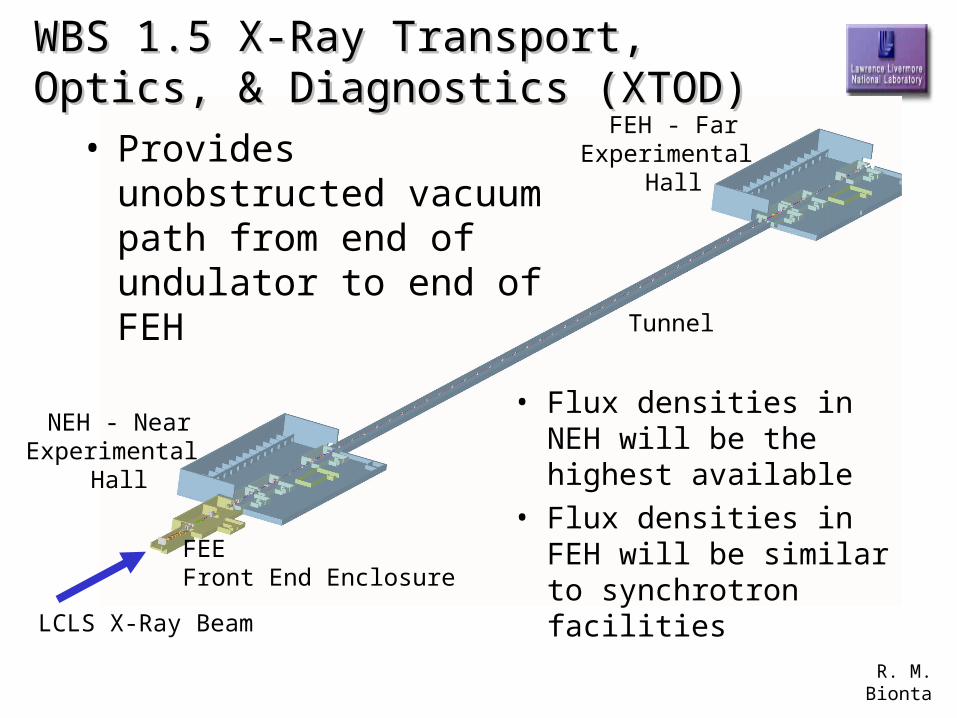
WBS 1.5 X-Ray Transport, Optics, & WBS 1.5 X-Ray Transport, Optics, & Diagnostics (XTOD) Diagnostics (XTOD)

• Provides unobstructed vacuum path from end of undulator to end of FEH

LCLS X-Ray Beam

Tunnel

NEH - NearExperimental

Hall

• Flux densities in NEH will be the highest available

• Flux densities in FEH will be similar to synchrotron facilities

FEEFront End Enclosure

FEH - FarExperimental

Hall

R. M. Bionta

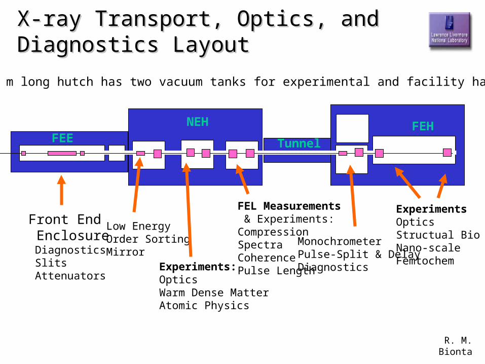
X-ray Transport, Optics, and Diagnostics X-ray Transport, Optics, and Diagnostics LayoutLayout

Front End Enclosure Diagnostics Slits Attenuators

Low EnergyOrder SortingMirror

FEL Measurements & Experiments:CompressionSpectraCoherencePulse Length

MonochrometerPulse-Split & DelayDiagnostics

ExperimentsOpticsStructual BioNano-scaleFemtochem

FEENEH FEH

Tunnel

Experiments:OpticsWarm Dense MatterAtomic Physics

Each 13 m long hutch has two vacuum tanks for experimental and facility hardware

Beam Models

R. M. Bionta

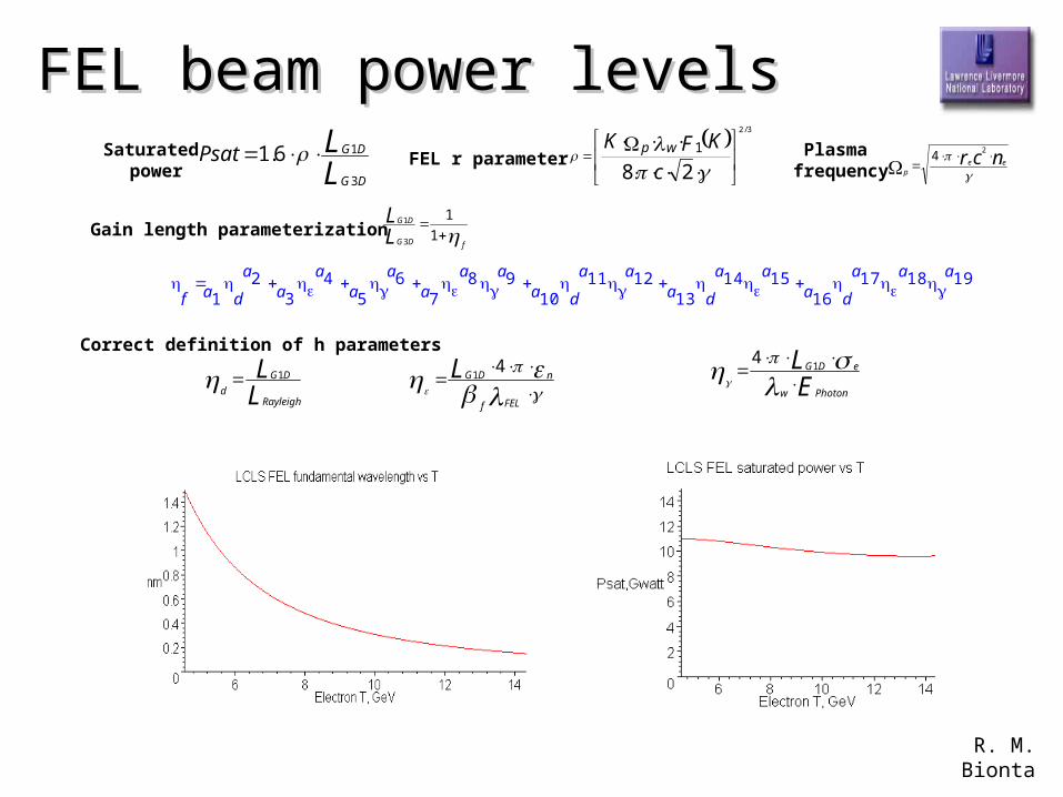
FEL beam power levelsFEL beam power levels

LL

DG

DGPsat3

16.1

28

1

3/2

c

KFK wp

ncr ee

p

24

fDG

DG

LL

1

1

3

1

f

a1d

a2a3

a4

a5a6

a7a8

a9a10

d

a11 a12

a13d

a14 a15

a16d

a17 a18

a19

LLRayleigh

DG

d

1

FELf

nDGL 41

EL

Photonw

eDG

14

Saturated power

FEL r parameter Plasma frequency

Gain length parameterization

Correct definition of h parameters

R. M. Bionta

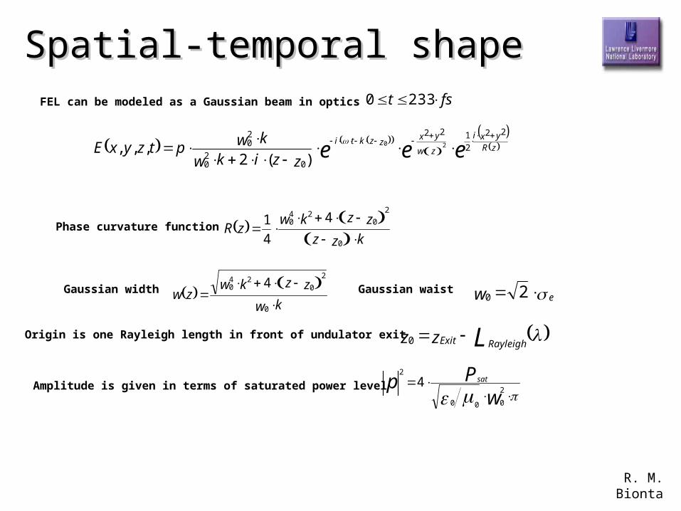
Spatial-temporal shapeSpatial-temporal shape

eee zRyxi

zw

yxzzkti

zzikw

kwptzyxE22

2

122

020

20 20

)(2,,,

kw

zzkwzw

0

0

2240 4

kzz

zzkwzR

0

0

2240 4

4

1

ew 20

LRayleighExitzz 0

wPp sat

2

000

2

4

fst 2330FEL can be modeled as a Gaussian beam in optics

Phase curvature function

Gaussian width Gaussian waist

Origin is one Rayleigh length in front of undulator exit

Amplitude is given in terms of saturated power level

R. M. Bionta

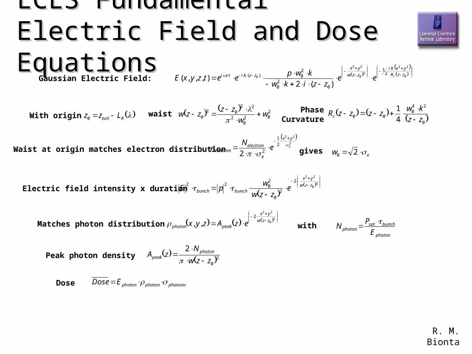
LCLS Fundamental Electric Field LCLS Fundamental Electric Field and Dose Equationsand Dose Equations

0

22

20

22

02

1

020

20)(

)(2),,,( zzR

yxki

zzw

yx

zzkitti ceezzikw

kwpeetzyxE

202

02

2202

0 ww

zzzzw

0

240

00 4

1

zz

kwzzzzRc

2

22

2

1

22e

yx

e

electronelectron e

N

Rexit Lzz 0

ew 20

2

0

22

2

20

2022 zzw

yx

bunchbunch ezzw

wpE

2

0

22

2

,, zzw

yx

peakphoton ezAzyx

20

2

zzw

NzA photon

peak

photon

bunchsatphoton E

PN

photoionphotonphotonEDose

Gaussian Electric Field:

With origin waist PhaseCurvature

Waist at origin matches electron distribution gives

Electric field intensity x duration

Matches photon distribution with

Peak photon density

Dose

R. M. Bionta

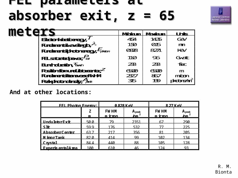
FEL parameters at absorber FEL parameters at absorber exit, z = 65 metersexit, z = 65 meters

Minimum Maximum UnitsElectron kinetic energy, T 4.54 14.35 GeV

Fundamental wavelength, 1.50 0.15 nm

Fundamental photon energy, Ephoton 0.828 8.271 KeV

FEL saturated power, Psat 11.0 9.6 Gwatt

Bunch duration, bunch 233 233 fsec

Position from undulator center, z 65.00 65.00 mFundamental transverse FWHM 232.7 86.7 micron

Peak photon density, Apeak 315 199 photons/nm2

And at other locations:

FEL Photon Energy: 0.828 KeV 8.27 KeVZ FWHM Apeak FWHM Apeak

m micron /nm2 micron /nm2

Undulator Exit 50.0 79 2351 67 290Slit 59.9 176 532 77 225Absorber Center 63.7 217 356 81 205Mirror Tank 82.0 414 99 102 134Crystal 84.4 440 88 105 128Experimental Area 100 610 46 124 93

R. M. Bionta

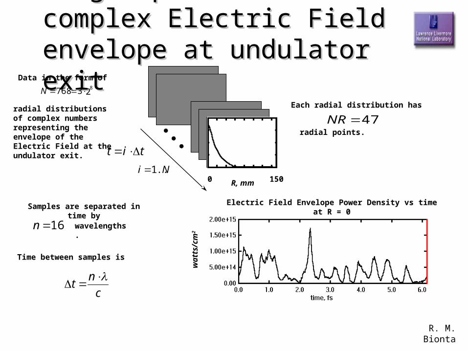
Ginger provides complex Ginger provides complex Electric Field envelope at Electric Field envelope at undulator exitundulator exit

23768 8N

Data in the form of

radial distributionsof complex numbersrepresenting theenvelope of the Electric Field at theundulator exit. tit

c

nt

16n

Samples are separated in time by

wavelengths.

Time between samples is

Ni ..1R, mm0 150

Each radial distribution has

47NRradial points.

Electric Field Envelope Power Density vs timeat R = 0

wa

tts

/cm

2

R. M. Bionta

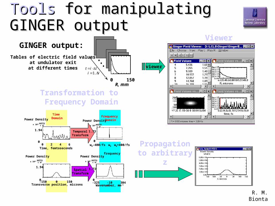
ToolsTools for manipulating GINGER for manipulating GINGER outputoutput

0 150

GINGER output:

Tables of electric field valuesat undulator exitat different times

Time Domain

Frequency Domain

TemporalTransform

SpatialTransform

00

1.94

150-150Transverse position, microns

x 1015 wattsc m2

Power Density

0

1.94

x 1015 wattsc m2

0 6Time, femtoseconds

42

Power Density

0w0w0-400/fs

1.73

x 1017 wattsc m2

w0+400/fs

frequency

Power Density

0-10

1.73

-325 304Wavenumber, mm-1

x 1017 wattsc m2

Power Density

viewer

Viewer

Transformation to Frequency Domain

Propagationto arbitrary

z

tit Ni ..1

R, mm

R. M. Bionta

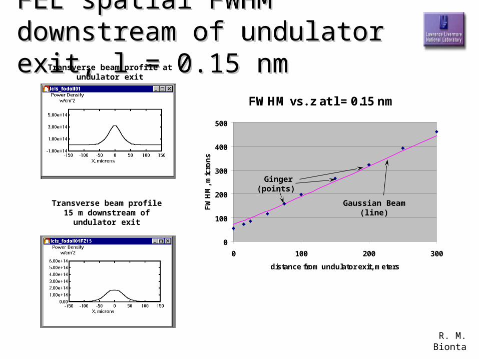
FEL spatial FWHM downstream FEL spatial FWHM downstream of undulator exit, of undulator exit, l l = 0.15 nm= 0.15 nm

Transverse beam profile atundulator exit

Transverse beam profile15 m downstream of

undulator exit

FWHM vs. z at l = 0.15 nm

0

100

200

300

400

500

0 100 200 300

distance from undulator exit, meters

FW

HM

, mic

ron

s

Ginger(points)

Gaussian Beam(line)

R. M. Bionta

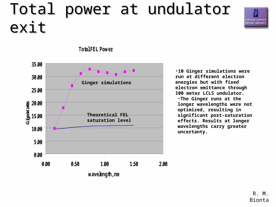
Total power at undulator exitTotal power at undulator exit

Total FEL Power

0.00

5.00

10.00

15.00

20.00

25.00

30.00

35.00

0.00 0.50 1.00 1.50 2.00

wavelength, nm

Gig

a-W

atts

Ginger simulations

Theoretical FEL saturation level

•10 Ginger simulations were run at different electron energies but with fixed electron emittance through 100 meter LCLS undulator.

•The Ginger runs at the longer wavelengths were not optimized, resulting in significant post-saturation effects. Results at longer wavelengths carry greater uncertanty.

R. M. Bionta

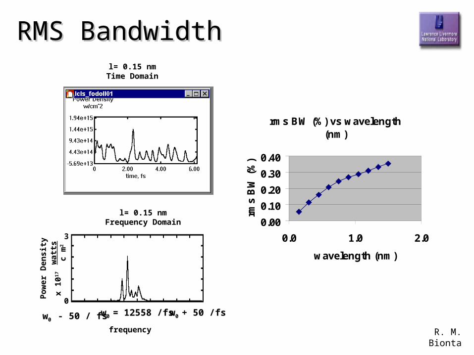
RMS BandwidthRMS Bandwidth

0

w0 = 12558 /fsw0 - 50 / fs

3

x 1

017

w

att

sc

m2

w0 + 50 /fs

frequency

Po

we

r D

en

sit

y

l= 0.15 nmTime Domain

l= 0.15 nmFrequency Domain

rms BW (%) vs wavelength (nm)

0.00

0.10

0.20

0.30

0.40

0.0 1.0 2.0

wavelength (nm)rm

s B

W (

%)

R. M. Bionta

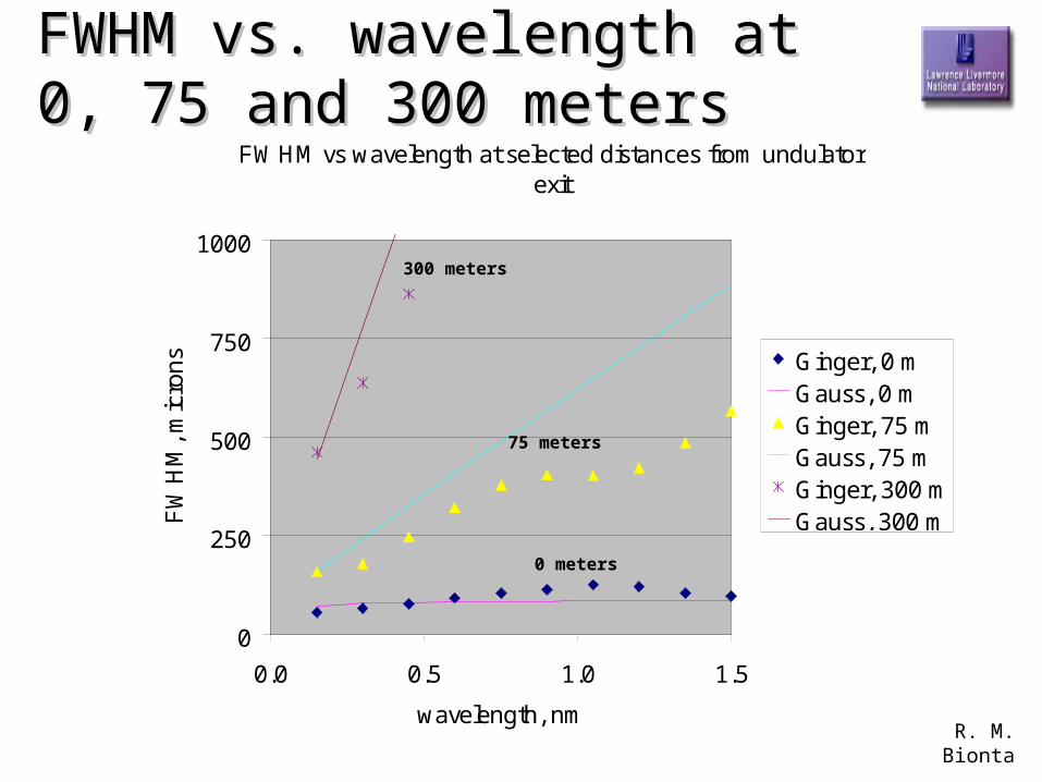
FWHM vs wavelength at selected distances from undulator exit

0

250

500

750

1000

0.0 0.5 1.0 1.5

wavelength, nm

FW

HM

, mic

ron

s Ginger, 0 mGauss, 0 mGinger, 75 mGauss, 75 mGinger, 300 mGauss, 300 m

300 meters

75 meters

0 meters

FWHM vs. wavelength at 0, 75 FWHM vs. wavelength at 0, 75 and 300 metersand 300 meters

R. M. Bionta

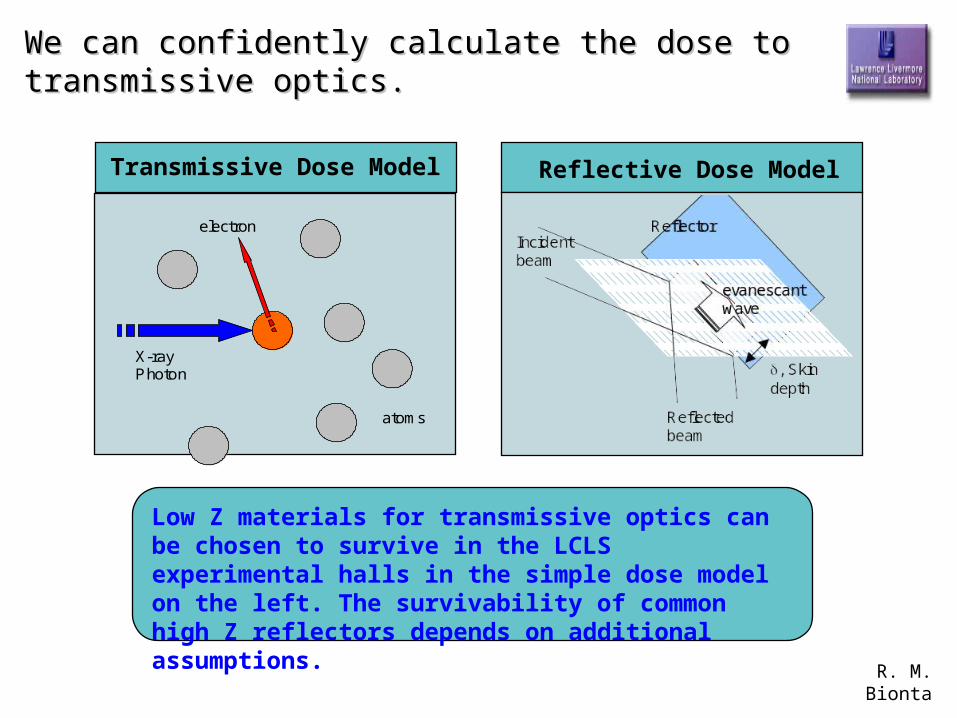
We can confidently calculate the dose to transmissive We can confidently calculate the dose to transmissive optics.optics.

Low Z materials for transmissive optics can be chosen to survive in the LCLS experimental halls in the simple dose model on the left. The survivability of common high Z reflectors depends on additional assumptions.

Transmissive Dose Model

X-ray Photon

electron

atoms

Reflective Dose Model

R. M. Bionta

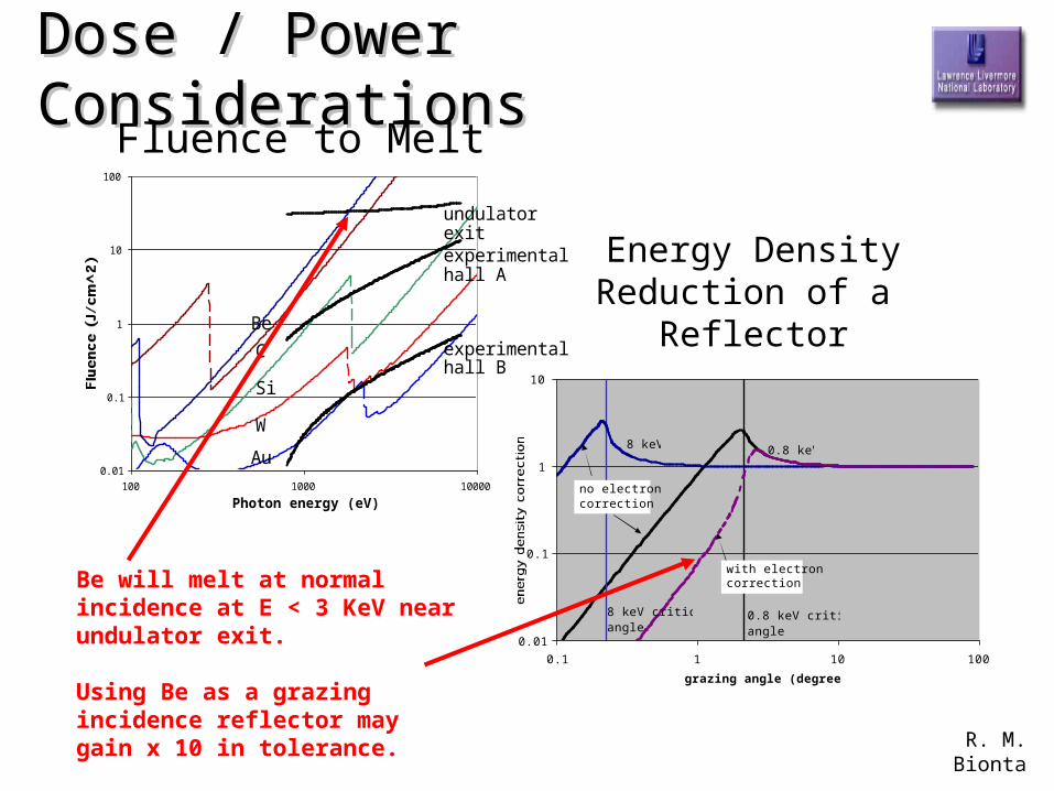
Dose / Power ConsiderationsDose / Power Considerations

0.01

0.1

1

10

100

100 1000 10000

Photon energy (eV)

Flu

en

ce (

J/cm

^2

)

undulatorexitexperimentalhall A

experimentalhall B

C

Si

W

Au

Be

0.01

0.1

1

10

0.1 1 10 100

grazing angle (degrees)

energ

y d

ensit

y c

orr

ect

ion

0.8 keV critical angle

0.8 keV

8 keV critical angle

8 keV

with electroncorrection

no electroncorrection

Fluence to Melt

Energy Density Reduction of a

Reflector

Be will melt at normal incidence at E < 3 KeV near undulator exit.

Using Be as a grazing incidence reflector may gain x 10 in tolerance.

R. M. Bionta

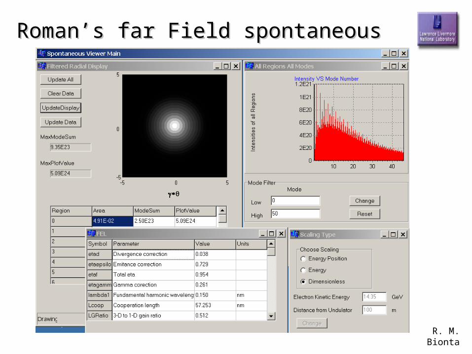
Roman’s far Field spontaneousRoman’s far Field spontaneous

R. M. Bionta

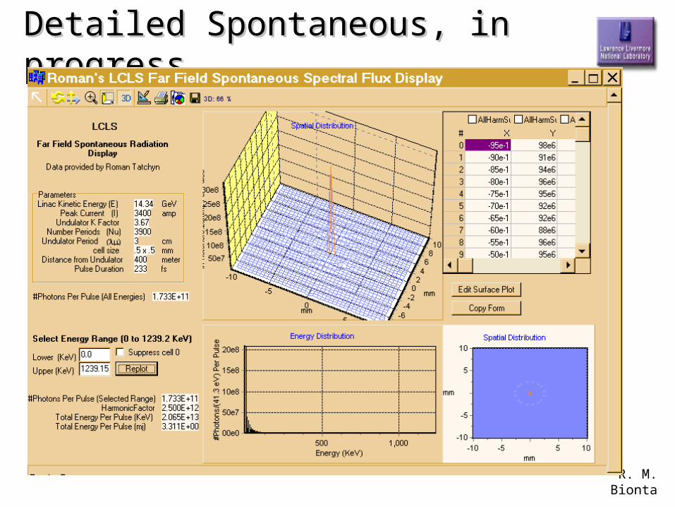
Detailed Spontaneous, in progressDetailed Spontaneous, in progress

R. M. Bionta

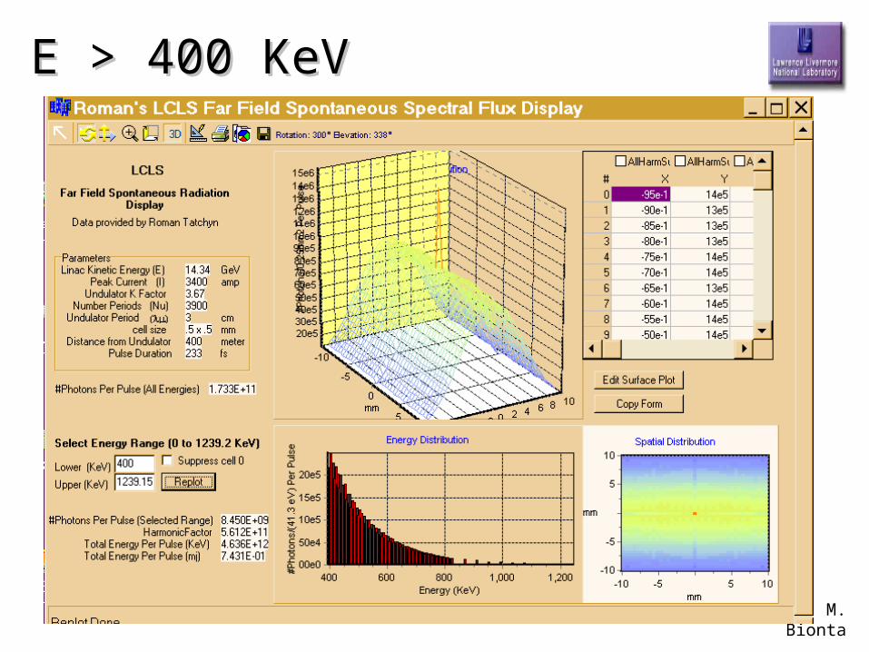
E > 400 KeVE > 400 KeV

R. M. Bionta

FEE InstrumentationFEE Instrumentation

R. M. Bionta

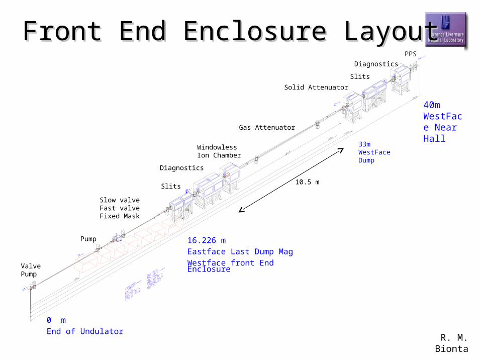
Front End Enclosure LayoutFront End Enclosure Layout

ValvePump

Pump

Slow valveFast valveFixed Mask

Slits

Diagnostics

WindowlessIon Chamber

Gas Attenuator

Solid Attenuator

Slits

Diagnostics

PPS

40mWestFace Near Hall

33mWestFace Dump

16.226 mEastface Last Dump MagWestface front End Enclosure

10.5 m

0 mEnd of Undulator

R. M. Bionta

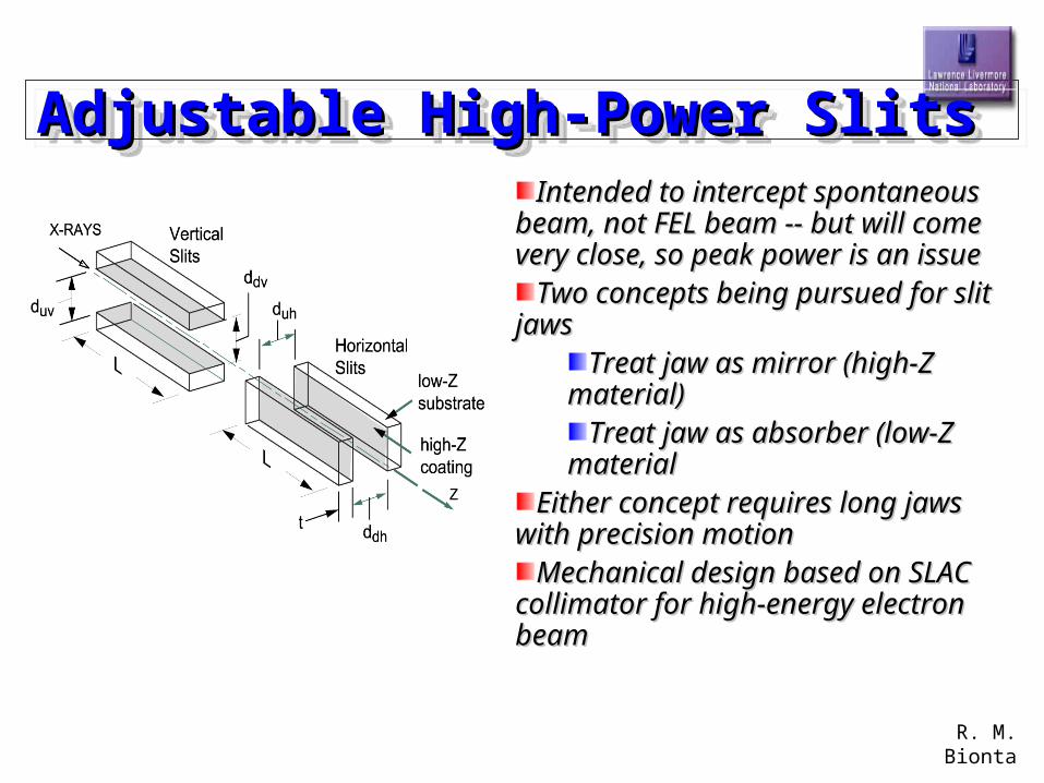
Adjustable High-Power SlitsAdjustable High-Power SlitsAdjustable High-Power SlitsAdjustable High-Power SlitsIntended to intercept Intended to intercept

spontaneous beam, not FEL spontaneous beam, not FEL beam -- but will come very beam -- but will come very close, so peak power is an issueclose, so peak power is an issue

Two concepts being pursued Two concepts being pursued for slit jaws for slit jaws

Treat jaw as mirror (high-Z Treat jaw as mirror (high-Z material)material)

Treat jaw as absorber (low-Treat jaw as absorber (low-Z materialZ material

Either concept requires long Either concept requires long jaws with precision motionjaws with precision motion

Mechanical design based on Mechanical design based on SLAC collimator for high-energy SLAC collimator for high-energy electron beamelectron beam

R. M. Bionta

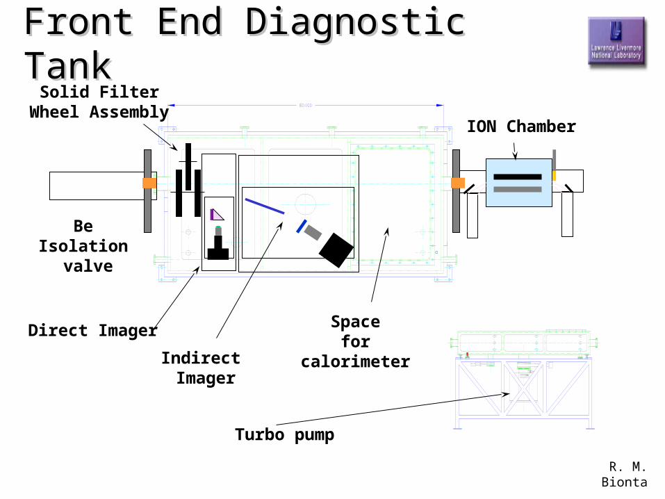
Front End Diagnostic TankFront End Diagnostic Tank

Direct Imager

Indirect Imager

ION Chamber

Turbo pump

Space for

calorimeter

BeIsolation

valve

Solid Filter Wheel Assembly

R. M. Bionta

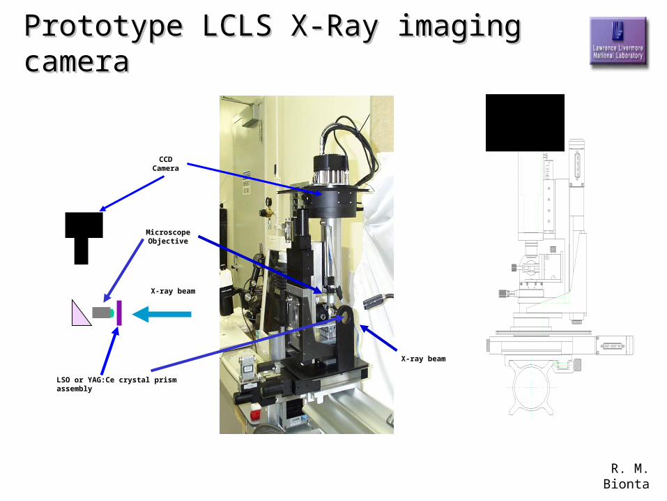
Prototype LCLS X-Ray imaging cameraPrototype LCLS X-Ray imaging camera

CCDCamera

MicroscopeObjective

LSO or YAG:Ce crystal prism assembly

X-ray beam

X-ray beam

R. M. Bionta

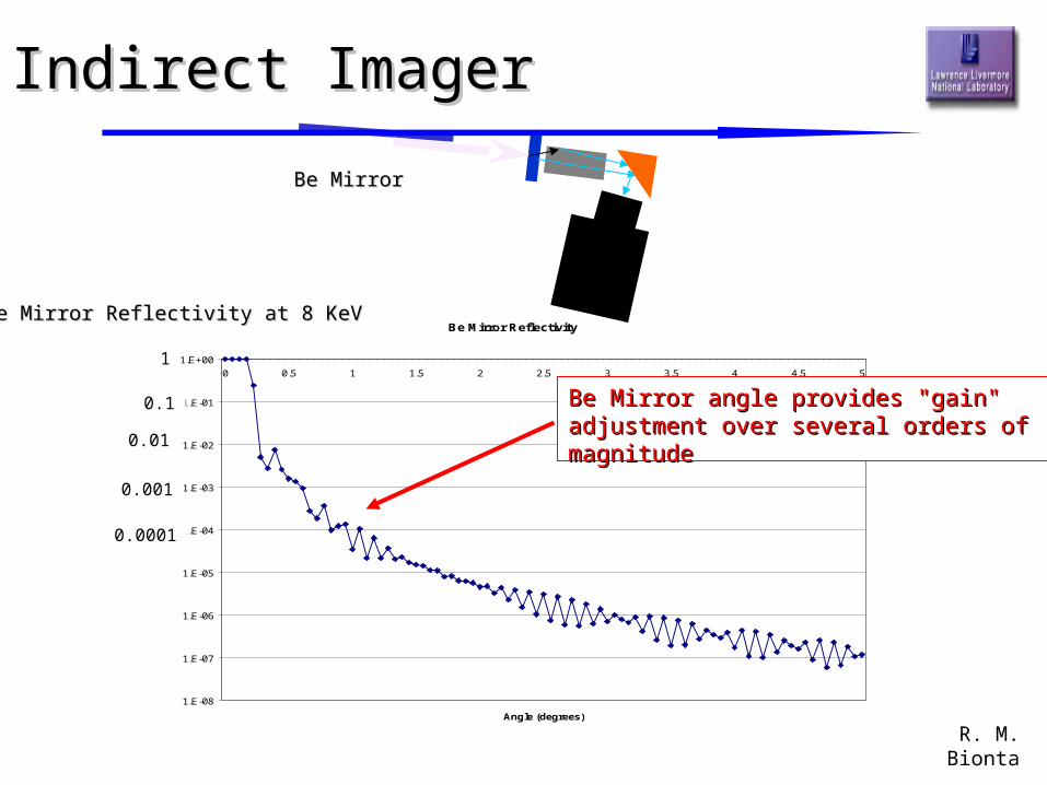
Be Mirror Reflectivity

1.E-08

1.E-07

1.E-06

1.E-05

1.E-04

1.E-03

1.E-02

1.E-01

1.E+00

0 0.5 1 1.5 2 2.5 3 3.5 4 4.5 5

Angle (degrees)

R

Indirect ImagerIndirect Imager

Be Mirror Reflectivity at 8 KeVBe Mirror Reflectivity at 8 KeV

1

0.1

0.01

0.001

0.0001

Be MirrorBe Mirror

Be Mirror angle provides "gain" adjustment Be Mirror angle provides "gain" adjustment over several orders of magnitudeover several orders of magnitude

R. M. Bionta

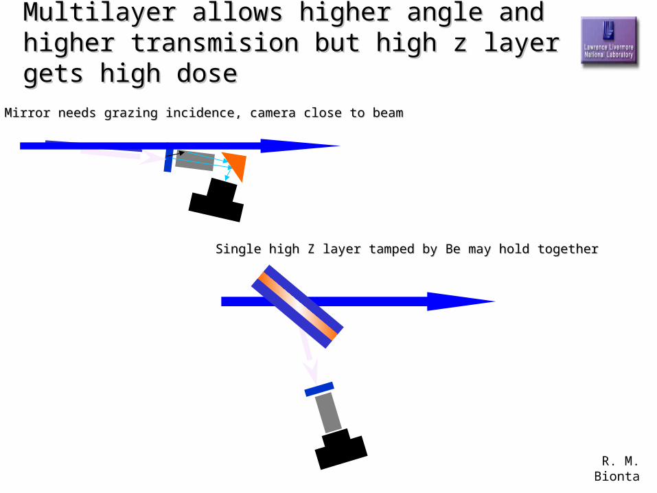
Multilayer allows higher angle and higher Multilayer allows higher angle and higher transmision but high z layer gets high dosetransmision but high z layer gets high dose

Be Mirror needs grazing incidence, camera close to beamBe Mirror needs grazing incidence, camera close to beam

Single high Z layer tamped by Be may hold togetherSingle high Z layer tamped by Be may hold together

R. M. Bionta

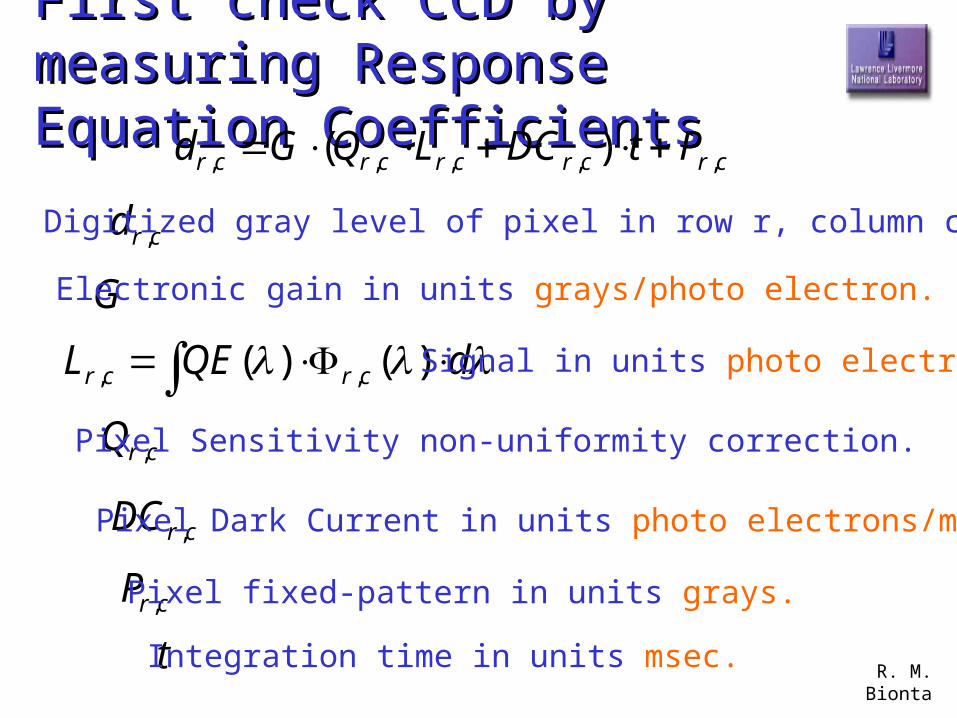
First check CCD by measuring First check CCD by measuring Response Equation CoefficientsResponse Equation Coefficients

crcrcrcrcr PtDCLQGd ,,,,, )(

crd ,

G

dQEL crcr )()( ,,

crDC ,

crQ ,

crP ,

t

Digitized gray level of pixel in row r, column c.

Electronic gain in units grays/photo electron.

Signal in units photo electrons.

Pixel Sensitivity non-uniformity correction.

Pixel Dark Current in units photo electrons/msec.

Pixel fixed-pattern in units grays.

Integration time in units msec.

R. M. Bionta

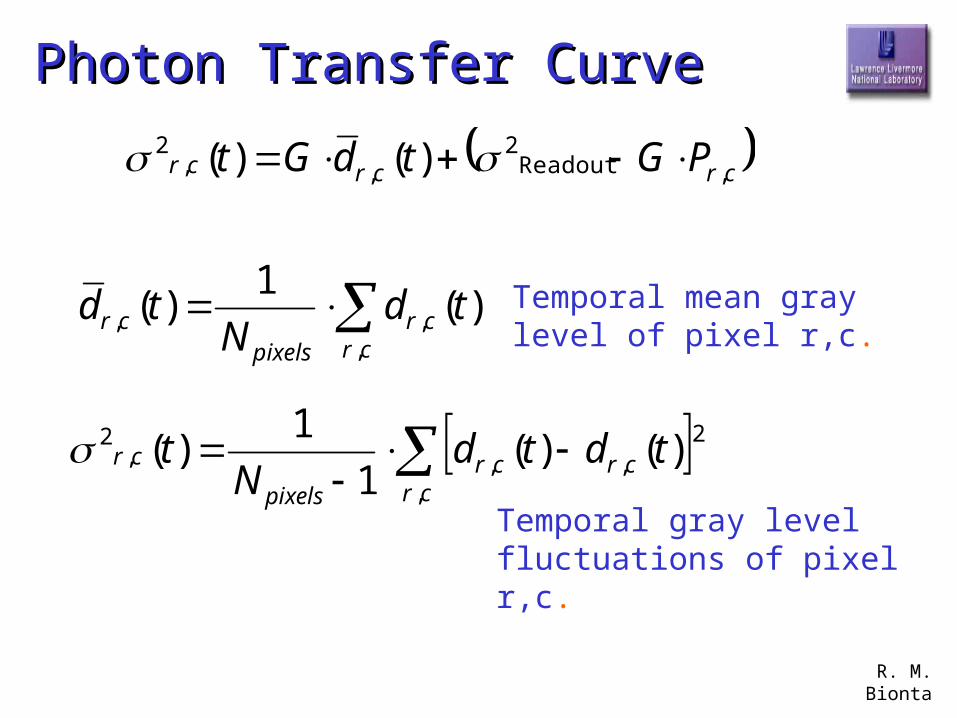
Photon Transfer CurvePhoton Transfer Curve

crcrcr PGtdGt ,Readout2

,,2 )()(

cr

crpixels

cr tdN

td,

,, )(1

)( Temporal mean gray level of pixel r,c.

cr

crcrpixels

cr tdtdN

t,

2,,,

2 )()(1

1)(

Temporal gray level fluctuations of pixel r,c.

R. M. Bionta

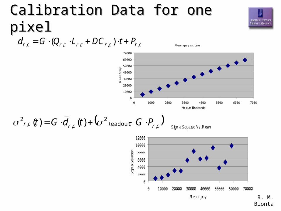
Calibration Data for one pixelCalibration Data for one pixel

Sigma Squared Vs. Mean

0

2000

4000

6000

8000

10000

12000

0 10000 20000 30000 40000 50000 60000 70000

Mean gray

Sigm

a Sq

uare

d

Mean gray vs. time

0

10000

20000

30000

40000

50000

60000

70000

0 1000 2000 3000 4000 5000 6000 7000

time, milliseconds

Me

an

Gra

y

crcrcr PGtdGt ,Readout2

,,2 )()(

crcrcrcrcr PtDCLQGd ,,,,, )(

R. M. Bionta

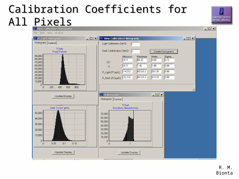
Calibration Coefficients for All PixelsCalibration Coefficients for All Pixels

R. M. Bionta

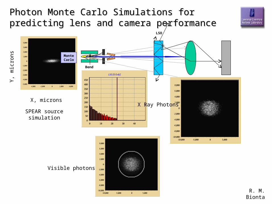
Photon Monte Carlo Simulations for predicting lens and Photon Monte Carlo Simulations for predicting lens and camera performancecamera performance

4,0002,0000-2,000-4,000

4,000

3,000

2,000

1,000

0

-1,000

-2,000

-3,000

-4,000

-5,000

SPEAR source simulation

Visible photons

X, microns

Y, m

icro

ns

LSO25 Exit Z

403020100

450

400

350

300

250

200

150

100

50

0

MonteCarlo

Bend

LSO

5,0000-5,000-10,000

8,000

6,000

4,000

2,000

0

-2,000

-4,000

-6,000

-8,000

-10,000

5,0000-5,000-10,000

8,000

6,000

4,000

2,000

0

-2,000

-4,000

-6,000

-8,000

-10,000

X Ray Photons

R. M. Bionta

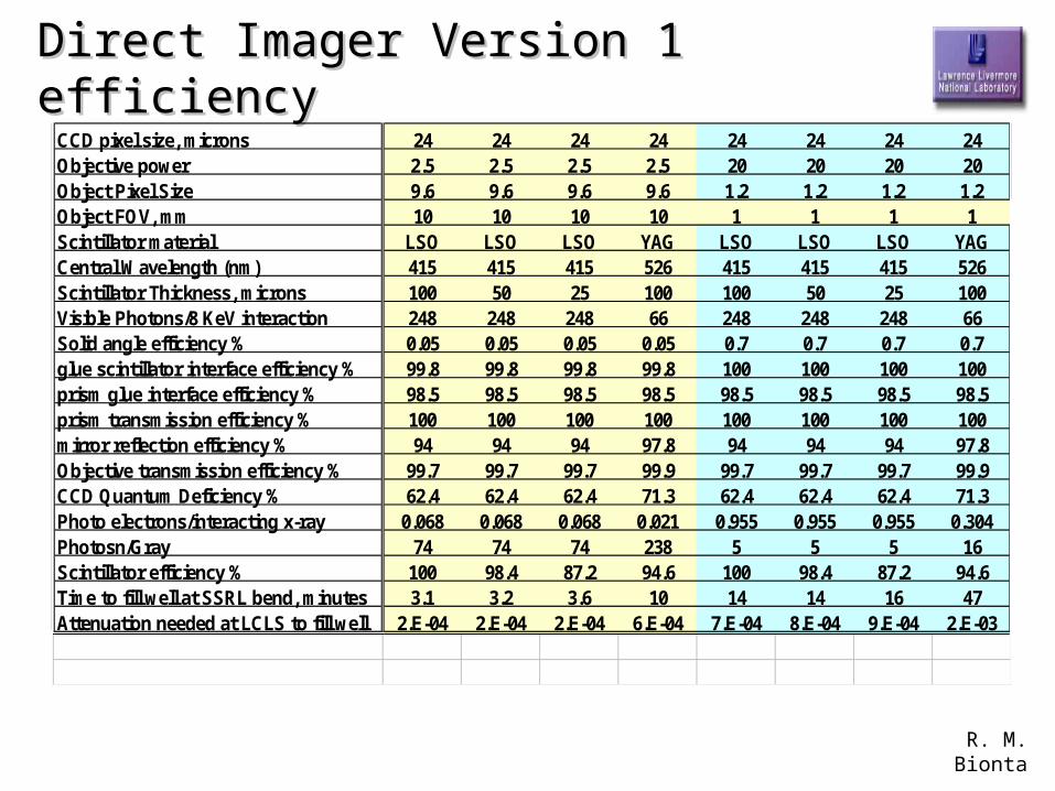
Direct Imager Version 1 efficiencyDirect Imager Version 1 efficiencyCCD pixel size, microns 24 24 24 24 24 24 24 24Objective power 2.5 2.5 2.5 2.5 20 20 20 20Object Pixel Size 9.6 9.6 9.6 9.6 1.2 1.2 1.2 1.2Object FOV, mm 10 10 10 10 1 1 1 1Scintillator material LSO LSO LSO YAG LSO LSO LSO YAGCentral Wavelength (nm) 415 415 415 526 415 415 415 526Scintillator Thickness, microns 100 50 25 100 100 50 25 100Visible Photons/8 KeV interaction 248 248 248 66 248 248 248 66Solid angle efficiency % 0.05 0.05 0.05 0.05 0.7 0.7 0.7 0.7glue scintillator interface efficiency % 99.8 99.8 99.8 99.8 100 100 100 100prism glue interface efficiency % 98.5 98.5 98.5 98.5 98.5 98.5 98.5 98.5prism transmission efficiency % 100 100 100 100 100 100 100 100mirror reflection efficiency % 94 94 94 97.8 94 94 94 97.8Objective transmission efficiency % 99.7 99.7 99.7 99.9 99.7 99.7 99.7 99.9CCD Quantum Deficiency % 62.4 62.4 62.4 71.3 62.4 62.4 62.4 71.3Photo electrons/interacting x-ray 0.068 0.068 0.068 0.021 0.955 0.955 0.955 0.304Photosn/Gray 74 74 74 238 5 5 5 16Scintillator efficiency % 100 98.4 87.2 94.6 100 98.4 87.2 94.6Time to fill well at SSRL bend, minutes 3.1 3.2 3.6 10 14 14 16 47Attenuation needed at LCLS to fill well 2.E-04 2.E-04 2.E-04 6.E-04 7.E-04 8.E-04 9.E-04 2.E-03

R. M. Bionta

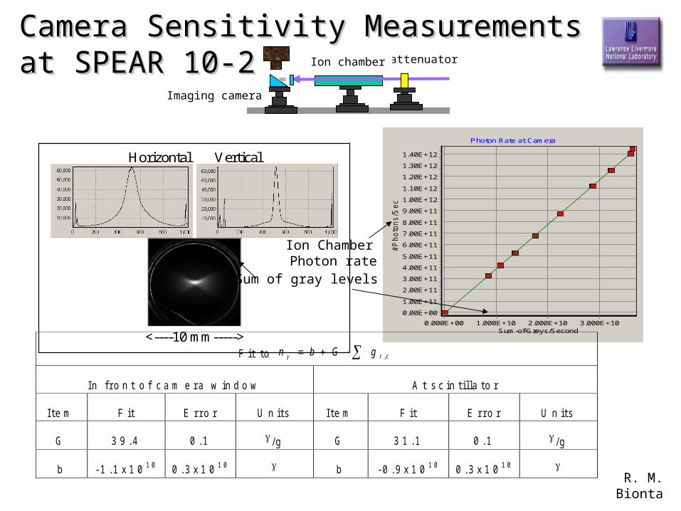
Camera Sensitivity Measurements at Camera Sensitivity Measurements at SPEAR 10-2SPEAR 10-2

Horizontal Vertical

<----10 mm----->

Photon Rate at Camera

Sum-of-Greys/Second3.000E+102.000E+101.000E+100.000E+00

#P

hoto

ns/S

ec

1.40E+12

1.30E+12

1.20E+12

1.10E+12

1.00E+12

9.00E+11

8.00E+11

7.00E+11

6.00E+11

5.00E+11

4.00E+11

3.00E+11

2.00E+11

1.00E+11

0.00E+00

F i t t o crgGbn ,

I n f r o n t o f c a m e r a w i n d o w A t s c i n t i l l a t o r

I t e m F i t E r r o r U n i t s I t e m F i t E r r o r U n i t s

G 3 9 . 4 0 . 1 / g G 3 1 . 1 0 . 1 / g

b - 1 . 1 x 1 0 1 0 0 . 3 x 1 0 1 0 b - 0 . 9 x 1 0 1 0 0 . 3 x 1 0 1 0

Sum of gray levels

Ion Chamber Photon rate

attenuator

Imaging camera

Ion chamber

R. M. Bionta

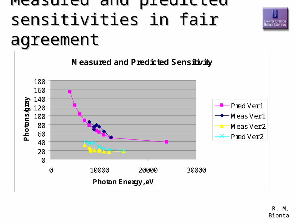
Measured and predicted Measured and predicted sensitivities in fair agreementsensitivities in fair agreement

Measured and Predicted Sensitivity

020406080

100120140160180

0 10000 20000 30000

Photon Energy, eV

Ph

oto

ns/g

ray

Pred Ver 1

Meas Ver 1

Meas Ver 2

Pred Ver 2

R. M. Bionta

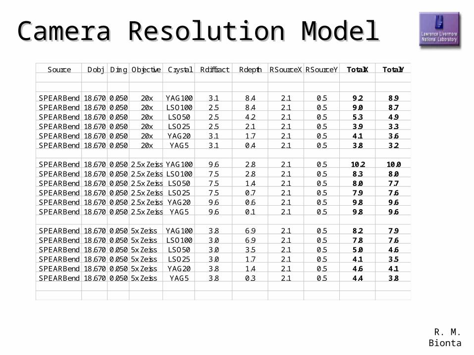
Camera Resolution ModelCamera Resolution ModelSource Dobj Dimg Objective Crystal Rdiffract Rdepth RSourceX RSourceY TotalX TotalY

SPEARBend 18.670 0.050 20x YAG100 3.1 8.4 2.1 0.5 9.2 8.9SPEARBend 18.670 0.050 20x LSO100 2.5 8.4 2.1 0.5 9.0 8.7SPEARBend 18.670 0.050 20x LSO50 2.5 4.2 2.1 0.5 5.3 4.9SPEARBend 18.670 0.050 20x LSO25 2.5 2.1 2.1 0.5 3.9 3.3SPEARBend 18.670 0.050 20x YAG20 3.1 1.7 2.1 0.5 4.1 3.6SPEARBend 18.670 0.050 20x YAG5 3.1 0.4 2.1 0.5 3.8 3.2

SPEARBend 18.670 0.050 2.5x Zeiss YAG100 9.6 2.8 2.1 0.5 10.2 10.0SPEARBend 18.670 0.050 2.5x Zeiss LSO100 7.5 2.8 2.1 0.5 8.3 8.0SPEARBend 18.670 0.050 2.5x Zeiss LSO50 7.5 1.4 2.1 0.5 8.0 7.7SPEARBend 18.670 0.050 2.5x Zeiss LSO25 7.5 0.7 2.1 0.5 7.9 7.6SPEARBend 18.670 0.050 2.5x Zeiss YAG20 9.6 0.6 2.1 0.5 9.8 9.6SPEARBend 18.670 0.050 2.5x Zeiss YAG5 9.6 0.1 2.1 0.5 9.8 9.6

SPEARBend 18.670 0.050 5x Zeiss YAG100 3.8 6.9 2.1 0.5 8.2 7.9SPEARBend 18.670 0.050 5x Zeiss LSO100 3.0 6.9 2.1 0.5 7.8 7.6SPEARBend 18.670 0.050 5x Zeiss LSO50 3.0 3.5 2.1 0.5 5.0 4.6SPEARBend 18.670 0.050 5x Zeiss LSO25 3.0 1.7 2.1 0.5 4.1 3.5SPEARBend 18.670 0.050 5x Zeiss YAG20 3.8 1.4 2.1 0.5 4.6 4.1SPEARBend 18.670 0.050 5x Zeiss YAG5 3.8 0.3 2.1 0.5 4.4 3.8

R. M. Bionta

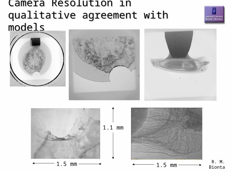
Camera Resolution in qualitative Camera Resolution in qualitative agreement with modelsagreement with models

1.5 mm

1.1 mm

1.5 mm

R. M. Bionta

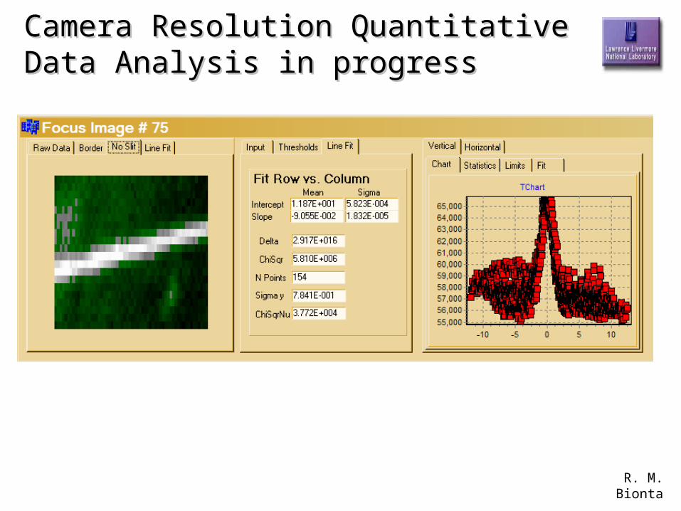
Camera Resolution Quantitative Data Camera Resolution Quantitative Data Analysis in progressAnalysis in progress

R. M. Bionta

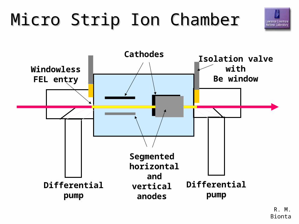
Micro Strip Ion ChamberMicro Strip Ion Chamber

Differentialpump

Differentialpump

Cathodes

Segmented horizontal

and vertical anodes

Isolation valve with

Be windowWindowless

FEL entry

R. M. Bionta

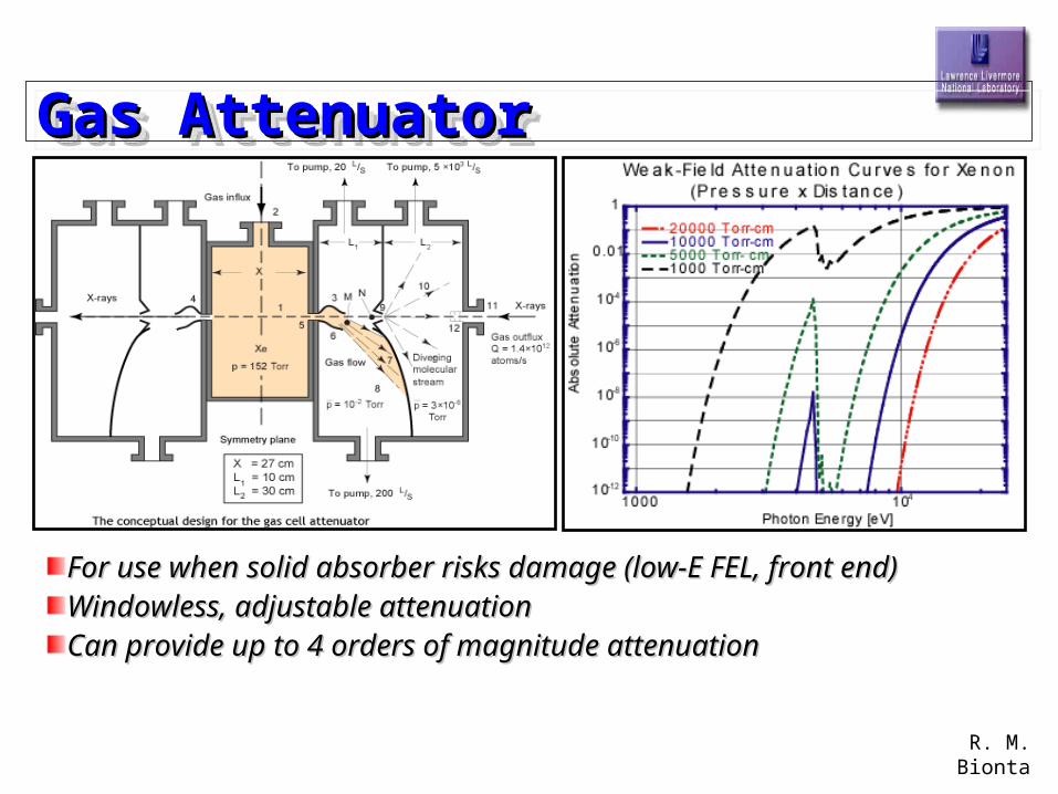
Gas AttenuatorGas AttenuatorGas AttenuatorGas Attenuator

For use when solid absorber risks damage (low-E FEL, front end)For use when solid absorber risks damage (low-E FEL, front end)Windowless, adjustable attenuationWindowless, adjustable attenuationCan provide up to 4 orders of magnitude attenuationCan provide up to 4 orders of magnitude attenuation

R. M. Bionta

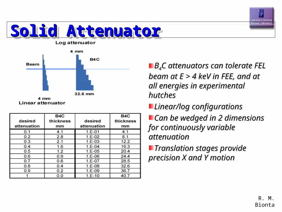
Solid AttenuatorSolid AttenuatorSolid AttenuatorSolid Attenuator

BB44C attenuators can tolerate C attenuators can tolerate FEL beam at E > 4 keV in FEL beam at E > 4 keV in FEE, and at all energies in FEE, and at all energies in experimental hutchesexperimental hutches

Linear/log configurationsLinear/log configurations

Can be wedged in 2 Can be wedged in 2 dimensions for continuously dimensions for continuously variable attenuationvariable attenuation

Translation stages provide Translation stages provide precision X and Y motionprecision X and Y motion

R. M. Bionta

MissingMissing

• Predicted performance of direct and indirect imager for Spontanous vs. I, and FEL vs. Power

• Calculations of linearity and signal levels in Ion chamber

• Integration with FEE + Beam Dump floor plan

R. M. Bionta

Commissioning Diagnostic TankCommissioning Diagnostic Tank

R. M. Bionta

Commissioning DiagnosticsCommissioning Diagnostics

Measurements– Total energy– Pulse length– Photon energy spectra– Spatial coherence– Spatial shape and centroid– Divergence

R. M. Bionta

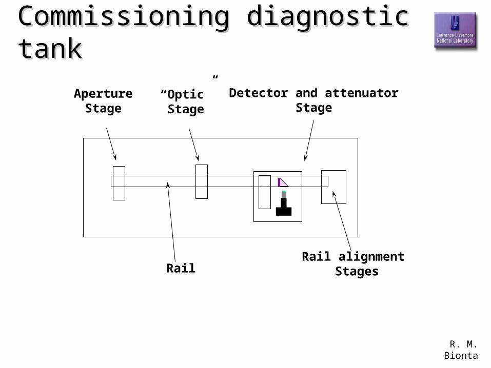
Commissioning diagnostic tankCommissioning diagnostic tank

ApertureStage

“Optic”Stage

Detector and attenuatorStage

Rail alignment StagesRail

R. M. Bionta

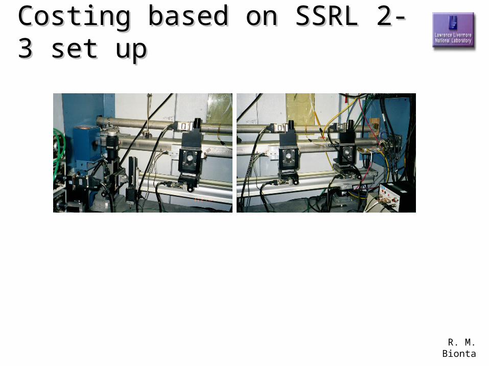
Costing based on SSRL 2-3 set Costing based on SSRL 2-3 set upup

R. M. Bionta

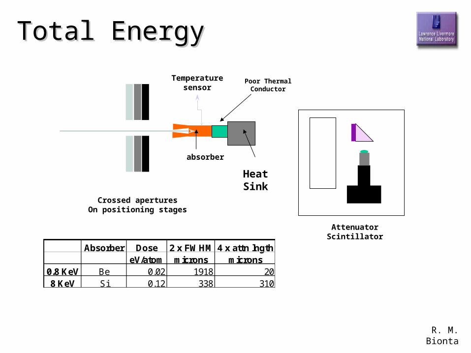
Total EnergyTotal Energy

Crossed aperturesOn positioning stages

absorber

Temperaturesensor

AttenuatorScintillator

Absorber Dose 2 x FWHM 4 x attn lngtheV/atom microns microns

0.8 KeV Be 0.02 1918 208 KeV Si 0.12 338 310

Poor ThermalConductor

HeatSink

R. M. Bionta

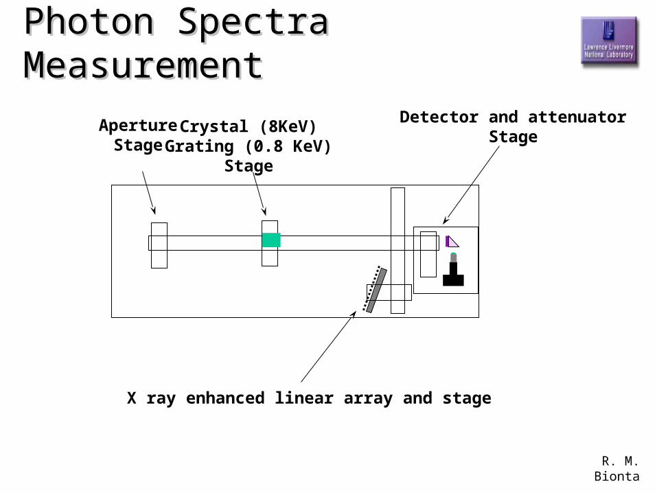
Photon Spectra MeasurementPhoton Spectra Measurement

ApertureStage

Crystal (8KeV)Grating (0.8 KeV)

Stage

Detector and attenuatorStage

X ray enhanced linear array and stage

R. M. Bionta

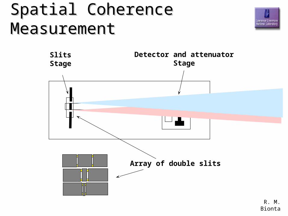
Spatial Coherence MeasurementSpatial Coherence Measurement

SlitsStage

Detector and attenuatorStage

Array of double slits

R. M. Bionta

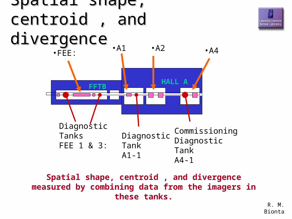
Spatial shape, centroid , and Spatial shape, centroid , and divergencedivergence

•FEE:•A1 •A2 •A4

FFTBHALL A

DiagnosticTanksFEE 1 & 3:

DiagnosticTankA1-1

CommissioningDiagnosticTankA4-1

Spatial shape, centroid , and divergence measured by combining data from the imagers in these tanks.

R. M. Bionta

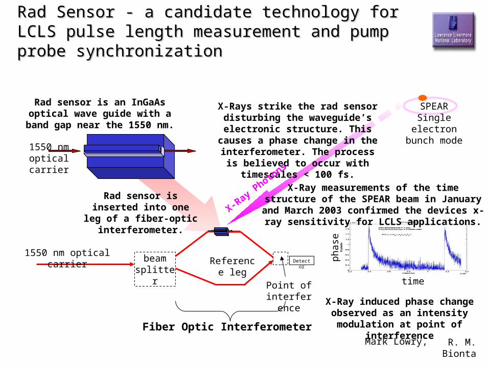
Rad Sensor - a candidate technology for LCLS pulse Rad Sensor - a candidate technology for LCLS pulse length measurement and pump probe synchronizationlength measurement and pump probe synchronization

Rad sensor is an InGaAs optical wave guide with a band gap near the 1550

nm.

1550 nm optical carrier

Reference leg

Detectorbeam splitter

1550 nm optical carrier

Fiber Optic Interferometer

Rad sensor is inserted into one leg of a fiber-optic

interferometer.

X-Rays strike the rad sensor disturbing the waveguide’s electronic structure.

This causes a phase change in the interferometer. The process is believed

to occur with timescales < 100 fs.

X-Ray Photons

Point of interference X-Ray induced phase change observed as

an intensity modulation at point of interference

X-Ray measurements of the time structure of the SPEAR beam in January and March 2003 confirmed the devices x-ray sensitivity for LCLS applications.

time

phas

e

SPEARSingle electron

bunch mode

Mark Lowry,

R. M. Bionta

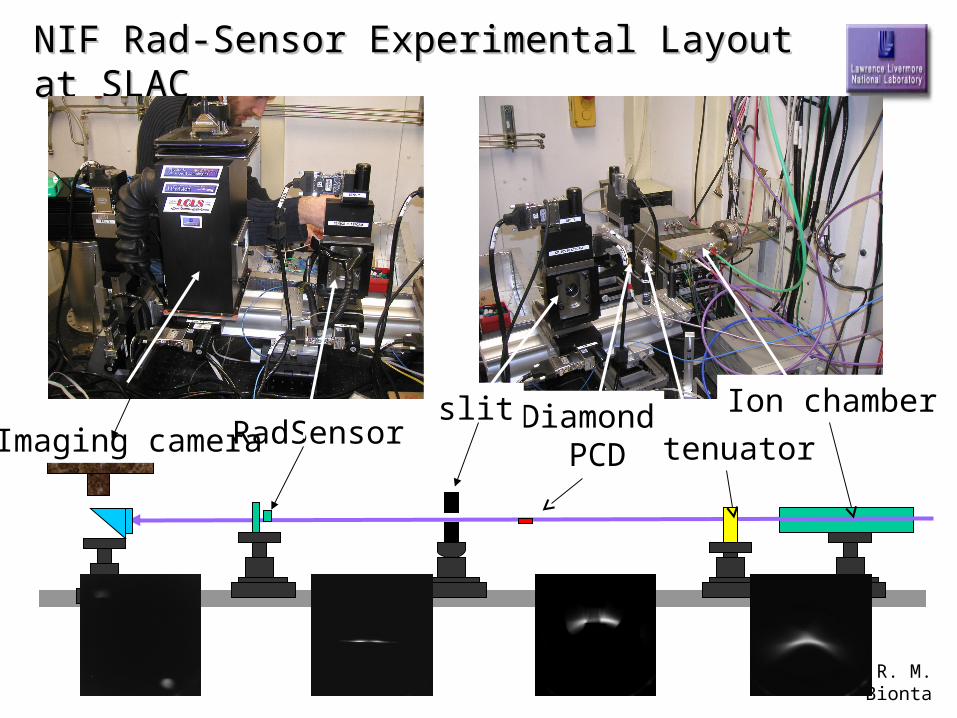
NIF Rad-Sensor Experimental Layout at SLACNIF Rad-Sensor Experimental Layout at SLAC

Ion chamber

attenuatorImaging cameraDiamond

PCDRadSensor

slit

R. M. Bionta

RadSensor Response to single-bucket fill pattern

•Fast rise•Long fall-time will be improved•Complementary outputs =>

•index modulation

Xray pulse history (conventional)

781 ns

Mark Lowry

R. M. Bionta

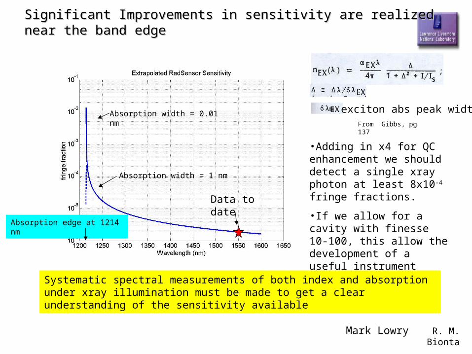
Significant Improvements in sensitivity are realized near the band edgeSignificant Improvements in sensitivity are realized near the band edge

Systematic spectral measurements of both index and absorption under xray illumination must be made to get a clear understanding of the sensitivity available

Absorption width = 0.01 nm

Absorption width = 1 nm

•Adding in x4 for QC enhancement we should detect a single xray photon at least 8x10-4 fringe fractions.

•If we allow for a cavity with finesse 10-100, this allow the development of a useful instrument

Data to date

= exciton abs peak widthFrom Gibbs, pg 137

Absorption edge at 1214 nm

Mark Lowry

R. M. Bionta

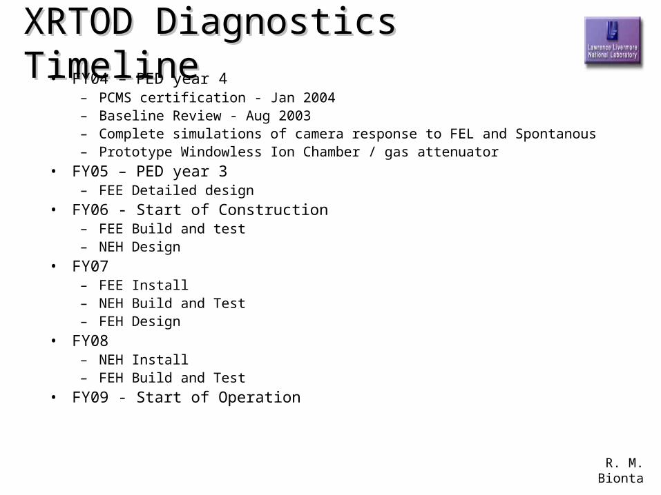
XRTOD Diagnostics TimelineXRTOD Diagnostics Timeline• FY04 – PED year 4

– PCMS certification - Jan 2004– Baseline Review - Aug 2003– Complete simulations of camera response to FEL and Spontanous– Prototype Windowless Ion Chamber / gas attenuator

• FY05 – PED year 3– FEE Detailed design

• FY06 - Start of Construction– FEE Build and test– NEH Design

• FY07– FEE Install– NEH Build and Test– FEH Design

• FY08– NEH Install– FEH Build and Test

• FY09 - Start of Operation

R. M. Bionta

Startup ProcedureStartup Procedure

R. M. Bionta

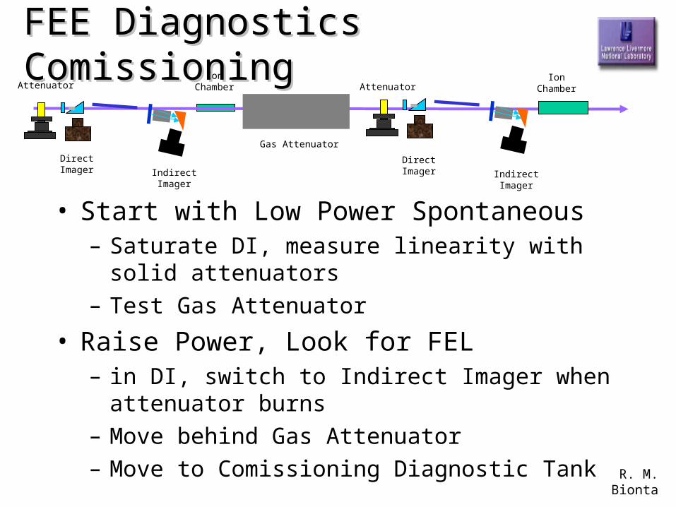
FEE Diagnostics ComissioningFEE Diagnostics Comissioning

• Start with Low Power Spontaneous– Saturate DI, measure linearity with solid

attenuators– Test Gas Attenuator

• Raise Power, Look for FEL– in DI, switch to Indirect Imager when attenuator

burns– Move behind Gas Attenuator– Move to Comissioning Diagnostic Tank

Attenuator

DirectImager Indirect

Imager

IonChamber Attenuator

DirectImager Indirect

Imager

IonChamber

Gas Attenuator

R. M. Bionta

SummarySummary

• 3 detector designs for flexibility

• Move back if necessary

• Bring on the beam!