XnODR and XnIDR: Two Accurate and Fast Fully Connected LayersFor Convolutional Neural NetworksJian Suna, Ali Pourramezan Fardb and Mohammad H. Mahoorb

aDepartment Of Computer Science, University of Denver, 2155 E Wesley Ave, Denver, 80210, Colorado, USAbDepartment Of Computer Engineering, University of Denver, 2155 E Wesley Ave, Denver, 80210, Colorado, USA

A R T I C L E I N F O

Keywords:CapsNetXNOR-NetDynamic RoutingBinarizationXnorizationMachine LearningNeural Network

A B S T R A C T

Although Capsule Networks show great abilities in defining the position relationship between featuresin deep neural networks for visual recognition tasks, they are computationally expensive and notsuitable for running on mobile devices. The bottleneck is in the computational complexity of theDynamic Routing mechanism used between capsules. On the other hand, neural networks such asXNOR-Net are fast and computationally efficient but have relatively low accuracy because of theirinformation loss in the binarization process. This paper proposes a new class of Fully Connected(FC) Layers by xnorizing the linear projector outside or inside the Dynamic Routing within CapsFClayer. Specifically, our proposed FC layers has two versions, XnODR (Xnorizing Linear ProjectorOutside Dynamic Routing) and XnIDR (Xnorizing Linear Projector Inside Dynamic Routing). Totest their generalization, we insert them into MobileNet V2 and ResNet-50 separately. Experimentson three datasets, MNIST, CIFAR-10, MultiMNIST validate their effectiveness. Our experimentalresults demonstrate that both XnODR and XnIDR help networks to have high accuracy with lowerFLOPs and fewer parameters (e.g., 95.32% accuracy with 2.99M parameters and 311.22M FLOPs onCIFAR-10).

1. IntroductionWith the advancement of new computing devices, Con-

volution - based Neural Networks (CNNs) show dominancein image classification due to the CNNs’ powerful and effi-cient feature extraction ability. Despite their power, CNNshave some limitations in capturing the positional relationbetween features in images. For example, a face with ran-domly ordered eyes, ears, nose, mouth, and eyebrows willbe wrongly recognized as a human face.

To address this problem, Sabour et al. proposed Cap-suleNet (CapsNet) in 2017 [34]. They introduced a newconcept called Capsule, a group of neurons whose activityvector represents the instantiation parameters of a specifictype of entity such as an object or an object part. Inbetter words, a capsule is a vector, where its length sizemeans the possibility of the appearance of an object oran image property. Its direction represents the object’simage property, such as location, shape, size, direction, etc.Capsule’s direction is mutually exclusive to its length. Todeploy Capsule, Sabour et al. took the idea of K-Meansclustering, created a Dynamic Routing (DR) mechanism asthe classifier, embedded it into the network’s final FC layer,and called this new layer CapsFC layer.

The CapsFC layer contains the linear projector and theDR mechanism. It loads input capsules into linear projectorfirstly, then improves the accuracy by DR, an iterativestructure (check Section 3.1 for more details about DynamicRouting). The linear projector outside the DR mechanismtakes 5-dimensional capsules as input variables, while the

Jian.Sun86@du.edu (J. Sun);Ali.Pourramezanfard@du.edu (A.P. Fard); mmahoor@du.edu(M.H. Mahoor)

ORCID(s): 0000-0002-9367-0892 (J. Sun)

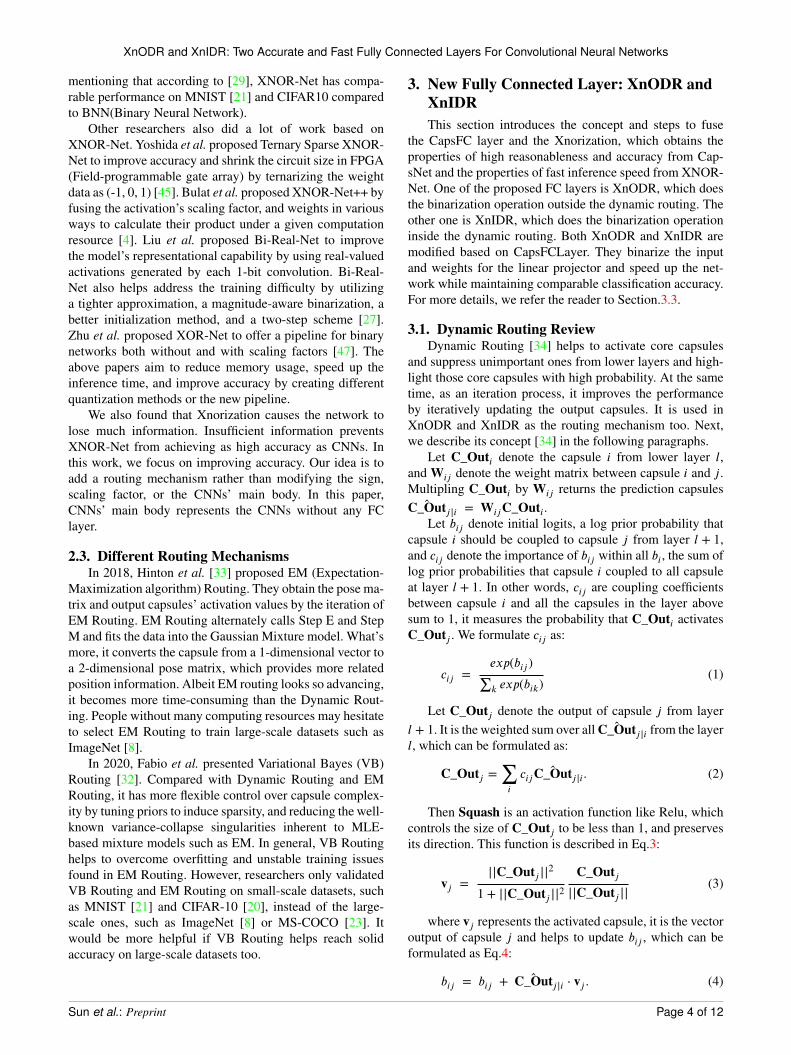
Figure 1: XnIDR(Xnor Inside Dynamic Routing), the Version2 of proposed Fully Connected layer.

usual linear projector only accepts 2-dimensional flattentensors. Dimension expansion causes the surge of param-eters, multiplication and addition (MADD [35]) operations,and processing time. So does iteration. Therefore, comparedwith the usual FC layers, the CapsFC layer decreases thespeed of both training and inference due to the dimensionexpansion and iterative structure. On the other hand, thelightweight models spend less time on network training and

Sun et al.: Preprint Page 1 of 12

arX

iv:2

111.

1085

4v1

[cs

.CV

] 2

1 N

ov 2

021

XnODR and XnIDR: Two Accurate and Fast Fully Connected Layers For Convolutional Neural Networks

inference but perform as well as CapsNet. For example,Section.4 presents that MobileNet V2 [35] achieves 99.50%accuracy with the cost of 3.05M parameters when CapsNetreaches 99.65% accuracy with 6.80M parameters. As wecan see, MobileNet V2’s parameters are 50% less thanCapsNet’s. Furthermore, the network increasing parametersand its slow inference speed compromise the effect ofCapsNet on mobile devices.

In terms of model speed, Rastegari et al. proposed anew approach called Xnorization [29], which is a simple,efficient, and accurate approximation to CNNs. It speedsthe calculation by binarizing the input values and weightsbefore convolution, introducing binary dot product withXNOR-Bitcounting operations, and using addition opera-tion to replace multiplication operations during convolution.Rastegari et al. designed the XNOR-Net with the helpof Xnorization. The experiment on MNIST [21] demon-strates that XNOR-Net can achieve high accuracy withfewer operations and faster speed. At the same time, theexperiment also shows that XNOR-Net is more accuratethan BWN (Binary Weight Network) on ImageNet [8] butis less compatible than full precision AlexNet because thebinarization results in the network feature loss. Binarizationtakes the average values of each input channel as scalingfactors. Such a straightforward method is too weak to depictcomplex datasets. Readers can find more discussion onXnorization in Section.3.3 and Appendix.A. In general,XNOR-Net finishes classification tasks very well on small-scale datasets such as MNIST [21], but it is less satisfyingon large-scale and complex datasets such as ImageNet [8].ImageNet [8] usually requires a deep neural network, whichhas more convolution layers. However, the more layersXNOR-Net xnorizes, the more information it loses. Toomuch information loss brings obstacles for classification onsmall size images, small object images, or complex images.For example, [29] presents that XNOR-Net only results in44.2% Top-1 accuracy on ImageNet [8]. Speed is important,but accuracy is also uncompromising.

Both CapsNet and XNOR-Net have pros and cons.Intuitively, we decide to define a layer to take the advantagesfrom both networks. Thereby, this layer helps maintain com-parable or achieve even higher accuracy like CapsNet whileincreasing the network speed like XNOR-Net. In betterwords, we would fuse the DR mechanism and Xnorizationinto the same FC layer.

In detail, the CapsFC layer runs the DR mechanismafter linear projector, denoted by LPout. In addition, thereis another linear projector, denoted by LPin, within the DRmechanism. Readers can find more details about LPin inSection.3.1. We would xnorize LPout and LPin separatelyin our proposed FC layers to reduce parameters and FLOPs(floating point of operations).

In the meanwhile, we select to xnorize CapsFC layerbecause "fully connected layers can be implemented byconvolution" [29]. Rastegari et al. converts xnorized con-volution layer to fit FC layers [29]. Furthermore, it is keyto xnorize the correct layers. For the sake of keeping as

much information as we could, we determine to xnorize theLPout and LPin separately and find that it barely affectsthe model’s performance. We explain the reason in theSection.3.3. Finally, we get two different layers, XnODR(Xnor Outside Dynamic Routing) and XnIDR (Xnor InsideDynamic Routing).

Moreover, to test the generalization of XnODR andXnIDR, we let them separately replace the usual FC layersof the typical lightweight model, MobileNet V2 [35]. Sodoes the representative heavyweight model, ResNet-50 [14].Finally, we validate these variants on MNIST [21], CIFAR-10 [20], and MultiMNIST [34] datasets. The experimentresults present that XnODR and XnIDR are qualified toreplace dense layers on the other models. Section.4 showsthat both XnODR and XnIDR help speed the model andmaintain comparable or even better accuracy.

Overall, the contributions of this paper are as follow:

• We propose a new Fully Connected Layer, calledXnODR, by xnorizing the linear projection outsidethe dynamic routing.

• We propose a new Fully Connected Layer, calledXnIDR, by xnorizing the linear projection inside thedynamic routing.

• XnODR and XnIDR suit both lightweight models andheavyweight models. In our experiments, we showthat XnODR and XnIDR help get better accuracywith less FLOPs and less parameters by replacingthe dense layers with XnODR or XnIDR on bothMobileNet V2 [35] and ResNet-50 [14].

The remaining of the paper is organized as follows.Section.2 provides an overview of related work. Section.3explains the new proposed FC layers. Section.4 introducesdatabases used in this work, presents the experimentalconfiguration, evaluation metrics, the experimental results,and analysis. We discuss our work in Section.5 and finallyconclude the paper in Section.6.

2. Related Work2.1. Capsule Network

CNNs focus more on extracting features from imagesrather than orientational and relative spatial relationshipsbetween those features. Otherwise, the max-pooling layerhelps CNNs to work surprisingly better than any previousmodels in many areas. Its good performance also cov-ers CNNs’ orientational and relative spatial relationshipsproblem. However, the max-pooling layer still loses muchvaluable information. Sabour et al. [34] proposed CapsNetin 2017 to solve this problem, which consists of Convolu-tional layers, PrimaryCapsule layers, CapsFC layers, and adecoder1. The PrimaryCaps layer consists of convolutionaloperation and max-pooling. The CapsFC layer is similar

1This work focuses on the accuracy and speed of networks instead ofthe Decoder part

Sun et al.: Preprint Page 2 of 12

XnODR and XnIDR: Two Accurate and Fast Fully Connected Layers For Convolutional Neural Networks

to the FC layer. They designed capsules and added a DRmechanism, which significantly improved the accuracy andinterpretation of classification.

CapsNet inspires and motivates lots of papers. Re-searchers proposed novel methods by changing the origi-nal CapsNet. For example, Xi et al. proposed variants ofCapsNet to explore better performance on complex datasets[39]. Lenssen et al. proposed group equivariant capsulenetworks to provide CapsuleNet solid equivariance andinvariance property [22]. Bahadori implemented spatial co-incidence filters in proposed spectral capsule networks todetect objects from features on a one-dimensional linearsubspace [3]. Gu et al. improved the robustness of affinetransformations and dropped the dynamic routing mecha-nism in Aff-CapsNets [12]. The above papers pay moreattention to elevating the accuracy of the CapsNet.

Other researchers are exploring the various possibilitiesof CapsuleNet. For example, Lin et al. mixed CapsNetand scale-invariant feature transform (SIFT) and proposedCapsnetSIFT to address the visual distortion problem. Thismodel can boost innate invariance to spacial-scale trans-formations [25]. Lin et al. proposed CTF-CapsNet, whichtakes advantage of both CapsNet and region proposal net-works(RPNs), to provide good performance in Fine-grainedimage categorization [26]. Kim et al. explored the Cap-suleNet’s capability for text classification and proposed anovel statics routing mechanism to improve the results [18].The above papers are devoted to extending CapsNet goodperformance to other tasks than purely image classification,such as detection, segmentation, fine-grained classification,and text classification.

In our work, we focus more on improving CapsNet’sspeed. CapsNet is time-consuming during training and in-ference, especially on complex datasets like CIFAR-10[20], because of the DR’s iterative structure. Moreover, ittakes more time to perform convolution by multiplication.This paper presents a solution to address the low-speedperformance of the CapsNet.

2.2. XNOR NetworkCNNs’ excessive parameters usually cause inefficient

computation and memory utilization. Researchers proposedseveral methods to address this problem.

Firstly, Cybenko et al. [6], Seide et al. [46], Dauphinet al. [7], and Ba et al. [2] proposed theory of Shallownetworks and did related experiments. The core idea ofShallow networks is to mimic deep neural networks to getsimilar numbers of parameters and similar accuracy. Other-wise, Shallow networks return less comparable accuracy onImageNet [8].

It is also sensible to assemble CNNs with compactblocks that cost less memory and FLOPs. For exam-ple, several years ago, GoogleNet [36], ResNet [14], andSqueezeNet [17] achieved several benchmarks with the costof fewer parameters by using the proposed new layers orstructures. Recently, HGCNet [40] implements Hierarchical

Group Convolution to reduce error rate, which elevates rep-resentation capability by fusing feature maps from differentgroups.

Next, since that CNNs can achieve good performancewithout high precision parameters, quantizing parameters isanother option for researchers. [11] quantized the weightsof FC layers and stated that it only reduces by less than10% in Top-1 accuracy on ILSVRC2012 by utilizing vectorquantization techniques. The other quantization algorithmsmake progress in this field and achieve good performancetoo. For example, Hwang et al. designed a fixed-pointnetwork with ternary weights and 3-bits activations [16]. Linet al. quantized each layer’s representations by the back-propagation process and selected to only quantize neuronsduring the back-propagation process [24]. Floropoulos et al.proposed a novel vector quantization method by quantizingboth the parameters and the activations with the minimumloss of accuracy [10]. The above papers present manydifferent ways to quantize the framework.

Some researchers work on improving accuracy or speedwith the given quantization methods. For example, Duarteet al. proposed a greedy path-following algorithm to quan-tize the weight of each layer, such as neurons or hiddenunits [28]. Touvron et al. presented a weight searchingalgorithm to search for discrete weights and avoid gradientestimation and non-differentiable problems to improve theaccuracy during training the quantized deep neural network[43]. Wang et al. proposed a pruning algorithm to pointout unnecessary low-precision filters and utilize Bayesianoptimization to decide the pruning ratio [13]. These papersare very good, but less revolutionary than [11], [16], and[24].

Finally, Rastegari et al. proposed XNOR-Net in 2016[29], which is different from the above methods. XNOR-Net uses standard deep architectures instead of shallowones, trains networks from scratch rather than implementingpre-trained networks or networks with compact layers, andquantizes the weights and input values with two factors,+1, -1, instead of +1, 0, -1 [1]. Rastegari et al. stated thatthe usual CNNs would cost more time as the size of ten-sors increases due to multiplication and division operationsperformed in the convolutional calculations. To reduce theprocessing time and maintain the prediction accuracy, then,Rastegari et al. first created a binary version of CNN bybinarizing weight values, which splits the weights into twoparts, a sign matrix (spanned from 2 values {-1, 1}) anda scaling factor. They then proposed a new concept calledXnorization. Xnorization is to binarize both the input andweight values and obtain related sign matrices and scalingfactors. Xnorization implements the XNOR operation to dothe convolutional calculations. The advantage of the XNORoperation is that it uses plus and minus to do convolutionrather than multiplication and division. Therefore, XNORcan save processing time substantially during the trainingtime. They call the CNNs, XNOR-Net if it xnorize boththe input and weights before doing convolution. It is worth

Sun et al.: Preprint Page 3 of 12

XnODR and XnIDR: Two Accurate and Fast Fully Connected Layers For Convolutional Neural Networks

mentioning that according to [29], XNOR-Net has compa-rable performance on MNIST [21] and CIFAR10 comparedto BNN(Binary Neural Network).

Other researchers also did a lot of work based onXNOR-Net. Yoshida et al. proposed Ternary Sparse XNOR-Net to improve accuracy and shrink the circuit size in FPGA(Field-programmable gate array) by ternarizing the weightdata as (-1, 0, 1) [45]. Bulat et al. proposed XNOR-Net++ byfusing the activation’s scaling factor, and weights in variousways to calculate their product under a given computationresource [4]. Liu et al. proposed Bi-Real-Net to improvethe model’s representational capability by using real-valuedactivations generated by each 1-bit convolution. Bi-Real-Net also helps address the training difficulty by utilizinga tighter approximation, a magnitude-aware binarization, abetter initialization method, and a two-step scheme [27].Zhu et al. proposed XOR-Net to offer a pipeline for binarynetworks both without and with scaling factors [47]. Theabove papers aim to reduce memory usage, speed up theinference time, and improve accuracy by creating differentquantization methods or the new pipeline.

We also found that Xnorization causes the network tolose much information. Insufficient information preventsXNOR-Net from achieving as high accuracy as CNNs. Inthis work, we focus on improving accuracy. Our idea is toadd a routing mechanism rather than modifying the sign,scaling factor, or the CNNs’ main body. In this paper,CNNs’ main body represents the CNNs without any FClayer.

2.3. Different Routing MechanismsIn 2018, Hinton et al. [33] proposed EM (Expectation-

Maximization algorithm) Routing. They obtain the pose ma-trix and output capsules’ activation values by the iteration ofEM Routing. EM Routing alternately calls Step E and StepM and fits the data into the Gaussian Mixture model. What’smore, it converts the capsule from a 1-dimensional vector toa 2-dimensional pose matrix, which provides more relatedposition information. Albeit EM routing looks so advancing,it becomes more time-consuming than the Dynamic Rout-ing. People without many computing resources may hesitateto select EM Routing to train large-scale datasets such asImageNet [8].

In 2020, Fabio et al. presented Variational Bayes (VB)Routing [32]. Compared with Dynamic Routing and EMRouting, it has more flexible control over capsule complex-ity by tuning priors to induce sparsity, and reducing the well-known variance-collapse singularities inherent to MLE-based mixture models such as EM. In general, VB Routinghelps to overcome overfitting and unstable training issuesfound in EM Routing. However, researchers only validatedVB Routing and EM Routing on small-scale datasets, suchas MNIST [21] and CIFAR-10 [20], instead of the large-scale ones, such as ImageNet [8] or MS-COCO [23]. Itwould be more helpful if VB Routing helps reach solidaccuracy on large-scale datasets too.

3. New Fully Connected Layer: XnODR andXnIDRThis section introduces the concept and steps to fuse

the CapsFC layer and the Xnorization, which obtains theproperties of high reasonableness and accuracy from Cap-sNet and the properties of fast inference speed from XNOR-Net. One of the proposed FC layers is XnODR, which doesthe binarization operation outside the dynamic routing. Theother one is XnIDR, which does the binarization operationinside the dynamic routing. Both XnODR and XnIDR aremodified based on CapsFCLayer. They binarize the inputand weights for the linear projector and speed up the net-work while maintaining comparable classification accuracy.For more details, we refer the reader to Section.3.3.

3.1. Dynamic Routing ReviewDynamic Routing [34] helps to activate core capsules

and suppress unimportant ones from lower layers and high-light those core capsules with high probability. At the sametime, as an iteration process, it improves the performanceby iteratively updating the output capsules. It is used inXnODR and XnIDR as the routing mechanism too. Next,we describe its concept [34] in the following paragraphs.

Let C_Outi denote the capsule i from lower layer l,and Wij denote the weight matrix between capsule i and j.Multipling C_Outi by Wij returns the prediction capsulesC_Outj|i = WijC_Outi.Let bij denote initial logits, a log prior probability that

capsule i should be coupled to capsule j from layer l + 1,and cij denote the importance of bij within all bi, the sum oflog prior probabilities that capsule i coupled to all capsuleat layer l + 1. In other words, cij are coupling coefficientsbetween capsule i and all the capsules in the layer abovesum to 1, it measures the probability that C_Outi activatesC_Outj . We formulate cij as:

cij =exp(bij)

∑

k exp(bik)(1)

Let C_Outj denote the output of capsule j from layerl + 1. It is the weighted sum over all C_Outj|i from the layerl, which can be formulated as:

C_Outj =∑

icij C_Outj|i. (2)

Then Squash is an activation function like Relu, whichcontrols the size of C_Outj to be less than 1, and preservesits direction. This function is described in Eq.3:

vj =||C_Outj||2

1 + ||C_Outj||2C_Outj

||C_Outj||(3)

where vj represents the activated capsule, it is the vectoroutput of capsule j and helps to update bij , which can beformulated as Eq.4:

bij = bij + C_Outj|i ⋅ vj . (4)

Sun et al.: Preprint Page 4 of 12

XnODR and XnIDR: Two Accurate and Fast Fully Connected Layers For Convolutional Neural Networks

The product of C_Outj|i ⋅ vj is large if there is ahigh correlation between the activated capsule and predictedcapsule. A larger C_Outj|i ⋅ vj results to larger bij , whichgoes through softmax and helps to keep predict capsuleswhich are highly correlated to activated capsules. Then,referring to Section.3.3, Eq.4 is the modified part in the newproposed XnIDR.

We summarise the above formulation to an iterativeprocess called DR [34]. Iterative DR implements the prop-erty of local feature maps to calculate and decide whetheror not to activate capsules, which is a substitute method.What’s more, with the help of Capsules, DR takes thefeature maps’ location, direction, size, and other detailedinformation into consideration rather than simply detectingfeatures such as CNNs. For example, we can make eithera house or a sailboat with one square and one triangle.If we train the network by the house and test it on asailboat, CNNs would wrongly classify it as a "house" sinceit only detects features independently. Oppositely, CapsNetwith DR would activate related sailboat capsules, avoidmistakes after comprehensive analysis, and help to improvethe prediction result, C_Outi, by updating capsules in theFC layer. Section.3.3 provides the defection analysis of DR.

3.2. XnorNet ReviewXnorization and XnorConvLayer are two vital con-

cepts introduced in [29] and used to define new FullyConnect layer. We refer the reader to Appendix.A andAppendix.B for more details. Next, we directly introduceXnODR and XnIDR in this section.

3.3. XnODR and XnIDRA usual dense layer only has one linear projector,

while the CapsFC layer has LPout and LPin, according toSection.1. LPin is the product of prediction capsules fromlayer l to layer l+1, represented by C_Outj|i, and the outputof capsule j from layer l+1 after squashing, represented byvj . On the other side, the input capsules get expanded fromthree dimensions to five dimensions before loading intoLPout. Otherwise, the input tensors of the usual dense layeronly have two dimensions. Therefore, the CapsFC layer’slinear projector costs more MADD [35] operations than theoriginal dense layer. That is the reason why the CapsFClayer is time-consuming. In addition, the DR mechanism, asan iterative structure, provides more trainable parameters,which contributes to enlarging disparity on MADD fromusual dense layer and spending more time on inference. Insimple words, to seek implicit information, DR trades offaccuracy with speed. For example, CapsNet achieves a Top-1 error rate of less than 0.5% on the small-scale and simpledataset, such as MNIST.

Given that the convolution layer can fulfill the functionof the FC layer, we also use binarized data in the FC layer inthe XNOR-Net. Binarization is a very convenient function.However, it averages the pixel values among each channelas a scaling factor that breaks the hierarchy of pixel valuesand fails to collect many implicit features. Furthermore, itonly approximates the pixels simply by the product of sign

matrix and scaling factor, which exacerbates the informationloss, a very apparent negative influence. In brief, XNOR-Net trades off speed with accuracy. Thereby, Xnorizationat different layers aggravates the network’s informationloss, which prevents XNOR-Net from performing well likeCNNs. This disparity is minor on small-scale and simpledatasets but is apparent on large-scale complex datasetssuch as Imagenet [8] and AffectNet [31]. For example,in ImageNet [8], compared with 56.6% Top-1 accuracy atthe usual AlexNet, AlexNet with Xnorization only achieves44.2% top1 accuracy, which warns us of the importance ofxnorizing the correct layers. The network accuracy will becloser to full precision models accuracy if we only xnorizethe final dense layer instead of the second convolution layer.The reason is that the network already extracts enoughfeature maps before the last Dense layer and loses lessinformation than xnorizing the second layer, where thenetwork exactly starts mining feature maps.

Based on the above introduction, CapsNet is accuratebut slow, Xnor-Net is fast but less accurate. Intuitively, wetake DR from CapsuleNet and Xnorization from XNOR-Netand fuse them to create a new FC layer, a more accurateand faster layer. During the training and inference, this layerhelps simplify operations and speed up the model by imple-menting Xnorization. It also helps maintain a comparableprediction accuracy by taking advantage of Capsules andDR to extract the direction, location, and other sophisticatedinformation among feature maps. What’s more, the newFC layer would do binarization before linear projector,replace multiplications with additions and subtractions, anddo xnorization either outside or inside the DR mechanism.In summary, it has two different versions.

Before introducing our work, we summarise the CapsFClayer as the following.

Let IPrim denote output tensors from the PrimaryCaplayer, with the size [b, caps_in, dim_in], ICap denote inputcapsules, with the shape [b, caps_in, caps_out, 1, dim_in],where b represents batch size of input value; caps_in repre-sents the number of capsules loaded into this layer; caps_outrepresents the number of capsules output from this layer; 1represents that the capsule is a 1-dimensional vector; dim_inrepresents the element number of this each input capsule.Then let WCap denote weight, with the size [caps_in,caps_out, dim_in, dim_out], BiasCap denote bias, withthe size [caps_in, caps_out, 1, dim_out], where dim_outrepresents the dimension of each output capsule.

We first expand IPrim to ICap, then multiply ICap byWCap returns the product, ILP, next load ILP into DR:

ILP = ICap ∗ WCap

Y = Dynamic_Routing(ILP)(5)

where ILP has the size [b, caps_in, caps_out, 1,dim_out], Y is the output of the Fully Connected layer. Itssize is [b, 1, caps_out, 1, dim_out]. Next, we will discussour work.

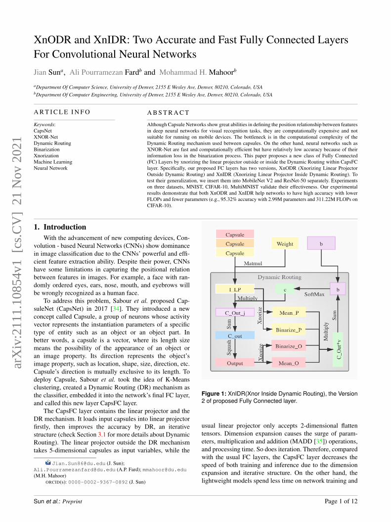
XnODR(Xnor Outside Dynamic Routing): ICap, ex-panded from IPrim, is different from standard tensors with

Sun et al.: Preprint Page 5 of 12

XnODR and XnIDR: Two Accurate and Fast Fully Connected Layers For Convolutional Neural Networks

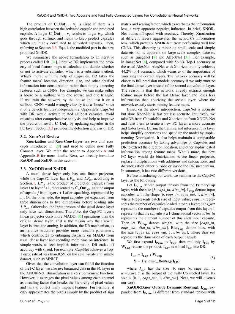
Figure 2: XnODR (Xnor Outside Dynamic Routing), theVersion 1 of proposed Fully Connected layer.

the shape [num_samples, flatten_features]. We will getan accurate binary filter if we xnorize ICap and its weightdirectly before the linear projector. However, we will alsoget an inaccurate scaling factor if we calculate averagevalue cross all dimensions, such that dimension 0, 1, and2 of WCap denote weight, with the shape of [caps_in,caps_out, dim_in, dim_out]. Moreover, the linear projectoris to change the size of the capsule vector from [1, dim_in]to [1, dim_out]. Inspired by this idea, we design a function,XLP, to address this problem by decomposing tensorsand Xnorize linear project the inner two dimensions, andformulate them in Eq.6:

Iin,Win = Scan(Scan(Scan(ICap),WCap))

Iin ∗ Win ≈ (BIin ⊛ BWin)⊙ �Iin �Win

IXLP[p,i, j, ∶, ∶] = Iin ∗ Win, p ∈ [0, b],i ∈ [0,caps_in], j ∈ [0, caps_out].

(6)

where Iin represents the inner two dimensions of ICapwith the shape [1, dim_in], Win represents the inner 2dimensions of WCap with the shape [dim_in, dim_out], BIindenotes the binary filter of Iin, ⊛ denotes the convolutionaloperation using XNOR and the bitcount operations, �Itheindenotes the scaling factor of Iin, BWin

denotes the binaryfilter of Win, �Win

denotes the scaling factor of Win,IXLP[p, i, j, ∶, ∶]’s size is [1, dim_out]. Moreover, Scanfunction is to unpack the tensors on dimension 0 repeatlyuntil the inner two dimensions, because we hope to changethe capsule vector from [1, dimin] to [1, dimout].

Next step, we put the XLP’s output, IXLP with the shape[b, caps_in, caps_out, 1, dim_out], into DR mechanism to

get final output, Y:

Y = Dynamic_Routing(IXLP). (7)

The detail of DR mechanism is introduced in Sec-tion.3.1. According to the [29], the total number of oper-ations in a standard convolution is cNWNI , where c ischannel number,NW = wℎ, NI = winℎin. With the currentgeneration of CPUs, we can perform 64 binary operations inone clock of CPU. The total parameters from the xnorizedconvolution is 1

64cNWNI + NI , where cNWNI is binaryoperations, NI is non-binary operations. The speed-ratioequation is summarized as Eq.8:

S =cNWNI

164cNWNI +NI

(8)

In our case, we only compare the operation times oflinear projector before DR, since we only binarize this partin XnODR. We take ICap, Capsules, as input for linearprojector, andNI as each capsule’s dimension. We also takeWCap as related weight, and NW as the product of diminand dimout. Therefore, we formulate the operations of theusual linear projector as Eq.9:

capsincapsout × dimoutdimindimout, (9)

the operations of binary one is formulated as Eq.10:

164capsincapsout × dimoutdimindimout + capsout. (10)

Therefore, the speed-ratio is :

capsincapsoutdim2outdimin

164capsincapsoutdim

2outdimin + dimin

. (11)

The result is shown in Section.4.XnIDR(Xnor Inside Dynamic Routing): There is Eq.1

within Dynamic Routing. We propose to use binarization asan insert function to simplify Eq.4, such that Eq.12:

bij = bij + C_Outj|i ⋅ vj (12)

where vj has the shape, [b, 1, caps_out, 1, dim_out],C_Outj|i has the shape, [b, caps_in, caps_out, 1, dim_out].

Given that the filter size is easily converted to 1×1, we donot need to do XnorConv here but think out a new way todo xnorized linear projector, which is doing average on thelast axis and dot product across all binary filters and scalingfilters. We formulate the above as Eq.13:

C_Outj|i ⋅ vj ≈ (B C_Outj|i⊙ Bvj )⊙ � C_Outj|i

�vjbij = bij + (B C_Outj|i

⊙ Bvj )⊙ � C_Outj|i�vj

(13)

B C_Outj|idenotes the binary filter of C_Outj|i, � C_Outj|i

denotes the scaling factor of C_Outj|i, Bvj denotes thebinary filter of vj, �vj denotes the scaling factor of vj.

Sun et al.: Preprint Page 6 of 12

XnODR and XnIDR: Two Accurate and Fast Fully Connected Layers For Convolutional Neural Networks

C_Outj|i ⋅ vj’s output shape is [b, caps_in, caps_out, 1,dim_out], then it gets summed across axis 1. Therefore, thefinal output shape is [b, 1, caps_out, 1, dim_out] matchingwith bij .

In the meanwhile, we only compare the operation timesof linear projector within DR for Speed Up, since we onlyxnorize this part in XnIDR. Here, we use C_Outj|i torepresent input for linear projector, which is a tensor ofcapsules, and select vj to represent weight for the linearprojector. Therefore, we formulate the operations of theusual linear projector as Eq.14:

caps_in × caps_out × dim_out2, (14)

the operations of binary one is formulated as Eq.15:

164caps_in × caps_out × dim_out2 + dim_out. (15)

The speedration ratio is formulated as Eq.16:

caps_in × caps_out × dim_out2164caps_in × caps_out × dim_out2 + dim_out

. (16)

The result is shown in Section.4.Summary: There are two linear projectors in the origi-

nal CapsFCLayer [34]. One is outside DR, while the otheris inside DR. XnODR xnorizes the linear projector outsideDR. XnIDR xnorizes the one inside DR. Therefore, XnODRand XnIDR simplify operations by xnorizing linear projec-tors at different positions. However, XnODR causes moreinformation loss than XnIDR, because XnIDR preservesall information in the outer linear projector. If the networkimplements Xnorization operation on both linear projectorssimultaneously, it lacks too much information to predictwell. In addition, to reduce the effect of the trade-offbetween speed and accuracy, we select Linear Transform(LT) and Group Linear Transform (GLT) to calculate linearprojector. LT and GLT help switch a broad and shallownetwork to a narrow and deep one and maintain the sameeffectiveness or even elevate it. In the meantime, the totalparameters get decreased. In general, LT and GLT canrelieve trading off between accuracy with speed.

4. ExperimentIn this section, we firstly introduce the datasets, evalua-

tion metrics, and implementation details. Then, we explainour experiments, present results, and analyze them.

4.1. DatasetsWe pick both small-scale datasets (MNIST [21], CIFAR-

10 [20]) and large-scale datasets (MultiMnist [34]) tovalidate our proposed XnODR and XnIDR. They wouldseparately work as the only FC layer in the MobileNet V2[35] (lightweight model) and the ResNet-50 [14] (heavy-weight model) to replace the original dense layers. Thesevariants are to validate XnODR’s and XnIDR’s effectivenesson those datasets.

MNIST: The National Institute of Standards and Tech-nology was in charge of creating the MNIST dataset [21].It consists of 70,000 28×28 gray-scale images in 10 classes.There are 60,000 training images and 10,000 test images.The American Census Bureau employees contributed tohalf of the training images, American high school studentscontributed the other half. So do test images. The categoriesare 0, 1, 2, 3, 4, 5, 6, 7, 8, and 9.

CIFAR-10: This dataset was collected by Alex Krizhevsky,Vinod Nair, and Geoffrey Hinton [20]. It consists of 60,00032×32 color images in 10 classes, with 6,000 images perclass. There are 50,000 training images and 10,000 testimages. The categories consist of airplane, automobile, bird,cat, deer, dog, frog, horse, ship, and truck.

MultiMNIST: This dataset is generated out of MNIST[21] to prove the effectiveness of CapsNet. Our proposedlayers are inspired by CapsNet, therefore, we also validatethe XnODR and XnIDR by MultiMNIST [34].

We create MultiMNIST2 following the instruction from[34], except generating 4 rather than 1K MultiMNIST [34]examples for each digit in the MNIST [21] dataset, becausewe find that the model can converge to accuracy higher than99% without a large volume dataset. So the training setconsists of 240,000 36×36 gray-scale images in 10 classes,and the test set size is 40,000 36×36 gray-scale images in10 classes. The categories are 0, 1, 2, 3, 4, 5, 6, 7, 8, and 9.

4.2. Evaluation MetricsThis paper takes prediction accuracy (the maximum

value among five random training), network parameters,Speed Up, and FLOPs as metrics to evaluate and comparethe model performance. Moreover, we would train Net-works like ResNet-50 [14], and MobileNet V2 [35] fromscratching again to record the metrics used in this paper butmissing in the original article.

4.3. Implementation DetailsWe first explain hyperparameters, experiment order,

packages’ versions, and GPU configuration used in thiswork.

For the MNIST [21] classification task, we take gray-scale images with the shape of [28, 28, 1] as the input valuesand convert labels to categorical values with the size of [b,10].

For the CIFAR-10 [20] classification task, we take colorimages with the shape of [32, 32, 3] as the input valuesand convert labels to categorical values with the size of[b, 10]. To enhance the performance, we do random dataaugmentation on CIFAR-10 [20] before training.

For the MultiMNIST [34] classification task, we takegray-scale images with the shape of [36, 36, 1] as the inputvalues and convert labels to categorical values with the sizeof [b, 10]. We do not do data augmentation on MultiMNIST[34].

2https://github.com/jiansfoggy/CODE-SHOW/blob/master/Python/Multi_Mnist/fast_generate_multimnist.py

Sun et al.: Preprint Page 7 of 12

XnODR and XnIDR: Two Accurate and Fast Fully Connected Layers For Convolutional Neural Networks

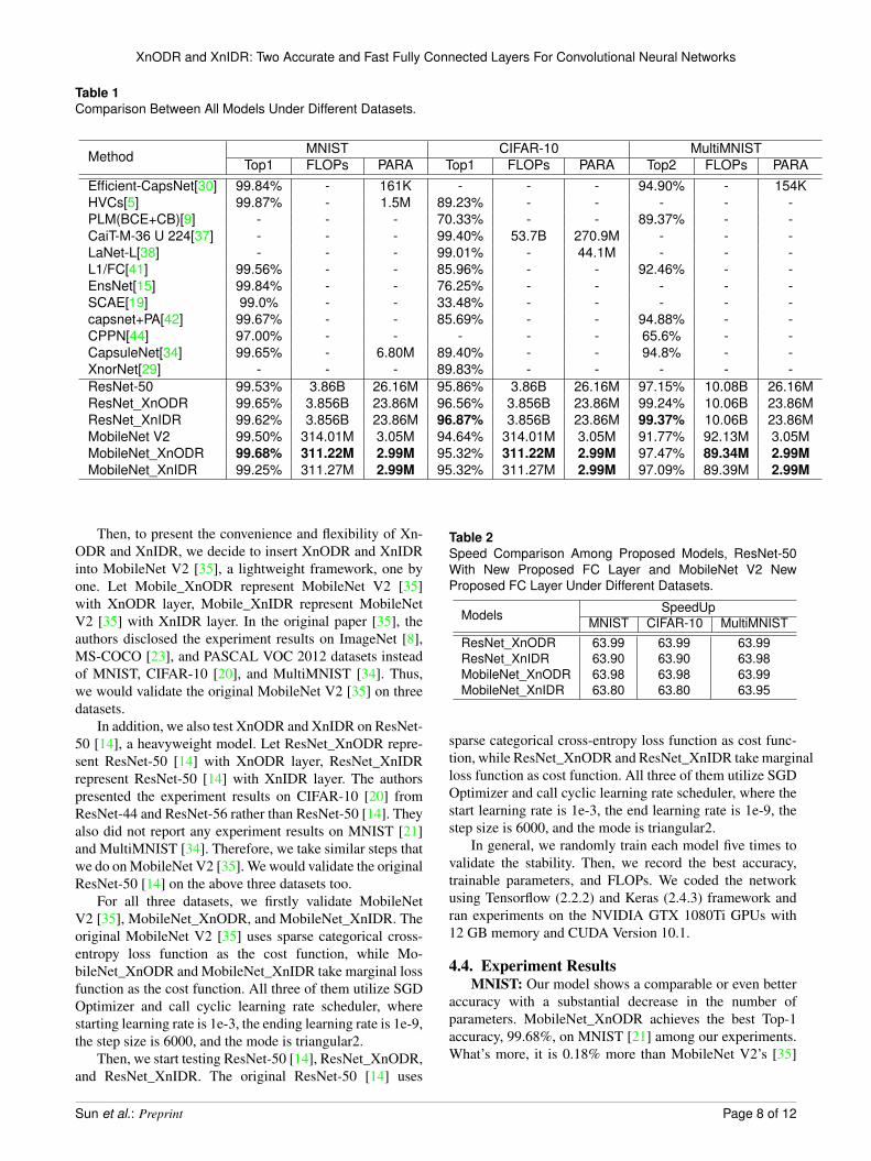
Table 1Comparison Between All Models Under Different Datasets.

Method MNIST CIFAR-10 MultiMNISTTop1 FLOPs PARA Top1 FLOPs PARA Top2 FLOPs PARA

Efficient-CapsNet[30] 99.84% - 161K - - - 94.90% - 154KHVCs[5] 99.87% - 1.5M 89.23% - - - - -PLM(BCE+CB)[9] - - - 70.33% - - 89.37% - -CaiT-M-36 U 224[37] - - - 99.40% 53.7B 270.9M - - -LaNet-L[38] - - - 99.01% - 44.1M - - -L1/FC[41] 99.56% - - 85.96% - - 92.46% - -EnsNet[15] 99.84% - - 76.25% - - - - -SCAE[19] 99.0% - - 33.48% - - - - -capsnet+PA[42] 99.67% - - 85.69% - - 94.88% - -CPPN[44] 97.00% - - - - - 65.6% - -CapsuleNet[34] 99.65% - 6.80M 89.40% - - 94.8% - -XnorNet[29] - - - 89.83% - - - - -ResNet-50 99.53% 3.86B 26.16M 95.86% 3.86B 26.16M 97.15% 10.08B 26.16MResNet_XnODR 99.65% 3.856B 23.86M 96.56% 3.856B 23.86M 99.24% 10.06B 23.86MResNet_XnIDR 99.62% 3.856B 23.86M 96.87% 3.856B 23.86M 99.37% 10.06B 23.86MMobileNet V2 99.50% 314.01M 3.05M 94.64% 314.01M 3.05M 91.77% 92.13M 3.05MMobileNet_XnODR 99.68% 311.22M 2.99M 95.32% 311.22M 2.99M 97.47% 89.34M 2.99MMobileNet_XnIDR 99.25% 311.27M 2.99M 95.32% 311.27M 2.99M 97.09% 89.39M 2.99M

Then, to present the convenience and flexibility of Xn-ODR and XnIDR, we decide to insert XnODR and XnIDRinto MobileNet V2 [35], a lightweight framework, one byone. Let Mobile_XnODR represent MobileNet V2 [35]with XnODR layer, Mobile_XnIDR represent MobileNetV2 [35] with XnIDR layer. In the original paper [35], theauthors disclosed the experiment results on ImageNet [8],MS-COCO [23], and PASCAL VOC 2012 datasets insteadof MNIST, CIFAR-10 [20], and MultiMNIST [34]. Thus,we would validate the original MobileNet V2 [35] on threedatasets.

In addition, we also test XnODR and XnIDR on ResNet-50 [14], a heavyweight model. Let ResNet_XnODR repre-sent ResNet-50 [14] with XnODR layer, ResNet_XnIDRrepresent ResNet-50 [14] with XnIDR layer. The authorspresented the experiment results on CIFAR-10 [20] fromResNet-44 and ResNet-56 rather than ResNet-50 [14]. Theyalso did not report any experiment results on MNIST [21]and MultiMNIST [34]. Therefore, we take similar steps thatwe do on MobileNet V2 [35]. We would validate the originalResNet-50 [14] on the above three datasets too.

For all three datasets, we firstly validate MobileNetV2 [35], MobileNet_XnODR, and MobileNet_XnIDR. Theoriginal MobileNet V2 [35] uses sparse categorical cross-entropy loss function as the cost function, while Mo-bileNet_XnODR and MobileNet_XnIDR take marginal lossfunction as the cost function. All three of them utilize SGDOptimizer and call cyclic learning rate scheduler, wherestarting learning rate is 1e-3, the ending learning rate is 1e-9,the step size is 6000, and the mode is triangular2.

Then, we start testing ResNet-50 [14], ResNet_XnODR,and ResNet_XnIDR. The original ResNet-50 [14] uses

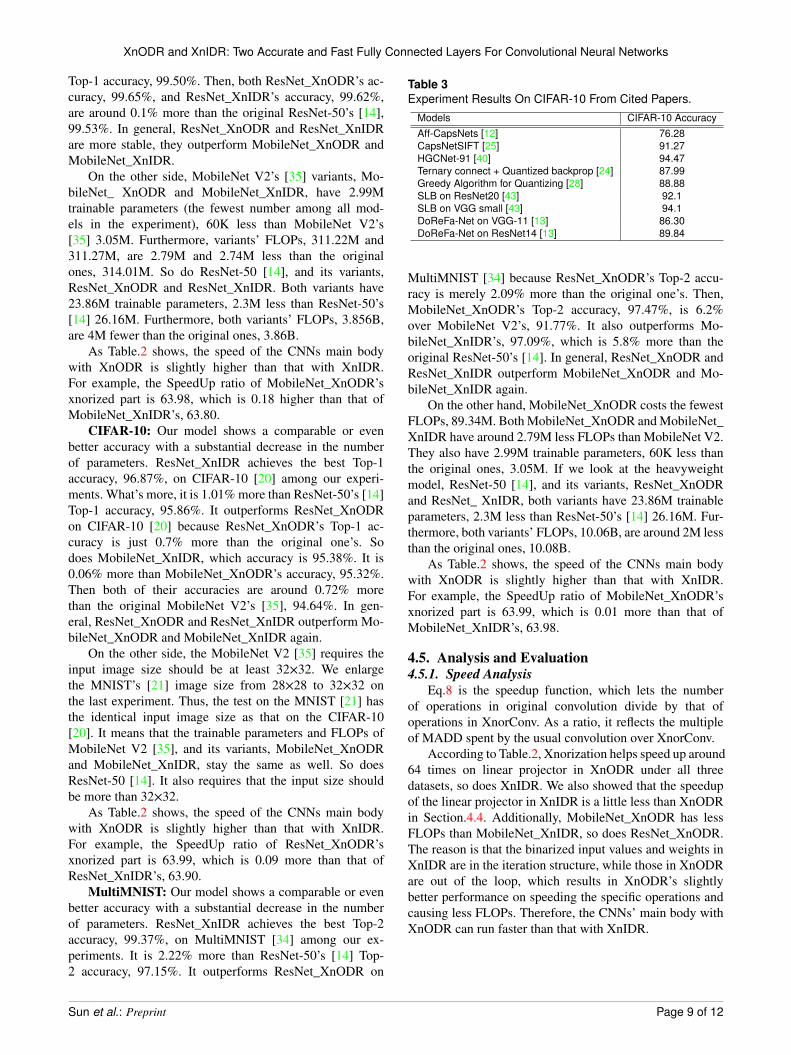
Table 2Speed Comparison Among Proposed Models, ResNet-50With New Proposed FC Layer and MobileNet V2 NewProposed FC Layer Under Different Datasets.

Models SpeedUpMNIST CIFAR-10 MultiMNIST

ResNet_XnODR 63.99 63.99 63.99ResNet_XnIDR 63.90 63.90 63.98MobileNet_XnODR 63.98 63.98 63.99MobileNet_XnIDR 63.80 63.80 63.95

sparse categorical cross-entropy loss function as cost func-tion, while ResNet_XnODR and ResNet_XnIDR take marginalloss function as cost function. All three of them utilize SGDOptimizer and call cyclic learning rate scheduler, where thestart learning rate is 1e-3, the end learning rate is 1e-9, thestep size is 6000, and the mode is triangular2.

In general, we randomly train each model five times tovalidate the stability. Then, we record the best accuracy,trainable parameters, and FLOPs. We coded the networkusing Tensorflow (2.2.2) and Keras (2.4.3) framework andran experiments on the NVIDIA GTX 1080Ti GPUs with12 GB memory and CUDA Version 10.1.

4.4. Experiment ResultsMNIST: Our model shows a comparable or even better

accuracy with a substantial decrease in the number ofparameters. MobileNet_XnODR achieves the best Top-1accuracy, 99.68%, on MNIST [21] among our experiments.What’s more, it is 0.18% more than MobileNet V2’s [35]

Sun et al.: Preprint Page 8 of 12

XnODR and XnIDR: Two Accurate and Fast Fully Connected Layers For Convolutional Neural Networks

Top-1 accuracy, 99.50%. Then, both ResNet_XnODR’s ac-curacy, 99.65%, and ResNet_XnIDR’s accuracy, 99.62%,are around 0.1% more than the original ResNet-50’s [14],99.53%. In general, ResNet_XnODR and ResNet_XnIDRare more stable, they outperform MobileNet_XnODR andMobileNet_XnIDR.

On the other side, MobileNet V2’s [35] variants, Mo-bileNet_ XnODR and MobileNet_XnIDR, have 2.99Mtrainable parameters (the fewest number among all mod-els in the experiment), 60K less than MobileNet V2’s[35] 3.05M. Furthermore, variants’ FLOPs, 311.22M and311.27M, are 2.79M and 2.74M less than the originalones, 314.01M. So do ResNet-50 [14], and its variants,ResNet_XnODR and ResNet_XnIDR. Both variants have23.86M trainable parameters, 2.3M less than ResNet-50’s[14] 26.16M. Furthermore, both variants’ FLOPs, 3.856B,are 4M fewer than the original ones, 3.86B.

As Table.2 shows, the speed of the CNNs main bodywith XnODR is slightly higher than that with XnIDR.For example, the SpeedUp ratio of MobileNet_XnODR’sxnorized part is 63.98, which is 0.18 higher than that ofMobileNet_XnIDR’s, 63.80.

CIFAR-10: Our model shows a comparable or evenbetter accuracy with a substantial decrease in the numberof parameters. ResNet_XnIDR achieves the best Top-1accuracy, 96.87%, on CIFAR-10 [20] among our experi-ments. What’s more, it is 1.01% more than ResNet-50’s [14]Top-1 accuracy, 95.86%. It outperforms ResNet_XnODRon CIFAR-10 [20] because ResNet_XnODR’s Top-1 ac-curacy is just 0.7% more than the original one’s. Sodoes MobileNet_XnIDR, which accuracy is 95.38%. It is0.06% more than MobileNet_XnODR’s accuracy, 95.32%.Then both of their accuracies are around 0.72% morethan the original MobileNet V2’s [35], 94.64%. In gen-eral, ResNet_XnODR and ResNet_XnIDR outperform Mo-bileNet_XnODR and MobileNet_XnIDR again.

On the other side, the MobileNet V2 [35] requires theinput image size should be at least 32×32. We enlargethe MNIST’s [21] image size from 28×28 to 32×32 onthe last experiment. Thus, the test on the MNIST [21] hasthe identical input image size as that on the CIFAR-10[20]. It means that the trainable parameters and FLOPs ofMobileNet V2 [35], and its variants, MobileNet_XnODRand MobileNet_XnIDR, stay the same as well. So doesResNet-50 [14]. It also requires that the input size shouldbe more than 32×32.

As Table.2 shows, the speed of the CNNs main bodywith XnODR is slightly higher than that with XnIDR.For example, the SpeedUp ratio of ResNet_XnODR’sxnorized part is 63.99, which is 0.09 more than that ofResNet_XnIDR’s, 63.90.

MultiMNIST: Our model shows a comparable or evenbetter accuracy with a substantial decrease in the numberof parameters. ResNet_XnIDR achieves the best Top-2accuracy, 99.37%, on MultiMNIST [34] among our ex-periments. It is 2.22% more than ResNet-50’s [14] Top-2 accuracy, 97.15%. It outperforms ResNet_XnODR on

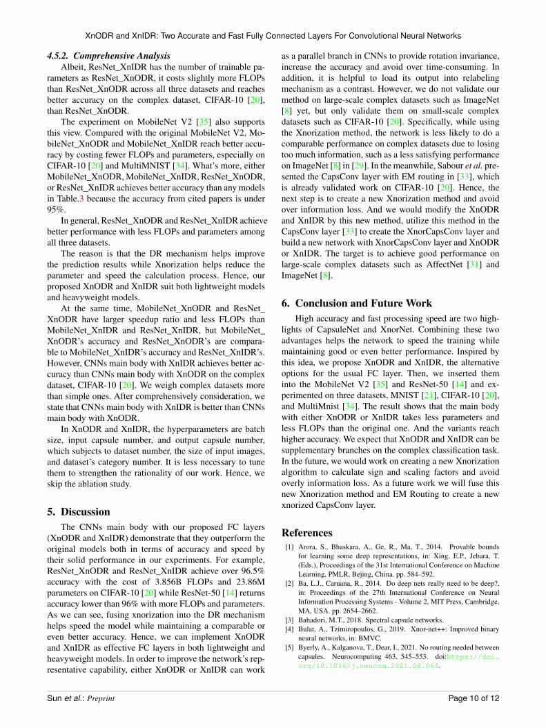
Table 3Experiment Results On CIFAR-10 From Cited Papers.

Models CIFAR-10 AccuracyAff-CapsNets [12] 76.28CapsNetSIFT [25] 91.27HGCNet-91 [40] 94.47Ternary connect + Quantized backprop [24] 87.99Greedy Algorithm for Quantizing [28] 88.88SLB on ResNet20 [43] 92.1SLB on VGG small [43] 94.1DoReFa-Net on VGG-11 [13] 86.30DoReFa-Net on ResNet14 [13] 89.84

MultiMNIST [34] because ResNet_XnODR’s Top-2 accu-racy is merely 2.09% more than the original one’s. Then,MobileNet_XnODR’s Top-2 accuracy, 97.47%, is 6.2%over MobileNet V2’s, 91.77%. It also outperforms Mo-bileNet_XnIDR’s, 97.09%, which is 5.8% more than theoriginal ResNet-50’s [14]. In general, ResNet_XnODR andResNet_XnIDR outperform MobileNet_XnODR and Mo-bileNet_XnIDR again.

On the other hand, MobileNet_XnODR costs the fewestFLOPs, 89.34M. Both MobileNet_XnODR and MobileNet_XnIDR have around 2.79M less FLOPs than MobileNet V2.They also have 2.99M trainable parameters, 60K less thanthe original ones, 3.05M. If we look at the heavyweightmodel, ResNet-50 [14], and its variants, ResNet_XnODRand ResNet_ XnIDR, both variants have 23.86M trainableparameters, 2.3M less than ResNet-50’s [14] 26.16M. Fur-thermore, both variants’ FLOPs, 10.06B, are around 2M lessthan the original ones, 10.08B.

As Table.2 shows, the speed of the CNNs main bodywith XnODR is slightly higher than that with XnIDR.For example, the SpeedUp ratio of MobileNet_XnODR’sxnorized part is 63.99, which is 0.01 more than that ofMobileNet_XnIDR’s, 63.98.

4.5. Analysis and Evaluation4.5.1. Speed Analysis

Eq.8 is the speedup function, which lets the numberof operations in original convolution divide by that ofoperations in XnorConv. As a ratio, it reflects the multipleof MADD spent by the usual convolution over XnorConv.

According to Table.2, Xnorization helps speed up around64 times on linear projector in XnODR under all threedatasets, so does XnIDR. We also showed that the speedupof the linear projector in XnIDR is a little less than XnODRin Section.4.4. Additionally, MobileNet_XnODR has lessFLOPs than MobileNet_XnIDR, so does ResNet_XnODR.The reason is that the binarized input values and weights inXnIDR are in the iteration structure, while those in XnODRare out of the loop, which results in XnODR’s slightlybetter performance on speeding the specific operations andcausing less FLOPs. Therefore, the CNNs’ main body withXnODR can run faster than that with XnIDR.

Sun et al.: Preprint Page 9 of 12

XnODR and XnIDR: Two Accurate and Fast Fully Connected Layers For Convolutional Neural Networks

4.5.2. Comprehensive AnalysisAlbeit, ResNet_XnIDR has the number of trainable pa-

rameters as ResNet_XnODR, it costs slightly more FLOPsthan ResNet_XnODR across all three datasets and reachesbetter accuracy on the complex dataset, CIFAR-10 [20],than ResNet_XnODR.

The experiment on MobileNet V2 [35] also supportsthis view. Compared with the original MobileNet V2, Mo-bileNet_XnODR and MobileNet_XnIDR reach better accu-racy by costing fewer FLOPs and parameters, especially onCIFAR-10 [20] and MultiMNIST [34]. What’s more, eitherMobileNet_XnODR, MobileNet_XnIDR, ResNet_XnODR,or ResNet_XnIDR achieves better accuracy than any modelsin Table.3 because the accuracy from cited papers is under95%.

In general, ResNet_XnODR and ResNet_XnIDR achievebetter performance with less FLOPs and parameters amongall three datasets.

The reason is that the DR mechanism helps improvethe prediction results while Xnorization helps reduce theparameter and speed the calculation process. Hence, ourproposed XnODR and XnIDR suit both lightweight modelsand heavyweight models.

At the same time, MobileNet_XnODR and ResNet_XnODR have larger speedup ratio and less FLOPs thanMobileNet_XnIDR and ResNet_XnIDR, but MobileNet_XnODR’s accuracy and ResNet_XnODR’s are compara-ble to MobileNet_XnIDR’s accuracy and ResNet_XnIDR’s.However, CNNs main body with XnIDR achieves better ac-curacy than CNNs main body with XnODR on the complexdataset, CIFAR-10 [20]. We weigh complex datasets morethan simple ones. After comprehensively consideration, westate that CNNs main body with XnIDR is better than CNNsmain body with XnODR.

In XnODR and XnIDR, the hyperparameters are batchsize, input capsule number, and output capsule number,which subjects to dataset number, the size of input images,and dataset’s category number. It is less necessary to tunethem to strengthen the rationality of our work. Hence, weskip the ablation study.

5. DiscussionThe CNNs main body with our proposed FC layers

(XnODR and XnIDR) demonstrate that they outperform theoriginal models both in terms of accuracy and speed bytheir solid performance in our experiments. For example,ResNet_XnODR and ResNet_XnIDR achieve over 96.5%accuracy with the cost of 3.856B FLOPs and 23.86Mparameters on CIFAR-10 [20] while ResNet-50 [14] returnsaccuracy lower than 96% with more FLOPs and parameters.As we can see, fusing xnorization into the DR mechanismhelps speed the model while maintaining a comparable oreven better accuracy. Hence, we can implement XnODRand XnIDR as effective FC layers in both lightweight andheavyweight models. In order to improve the network’s rep-resentative capability, either XnODR or XnIDR can work

as a parallel branch in CNNs to provide rotation invariance,increase the accuracy and avoid over time-consuming. Inaddition, it is helpful to load its output into relabelingmechanism as a contrast. However, we do not validate ourmethod on large-scale complex datasets such as ImageNet[8] yet, but only validate them on small-scale complexdatasets such as CIFAR-10 [20]. Specifically, while usingthe Xnorization method, the network is less likely to do acomparable performance on complex datasets due to losingtoo much information, such as a less satisfying performanceon ImageNet [8] in [29]. In the meanwhile, Sabour et al. pre-sented the CapsConv layer with EM routing in [33], whichis already validated work on CIFAR-10 [20]. Hence, thenext step is to create a new Xnorization method and avoidover information loss. And we would modify the XnODRand XnIDR by this new method, utilize this method in theCapsConv layer [33] to create the XnorCapsConv layer andbuild a new network with XnorCapsConv layer and XnODRor XnIDR. The target is to achieve good performance onlarge-scale complex datasets such as AffectNet [31] andImageNet [8].

6. Conclusion and Future WorkHigh accuracy and fast processing speed are two high-

lights of CapsuleNet and XnorNet. Combining these twoadvantages helps the network to speed the training whilemaintaining good or even better performance. Inspired bythis idea, we propose XnODR and XnIDR, the alternativeoptions for the usual FC layer. Then, we inserted theminto the MobileNet V2 [35] and ResNet-50 [14] and ex-perimented on three datasets, MNIST [21], CIFAR-10 [20],and MultiMnist [34]. The result shows that the main bodywith either XnODR or XnIDR takes less parameters andless FLOPs than the original one. And the variants reachhigher accuracy. We expect that XnODR and XnIDR can besupplementary branches on the complex classification task.In the future, we would work on creating a new Xnorizationalgorithm to calculate sign and scaling factors and avoidoverly information loss. As a future work we will fuse thisnew Xnorization method and EM Routing to create a newxnorized CapsConv layer.

References[1] Arora, S., Bhaskara, A., Ge, R., Ma, T., 2014. Provable bounds

for learning some deep representations, in: Xing, E.P., Jebara, T.(Eds.), Proceedings of the 31st International Conference on MachineLearning, PMLR, Bejing, China. pp. 584–592.

[2] Ba, L.J., Caruana, R., 2014. Do deep nets really need to be deep?,in: Proceedings of the 27th International Conference on NeuralInformation Processing Systems - Volume 2, MIT Press, Cambridge,MA, USA. pp. 2654–2662.

[3] Bahadori, M.T., 2018. Spectral capsule networks.[4] Bulat, A., Tzimiropoulos, G., 2019. Xnor-net++: Improved binary

neural networks, in: BMVC.[5] Byerly, A., Kalganova, T., Dear, I., 2021. No routing needed between

capsules. Neurocomputing 463, 545–553. doi:https://doi.org/10.1016/j.neucom.2021.08.064.

Sun et al.: Preprint Page 10 of 12

XnODR and XnIDR: Two Accurate and Fast Fully Connected Layers For Convolutional Neural Networks

[6] Cybenko, G., 1989. Approximation by superpositions of a sig-moidal function. Mathematics of Control, Signals, and Systems(MCSS) 2, 303–314. URL: http://dx.doi.org/10.1007/BF02551274, doi:10.1007/BF02551274.

[7] Dauphin, Y., Bengio, Y., 2013. Big neural networks waste capacity.CoRR abs/1301.3583.

[8] Deng, J., Dong, W., Socher, R., Li, L.J., Li, K., Fei-Fei, L., 2009.Imagenet: A large-scale hierarchical image database, in: 2009 IEEEConference on Computer Vision and Pattern Recognition, pp. 248–255. doi:10.1109/CVPR.2009.5206848.

[9] Duarte, K., Rawat, Y., Shah, M., 2021. Plm: Partial label maskingfor imbalanced multi-label classification, in: Proceedings of theIEEE/CVF Conference on Computer Vision and Pattern Recognition(CVPR) Workshops, pp. 2739–2748.

[10] Floropoulos, N., Tefas, A., 2019. Complete vector quantiza-tion of feedforward neural networks. Neurocomputing 367,55–63. doi:https://doi.org/10.1016/j.neucom.2019.08.003.

[11] Gong, Y., Liu, L., Yang, M., Bourdev, L., 2014. Compressing DeepConvolutional Networks using Vector Quantization. arXiv e-prints ,arXiv:1412.6115arXiv:1412.6115.

[12] Gu, J., Tresp, V., 2020. Improving the robustness of capsule networksto image affine transformations. 2020 IEEE/CVF Conference onComputer Vision and Pattern Recognition (CVPR) , 7283–7291.

[13] Guerra, L., Zhuang, B., Reid, I., Drummond, T., 2020. Auto-matic Pruning for Quantized Neural Networks. arXiv e-prints ,arXiv:2002.00523arXiv:2002.00523.

[14] He, K., Zhang, X., Ren, S., Sun, J., 2016. Deep residual learning forimage recognition. 2016 IEEE Conference on Computer Vision andPattern Recognition (CVPR) , 770–778.

[15] Hirata, D., Takahashi, N., 2020. Ensemble learning in CNNaugmented with fully connected subnetworks. arXiv e-prints ,arXiv:2003.08562arXiv:2003.08562.

[16] Hwang, K., Sung, W., 2014. Fixed-point feedforward deep neuralnetwork design using weights +1, 0, and -1, in: 2014 IEEE Workshopon Signal Processing Systems (SiPS), pp. 1–6. doi:10.1109/SiPS.2014.6986082.

[17] Iandola, F.N., Han, S., Moskewicz, M.W., Ashraf, K., Dally, W.J.,Keutzer, K., 2016. SqueezeNet: AlexNet-level accuracy with50x fewer parameters and <0.5MB model size. arXiv e-prints ,arXiv:1602.07360arXiv:1602.07360.

[18] Kim, J., Jang, S., Park, E., Choi, S., 2020. Text classification usingcapsules. Neurocomputing 376, 214–221.

[19] Kosiorek, A.R., Sabour, S., Teh, Y.W., Hinton, G., 2019. Stackedcapsule autoencoders, in: Neural Information Processing Systems.URL: https://arxiv.org/pdf/1906.06818.pdf.

[20] Krizhevsky, A., Nair, V., Hinton, G., . Cifar-10 (canadian institutefor advanced research) URL: http://www.cs.toronto.edu/~kriz/cifar.html.

[21] LeCun, Y., Cortes, C., 2010. MNIST handwritten digit databaseURL: http://yann.lecun.com/exdb/mnist/.

[22] Lenssen, J.E., Fey, M., Libuschewski, P., 2018. Group equivariantcapsule networks, in: NeurIPS, pp. 8858–8867.

[23] Lin, T.Y., Maire, M., Belongie, S., Hays, J., Perona, P., Ramanan, D.,Dollár, P., Zitnick, C.L., 2014. Microsoft coco: Common objects incontext, in: Fleet, D., Pajdla, T., Schiele, B., Tuytelaars, T. (Eds.),Computer Vision – ECCV 2014, Springer International Publishing,Cham. pp. 740–755.

[24] Lin, Z., Courbariaux, M., Memisevic, R., Bengio, Y., 2016. Neuralnetworks with few multiplications, in: Bengio, Y., LeCun, Y. (Eds.),4th International Conference on Learning Representations, ICLR2016, San Juan, Puerto Rico, May 2-4, 2016, Conference TrackProceedings. URL: http://arxiv.org/abs/1510.03009.

[25] Lin, Z., Gao, W., Jia, J., Huang, F., 2021a. Capsnet meets sift: A ro-bust framework for distorted target categorization. Neurocomputing464, 290–316. doi:https://doi.org/10.1016/j.neucom.2021.08.087.

[26] Lin, Z., Jia, J., Huang, F., Gao, W., 2021b. A coarse-to-fine capsulenetwork for fine-grained image categorization. Neurocomputing456, 200–219. doi:https://doi.org/10.1016/j.neucom.2021.05.032.

[27] Liu, Z., Luo, W., Wu, B., Yang, X., Liu, W., Cheng, K., 2019. Bi-real net: Binarizing deep network towards real-network performance.International Journal of Computer Vision 128, 202–219.

[28] Lybrand, E., Saab, R., 2020. A Greedy Algorithm for Quantiz-ing Neural Networks. Journal of Machine Learning Research ,arXiv:2010.15979arXiv:2010.15979.

[29] M. Rastegari, V. Ordonez, J.R., Farhadi, A., 2016. Xnor-net:Imagenet classification using binary convolutional neural networks,in: European Conference on Computer Vision (ECCV), Springer. pp.525–542.

[30] Mazzia, V., Salvetti, F., Chiaberge, M., 2021. Efficient-capsnet:Capsule network with self-attention routing. Scientific Reports 11.

[31] Mollahosseini, A., Hasani, B., Mahoor, M.H., 2019. Affectnet: Adatabase for facial expression, valence, and arousal computing in thewild. IEEE Transactions on Affective Computing 10, 18–31.

[32] Ribeiro, F., Leontidis, G., Kollias, S., 2019. Capsulerouting via variational bayes, pp. 1–8. URL: https://aaai.org/Conferences/AAAI-20/, doi:10.1609/aaai.v34i04.5785. 34th AAAI 2020 Accepted Paper -Flagship/Top conference with very high h-index; Thirty-FourthAAAI Conference on Artificial Intelligence, AAAI ; Conferencedate: 07-02-2020 Through 12-02-2020.

[33] S. Sabour, G.E.H., Frosst, N., 2018. Matrix capsules with em routing,in: International Conference on Learning Representations (ICLR).

[34] S. Sabour, N.F., Hinton, G.E., 2017. Dynamic routing betweencapsules., in: Neural Information Processing Systems (NIPS).

[35] Sandler, M., Howard, A.G., Zhu, M., Zhmoginov, A., Chen, L.C.,2018. Mobilenetv2: Inverted residuals and linear bottlenecks. 2018IEEE/CVF Conference on Computer Vision and Pattern Recognition, 4510–4520.

[36] Szegedy, C., Liu, W., Jia, Y., Sermanet, P., Reed, S., Anguelov, D.,Erhan, D., Vanhoucke, V., Rabinovich, A., 2015. Going deeperwith convolutions, in: 2015 IEEE Conference on Computer Visionand Pattern Recognition (CVPR), pp. 1–9. doi:10.1109/CVPR.2015.7298594.

[37] Touvron, H., Cord, M., Sablayrolles, A., Synnaeve, G., Jégou, H.,2021. Going deeper with Image Transformers. arXiv e-prints ,arXiv:2103.17239arXiv:2103.17239.

[38] Wang, L., Xie, S., Li, T., Fonseca, R., Tian, Y., 2019. Sample-Efficient Neural Architecture Search by Learning Action Space.arXiv e-prints , arXiv:1906.06832arXiv:1906.06832.

[39] Xi, E., Bing, S., Jin, Y., 2017. Capsule NetworkPerformance on Complex Data. arXiv e-prints ,arXiv:1712.03480arXiv:1712.03480.

[40] Xie, X., Zhou, Y., Kung, S.Y., 2020. Exploring highly efficientcompact neural networks for image classification, in: 2020 IEEEInternational Conference on Image Processing (ICIP), pp. 2930–2934. doi:10.1109/ICIP40778.2020.9191334.

[41] Yang, H., Li, S., Yu, B., 2021. Routing TowardsDiscriminative Power of Class Capsules. arXiv e-prints ,arXiv:2103.04278arXiv:2103.04278.

[42] Yang, Z., Wang, X., 2019. Reducing the dilution: Ananalysis of the information sensitiveness of capsule networkwith a practical improvement method. arXiv e-prints ,arXiv:1903.10588arXiv:1903.10588.

[43] Yang, Z., Wang, Y., Han, K., Xu, C., Xu, C., Tao, D., Xu, C., 2020.Searching for Low-Bit Weights in Quantized Neural Networks. arXive-prints , arXiv:2009.08695arXiv:2009.08695.

[44] Yao, H., Regan, M., Yang, Y., Ren, Y., 2019. Image decom-position and classification through a generative model, in: 2019IEEE International Conference on Image Processing, ICIP 2019 -Proceedings, IEEE Computer Society. pp. 400–404. doi:10.1109/ICIP.2019.8802991. publisher Copyright: © 2019 IEEE.; 26thIEEE International Conference on Image Processing, ICIP 2019 ;

Sun et al.: Preprint Page 11 of 12

XnODR and XnIDR: Two Accurate and Fast Fully Connected Layers For Convolutional Neural Networks

Conference date: 22-09-2019 Through 25-09-2019.[45] Yoshida, Y., Oiwa, R., Kawahara, T., 2018. Ternary sparse xnor-

net for fpga implementation, in: 2018 7th International Symposiumon Next Generation Electronics (ISNE), pp. 1–2. doi:10.1109/ISNE.2018.8394728.

[46] Yu, D., Seide, F., Li, G., 2012. Conversational speech transcriptionusing context-dependent deep neural networks, in: Proceedings ofthe 29th International Coference on International Conference onMachine Learning, Omnipress, Madison, WI, USA. pp. 1–2.

[47] Zhu, S., Duong, L.H.K., Liu, W., 2020. Xor-net: An efficientcomputation pipeline for binary neural network inference on edgedevices, in: 2020 IEEE 26th International Conference on Paralleland Distributed Systems (ICPADS), pp. 124–131. doi:10.1109/ICPADS51040.2020.00026.

A. XnorizationXnorization is to split the tensor into 2 parts. One is sign,

the other one is scaling factor.Let be a set of tensors. And I = l(l=1,...,L), I ∈

ℝc×win×ℎin represents the input tensor for the ltℎ layerof network, where (c, win, ℎin) means channel, width andheight. We split the tensor I into two values, binary filterB ∈ {+1,−1}c×win×ℎin and scaling factor � ∈ ℝ+, and usethem to estimate I ≈ �B.

We first discuss the Sign and the binary filter. According

to [29] k-bit Quantization is qk(x) = 2([(2k−1)( x+12 )]

2k−1 − 12 ).

The sign function is 1-bit Quantization, such that q1(x) =

2([(21−1)( x+12 )]

21−1 − 12 ) = 2(x+12 − 1

2 ), where the inner function,x+12 , is Hard Sigmoid function, the outer function, 2(Y −

12 ), is Tanh function. Therefore, the sign function can beformulated as shown in the Eq.17

BHS = Hard_Sigmoid(Round(INorm))

=Round(INorm) + 1

2(17)

where BHS is the output of Hard Sigmoid, INorm is theMin-Max Normalization result of I. Its range is [0,1]. Roundfunction will round value bigger than 0.5 to be 1, less than orequal to 0.5 to be 0. And it leaves INorm only 2 values, 0 and1 after rounding, then the output of Hard Sigmoid functionBHS ∈ {0.5, 1}. To control the value of BHS between 0 and1, we call Clip function and round its output, such that

BC = Clip(BHS) = max(0, min(1,BHS))BR = Round(BC).

(18)

Therefore, we get BR, which only has 2 values, 0 and 1.To get the expected binary filter B, we load BR into Tanhfunction, B = T anℎ(BR) = 2 × BC − 1 ∈ {−1,+1}. Now,we calculate the sign of I out.

About scaling factor, according to [29], we use theaverage of I to represent it.

� = 1n(ITB) =

∑

|Ii|n

= 1n||I||L1

(L1 −Norm) (19)

Eq.19 is the formula to get scaling factor, where �represents the scaling factor. Xnorization is the core ofXnorConvLayer, which is reviewed below.

B. XnorConvLayerXnorConvLayer is similar to the standard Conv layer,

except xnorizing input and weight before doing convolution.Therefore, XnorConvLayer has xnorized input values andxnorized weights. We formulate it as the following.

Let Ij denote jtℎ tensor of I, �Ij denote jtℎ scalingfactor, BI denote binary filter of I. Then I ≈ AIBI is theestimate of I after xnorize, where AI = {�I0 , �I1 , ..., �Iℎin }.

Then, let be a set of tensors, and W represent thektℎ weight filter in the ltℎ layer of the network such thatW = lk(k=1,...,K l). K l is the number of weight filters in theltℎ layer of the network. What’s more, W ∈ ℝc×w×ℎ, wherew ≤ win, ℎ ≤ ℎin.

Next, we start estimating W with binary filter, BW, andscaling filter, AW, such that W ≈ AWBW.

AW = {�W0, �W1

, ..., �Wj, ..., �Wℎin

}, where �Wjdenote

jtℎ scaling factor.According to XNOR-Net [29], Xnorization replaces

multiplication in convolutional operations with additionsand subtractions. And it causes 58× faster convolutionaloperations and 32× memory savings. This process is calledBinary Dot Product.

To approximate the dot product between X1 and X2,such that X1

TX2 ≈ �1B1T �2B2, where B1,B2 ∈ {+1,−1}n,

�1, �2 ∈ ℝ+, the paper solved and proved the followingoptimization:

�∗1 ,B∗1, �

∗2 ,B

∗2 = argmin

�1,B1,�2,B2

||X1⊙X2−�1�2B1⊙B2|| (20)

where ⊙ represents element-wise product.In the meanwhile, for input tensors, I, and weight, W,

we need to compute scaling factor, �Ij , for all possible sub-tensors in I with same size as W during convolution. Toovercome the redundant computations caused by overlapsbetween sub-tensors, the paper firstly computed a matrix

MI =∑

|I∶,∶,i|c , which is the average over absolute values

of the elements in the input I across the channel, c. Then thepaper convolved MI with a 2D filter k ∈ ℝw×ℎ, AI = MI ∗k, where ∀ij kij =

1w×ℎ and ∗ is a convolutional operation.

AI contains scaling factors �Ij for all sub-tensors in the inputI.

The above description proves that it makes sense toestimate I ∗ W by (BI ⊛ BW) ⊙ AI�W, which can beformulated as Eq.21:

I ∗ W ≈ (BI ⊛ BW)⊙ AI�W (21)

where ⊛ denotes the convolutional operation usingXNOR and the bitcount operations.

Sun et al.: Preprint Page 12 of 12