Embed Size (px)
Citation preview
Department of Construction Sciences
Solid Mechanics
ISRN LUTFD2/TFHF-14/5186-SE(1-84)
XFEM - Analysis and Implementation
Master’s Dissertation by
Simon Arnesson
Supervisors:Matti Ristinmaa, Division of Solid Mechanics
Examiner:Mathias Wallin , Division of Solid Mechanics
Copyright c© 2014 by the Division of Solid Mechanicsand Simon Arnesson
Printed by Media-Tryck AB, Lund, SwedenFor information, adress:
Division of Solid Mechanics, Lund University, Box 118, SE-221 00 Lund, SwedenWebpage: www.solid.lth.se

Abstract
The finite element method is a popular numerical approach for solving solid me-chanical and other types of engineering problems. This work addresses a developmentof the finite element method called the eXtended Finite Element Method, or XFEMfor short. This method is designed in order to simulate problems where some kindof discontinuity is present in the system’s governing equations. Something that isnot possible in the standard FE-method. This paper intends to outline the method’stheoretical foundation, discuss the merits of the method for solving a selection oftypical cases as well as evaluate a MATLAB implementation of the method that waswritten in conjunction with this work. Discussion points for the theoretical overvieware how one or several discontinuities’ geometrical properties can be efficiently storedand evaluated for different kinds of problems with the aid of a level set function, howa discontinuity’s physical behavior can be described by a enrichment function andhow the connection between the level set and enrichment functions and the standardFE-method works. The MATLAB program is evaluated in a series of test cases eachposing a specific challenge in adapting the XFEM approach to that kind of problem.
Sammanfattning
Finita element metoden ar ett populart verktyg for numerisk simulering av hallfasthets-och andra ingenjorsproblem. Detta verk behandlar en utveckling av finita element me-toden kallad eXtended Finite Element Method eller forkortat ”XFEM”’. Denna metodar utvecklad i syfte att kunna simulera fall dar nagon form av diskontinuitet finns ide ekvationer som styr det fysikaliska beteende som onskas beskrivas, nagot som intear mojligt i den vanliga finita element metoden. Denna studie ar gjord med avsiktatt ge en overgripande bild av XFE-metodens bakomliggande teori, diskutera moj-liga applikationsomraden samt att implementera metoden i ett MATLAB-programoch visa upp detta programs funktionalitet. Har avhandlas ett satt att beskriva endiskontinuitets geometri i form av en level set - funktion samt hur denna funktion an-passas till olika problem. Likasa skildras hur diskontinuiteters fysikaliska uppforandehanteras i metoden via vad som kallas berikningsfunktion samt hur denna kopplas tillstandard versionen av finita element metoden. Konkreta exempel dar berikningsfunk-tionen implementeras till olika typer av diskontinuiteter ges. MATLAB- programmetutvarderades i en serie exempelfall dar varje exempel skildrar anpassning av en ellerflera diskontinuiteters geometri och/eller fysikaliskt uppforande for en specifik typ avproblem.
1
Contents
1 Introduction 81.1 Purpose . . . . . . . . . . . . . . . . . . . . . . . . . . . . . . . . . . . . . 81.2 Background . . . . . . . . . . . . . . . . . . . . . . . . . . . . . . . . . . . 81.3 Scope . . . . . . . . . . . . . . . . . . . . . . . . . . . . . . . . . . . . . . 8
2 XFEM formulation and element integration 102.1 Strong and weak form . . . . . . . . . . . . . . . . . . . . . . . . . . . . . 102.2 XFEM formulation including enrichment. . . . . . . . . . . . . . . . . . . . 102.3 Defining the XFEM and FEM matrices . . . . . . . . . . . . . . . . . . . . 11
3 Level Sets 123.1 Definition . . . . . . . . . . . . . . . . . . . . . . . . . . . . . . . . . . . . 123.2 Moving Interface . . . . . . . . . . . . . . . . . . . . . . . . . . . . . . . . 123.3 Cracks and Other Curve Type Discontinuities . . . . . . . . . . . . . . . . 13
3.3.1 Crack Specific Treatment . . . . . . . . . . . . . . . . . . . . . . . . 143.4 Closed Discontinuities . . . . . . . . . . . . . . . . . . . . . . . . . . . . . 14
3.4.1 Circular Interfaces . . . . . . . . . . . . . . . . . . . . . . . . . . . 143.4.2 Elliptical Interfaces . . . . . . . . . . . . . . . . . . . . . . . . . . . 153.4.3 Polygonal Interface . . . . . . . . . . . . . . . . . . . . . . . . . . . 15
4 Enrichment 174.1 Enrichment Function . . . . . . . . . . . . . . . . . . . . . . . . . . . . . . 17
4.1.1 Partition of Unity . . . . . . . . . . . . . . . . . . . . . . . . . . . . 174.1.2 Strong vs. Weak Discontinuities . . . . . . . . . . . . . . . . . . . . 184.1.3 Voids . . . . . . . . . . . . . . . . . . . . . . . . . . . . . . . . . . . 194.1.4 Inclusions . . . . . . . . . . . . . . . . . . . . . . . . . . . . . . . . 194.1.5 Crack Enrichment . . . . . . . . . . . . . . . . . . . . . . . . . . . . 19
5 Test Case 1: Circular inclusion 225.1 Preprocessing and Set Up . . . . . . . . . . . . . . . . . . . . . . . . . . . 22
5.1.1 Geometry . . . . . . . . . . . . . . . . . . . . . . . . . . . . . . . . 225.1.2 Level Set . . . . . . . . . . . . . . . . . . . . . . . . . . . . . . . . . 22
5.2 Main Calculation . . . . . . . . . . . . . . . . . . . . . . . . . . . . . . . . 225.2.1 Enrichment Function . . . . . . . . . . . . . . . . . . . . . . . . . . 225.2.2 Stiffness Matrix . . . . . . . . . . . . . . . . . . . . . . . . . . . . . 235.2.3 Displacement Field . . . . . . . . . . . . . . . . . . . . . . . . . . . 24
5.3 Post Processing . . . . . . . . . . . . . . . . . . . . . . . . . . . . . . . . . 245.3.1 Stress Calculation . . . . . . . . . . . . . . . . . . . . . . . . . . . . 245.3.2 Validation . . . . . . . . . . . . . . . . . . . . . . . . . . . . . . . . 25
2
6 Test Case 2: Circular Hole 276.1 Preprocessing and Set Up . . . . . . . . . . . . . . . . . . . . . . . . . . . 27
6.1.1 Geometry . . . . . . . . . . . . . . . . . . . . . . . . . . . . . . . . 276.1.2 Level Set . . . . . . . . . . . . . . . . . . . . . . . . . . . . . . . . . 276.1.3 Enrichment Function . . . . . . . . . . . . . . . . . . . . . . . . . . 276.1.4 Stiffness Matrix . . . . . . . . . . . . . . . . . . . . . . . . . . . . . 276.1.5 Displacement Field . . . . . . . . . . . . . . . . . . . . . . . . . . . 27
6.2 Post Processing . . . . . . . . . . . . . . . . . . . . . . . . . . . . . . . . . 286.2.1 Stress Calculation . . . . . . . . . . . . . . . . . . . . . . . . . . . . 286.2.2 Validation . . . . . . . . . . . . . . . . . . . . . . . . . . . . . . . . 28
7 Test Case 3: Polygonal Level Set Boundary 317.1 Preprocessing and Set Up . . . . . . . . . . . . . . . . . . . . . . . . . . . 31
7.1.1 Geometry . . . . . . . . . . . . . . . . . . . . . . . . . . . . . . . . 317.1.2 Level set . . . . . . . . . . . . . . . . . . . . . . . . . . . . . . . . . 32
7.2 Main Calculation . . . . . . . . . . . . . . . . . . . . . . . . . . . . . . . . 327.2.1 Enrichment Function . . . . . . . . . . . . . . . . . . . . . . . . . . 327.2.2 Stiffness Matrix . . . . . . . . . . . . . . . . . . . . . . . . . . . . . 327.2.3 Displacement Field . . . . . . . . . . . . . . . . . . . . . . . . . . . 32
7.3 Post Processing . . . . . . . . . . . . . . . . . . . . . . . . . . . . . . . . . 327.3.1 Stress Calculation . . . . . . . . . . . . . . . . . . . . . . . . . . . . 327.3.2 Validation . . . . . . . . . . . . . . . . . . . . . . . . . . . . . . . . 33
8 Test Case 4: Straight Bimaterial Boundary 348.1 Preprocessing and Set up . . . . . . . . . . . . . . . . . . . . . . . . . . . . 34
8.1.1 Geometry . . . . . . . . . . . . . . . . . . . . . . . . . . . . . . . . 358.1.2 Level Set . . . . . . . . . . . . . . . . . . . . . . . . . . . . . . . . . 35
8.2 Main Calculation . . . . . . . . . . . . . . . . . . . . . . . . . . . . . . . . 358.2.1 Enrichment Function . . . . . . . . . . . . . . . . . . . . . . . . . . 358.2.2 Stiffness Matrix . . . . . . . . . . . . . . . . . . . . . . . . . . . . . 358.2.3 Displacement field . . . . . . . . . . . . . . . . . . . . . . . . . . . 36
8.3 Post Processing . . . . . . . . . . . . . . . . . . . . . . . . . . . . . . . . . 368.3.1 Validation . . . . . . . . . . . . . . . . . . . . . . . . . . . . . . . . 36
9 Test Case 5: Straight Crack 389.1 Preprocessing and Set up . . . . . . . . . . . . . . . . . . . . . . . . . . . . 38
9.1.1 Geometry . . . . . . . . . . . . . . . . . . . . . . . . . . . . . . . . 389.1.2 Level Set . . . . . . . . . . . . . . . . . . . . . . . . . . . . . . . . . 38
9.2 Main Calculation . . . . . . . . . . . . . . . . . . . . . . . . . . . . . . . . 409.2.1 Enrichment Function . . . . . . . . . . . . . . . . . . . . . . . . . . 409.2.2 Stiffness Matrix . . . . . . . . . . . . . . . . . . . . . . . . . . . . . 419.2.3 Displacement field . . . . . . . . . . . . . . . . . . . . . . . . . . . 44
9.3 Post Processing . . . . . . . . . . . . . . . . . . . . . . . . . . . . . . . . . 44
3
9.3.1 Stress Calculation . . . . . . . . . . . . . . . . . . . . . . . . . . . . 449.3.2 Validation . . . . . . . . . . . . . . . . . . . . . . . . . . . . . . . . 45
10 Test Case 6: Multiple Types of Discontinuities 4810.1 Preprocessing and Set up . . . . . . . . . . . . . . . . . . . . . . . . . . . . 48
10.1.1 Geometry . . . . . . . . . . . . . . . . . . . . . . . . . . . . . . . . 4810.1.2 Level Set . . . . . . . . . . . . . . . . . . . . . . . . . . . . . . . . . 4810.1.3 Enrichment Function . . . . . . . . . . . . . . . . . . . . . . . . . . 4910.1.4 Stiffness Matrix . . . . . . . . . . . . . . . . . . . . . . . . . . . . . 5010.1.5 Displacement field . . . . . . . . . . . . . . . . . . . . . . . . . . . 50
10.2 Post Processing . . . . . . . . . . . . . . . . . . . . . . . . . . . . . . . . . 5010.2.1 Stress Calculation . . . . . . . . . . . . . . . . . . . . . . . . . . . . 5110.2.2 Validation . . . . . . . . . . . . . . . . . . . . . . . . . . . . . . . . 51
11 Conclusion and Summary 5311.1 Level Sets . . . . . . . . . . . . . . . . . . . . . . . . . . . . . . . . . . . . 5311.2 Enrichments . . . . . . . . . . . . . . . . . . . . . . . . . . . . . . . . . . . 5311.3 Application . . . . . . . . . . . . . . . . . . . . . . . . . . . . . . . . . . . 5411.4 Future Work . . . . . . . . . . . . . . . . . . . . . . . . . . . . . . . . . . . 54
Appendices 55
A Numerical Integration 56
B Program Manual 61B.1 Introduction . . . . . . . . . . . . . . . . . . . . . . . . . . . . . . . . . . . 61B.2 crackLvlSet . . . . . . . . . . . . . . . . . . . . . . . . . . . . . . . . . . . 62
B.2.1 Purpose . . . . . . . . . . . . . . . . . . . . . . . . . . . . . . . . . 62B.2.2 Syntax . . . . . . . . . . . . . . . . . . . . . . . . . . . . . . . . . . 62B.2.3 Description . . . . . . . . . . . . . . . . . . . . . . . . . . . . . . . 62
B.3 crackStiff . . . . . . . . . . . . . . . . . . . . . . . . . . . . . . . . . . . . 63B.3.1 Purpose . . . . . . . . . . . . . . . . . . . . . . . . . . . . . . . . . 63B.3.2 Syntax . . . . . . . . . . . . . . . . . . . . . . . . . . . . . . . . . . 63B.3.3 Description . . . . . . . . . . . . . . . . . . . . . . . . . . . . . . . 63
B.4 crackStress . . . . . . . . . . . . . . . . . . . . . . . . . . . . . . . . . . . . 65B.4.1 Purpose . . . . . . . . . . . . . . . . . . . . . . . . . . . . . . . . . 65B.4.2 Syntax . . . . . . . . . . . . . . . . . . . . . . . . . . . . . . . . . . 65B.4.3 Description . . . . . . . . . . . . . . . . . . . . . . . . . . . . . . . 65
B.5 cutK . . . . . . . . . . . . . . . . . . . . . . . . . . . . . . . . . . . . . . . 66B.5.1 Purpose . . . . . . . . . . . . . . . . . . . . . . . . . . . . . . . . . 66B.5.2 Syntax . . . . . . . . . . . . . . . . . . . . . . . . . . . . . . . . . . 66B.5.3 Description . . . . . . . . . . . . . . . . . . . . . . . . . . . . . . . 66
B.6 definelvlSet . . . . . . . . . . . . . . . . . . . . . . . . . . . . . . . . . . . 67
4
B.6.1 Purpose . . . . . . . . . . . . . . . . . . . . . . . . . . . . . . . . . 67B.6.2 Syntax . . . . . . . . . . . . . . . . . . . . . . . . . . . . . . . . . . 67B.6.3 Description . . . . . . . . . . . . . . . . . . . . . . . . . . . . . . . 67
B.7 findXDOF . . . . . . . . . . . . . . . . . . . . . . . . . . . . . . . . . . . . 69B.7.1 Purpose . . . . . . . . . . . . . . . . . . . . . . . . . . . . . . . . . 69B.7.2 Syntax . . . . . . . . . . . . . . . . . . . . . . . . . . . . . . . . . . 69B.7.3 Description . . . . . . . . . . . . . . . . . . . . . . . . . . . . . . . 69
B.8 polyLvlSet . . . . . . . . . . . . . . . . . . . . . . . . . . . . . . . . . . . . 70B.8.1 Purpose . . . . . . . . . . . . . . . . . . . . . . . . . . . . . . . . . 70B.8.2 Syntax . . . . . . . . . . . . . . . . . . . . . . . . . . . . . . . . . . 70B.8.3 Description . . . . . . . . . . . . . . . . . . . . . . . . . . . . . . . 70
B.9 remap . . . . . . . . . . . . . . . . . . . . . . . . . . . . . . . . . . . . . . 71B.9.1 Purpose . . . . . . . . . . . . . . . . . . . . . . . . . . . . . . . . . 71B.9.2 Syntax . . . . . . . . . . . . . . . . . . . . . . . . . . . . . . . . . . 71B.9.3 Description . . . . . . . . . . . . . . . . . . . . . . . . . . . . . . . 71
B.10 trisplit . . . . . . . . . . . . . . . . . . . . . . . . . . . . . . . . . . . . . . 72B.10.1 Purpose . . . . . . . . . . . . . . . . . . . . . . . . . . . . . . . . . 72B.10.2 Syntax . . . . . . . . . . . . . . . . . . . . . . . . . . . . . . . . . . 72B.10.3 Description . . . . . . . . . . . . . . . . . . . . . . . . . . . . . . . 72
B.11 weightedCrackDispl . . . . . . . . . . . . . . . . . . . . . . . . . . . . . . . 73B.11.1 Purpose . . . . . . . . . . . . . . . . . . . . . . . . . . . . . . . . . 73B.11.2 Syntax . . . . . . . . . . . . . . . . . . . . . . . . . . . . . . . . . . 73B.11.3 Description . . . . . . . . . . . . . . . . . . . . . . . . . . . . . . . 73
B.12 XFEMcutstress . . . . . . . . . . . . . . . . . . . . . . . . . . . . . . . . . 74B.12.1 Purpose . . . . . . . . . . . . . . . . . . . . . . . . . . . . . . . . . 74B.12.2 Syntax . . . . . . . . . . . . . . . . . . . . . . . . . . . . . . . . . . 74B.12.3 Description . . . . . . . . . . . . . . . . . . . . . . . . . . . . . . . 74
B.13 XFEMelstress . . . . . . . . . . . . . . . . . . . . . . . . . . . . . . . . . . 75B.13.1 Purpose . . . . . . . . . . . . . . . . . . . . . . . . . . . . . . . . . 75B.13.2 Syntax . . . . . . . . . . . . . . . . . . . . . . . . . . . . . . . . . . 75B.13.3 Description . . . . . . . . . . . . . . . . . . . . . . . . . . . . . . . 75
B.14 XFEMgeom . . . . . . . . . . . . . . . . . . . . . . . . . . . . . . . . . . . 76B.14.1 Purpose . . . . . . . . . . . . . . . . . . . . . . . . . . . . . . . . . 76B.14.2 Syntax . . . . . . . . . . . . . . . . . . . . . . . . . . . . . . . . . . 76B.14.3 Description . . . . . . . . . . . . . . . . . . . . . . . . . . . . . . . 76
B.15 XFEMload . . . . . . . . . . . . . . . . . . . . . . . . . . . . . . . . . . . . 77B.15.1 Purpose . . . . . . . . . . . . . . . . . . . . . . . . . . . . . . . . . 77B.15.2 Syntax . . . . . . . . . . . . . . . . . . . . . . . . . . . . . . . . . . 77B.15.3 Description . . . . . . . . . . . . . . . . . . . . . . . . . . . . . . . 77
B.16 XFEMplot . . . . . . . . . . . . . . . . . . . . . . . . . . . . . . . . . . . . 78B.16.1 Purpose . . . . . . . . . . . . . . . . . . . . . . . . . . . . . . . . . 78B.16.2 Syntax . . . . . . . . . . . . . . . . . . . . . . . . . . . . . . . . . . 78B.16.3 Description . . . . . . . . . . . . . . . . . . . . . . . . . . . . . . . 78
5

B.17 XFEMstiffness . . . . . . . . . . . . . . . . . . . . . . . . . . . . . . . . . . 79B.17.1 Purpose . . . . . . . . . . . . . . . . . . . . . . . . . . . . . . . . . 79B.17.2 Syntax . . . . . . . . . . . . . . . . . . . . . . . . . . . . . . . . . . 79B.17.3 Description . . . . . . . . . . . . . . . . . . . . . . . . . . . . . . . 79
B.18 Program Flowchart . . . . . . . . . . . . . . . . . . . . . . . . . . . . . . . 80
6
List of Figures
1 Domain separated into sub-domains by an interface. . . . . . . . . . . . . . 122 Level set visualisation for a curve discontinuity. . . . . . . . . . . . . . . . 143 The two types of level set functions for cracks. . . . . . . . . . . . . . . . . 154 Construction of level set for polygon. . . . . . . . . . . . . . . . . . . . . . 165 Step type enrichment function. . . . . . . . . . . . . . . . . . . . . . . . . 186 Ramp type of enrichment function. . . . . . . . . . . . . . . . . . . . . . . 187 Implemented codes resulting von Mises stress [Pa]. . . . . . . . . . . . . . . 268 Resulting von Mises stress in Pais code [Pa]. . . . . . . . . . . . . . . . . . 269 Resulting von Mises stress in circular hole [Pa], Pais code. . . . . . . . . . 2810 Resulting von Mises stress in circular hole [Pa]. . . . . . . . . . . . . . . . 2911 Traditional FEM grid . . . . . . . . . . . . . . . . . . . . . . . . . . . . . . 2912 Traditional FEM von Mises stress [Pa] . . . . . . . . . . . . . . . . . . . . 3013 Star shaped inclusion boundary. . . . . . . . . . . . . . . . . . . . . . . . . 3114 Ring shaped geometry. . . . . . . . . . . . . . . . . . . . . . . . . . . . . . 3115 Implemented codes resulting von Mises stress [Pa] polygonal hole. . . . . . 3316 Resulting von Mises stress in circular inclusion [Pa], polygonal set up. . . . 3317 Visualization of geometry . . . . . . . . . . . . . . . . . . . . . . . . . . . 3418 Resulting XFEM von Mises stress [Pa] . . . . . . . . . . . . . . . . . . . . 3619 Pais resulting XFEM von Mises stress [Pa] for test case 4 . . . . . . . . . . 3720 Crack placement. . . . . . . . . . . . . . . . . . . . . . . . . . . . . . . . . 3921 Illustration of calculation procedure. . . . . . . . . . . . . . . . . . . . . . 4122 Displacement field in the crack case. . . . . . . . . . . . . . . . . . . . . . 4523 Displacement field for a crack Pais code. . . . . . . . . . . . . . . . . . . . 4624 The codes von Mises stress distribution [Pa]. . . . . . . . . . . . . . . . . . 4625 von Mises stresses for a crack, Pais code [Pa]. . . . . . . . . . . . . . . . . 4726 Multiple discontinuities geometry. . . . . . . . . . . . . . . . . . . . . . . . 4927 Multiple discontinuities von Mises stress [MPa]. . . . . . . . . . . . . . . . 5128 Comparative code, von Mises stress [MPa]. . . . . . . . . . . . . . . . . . . 5229 Original configuration of triangle inside element . . . . . . . . . . . . . . . 5630 element and triangle transformed into coordinate system appropriate for
B-matrix calculation . . . . . . . . . . . . . . . . . . . . . . . . . . . . . . 5831 element and triangle transformed into coordinate system compatible with
given Gauss-points . . . . . . . . . . . . . . . . . . . . . . . . . . . . . . . 59
7
1 Introduction
1.1 Purpose
This thesis is submitted for partial fulfilment of requirements for a Masters degree inmechanical engineering at the engineering faculty (LTH) at Lunds University.
1.2 Background
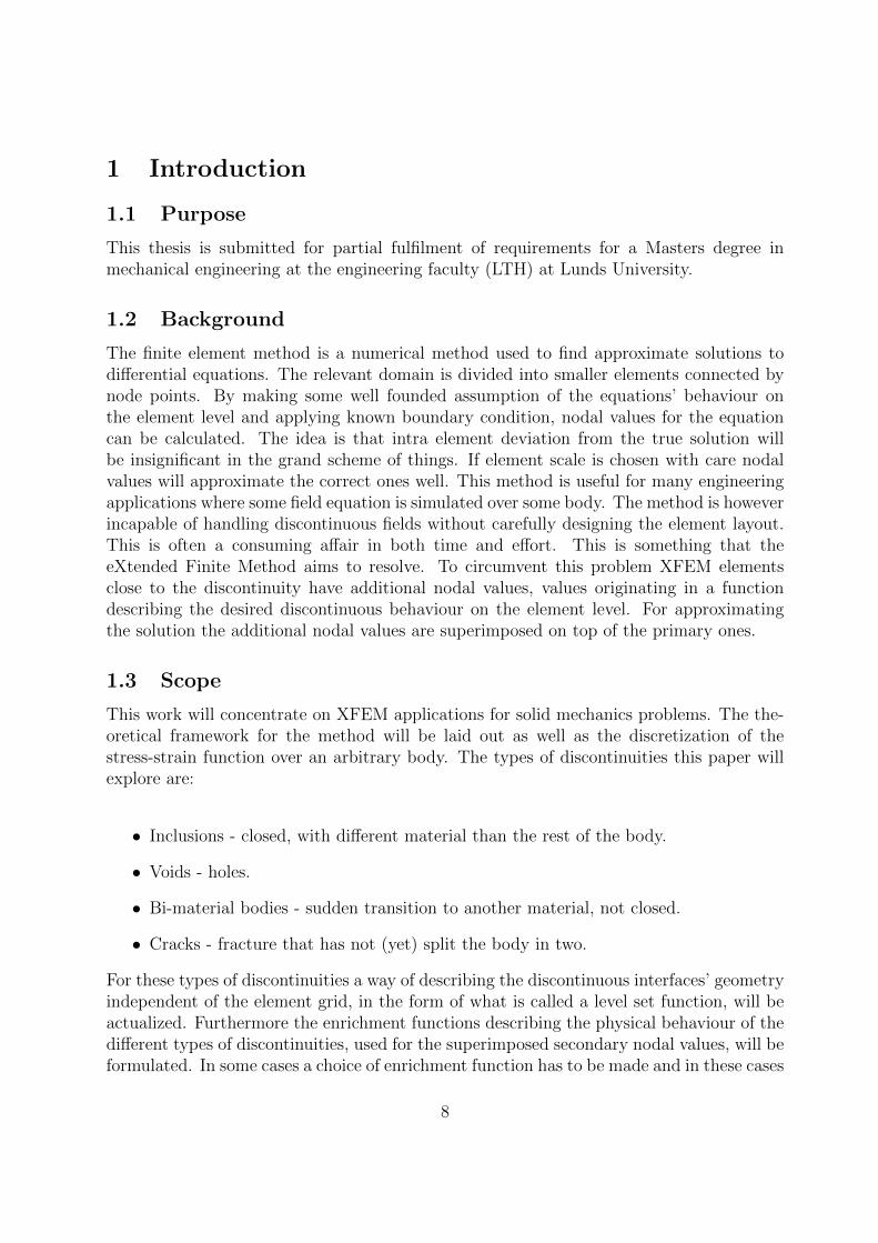
The finite element method is a numerical method used to find approximate solutions todifferential equations. The relevant domain is divided into smaller elements connected bynode points. By making some well founded assumption of the equations’ behaviour onthe element level and applying known boundary condition, nodal values for the equationcan be calculated. The idea is that intra element deviation from the true solution willbe insignificant in the grand scheme of things. If element scale is chosen with care nodalvalues will approximate the correct ones well. This method is useful for many engineeringapplications where some field equation is simulated over some body. The method is howeverincapable of handling discontinuous fields without carefully designing the element layout.This is often a consuming affair in both time and effort. This is something that theeXtended Finite Method aims to resolve. To circumvent this problem XFEM elementsclose to the discontinuity have additional nodal values, values originating in a functiondescribing the desired discontinuous behaviour on the element level. For approximatingthe solution the additional nodal values are superimposed on top of the primary ones.
1.3 Scope
This work will concentrate on XFEM applications for solid mechanics problems. The the-oretical framework for the method will be laid out as well as the discretization of thestress-strain function over an arbitrary body. The types of discontinuities this paper willexplore are:
• Inclusions - closed, with different material than the rest of the body.
• Voids - holes.
• Bi-material bodies - sudden transition to another material, not closed.
• Cracks - fracture that has not (yet) split the body in two.
For these types of discontinuities a way of describing the discontinuous interfaces’ geometryindependent of the element grid, in the form of what is called a level set function, will beactualized. Furthermore the enrichment functions describing the physical behaviour of thedifferent types of discontinuities, used for the superimposed secondary nodal values, will beformulated. In some cases a choice of enrichment function has to be made and in these cases
8
the practical foresight used to make this choice are discussed and explained. In parallelto the theoretical work the discussed items are implemented into the numerical computingenvironment MATLAB. The ambition level of this code is restricted to two dimensions,small strains and linear elasticity. This program is designed to work in tandem with thefinite element library CALFEM, developed by the department of solid- and structural-mechanics at LTH. While the code is intended to be used as a complete program where theuser only edits a set up file, individual files can be used as part of a library. This paper willevaluate the code in a series of test cases each corresponding to one or several topics in thetheoretical section. The evaluation involves reviewing performance but first and foremostis the achievement of a sufficient solution. In some cases a comparison with the standardFE-method with a specially designed grid can be made, elsewhere existing software is usedin the evaluation.
9
2 XFEM formulation and element integration
The purpose of this section is to introduce the enrichment associated with XFEM suchthat the structure of the finite element equation set is revealed. Later on details related tothe enrichment will be discussed.
2.1 Strong and weak form
The general formulation of the strong form for a body in equilibrium is as follows
∇σ + b = 0 (1)
Where σ is the stress tensor and b is the forces in the body, i.e. gravity. The next step isto consider a weak form, or a virtual energy form of the strong formulation of the body’sbehaviour. This can be done by multiplying with a arbitrary weight function, v, andintegrating over the whole body. The equation then takes the form∫
V
(∇v)Tσ dV =
∫S
vT t dS +
∫V
vTb dV (2)
where t is the surface loading and ∇ is the gradient operator acting on a vector in matrixformat.
2.2 XFEM formulation including enrichment.
The next step is the choice of the weight function, v. This is done with the so calledGalerkin’s method which is discussed in some detail in [1]. With this the weight function,with the enrichment considered, may be written as
v = Nc + Nenrq (3)
∇v = Bc + Benrq (4)
where c is the usual nodal quantities and q the part related to the enrichment term, thesewill be discussed in detail later on. In addition, N and B are the usual shape functionmatrix and the strain displacement matrix respectively. In the same manner Nenr and Benr
can be labelled but now related to the enrichment. Moreover, the differential operator wasincluded in eq.(4). Then all the terms in eq.(2) will be put to the left hand side, so we getan equality with zero. Insert eq.s(3) and (4), which describes the weight function, into (2).This will produce
cT [
∫V
BTσ dV
∫S
NT t dS
∫V
NTb dV ]
+ qT [
∫V
BTenrσ dV
∫S
NTenrt dS
∫V
NTenrb dV ] = 0 (5)
10
Since both c and q are arbitrary, eq.(5) can be divided into two parts as∫V
BTσ dV =
∫S
NT t dS
∫V
NTb dV (6)∫V
BTenrσ dV =
∫S
NTenrt dS
∫V
NTenrb dV (7)
We now have two equations which must both be fulfilled; one with the standard FEMequations and one which involve terms that comes from the enrichment. The next step isto find a constitute relation between stress and strain and to define and approximation forthe displacement, i.e.
σ = Dε (8)
where ε is the strain matrix defined as ε = ∇u, and
u = Nustd + Nenruxtra (9)
as previously, ustd are the standard nodal displacements and uxtra are related to the en-richment part. Inserted into eq.s (6) and (7) gives∫
V
BTDB dV ustd +
∫V
BTDBenr dV uxtra =
∫S
NT t dS
∫V
NTb dV (10)∫V
BTenrDB dV ustd +
∫V
BTenrDBenr dV uxtra =
∫S
NTenrt dS
∫V
NTenrb dV (11)
2.3 Defining the XFEM and FEM matrices
From eq.s (10) and (11) we can see that there will be four different types of stiffnessmatrices; one that is the normal stiffness matrix for FEM, combinations using both thestandard and enriched B-matrix, and one with only enrichment. The matrices involvinga combination of normal and enriched B-matrices are normally referred to as “blended”stiffness, this will be discussed later on. However it is noted that the equation system canbe written as [
Kstd Kblend
KTblend Kxtra
] [ustduxtra
]= F (12)
where
Kstd =
∫BTDB dV (13)
Kblend =
∫BTDBenr dV (14)
Kxtra =
∫BTenrDBenr dV (15)
For simplicity, in the discussion and examples it will be assumed that a 2-dimensionalgeometry is concerned. In addition, in the numerical parts it will be assumed that thereference mesh is defined by 4-node isoparametric elements.
11
3 Level Sets
3.1 Definition
As the idea of the XFEM is to capture discontinuities over some boundary without meshadjustment it is vital to be able to keep track of this interface. The most common way todo this is with a level set function. To visualize this let us imagine a domain Ω which isdivided into two separate, non zero sub-domains Ωa and Ωb. The boundary between Ωa
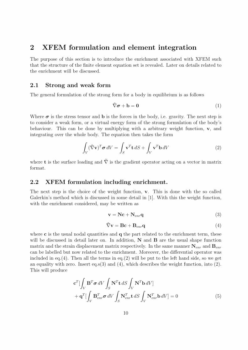
and Ωb is denoted Γ and represent the interface of interest, see Fig. 1. The level set φ(X)function has the property of:
φ(X) < 0 for X ∈ Ωb (16)
φ(X) > 0 for X ∈ Ωa (17)
φ(X) = 0 for X ∈ Γ (18)
Figure 1: Domain separated into sub-domains by an interface.
The sign of the level set function can now be used to reveal what part of the domaincertain coordinates X belong to, a zero value means the point of interest is located on theinterface itself. A helpful definition but an explicit function, chosen to fit some a prioriknown circumstances, is needed for implementation.
3.2 Moving Interface
Obviously the level set function has a time dependence when the interface of interest ismoving [1]. If one assumes knowledge of the initial conditions φ(X, t = 0), the interface
12
evolution function is given by the material time derivative
Dφ
Dt= 0 (19)
∂φ
∂t+ F ‖∇φ‖ = 0 (20)
Where F (X, t) is the interface’s normal outwards velocity. As the level set function is zeroat the interface the time derivative must be zero as well. The evolution function can berewritten with the velocity v
∂φ
∂t+ v · ∇φ = 0 (21)
In an practical situation, where the velocity field is given, an expression for updating thelevel set function can be derived with the time scheme of choice. A first order explicit timediscretization with an arbitrary spatial discretization is given as
φn+1 − φn
∆t= −φn,ivni (22)
φn+1 = φn −∆tφn,ivni (23)
The Courant-Friedrichs-Lewy stability condition [2] applies
∆tN∑i=1
vi∆xi
≤ Cmax (24)
Cmax = 1 (typically) (25)
This work will put little emphasis on this subject. It could however be noted that thisis a popular area of research, in particular for dynamic crack growth. The problem ofcrack growth direction have several possible solutions, for example finding a direction suchas modus II stress intensity factor is zero [10] maximizing the energy release rate locally.Other more general mixed mode methods exist as well [11]. These methods seem to matchexperimental results but are not perfectly understood and assumes ideal materials [12].This is somewhat problematic for real world applications as it ignores potentially crucialfactors such as small scale material imperfections.
3.3 Cracks and Other Curve Type Discontinuities
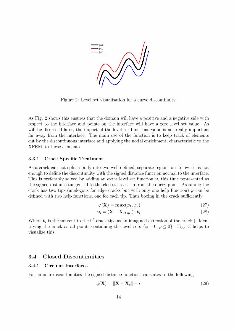
If the interface consist of some kind of curve a convenient choice of level set function is thesigned distance function. Let us define a vector d as the minimum distance from a point ofinterest X to the boundary XΓ. Using the outwards normal n to the interface the signeddistance function is defined as
φ(X) = d · n (26)
13
φ=0φ=1φ=-1
Figure 2: Level set visualisation for a curve discontinuity.
As Fig. 2 shows this ensures that the domain will have a positive and a negative side withrespect to the interface and points on the interface will have a zero level set value. Aswill be discussed later, the impact of the level set functions value is not really importantfar away from the interface. The main use of the function is to keep track of elementscut by the discontinuous interface and applying the nodal enrichment, characteristic to theXFEM, to these elements.
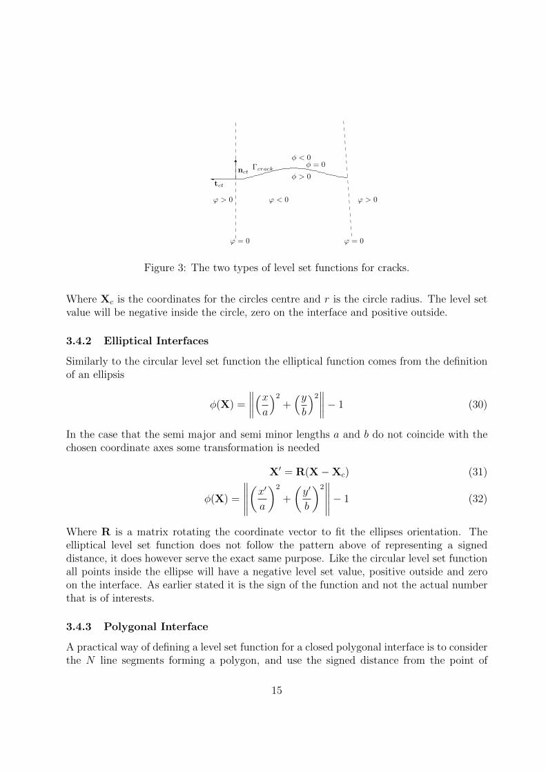
3.3.1 Crack Specific Treatment
As a crack can not split a body into two well defined, separate regions on its own it is notenough to define the discontinuity with the signed distance function normal to the interface.This is preferably solved by adding an extra level set function ϕ, this time represented asthe signed distance tangential to the closest crack tip from the query point. Assuming thecrack has two tips (analogous for edge cracks but with only one help function) ϕ can bedefined with two help functions, one for each tip. Thus boxing in the crack sufficiently
ϕ(X) = max(ϕ1, ϕ2) (27)
ϕi = (X−XcT ip i) · ti (28)
Where ti is the tangent to the ith crack tip (as an imagined extension of the crack ). Iden-tifying the crack as all points containing the level sets φ = 0, ϕ ≤ 0. Fig. 3 helps tovisualize this.
3.4 Closed Discontinuities
3.4.1 Circular Interfaces
For circular discontinuities the signed distance function translates to the following
φ(X) = ‖X−Xc‖ − r (29)
14
φ < 0
φ > 0nct
tct
φ = 0Γcrack
ϕ < 0
ϕ = 0 ϕ = 0
ϕ > 0 ϕ > 0
Figure 3: The two types of level set functions for cracks.
Where Xc is the coordinates for the circles centre and r is the circle radius. The level setvalue will be negative inside the circle, zero on the interface and positive outside.
3.4.2 Elliptical Interfaces
Similarly to the circular level set function the elliptical function comes from the definitionof an ellipsis
φ(X) =
∥∥∥∥(xa)2
+(yb
)2∥∥∥∥− 1 (30)
In the case that the semi major and semi minor lengths a and b do not coincide with thechosen coordinate axes some transformation is needed
X′ = R(X−Xc) (31)
φ(X) =
∥∥∥∥∥(x′
a
)2
+
(y′
b
)2∥∥∥∥∥− 1 (32)
Where R is a matrix rotating the coordinate vector to fit the ellipses orientation. Theelliptical level set function does not follow the pattern above of representing a signeddistance, it does however serve the exact same purpose. Like the circular level set functionall points inside the ellipse will have a negative level set value, positive outside and zeroon the interface. As earlier stated it is the sign of the function and not the actual numberthat is of interests.
3.4.3 Polygonal Interface
A practical way of defining a level set function for a closed polygonal interface is to considerthe N line segments forming a polygon, and use the signed distance from the point of
15
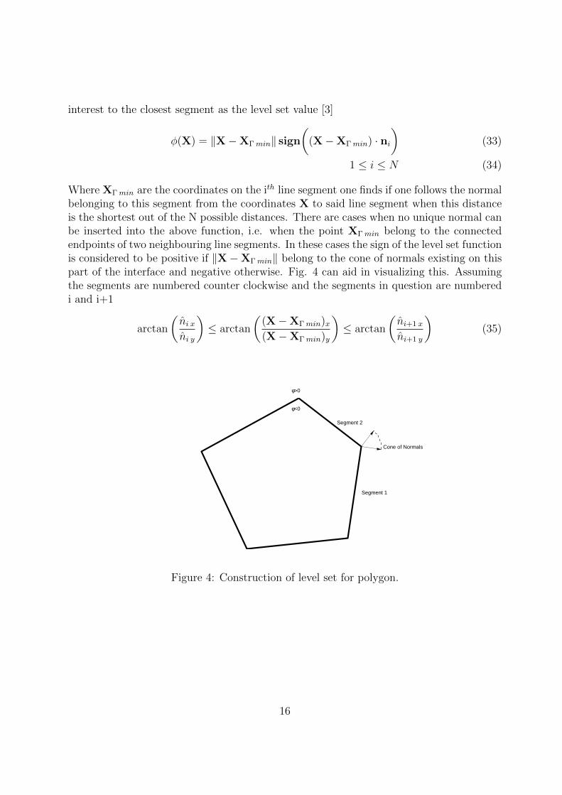
interest to the closest segment as the level set value [3]
φ(X) = ‖X−XΓmin‖ sign
((X−XΓmin) · ni
)(33)
1 ≤ i ≤ N (34)
Where XΓmin are the coordinates on the ith line segment one finds if one follows the normalbelonging to this segment from the coordinates X to said line segment when this distanceis the shortest out of the N possible distances. There are cases when no unique normal canbe inserted into the above function, i.e. when the point XΓmin belong to the connectedendpoints of two neighbouring line segments. In these cases the sign of the level set functionis considered to be positive if ‖X−XΓmin‖ belong to the cone of normals existing on thispart of the interface and negative otherwise. Fig. 4 can aid in visualizing this. Assumingthe segments are numbered counter clockwise and the segments in question are numberedi and i+1
arctan
(ni xni y
)≤ arctan
((X−XΓmin)x(X−XΓmin)y
)≤ arctan
(ni+1 x
ni+1 y
)(35)
Segment 1
Segment 2
Cone of Normals
φ>0
φ<0
Figure 4: Construction of level set for polygon.
16
4 Enrichment
4.1 Enrichment Function
The level set function provides knowledge of the location of the geometry. The remainingpart is to define the enrichment function in the XFEM approximation. The idea is toadd new degrees of freedom to the system and superimpose these on top of the standardFEM DOFs with some weight function. The task of the enrichment function is to supplythis weight in a fashion that captures the behaviour of the discontinuity. This assumesknowledge about the type of discontinuity, but it is hard to imagine a meaningful practicalsituation where this is not the case. As the behaviour of the discontinuity strongly relatesto the shape of the interface it is common to choose an enrichment function formulatedwith the level set function.
4.1.1 Partition of Unity
As the discontinuities are an uniquely local event some restriction must be applied. Apartition of unity is a set of functions which sum is one over a specified domain ΩPU∑
i
fi(X) = 1 (36)
∀X ∈ ΩPU (37)
The partition of unity method allows for the introduction of an arbitrary function [4], inour case enrichment function ψ(X), in the approximation. In FEM, usually, the shapefunctions gives this partition of unity and it is common practise to let shape functions playthe same role in the enriched part of the XFEM. This work will not deviate from this normbut it is noted that because the local approximation of the standard and enriched partof the XFEM formulation does not share a common origin it is not necessary to use thesame shape functions. A FEM approximation using a partition of unity function f , over adomain consisting of M nodes, could look like this
uaprox(X) =M∑I=1
fIustdI (38)
Adding the XFEM part to this, the domain has L enriched nodes starting with nodenumber L1
uaprox(X) =M∑I=1
fIustdI +
M∑I=1
fI
L∑J=L1
ψ(X)uxtraJ (39)
When introducing the shape functions, i.e. fI = NI this approximation becomes exclu-sively local
uaprox(XI) = ustdI + ψ(XI)uxtraI (40)
17
4.1.2 Strong vs. Weak Discontinuities
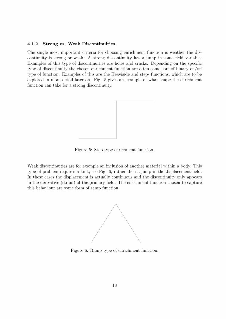
The single most important criteria for choosing enrichment function is weather the dis-continuity is strong or weak. A strong discontinuity has a jump in some field variable.Examples of this type of discontinuities are holes and cracks. Depending on the specifictype of discontinuity the chosen enrichment function are often some sort of binary on/offtype of function. Examples of this are the Heaviside and step- functions, which are to beexplored in more detail later on. Fig. 5 gives an example of what shape the enrichmentfunction can take for a strong discontinuity.
Figure 5: Step type enrichment function.
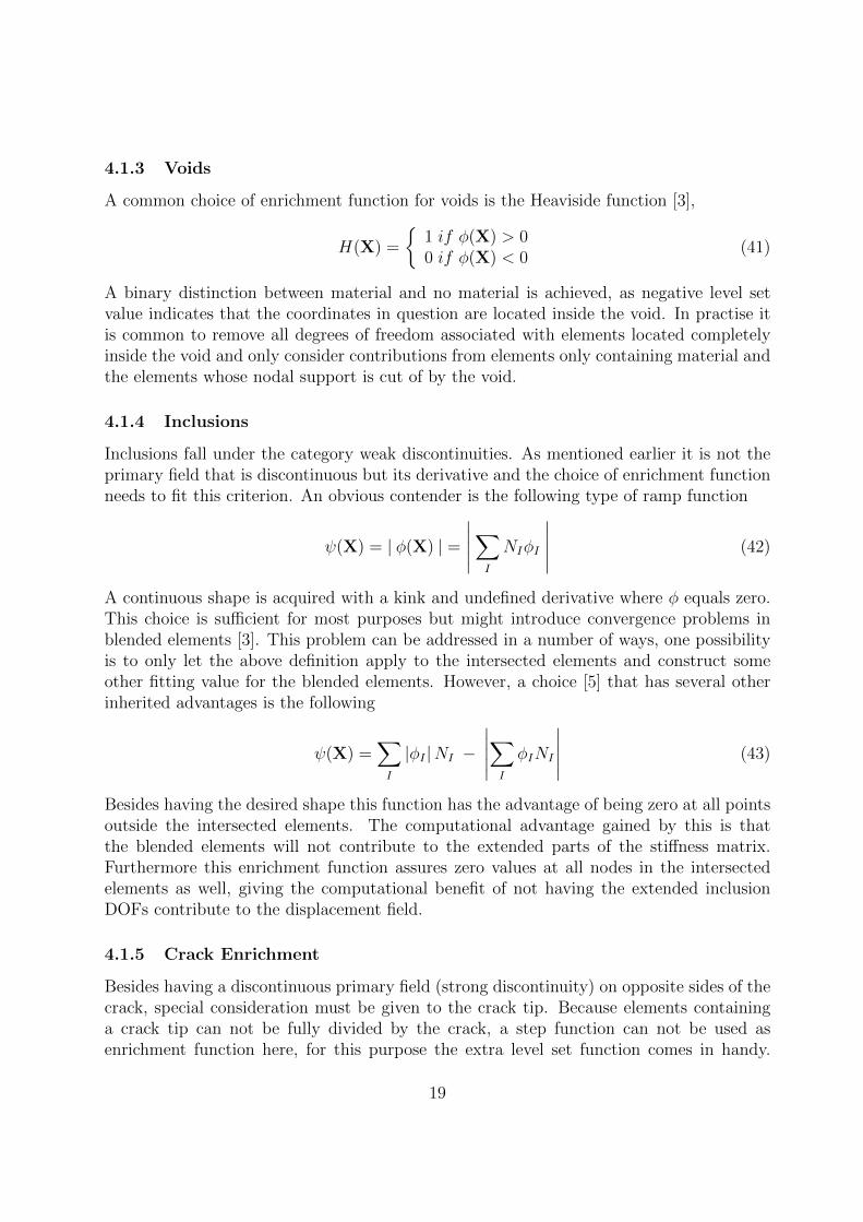
Weak discontinuities are for example an inclusion of another material within a body. Thistype of problem requires a kink, see Fig. 6, rather then a jump in the displacement field.In these cases the displacement is actually continuous and the discontinuity only appearsin the derivative (strain) of the primary field. The enrichment function chosen to capturethis behaviour are some form of ramp function.
Figure 6: Ramp type of enrichment function.
18
4.1.3 Voids
A common choice of enrichment function for voids is the Heaviside function [3],
H(X) =
1 if φ(X) > 00 if φ(X) < 0
(41)
A binary distinction between material and no material is achieved, as negative level setvalue indicates that the coordinates in question are located inside the void. In practise itis common to remove all degrees of freedom associated with elements located completelyinside the void and only consider contributions from elements only containing material andthe elements whose nodal support is cut of by the void.
4.1.4 Inclusions
Inclusions fall under the category weak discontinuities. As mentioned earlier it is not theprimary field that is discontinuous but its derivative and the choice of enrichment functionneeds to fit this criterion. An obvious contender is the following type of ramp function
ψ(X) = | φ(X) | =
∣∣∣∣∣∑I
NIφI
∣∣∣∣∣ (42)
A continuous shape is acquired with a kink and undefined derivative where φ equals zero.This choice is sufficient for most purposes but might introduce convergence problems inblended elements [3]. This problem can be addressed in a number of ways, one possibilityis to only let the above definition apply to the intersected elements and construct someother fitting value for the blended elements. However, a choice [5] that has several otherinherited advantages is the following
ψ(X) =∑I
|φI |NI −
∣∣∣∣∣∑I
φINI
∣∣∣∣∣ (43)
Besides having the desired shape this function has the advantage of being zero at all pointsoutside the intersected elements. The computational advantage gained by this is thatthe blended elements will not contribute to the extended parts of the stiffness matrix.Furthermore this enrichment function assures zero values at all nodes in the intersectedelements as well, giving the computational benefit of not having the extended inclusionDOFs contribute to the displacement field.
4.1.5 Crack Enrichment
Besides having a discontinuous primary field (strong discontinuity) on opposite sides of thecrack, special consideration must be given to the crack tip. Because elements containinga crack tip can not be fully divided by the crack, a step function can not be used asenrichment function here, for this purpose the extra level set function comes in handy.
19
First lets use the level set functions φ and ϕ to define some help variables to make thecrack tip enrichment a little more straightforward
θ = arctanϕ
φ(44)
r =√φ2 + ϕ2 (45)
Without diving too deep into the realm of fracture mechanics it can be stated that for linearelastic fracture mechanics the displacement field near the crack tip [6], can be written as
ux =KI
2µ
√r
2πcos
θ
2
(κ− 1 + 2 sin2 θ
2
)+KII
2µ
√r
2πsin
θ
2
(κ+ 1 + 2 cos2 θ
2
)(46)
uy =KI
2µ
√r
2πsin
θ
2
(κ+ 1− 2 cos2 θ
2
)−KII
2µ
√r
2πcos
θ
2
(κ− 1− 2 sin2 θ
2
)(47)
Where KI and KII are the mode 1 and 2 stress intensity factors. The Koslov constant isdefined as
κ = 3− 4ν (plane stress) (48)
κ =3− ν1 + ν
(plane strain) (49)
It can be shown that the crack tip displacement field is contained by four functions [7],
γ(r, θ) =
√r cos θ
2
√r sin θ
2
√r sin θ
2sin θ
√r cos θ
2sin θ
(50)
Furthermore, it is possible to combine these functions for the crack tip enrichment[6]. Un-fortunately this enrichment requires that one new degree of freedom per node is introducedfor each of these four functions. On the other hand the problem of crack tip enrichmentis solved and only two elements in a domain can contain a crack tip (one for edge cracks).The functions used are not discontinuous on their own, only when combined with the helpvariables defined with the level set functions the desired properties show up. If we considera domain where the part of the domain containing crack tip enrichment is denoted Ωct and
20

the part of with normal crack enrichment ΩH , the XFEM displacement approximation forsuch a case would read as
uaprox(XI) = ustdI +H(XI)uxtraI (51)
forI ∈ ΩH
uaprox(XI) = ustdI + γ1(XI)uxtra1I + γ2(XI)u
xtra2I + γ3(XI)u
xtra3I + γ4(XI)u
xtra4I (52)
forI ∈ Ωct
Note that no node can have with both heaviside and crack tip enrichment.
21
5 Test Case 1: Circular inclusion
5.1 Preprocessing and Set Up
5.1.1 Geometry
A relative simple start problem was chosen, in part to simplify validation and troubleshoot-ing but mainly for the author to explore the most essential aspects of XFEM. The problemwas decided to be a 2D quadratic plate with a circular inclusion of another material. Thiswas implemented for a plane stress case with the boundary conditions that the bottomedge of the plate was locked in place in vertical direction resting on rollers, and the leftmost corner of this edge was also locked in place in the horizontal direction. The force wasapplied on the plates top edge and equally distributed along this edge.
5.1.2 Level Set
The implemented level set function was the following:
φ(X) = |X−Xc| − r (53)
Where φ(X) is the level set value at coordinates X. Xc is the centre coordinates for thecircular inclusion and r is the radius of the inclusion. These values were stored at all nodesfor later use. To extract the level set value at arbitrary coordinates the element shapefunctions are used, since the used shape functions are for first order interpolation they willnot be able to fully capture the circle. Instead the extracted interface will have the shapeof a polygon. This has no impact on elements that are not cut by the interface. Elementscontaining the interface will be cut up in polygons anyway for integrating purposes.
5.2 Main Calculation
5.2.1 Enrichment Function
The implemented enrichment function is:
ψ(X) =4∑I=1
|φI |N(X)I − |4∑I=1
φIN(X)I | (54)
The enrichment function ψ at coordinates X is evaluated as a combination of nodal levelset values and the shape functions. Compared to other choices for enrichment functionsthis has two major advantages. As the enrichment function has a zero value outside cutelements as well as in cut element nodes there will be no contribution to the stiffnessmatrix in an element that are not cut by the interface and the displacements evaluated atthe nodes will not have any extra contribution either.
22
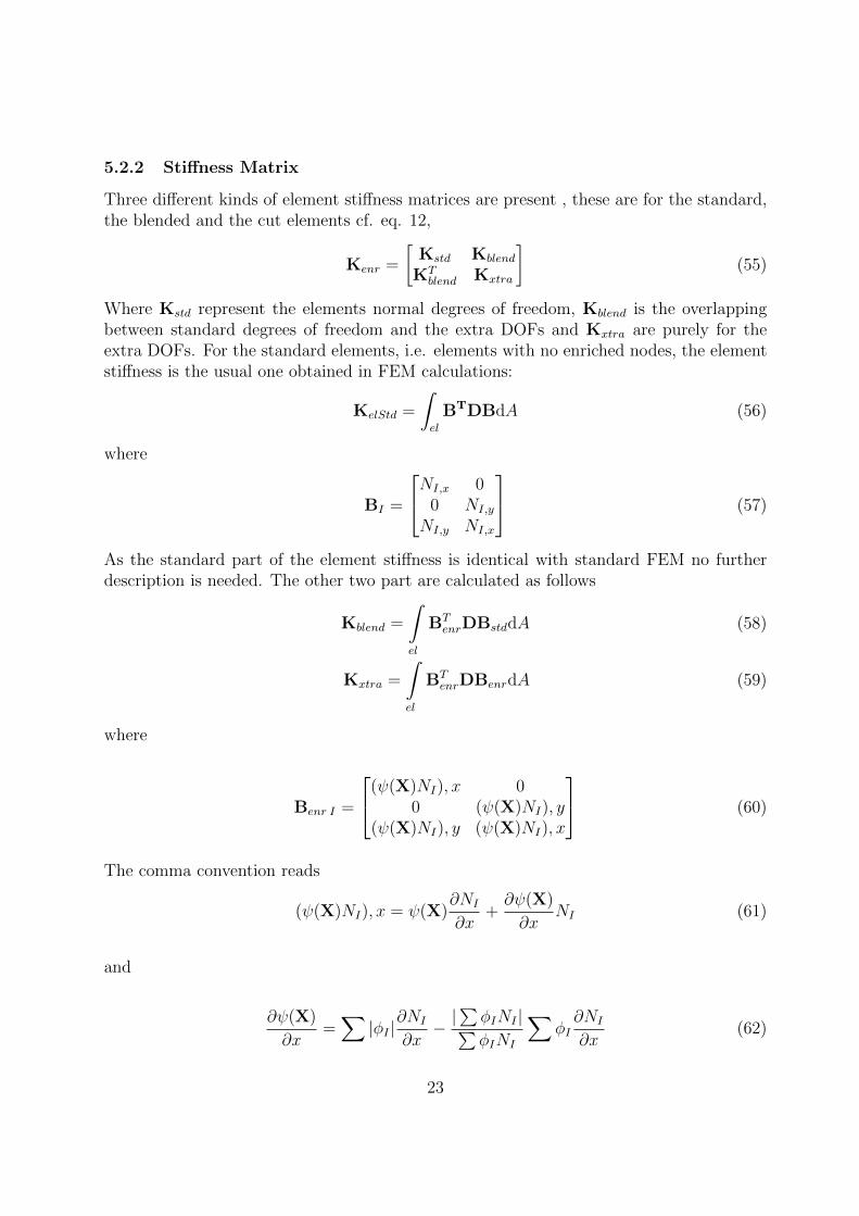
5.2.2 Stiffness Matrix
Three different kinds of element stiffness matrices are present , these are for the standard,the blended and the cut elements cf. eq. 12,
Kenr =
[Kstd Kblend
KTblend Kxtra
](55)
Where Kstd represent the elements normal degrees of freedom, Kblend is the overlappingbetween standard degrees of freedom and the extra DOFs and Kxtra are purely for theextra DOFs. For the standard elements, i.e. elements with no enriched nodes, the elementstiffness is the usual one obtained in FEM calculations:
KelStd =
∫el
BTDBdA (56)
where
BI =
NI,x 00 NI,y
NI,y NI,x
(57)
As the standard part of the element stiffness is identical with standard FEM no furtherdescription is needed. The other two part are calculated as follows
Kblend =
∫el
BTenrDBstddA (58)
Kxtra =
∫el
BTenrDBenrdA (59)
where
Benr I =
(ψ(X)NI), x 00 (ψ(X)NI), y
(ψ(X)NI), y (ψ(X)NI), x
(60)
The comma convention reads
(ψ(X)NI), x = ψ(X)∂NI
∂x+∂ψ(X)
∂xNI (61)
and
∂ψ(X)
∂x=∑|φI |
∂NI
∂x− |∑φINI |∑φINI
∑φI∂NI
∂x(62)
23
For blended elements, i.e. elements neighbouring to the elements cut by the interface andthus inherits enriched nodes, the chosen enrichment function conveniently makes sure allextra parts have a zero value. For fully enriched (cut) elements two different material prop-erties are present. Therefore the code divides the element into triangles trying to capturethe circular interface as true as possible where each triangle have only one constitutive ma-trix D The full integral is calculated as the sum of all partial integrals over each individualtriangle, c.f. Appendix A for numerical integration.
5.2.3 Displacement Field
The equation system to be solved:[Kstd Kblend
KTblend Kxtra
] [ustduxtra
]= Fexternal (63)
The displacement of a node is the sum of the standard displacement and the extra displace-ment weighted with the enrichment function. However the chosen enrichment function isonce again found to be extremely practical as it is zero at the nodes, ustd gives the correctdisplacements directly.
5.3 Post Processing
5.3.1 Stress Calculation
The stress is calculated at all nodes according to:
σ = Dε (64)
σ = D∇u (65)
With the element interpolation approximation applied this translates to:
σ = DBstdustd (66)
for non enriched elements and
σ = D[
Bstd Benrch
] [ ustduxtra
](67)
for enriched elements. For non enriched elements the code will use the element coordinates( [ξ1 η1] = [−1 − 1], coordinates in the isoparametric domain ) for a corner and calculatethe stresses at the nodes with the appropriate D matrix and store these.
A program developed by Matthew Pais at University of Florida[8] was used for com-parison in which enriched elements are treated the same way as non enriched ones. Inthis implementation elements cut by the level set interface are once again divided intotriangles creating pseudo elements where some of the new pseudo nodes does not coincide
24
with the original elements nodes. The calculation then proceeds using the parent elementcoordinates to extract the values at the pseudo nodes. This somewhat cumbersome proce-dure was implemented in hopes of capturing the stresses at the interface in a more precisemanner. As the new pseudo elements are considered to be either the positive or negativeside of the interface average nodal stresses can be calculated for the positive and negativeside separately. When displaying the stresses the code makes sure no interpolation takesplace between elements on opposite sides of the interface before plotting in a contour plot.
5.3.2 Validation
The implemented code was run on an identical set up as Pais code with the followingproperties
E-modulus positive side 69×109 GPaE-modulus negative side 205×109 GPaPoissons ratio pos. side 0.33Poissons ratio neg. side 0.3Inclusion radius 0.45 mApplied force magnitude 1 MNInclusion placement centre of platePlate dimensions 2×2 mThickness 1m
A plate of a steel like material have an inclusion of an aluminium like material. Paisprogram, Fig. 8, and the implemented code produce very similar results. When both thiscode and Pais code are set up to use 80×80 elements the maximal difference is in the orderof 10−6 %. As the result gives reasonable values and for all intents and purposes assumesan expected symmetric stress distribution the author will consider these results adequate.To examine whether the result is grid independent is more complicated. As the splittinginto triangles technique used will effectively approximate the inclusion as a polygon, theapproximation will become better and better as the number of elements increase and theinclusion will change shape with this increase. The simulation depicted in Fig. 7 is run on3025 elements. No practical difference was found when running with 6400 elements. Asthere are no practical application intended for this simulation this result will be consideredsufficient. It should be mentioned that the stress concentration found along the boundaryin Figs. 7 and 8 are a result of numerical issues and is not consistent with what wouldbe expected from a theoretical point of view. The code can not perfectly account for thediscontinuity when calculating stress in nodes on the boundary. The more lopsided and/orextreme angled an element is cut by the interface the worse the approximation used to findintra element level set values works. In extreme cases it has been found that error in thisapproximation has been in the order of 10% of the element length.
25
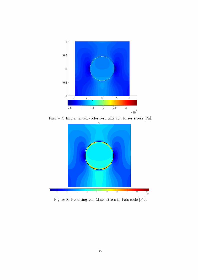
Figure 7: Implemented codes resulting von Mises stress [Pa].σvm
0.6 0.8 1 1.2 1.4 1.6 1.8 2 2.2 2.4
x 106
Figure 8: Resulting von Mises stress in Pais code [Pa].
26

6 Test Case 2: Circular Hole
6.1 Preprocessing and Set Up
6.1.1 Geometry
Very similar to test case 1, square domain with circular hole instead of inclusion. Planestress thickness was 0.2m. Size of square domain was 2×2 m and radius of the centrallylocated hole was 0.45 m. A variety of grid sizes were tested, with the properties
E-modulus positive side 69×109 GPaPoissons ratio pos. side 0.33Hole radius 0.45 mApplied force magnitude 1 MNInclusion placement centre of platePlate dimensions 2×2 mPlate thickness 0.2 m
The boundary conditions were the same as for test case 1 i.e. bottom edge locked inthe vertical direction and bottom left is locked in horizontally as well. The force wasplaced along the top edge, evenly distributed pulling the plate.
6.1.2 Level Set
The used level set function is identical to the one used in test case 1, i.e.
φ(X) = |X−Xc| − r (68)
6.1.3 Enrichment Function
Again identical to test case 1, the enrichment is taken as
ψ(X) =4∑I=1
|φI |N(X)I −4∑I=1
|φIN(X)I | (69)
The main difference between test case one and two are what constitutive matrices are used.
6.1.4 Stiffness Matrix
As in test case one, when integrating over an element cut by the discontinuity a differentconstitutive matrix is used depending on which side of the interface the current gauss pointis located. In this case the negative level set side has a zero-matrix as constitutive matrix.
6.1.5 Displacement Field
As in test case one, treatment is identical to 5.2.3
27
6.2 Post Processing
6.2.1 Stress Calculation
The treatment is analogous with test case 1 with the exception that the constitutive matrixis a zero matrix in the void region.
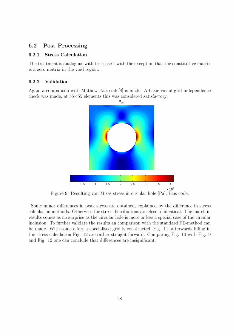
6.2.2 Validation
Again a comparison with Mathew Pais code[8] is made. A basic visual grid independencecheck was made, at 55×55 elements this was considered satisfactory.
σvm
0 0.5 1 1.5 2 2.5 3 3.5 4
x 105
Figure 9: Resulting von Mises stress in circular hole [Pa], Pais code.
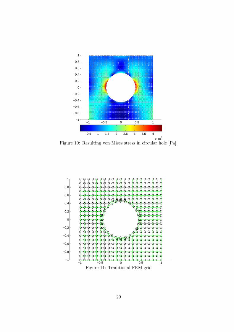
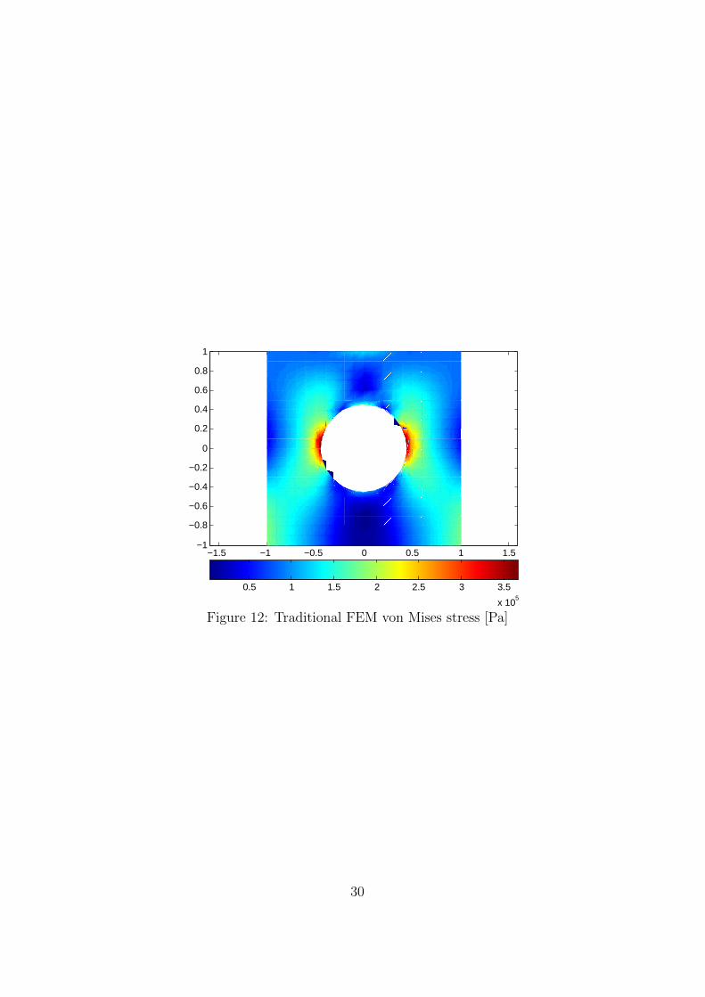
Some minor differences in peak stress are obtained, explained by the difference in stresscalculation methods. Otherwise the stress distributions are close to identical. The match inresults comes as no surprise as the circular hole is more or less a special case of the circularinclusion. To further validate the results an comparison with the standard FE-method canbe made. With some effort a specialised grid is constructed, Fig. 11, afterwards filling inthe stress calculation Fig. 12 are rather straight forward. Comparing Fig. 10 with Fig. 9and Fig. 12 one can conclude that differences are insignificant.
28
−1 −0.5 0 0.5 1−1
−0.8
−0.6
−0.4
−0.2
0
0.2
0.4
0.6
0.8
1
0.5 1 1.5 2 2.5 3 3.5 4
x 105
Figure 10: Resulting von Mises stress in circular hole [Pa].
−1 −0.5 0 0.5 1−1
−0.8
−0.6
−0.4
−0.2
0
0.2
0.4
0.6
0.8
1
Figure 11: Traditional FEM grid
29
−1.5 −1 −0.5 0 0.5 1 1.5−1
−0.8
−0.6
−0.4
−0.2
0
0.2
0.4
0.6
0.8
1
0.5 1 1.5 2 2.5 3 3.5
x 105
Figure 12: Traditional FEM von Mises stress [Pa]
30
7 Test Case 3: Polygonal Level Set Boundary
7.1 Preprocessing and Set Up
7.1.1 Geometry
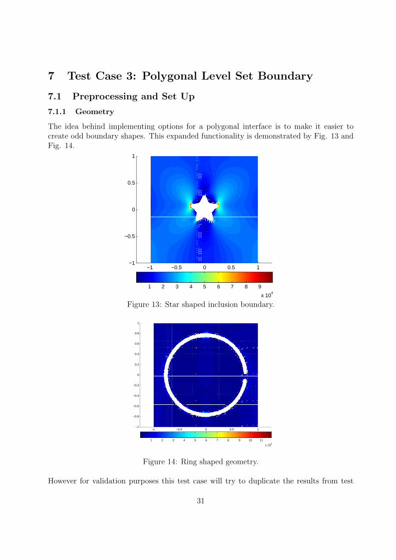
The idea behind implementing options for a polygonal interface is to make it easier tocreate odd boundary shapes. This expanded functionality is demonstrated by Fig. 13 andFig. 14.
−1 −0.5 0 0.5 1−1
−0.5
0
0.5
1
1 2 3 4 5 6 7 8 9
x 104
Figure 13: Star shaped inclusion boundary.
−1 −0.5 0 0.5 1−1
−0.8
−0.6
−0.4
−0.2
0
0.2
0.4
0.6
0.8
1
1 2 3 4 5 6 7 8 9 10 11
x 105
Figure 14: Ring shaped geometry.
However for validation purposes this test case will try to duplicate the results from test
31
case 1 and 2, circular inclusion and hole. The circle will be represented by a series ofline segments where endpoints always meet on the circle circumference. Other then theinterface set up geometry and load settings will match those of the other two test cases.
7.1.2 Level set
The implemented level set function was a signed distance from the coordinates of interest tothe interface defined in section 3.4.3. A quite computational heavy technique for calculatingthis was implemented. From each node and every line segment, the intersecting pointbetween a line along the line segments outwards normal and the node and the line segmentitself was calculated. If no such point could be found the closest line segment end pointwas chosen to account for cone of normals cases, see Fig. 4.
7.2 Main Calculation
7.2.1 Enrichment Function
The implemented enrichment function is the same as in examples 1 and 2, i.e.
ψ(X) =4∑I=1
|φI |N(X)I −4∑I=1
|φIN(X)I | (70)
This to ensure that the desired result should be comparable with the previous test cases.
7.2.2 Stiffness Matrix
Follows what was outlined in example 1.
7.2.3 Displacement Field
Same as for example 1.
7.3 Post Processing
7.3.1 Stress Calculation
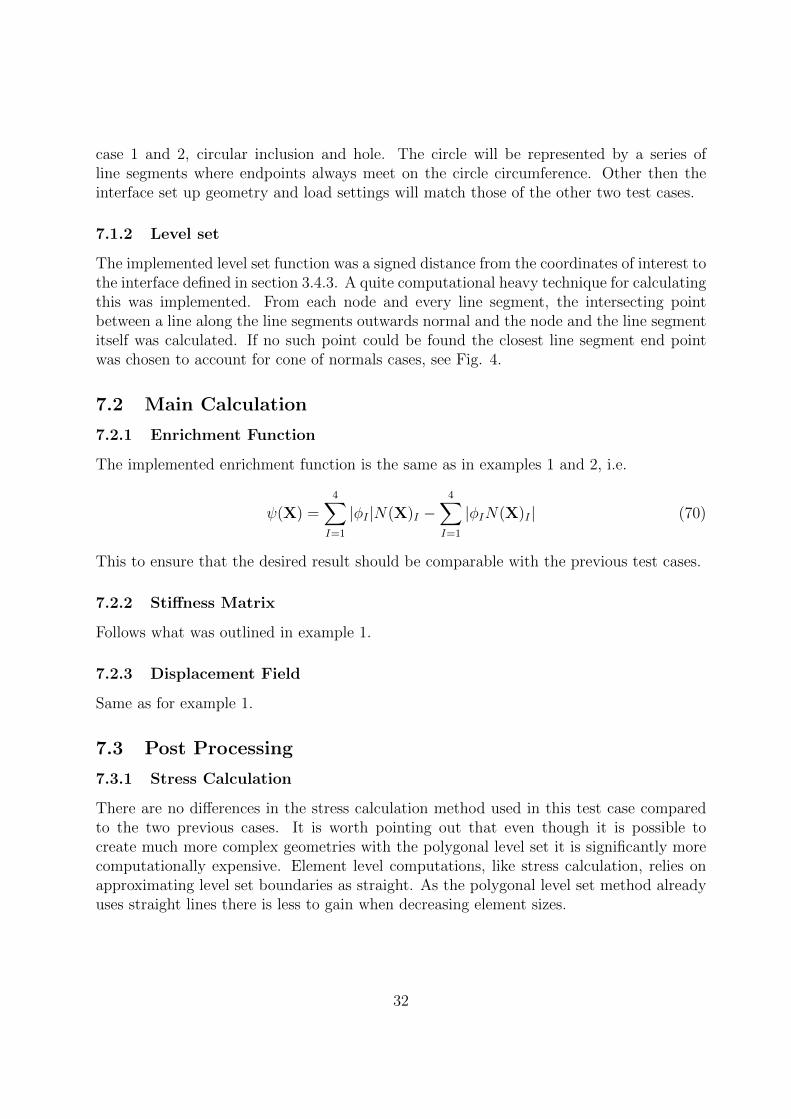
There are no differences in the stress calculation method used in this test case comparedto the two previous cases. It is worth pointing out that even though it is possible tocreate much more complex geometries with the polygonal level set it is significantly morecomputationally expensive. Element level computations, like stress calculation, relies onapproximating level set boundaries as straight. As the polygonal level set method alreadyuses straight lines there is less to gain when decreasing element sizes.
32
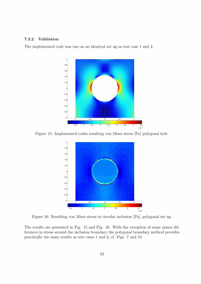
7.3.2 Validation
The implemented code was run on an identical set up as test case 1 and 2.
−1 −0.5 0 0.5 1−1
−0.8
−0.6
−0.4
−0.2
0
0.2
0.4
0.6
0.8
1
0.5 1 1.5 2 2.5 3 3.5 4 4.5
x 105
Figure 15: Implemented codes resulting von Mises stress [Pa] polygonal hole.
−1 −0.5 0 0.5 1−1
−0.8
−0.6
−0.4
−0.2
0
0.2
0.4
0.6
0.8
1
0.5 1 1.5 2 2.5 3 3.5
x 106
Figure 16: Resulting von Mises stress in circular inclusion [Pa], polygonal set up.
The results are presented in Fig. 15 and Fig. 16. With the exception of some minor dif-ferences in stress around the inclusion boundary the polygonal boundary method providespractically the same results as test cases 1 and 2, cf. Figs. 7 and 10.
33
8 Test Case 4: Straight Bimaterial Boundary
8.1 Preprocessing and Set up
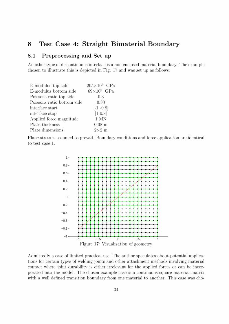
An other type of discontinuous interface is a non enclosed material boundary. The examplechosen to illustrate this is depicted in Fig. 17 and was set up as follows:
E-modulus top side 205×109 GPaE-modulus bottom side 69×109 GPaPoissons ratio top side 0.3Poissons ratio bottom side 0.33interface start [-1 -0.8]interface stop [1 0.8]Applied force magnitude 1 MNPlate thickness 0.08 mPlate dimensions 2×2 m
Plane stress is assumed to prevail. Boundary conditions and force application are identicalto test case 1.
−1 −0.5 0 0.5 1−1
−0.8
−0.6
−0.4
−0.2
0
0.2
0.4
0.6
0.8
1
Figure 17: Visualization of geometry
Admittedly a case of limited practical use. The author speculates about potential applica-tions for certain types of welding joints and other attachment methods involving materialcontact where joint durability is either irrelevant for the applied forces or can be incor-porated into the model. The chosen example case is a continuous square material matrixwith a well defined transition boundary from one material to another. This case was cho-
34
sen to be similar to other test cases and to demonstrate a different type of implementationmethod.
8.1.1 Geometry
As for the other examples the domain is chosen as a 2×2m plate, this time with a thicknessof 0.08m and a diagonal bi-material interface. A symmetrical element grid is placed overthe domain with no consideration to interface placement. The test case was implementedfor both 20×20 and 201×201 elements to study grid dependency issues.
8.1.2 Level Set
For a non enclosed boundary the level set description found in 3.3.1 is used, however asthe interface spans across the entire grid there is no need to keep track of endpoints andposition normal to the boundary. The level set function used is the signed tangentialdistance, of the lowest value, from the coordinates of interest to the interface. In this casethe interface is a straight line thus all points on the interface share a single normal n. Tocalculate the level set φ for a given point P given two points on the interface A and B thefollowing equation system is solved
A + α(B−A) = P + φn. (71)
Where α is a factor of no interest to the calculation and can be eliminated. Assuming(Bx−Ax) (By−Ay) 6= 0, otherwise special consideration must be taken to avoid divisionby zero (
Px−Ax
Bx−Ax− Py−Ay
By−Ay
Bx−Ax
By−Ay+ By−Ay
Bx−Ax
)|AB | = φ (72)
8.2 Main Calculation
No different from earlier test cases.
8.2.1 Enrichment Function
The level set function is the same as for the previous cases the enrichment is
ψ(X) =4∑I=1
|φI |N(X)I −4∑I=1
|φIN(X)I | (73)
8.2.2 Stiffness Matrix
As the enrichment function is the same as previously description follows from test case 1.
35
8.2.3 Displacement field
As before the system of equations provides the standard and enriched displacements afterwhich enriched displacements needs to be weighted and super positioned on top of thestandard ones for the desired results.
8.3 Post Processing
Follows what was outlined in test case 1.
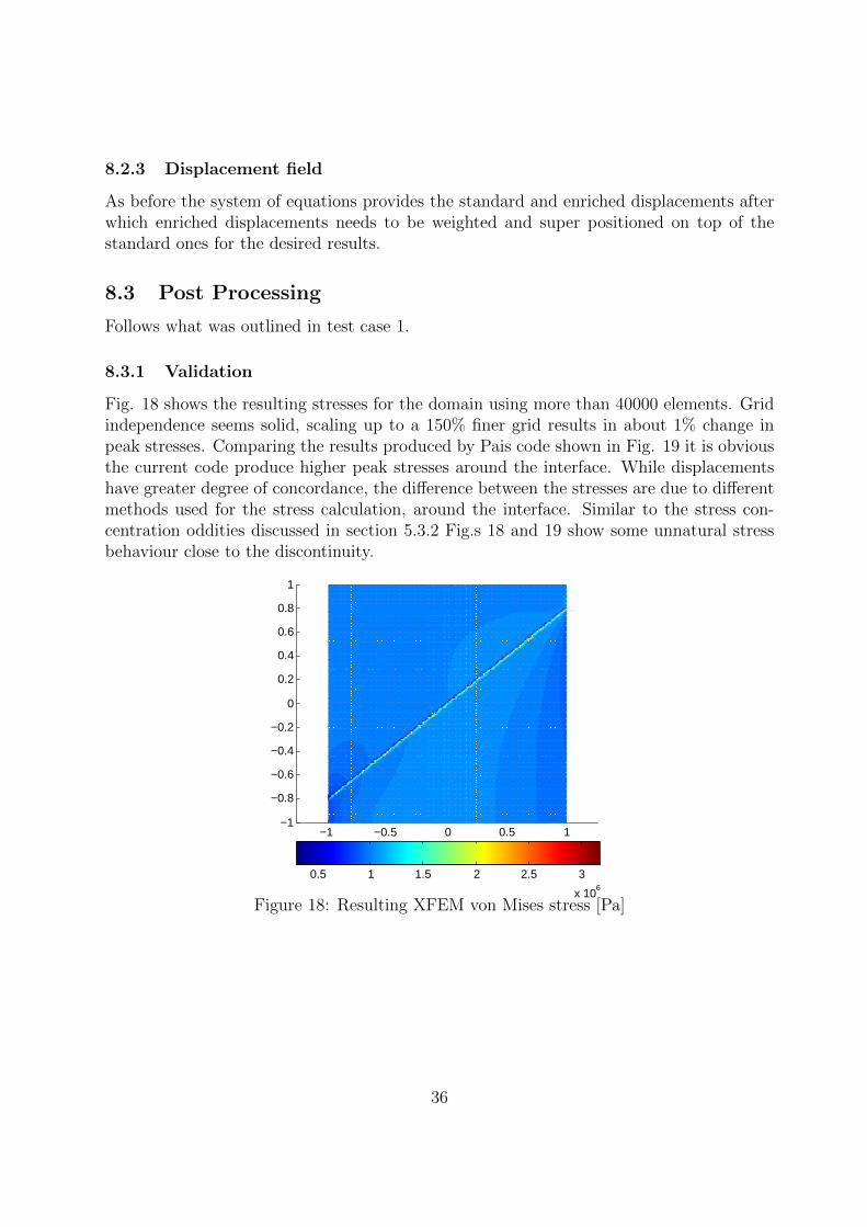
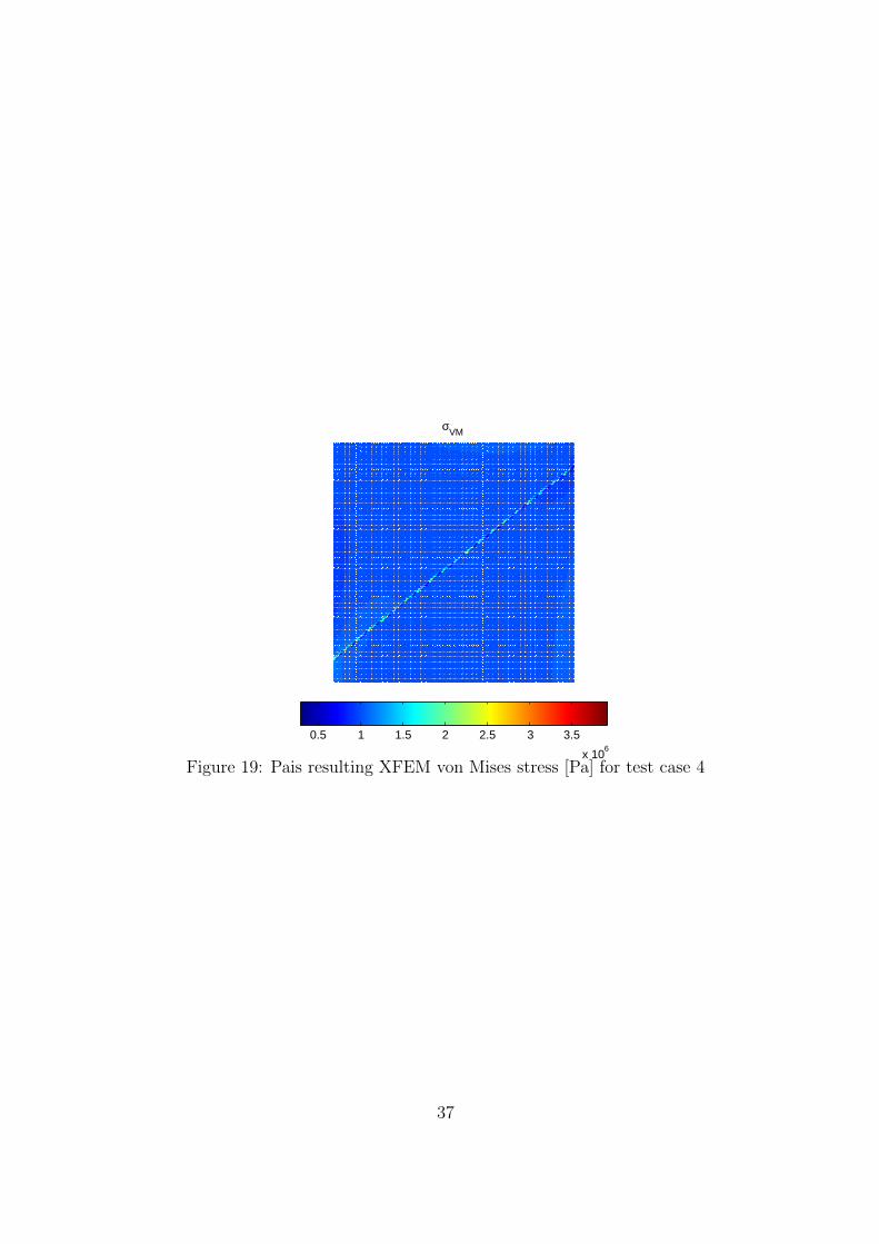
8.3.1 Validation
Fig. 18 shows the resulting stresses for the domain using more than 40000 elements. Gridindependence seems solid, scaling up to a 150% finer grid results in about 1% change inpeak stresses. Comparing the results produced by Pais code shown in Fig. 19 it is obviousthe current code produce higher peak stresses around the interface. While displacementshave greater degree of concordance, the difference between the stresses are due to differentmethods used for the stress calculation, around the interface. Similar to the stress con-centration oddities discussed in section 5.3.2 Fig.s 18 and 19 show some unnatural stressbehaviour close to the discontinuity.
−1 −0.5 0 0.5 1−1
−0.8
−0.6
−0.4
−0.2
0
0.2
0.4
0.6
0.8
1
0.5 1 1.5 2 2.5 3
x 106
Figure 18: Resulting XFEM von Mises stress [Pa]
36
σVM
0.5 1 1.5 2 2.5 3 3.5
x 106
Figure 19: Pais resulting XFEM von Mises stress [Pa] for test case 4
37
9 Test Case 5: Straight Crack
9.1 Preprocessing and Set up
9.1.1 Geometry
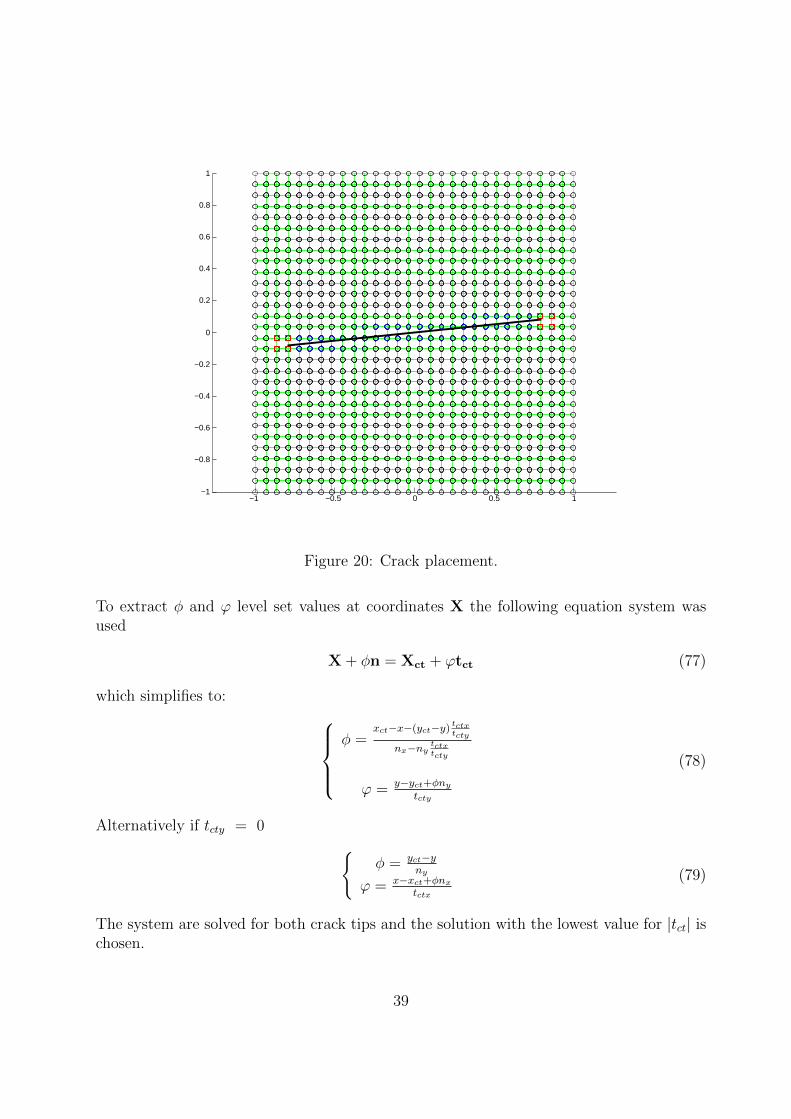
Again a square domain, 2×2 m, was chosen because it made the set up easy. A fairlycommon application could be a crack in a thin plate with a load trying to force the crackopen orthogonally, to the crack direction. Plain stress was assumed. To avoid symmetrythe crack was slightly tilted. If the centre of the plate is considered to be origin for astandard Cartesian coordinate system with the y-direction pointing directly upwards theboth crack tips was placed at the points [-0.8 -0.08] and [0.8 0.08]. Fig. 20 shows how thecrack was placed as well as potential enriched nodes for a 29×29 grid, cracktip enrichmentare red and Heaviside enrichment are blue. The test case is summarized by:
E-modulus 69×109 GPaPoissons ratio 0.33Left crack tip coordinates x=-0.8, y=-0.08Right crack tip coordinates x=0.8, y=0.08Plate dimensions 2×2 mPlane stress thickness 0.08 mForce magnitude 1MN
Boundary conditions and force distribution are identical to those of test case one.
9.1.2 Level Set
As described in subsection 3.3.1 when dealing with a crack it is necessary to have two levelset function. One to describe a points location perpendicular to the crack (above/below)and one level set function to describe the points spatial relation to the crack in the directionparallel to the crack (inside/outside a crack tip). These both functions are named the φand ϕ function, respectively. To calculate these values the code first calculates a normalfor the crack and two outwards pointing tangents, one for each crack tip. Then the codeloops over all grid points and traces a line parallel to the normal until it intersects theextended line created by the crack. The φ level set value is the length of this line, the signis determined by checking if the traced line follows the normal or the negative normal. Thecode then follows the same principle for the both crack tip tangents and chooses the onewhich results in the shortest vector as the ϕ level set value
n =1
|Xct2 −Xct1|
[0 −11 0
](Xct2 −Xct1) (74)
tct1 =Xct2 −Xct1
|Xct2 −Xct1|(75)
tct2 =Xct1 −Xct2
|Xct1 −Xct2|(76)
38
−1 −0.5 0 0.5 1−1
−0.8
−0.6
−0.4
−0.2
0
0.2
0.4
0.6
0.8
1
Figure 20: Crack placement.
To extract φ and ϕ level set values at coordinates X the following equation system wasused
X + φn = Xct + ϕtct (77)
which simplifies to: φ =
xct−x−(yct−y)tctxtcty
nx−nytctxtcty
ϕ = y−yct+φny
tcty
(78)
Alternatively if tcty = 0 φ = yct−y
ny
ϕ = x−xct+φnx
tctx
(79)
The system are solved for both crack tips and the solution with the lowest value for |tct| ischosen.
39
9.2 Main Calculation
9.2.1 Enrichment Function
Two types of enrichments are needed Heaviside and cracktip. Heaviside enrichment ac-counts for the loss of connection between nodes in an element cut by the crack, cracktipenrichment is used for capturing special crack tip behaviour. The Heaviside enrichmentneeds to be slightly modified compared to a hole set up. In a hole case the enrichment in-discriminatingly gives all coordinates with negative level set value a zero value enrichmentfunction. In the crack case the role of this enrichment is to break connection between thetwo sides of the crack. Either side still contains material, however there is no contributionto the stiffness to the other side. In practise it is handled as follows, for an arbitrary Gausspoint dealing with element node i:
H(Xi) =1 + sign(φ(Xgp))sign(φ(Xi))
2(80)
Resulting in φ = 1 (normal contribution) for connected nodes and φ = 0 (no contribution)for unconnected nodes.
Cracktip enrichment needs to be expressed in crack tip coordinates θ and r. Howeverdue to the fact that the outwards pointing cracktip tangents used to calculate the level setfunctions are pointing in opposite directions some difficulties, relating to coordinate systemorientation, appears when using arctan function in the code. To bypass this an alternativecalculation method is used. The entire order of operations are as follows
1. Calculate crack angle ω1 = arctan ( yct2−yct1xct2−xct1 )
2. Rotate coordinate system Xroti =
[cos(ωi) sin(ωi)−sin(ωi) cos(ωi)
](X−Xcti)
3. Calculate help variables r and θ
(a) ri =√x2roti + y2
roti
r = min(r1, r2)
(b) θ = atan2(yrot, xrot)
4. use help variables to extract the four crack tip enrichment functions.
(a) f1 =√r cos( θ
2)
(b) f2 =√r sin( θ
2)
(c) f3 =√r sin(θ) sin( θ
2)
(d) f4 =√r sin(θ) cos( θ
2)
40
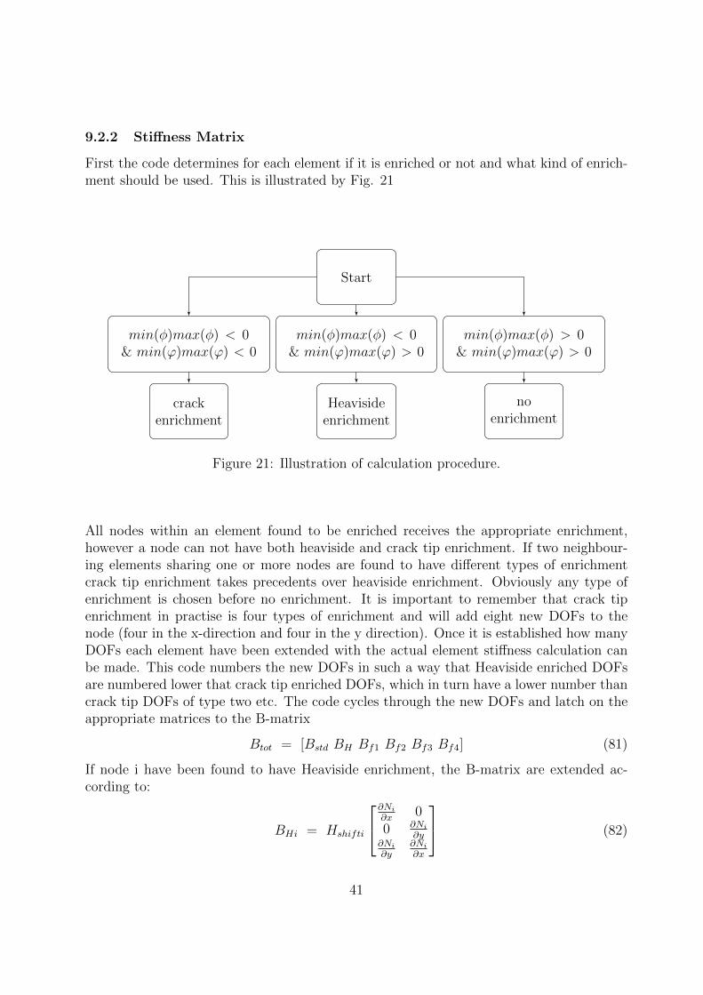
9.2.2 Stiffness Matrix
First the code determines for each element if it is enriched or not and what kind of enrich-ment should be used. This is illustrated by Fig. 21
Start
min(φ)max(φ) < 0& min(ϕ)max(ϕ) > 0
min(φ)max(φ) < 0& min(ϕ)max(ϕ) < 0
min(φ)max(φ) > 0& min(ϕ)max(ϕ) > 0
crackenrichment
Heavisideenrichment
noenrichment
Figure 21: Illustration of calculation procedure.
All nodes within an element found to be enriched receives the appropriate enrichment,however a node can not have both heaviside and crack tip enrichment. If two neighbour-ing elements sharing one or more nodes are found to have different types of enrichmentcrack tip enrichment takes precedents over heaviside enrichment. Obviously any type ofenrichment is chosen before no enrichment. It is important to remember that crack tipenrichment in practise is four types of enrichment and will add eight new DOFs to thenode (four in the x-direction and four in the y direction). Once it is established how manyDOFs each element have been extended with the actual element stiffness calculation canbe made. This code numbers the new DOFs in such a way that Heaviside enriched DOFsare numbered lower that crack tip enriched DOFs, which in turn have a lower number thancrack tip DOFs of type two etc. The code cycles through the new DOFs and latch on theappropriate matrices to the B-matrix
Btot = [Bstd BH Bf1 Bf2 Bf3 Bf4] (81)
If node i have been found to have Heaviside enrichment, the B-matrix are extended ac-cording to:
BHi = Hshifti
∂Ni
∂x0
0 ∂Ni
∂y∂Ni
∂y∂Ni
∂x
(82)
41

Note that ∂H∂x
= 0. Similarly in case node j needs crack tip extra DOFs the code extendsthe B-matrix as follows:
Bf1j =
∂Nj
∂xf1j + ∂f1j
∂xNj 0
0∂Nj
∂yf1j +
∂f1j∂yNj
∂Nj
∂yf1j + ∂f1j
∂yNj
∂Nj
∂xf1j + ∂f1j
∂xNj
(83)
The other three variants follow exactly the same pattern. There is however a nest of chainrule derivatives hidden within ∂f1j
∂xand ∂f1j
∂ythat could use some clarification. The B-matrix
requires the derivative of the enrichment function with respect to the global coordinates.The enrichment function is given in crack tip polar coordinates
∂f1
∂x=
∂f1
∂r
∂r
∂x+∂f1
∂θ
∂θ
∂x(84)
Crack tip polar coordinates are a function of Cartesian crack coordinates which in turn area rotation of the global coordinates with the crack angle ω. First it is noted that
∂r
∂x=
∂r
∂xrot
∂xrot∂x
+∂r
∂yrot
∂yrot∂x
(85)
∂θ
∂x=
∂θ
∂xrot
∂xrot∂x
+∂θ
∂yrot
∂yrot∂x
(86)
Recalling some useful relationships between the polar/Cartesian and rotated coordinatesystems:
xrot = r cos(θ) (87)
yrot = r sin(θ) (88)
xrot = x cos(ω) + y sin(ω) (89)
yrot = −x sin(ω) + y cos(ω) (90)
42
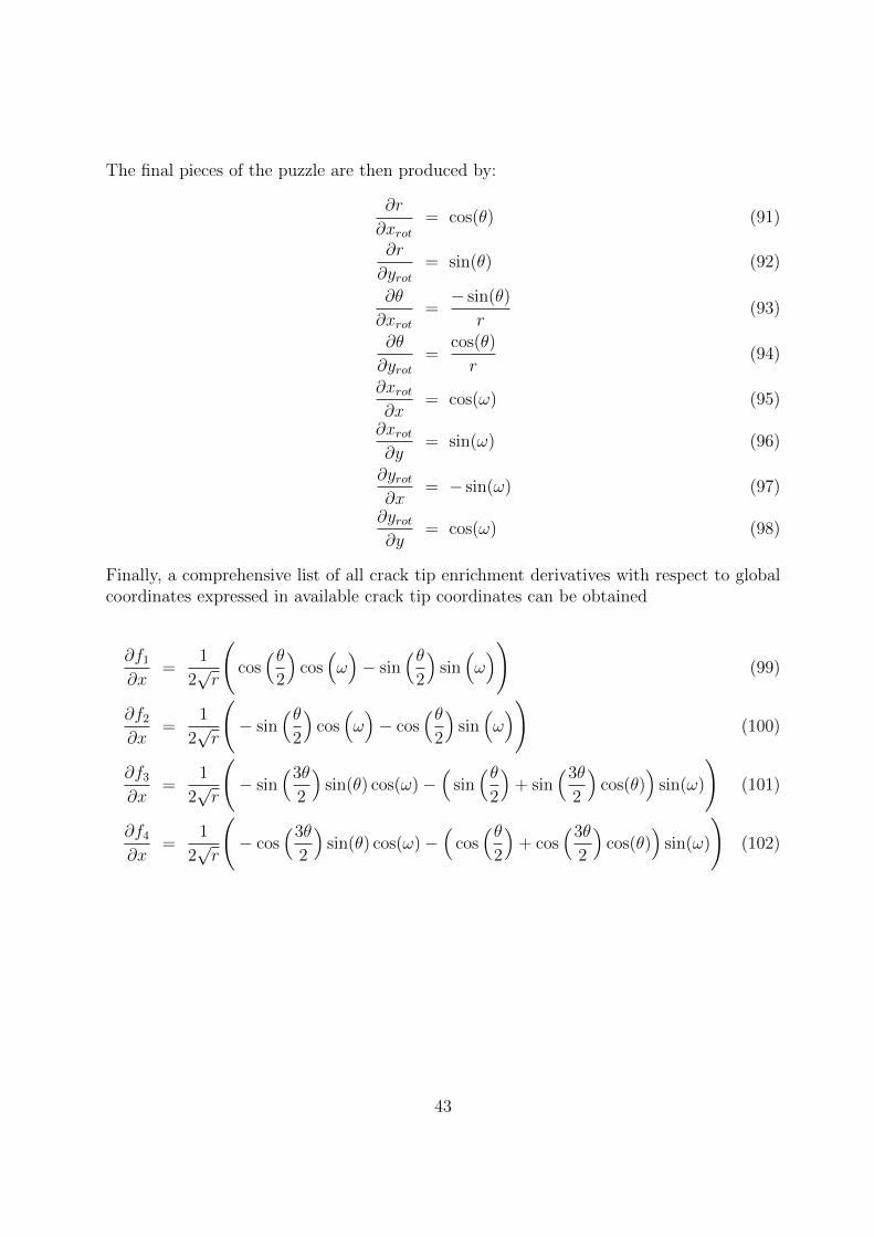
The final pieces of the puzzle are then produced by:
∂r
∂xrot= cos(θ) (91)
∂r
∂yrot= sin(θ) (92)
∂θ
∂xrot=− sin(θ)
r(93)
∂θ
∂yrot=
cos(θ)
r(94)
∂xrot∂x
= cos(ω) (95)
∂xrot∂y
= sin(ω) (96)
∂yrot∂x
= − sin(ω) (97)
∂yrot∂y
= cos(ω) (98)
Finally, a comprehensive list of all crack tip enrichment derivatives with respect to globalcoordinates expressed in available crack tip coordinates can be obtained
∂f1
∂x=
1
2√r
(cos(θ
2
)cos(ω)− sin
(θ2
)sin(ω))
(99)
∂f2
∂x=
1
2√r
(− sin
(θ2
)cos(ω)− cos
(θ2
)sin(ω))
(100)
∂f3
∂x=
1
2√r
(− sin
(3θ
2
)sin(θ) cos(ω)−
(sin(θ
2
)+ sin
(3θ
2
)cos(θ)
)sin(ω)
)(101)
∂f4
∂x=
1
2√r
(− cos
(3θ
2
)sin(θ) cos(ω)−
(cos(θ
2
)+ cos
(3θ
2
)cos(θ)
)sin(ω)
)(102)
43
∂f1
∂y=
1
2√r
(cos(θ
2
)sin(ω) + sin
(θ2
)cos(ω)
)(103)
∂f2
∂y=
1
2√r
(− sin
(θ2
)sin(ω) + cos
(θ2
)cos(ω)
)(104)
∂f3
∂y=
1
2√r
(− sin
(3θ
2
)sin(θ) sin(ω) +
(sin
(θ
2
)+ sin
(3θ
2
)cos(θ)
)cos(ω)
)(105)
∂f4
∂y=
1
2√r
(− cos
(3θ
2
)sin(θ) sin(ω) +
(cos
(θ
2
)+ cos
(3θ
2
)cos(θ)
)cos(ω)
)(106)
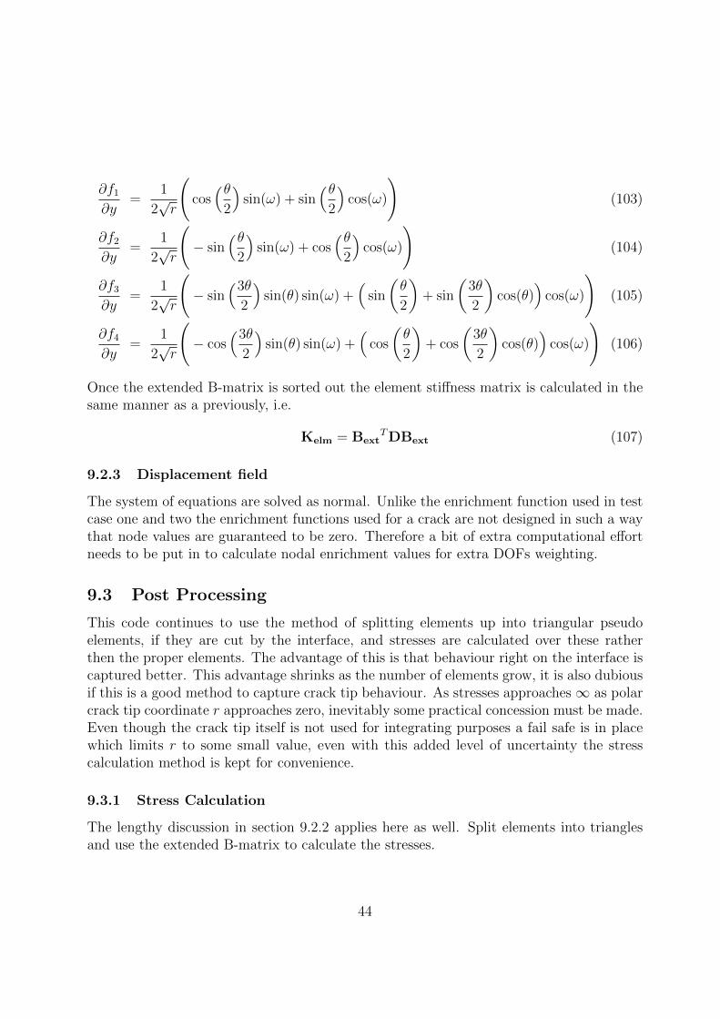
Once the extended B-matrix is sorted out the element stiffness matrix is calculated in thesame manner as a previously, i.e.
Kelm = BextTDBext (107)
9.2.3 Displacement field
The system of equations are solved as normal. Unlike the enrichment function used in testcase one and two the enrichment functions used for a crack are not designed in such a waythat node values are guaranteed to be zero. Therefore a bit of extra computational effortneeds to be put in to calculate nodal enrichment values for extra DOFs weighting.
9.3 Post Processing
This code continues to use the method of splitting elements up into triangular pseudoelements, if they are cut by the interface, and stresses are calculated over these ratherthen the proper elements. The advantage of this is that behaviour right on the interface iscaptured better. This advantage shrinks as the number of elements grow, it is also dubiousif this is a good method to capture crack tip behaviour. As stresses approaches∞ as polarcrack tip coordinate r approaches zero, inevitably some practical concession must be made.Even though the crack tip itself is not used for integrating purposes a fail safe is in placewhich limits r to some small value, even with this added level of uncertainty the stresscalculation method is kept for convenience.
9.3.1 Stress Calculation
The lengthy discussion in section 9.2.2 applies here as well. Split elements into trianglesand use the extended B-matrix to calculate the stresses.
44
9.3.2 Validation
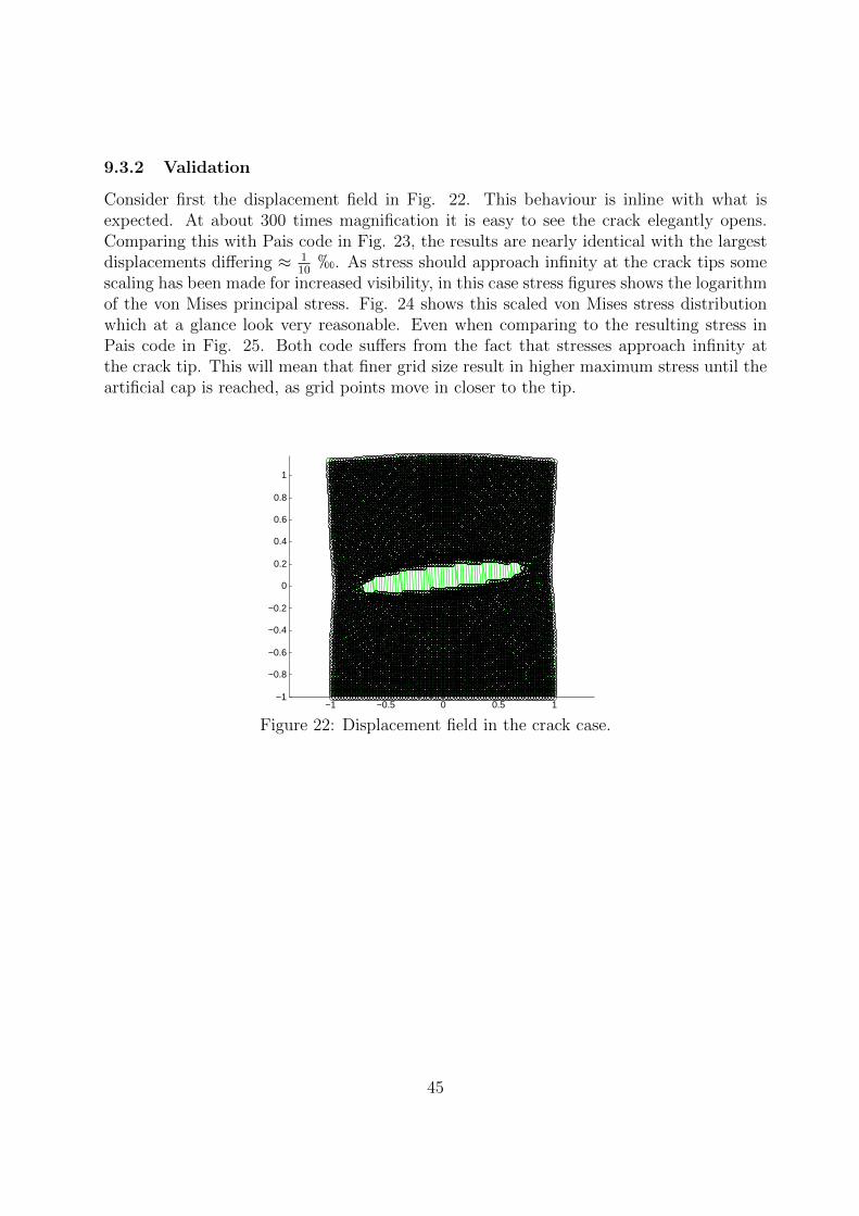
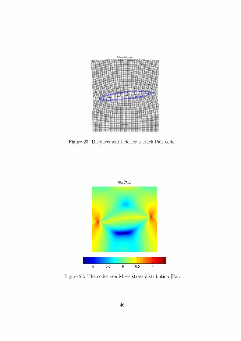
Consider first the displacement field in Fig. 22. This behaviour is inline with what isexpected. At about 300 times magnification it is easy to see the crack elegantly opens.Comparing this with Pais code in Fig. 23, the results are nearly identical with the largestdisplacements differing ≈ 1
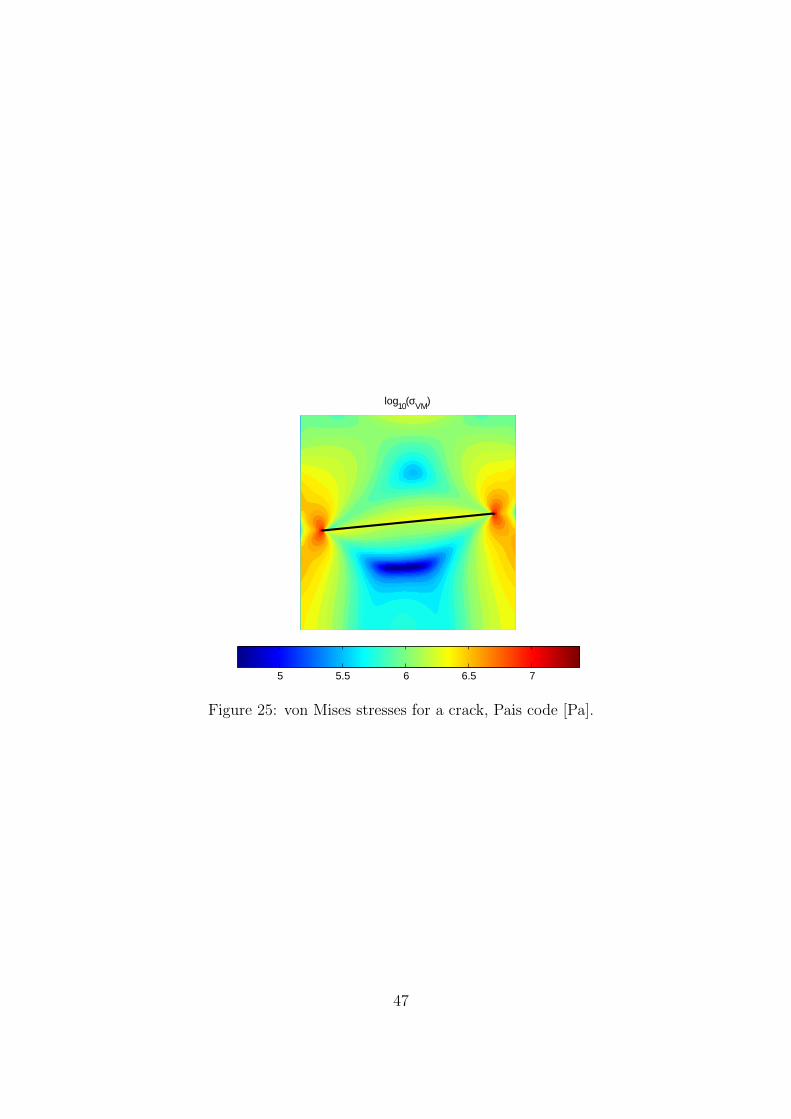
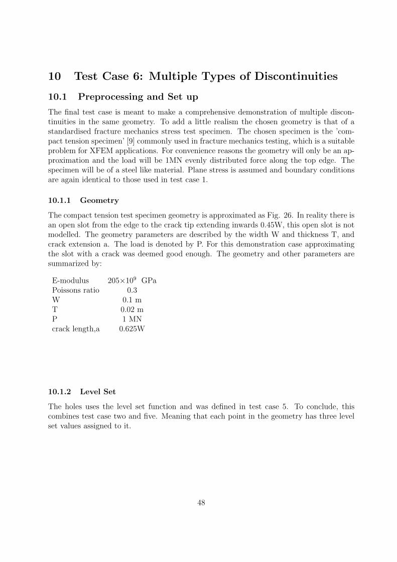
10h. As stress should approach infinity at the crack tips some
scaling has been made for increased visibility, in this case stress figures shows the logarithmof the von Mises principal stress. Fig. 24 shows this scaled von Mises stress distributionwhich at a glance look very reasonable. Even when comparing to the resulting stress inPais code in Fig. 25. Both code suffers from the fact that stresses approach infinity atthe crack tip. This will mean that finer grid size result in higher maximum stress until theartificial cap is reached, as grid points move in closer to the tip.
−1 −0.5 0 0.5 1−1
−0.8
−0.6
−0.4
−0.2
0
0.2
0.4
0.6
0.8
1
Figure 22: Displacement field in the crack case.
45
Deformed Geometry
Figure 23: Displacement field for a crack Pais code.
Figure 24: The codes von Mises stress distribution [Pa].
46
log10(σVM)
5 5.5 6 6.5 7
Figure 25: von Mises stresses for a crack, Pais code [Pa].
47
10 Test Case 6: Multiple Types of Discontinuities
10.1 Preprocessing and Set up
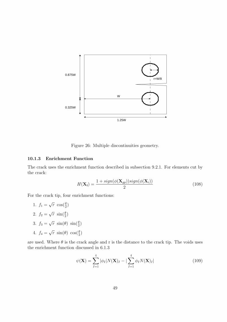
The final test case is meant to make a comprehensive demonstration of multiple discon-tinuities in the same geometry. To add a little realism the chosen geometry is that of astandardised fracture mechanics stress test specimen. The chosen specimen is the ’com-pact tension specimen’ [9] commonly used in fracture mechanics testing, which is a suitableproblem for XFEM applications. For convenience reasons the geometry will only be an ap-proximation and the load will be 1MN evenly distributed force along the top edge. Thespecimen will be of a steel like material. Plane stress is assumed and boundary conditionsare again identical to those used in test case 1.
10.1.1 Geometry
The compact tension test specimen geometry is approximated as Fig. 26. In reality there isan open slot from the edge to the crack tip extending inwards 0.45W, this open slot is notmodelled. The geometry parameters are described by the width W and thickness T, andcrack extension a. The load is denoted by P. For this demonstration case approximatingthe slot with a crack was deemed good enough. The geometry and other parameters aresummarized by:
E-modulus 205×109 GPaPoissons ratio 0.3W 0.1 mT 0.02 mP 1 MNcrack length,a 0.625W
10.1.2 Level Set
The holes uses the level set function and was defined in test case 5. To conclude, thiscombines test case two and five. Meaning that each point in the geometry has three levelset values assigned to it.
48
1.25W
W
0.325W
0.875Wr=W/8
Figure 26: Multiple discontinuities geometry.
10.1.3 Enrichment Function
The crack uses the enrichment function described in subsection 9.2.1. For elements cut bythe crack:
H(Xi) =1 + sign(φ(Xgp))sign(φ(Xi))
2(108)
For the crack tip, four enrichment functions:
1. f1 =√r cos( θ
2)
2. f2 =√r sin( θ
2)
3. f3 =√r sin(θ) sin( θ
2)
4. f4 =√r sin(θ) cos( θ
2)
are used. Where θ is the crack angle and r is the distance to the crack tip. The voids usesthe enrichment function discussed in 6.1.3
ψ(X) =4∑I=1
|φI |N(X)I − |4∑I=1
φIN(X)I | (109)
49
10.1.4 Stiffness Matrix
The stiffness matrix is extended like the other test cases but this time using all the (six)applied enrichment types void, crack and four types of crack tip enrichment. Lets numberthe possible B-matrices 1-7. B1 is the standard B-matrix. Enriched B-matrices (2-7) arecalculated according to:
BenrchJ I =
(ψJ(X)NI), x 00 (ψJ(X)NI), y
(ψJ(X)NI), y (ψJ(X)NI), x
(110)
Where each B matrix uses components from all four shape functions (I=1-4) and its ap-propriate enrichment function ψJ (J=2-7). Resulting in a total extended stiffness matrix
K11 K12 K13 K14 K15 K16 K17
K21 K22 K23 K24 K25 K26 K27
K31 K32 K33 K34 K35 K36 K37
K41 K42 K43 K44 K45 K46 K47
K51 K52 K53 K54 K55 K56 K57
K61 K62 K63 K64 K65 K66 K67
K71 K72 K73 K74 K75 K76 K77
(111)
10.1.5 Displacement field
As all other test cases, the only difference is that the stiffness matrix is larger, i.e. sym-bolically the solution is given as
K11 K12 K13 K14 K15 K16 K17
K21 K22 K23 K24 K25 K26 K27
K31 K32 K33 K34 K35 K36 K37
K41 K42 K43 K44 K45 K46 K47
K51 K52 K53 K54 K55 K56 K57
K61 K62 K63 K64 K65 K66 K67
K71 K72 K73 K74 K75 K76 K77
−1
F =
a1
a2
a3
a4
a5
a6
a7
(112)
10.2 Post Processing
Again as before, the enriched degrees of freedom are superimposed on top of the standarddofs which are used to calculate stresses.
50
10.2.1 Stress Calculation
Using all appropriate enrichments, the stress is calculated according to:
σ = D[
B1 ... B7
] u1
...u7
(113)
10.2.2 Validation
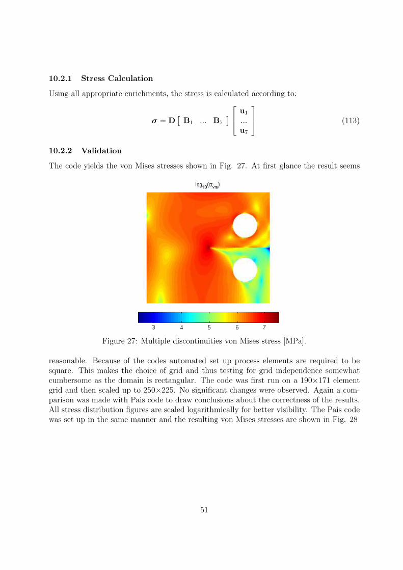
The code yields the von Mises stresses shown in Fig. 27. At first glance the result seems
Figure 27: Multiple discontinuities von Mises stress [MPa].
reasonable. Because of the codes automated set up process elements are required to besquare. This makes the choice of grid and thus testing for grid independence somewhatcumbersome as the domain is rectangular. The code was first run on a 190×171 elementgrid and then scaled up to 250×225. No significant changes were observed. Again a com-parison was made with Pais code to draw conclusions about the correctness of the results.All stress distribution figures are scaled logarithmically for better visibility. The Pais codewas set up in the same manner and the resulting von Mises stresses are shown in Fig. 28
51
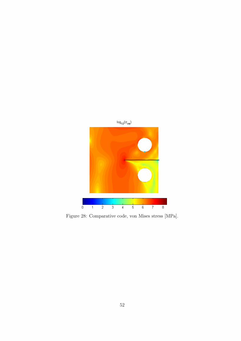
Figure 28: Comparative code, von Mises stress [MPa].
52
11 Conclusion and Summary
11.1 Level Sets
The level set method proved to be a convenient way to keep track of the discontinuity’splacement. As long as the interface is not set by a large number of vertices, which themethod described in section 3.4.3 would allow, very little computational effort needs tobe spent to obtain a mesh independent description of the geometrical shape of the discon-tinuity. Even though enrichment can be quite different, no particular difference betweenopen and closed discontinuities are found. All level sets discussed in this work are someform of a signed distance function which is both computationally inexpensive and easy toimplement.
In test case three (section 7) it was shown that an arbitrary discontinuity interface couldbe created by a set of vertices. The test case dealt with closed interfaces but there areno particular obstacles to overcome when using this method on open interfaces, somethingthat could be useful when simulating for example crack growth in directions not alignedwith the original crack. This method involves some approximation as connections betweenvertices are considered as straight lines. This assumption does however, in most cases, notcreate larger errors than the element partition used when calculating element stiffness usingfirst order shape functions. The method does however severely increase the computationaleffort needed as level set data needs to be calculated for each pair of neighbouring verticesbefore selecting the best fit rather than inserting coordinates into a fixed function.
When introducing moving boundaries some extra computational work will appear. Eachiteration step must have a sub step where relevant physical properties are calculated andcompared to some movement criteria. This should be mitigated by the mesh independentnature of the level set method meaning no remeshing will be needed, though a judgementcall for each type of problem is advised.
11.2 Enrichments
The enrichment functions addressed in this work were all relatively easy to implement whileproviding a solid method of obtaining the desired physical behaviour. All while being moreor less directly linked to the level set function(s). For example in the crack tip enrichmentcase, due to the duality of the tangential level set function, level set orientation is obscuredon an element level and help variables for distance to crack tip (r) and crack angle (θ)must be calculated. The enrichment function described in section 4.1.4 was proven veryuseful. Having the enrichment equal zero in element nodes saves a lot of computationaleffort and allows for some short cuts to be made. For crack tip enrichment the enrichmentfunctions were a bit more involved but as this type of enrichment can only be present in alow number of elements per simulation this extra expense is hardly noticeable.
53
11.3 Application
Some effort needs to be spent in post processing to display the results graphically. In theprogram accompanying this paper the element partitioning technique, used in element stiff-ness matrix calculation, is revisited for elements cut by the interface and each side of theinterface have its stresses averaged and graphed individually. The gain in computationaleffort XFEM provides is most obvious when simulations normally would require updatingthe mesh. An obvious example is crack growth simulation. Other potential favourable im-plementations could be in a design phase where several simulations over a single geometryare needed. Perhaps for finding optimum hole or inclusion placement, a single mesh couldbe used for all simulations. Another potential candidate is numerical calculations on com-posite materials. The different properties of such a material’s layers could be describedby the XFE-method. The program developed in conjunction to this work have severalweaknesses. It is not very efficient, it was consistently outperformed by the more opti-mized comparative program. Another weakness is the incapability of enriching an elementwith multiple types of enrichment. As the code determine a single type of enrichment andcalls a function for that type of element stiffness matrix. A better way would be to cycletrough all types of possible enrichment and ask ”is this present?” and assemble an elementB-matrix before calculating the element stiffness matrix.
11.4 Future Work
The most pressing feature to expand the code with is probably to introduce some crackgrowth possibility. A good start would be to introduce quasi static crack growth. Fracturemechanics parameters must be calculated and some criteria for crack growth and path areneeded. This has the potential to be further expanded to a dynamic simulation with cyclicload for use when fatigue fracture is of interest. The code could use some optimisationas it is not particularly efficient. The desired ”plug and play” feature of the ’SetUp’ and’XFEMmain’ files are possibly of limited use as it does not allow for much variation ingeometry, though the rest of the individual files could find use as extending an existinglibrary. Another improvement of the code could use is allowing for multiple types ofenrichment in the stiffness matrix assembly process.
54

Appendices
55
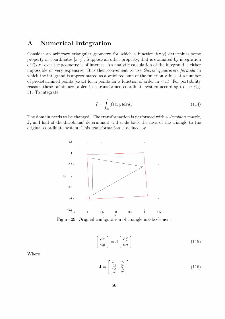
A Numerical Integration
Consider an arbitrary triangular geometry for which a function f(x,y) determines someproperty at coordinates [x; y]. Suppose an other property, that is evaluated by integrationof f(x,y) over the geometry is of interest. An analytic calculation of the integrand is eitherimpossible or very expensive. It is then convenient to use Gauss’ quadrature formula inwhich the integrand is approximated as a weighted sum of the function values at a numberof predetermined points (exact for n points for a function of order m < n). For portabilityreasons these points are tabled in a transformed coordinate system according to the Fig.31. To integrate
I =
∫4f(x, y)dxdy (114)
The domain needs to be changed. The transformation is performed with a Jacobian matrix,J, and half of the Jacobians’ determinant will scale back the area of the triangle to theoriginal coordinate system. This transformation is defined by
−1.5 −1 −0.5 0 0.5 1 1.5−1.5
−1
−0.5
0
0.5
1
1.5
x
y
Figure 29: Original configuration of triangle inside element
[dxdy
]= J
[dξdη
](115)
Where
J =
[∂x∂ξ
∂x∂η
∂y∂ξ
∂y∂η
](116)
56
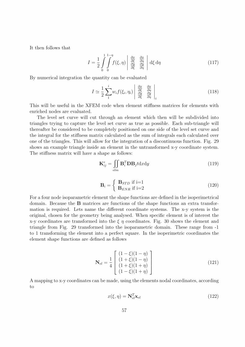
It then follows that
I =1
2
1∫0
1−η∫0
f(ξ, η)
∣∣∣∣∣ ∂x∂ξ
∂x∂η
∂y∂ξ
∂y∂η
∣∣∣∣∣ dξ dη (117)
By numerical integration the quantity can be evaluated
I ' 1
2
i∑1
wif(ξi, ηi)
∣∣∣∣∣ ∂x∂ξ
∂x∂η
∂y∂ξ
∂y∂η
∣∣∣∣∣i
(118)
This will be useful in the XFEM code when element stiffness matrices for elements withenriched nodes are evaluated.
The level set curve will cut through an element which then will be subdivided intotriangles trying to capture the level set curve as true as possible. Each sub-triangle willthereafter be considered to be completely positioned on one side of the level set curve andthe integral for the stiffness matrix calculated as the sum of integrals each calculated overone of the triangles. This will allow for the integration of a discontinuous function. Fig. 29shows an example triangle inside an element in the untransformed x-y coordinate system.The stiffness matrix will have a shape as follows:
Keij =
x
elm
BTi DBjtdxdy (119)
Bi =
BSTD if i=1BENR if i=2
(120)
For a four node isoparametric element the shape functions are defined in the isoperimetricaldomain. Because the B matrices are functions of the shape functions an extra transfor-mation is required. Lets name the different coordinate systems. The x-y system is theoriginal, chosen for the geometry being analysed. When specific element is of interest thex-y coordinates are transformed into the ξ η coordinates. Fig. 30 shows the element andtriangle from Fig. 29 transformed into the isoparametric domain. These range from -1to 1 transforming the element into a perfect square. In the isoperimetric coordinates theelement shape functions are defined as follows
Nel =1
4
(1− ξ)(1− η)(1 + ξ)(1− η)(1 + ξ)(1 + η)(1− ξ)(1 + η)
(121)
A mapping to x-y coordinates can be made, using the elements nodal coordinates, accordingto
x(ξ, η) = NTelxel (122)
57
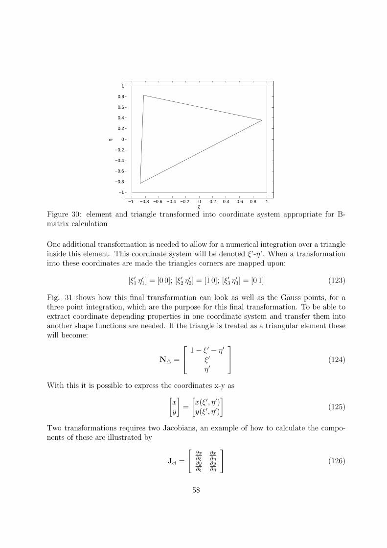
−1 −0.8 −0.6 −0.4 −0.2 0 0.2 0.4 0.6 0.8 1
−1
−0.8
−0.6
−0.4
−0.2
0
0.2
0.4
0.6
0.8
1
ξ
η
Figure 30: element and triangle transformed into coordinate system appropriate for B-matrix calculation
One additional transformation is needed to allow for a numerical integration over a triangleinside this element. This coordinate system will be denoted ξ’-η’. When a transformationinto these coordinates are made the triangles corners are mapped upon:
[ξ′1 η′1] = [0 0]; [ξ′2 η
′2] = [1 0]; [ξ′3 η
′3] = [0 1] (123)
Fig. 31 shows how this final transformation can look as well as the Gauss points, for athree point integration, which are the purpose for this final transformation. To be able toextract coordinate depending properties in one coordinate system and transfer them intoanother shape functions are needed. If the triangle is treated as a triangular element thesewill become:
N4 =
1− ξ′ − η′ξ′
η′
(124)
With this it is possible to express the coordinates x-y as[xy
]=
[x(ξ′, η′)y(ξ′, η′)
](125)
Two transformations requires two Jacobians, an example of how to calculate the compo-nents of these are illustrated by
Jel =
[∂x∂ξ
∂x∂η
∂y∂ξ
∂y∂η
](126)
58
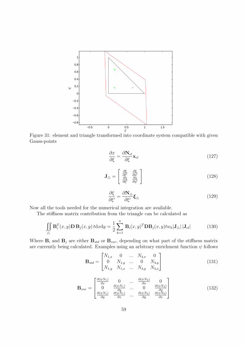
−0.5 0 0.5 1 1.5
−0.8
−0.6
−0.4
−0.2
0
0.2
0.4
0.6
0.8
1
ξ’
η’
Figure 31: element and triangle transformed into coordinate system compatible with givenGauss-points
∂x
∂ξ=∂Nel
∂ξxel (127)
J4 =
[∂ξ∂ξ′
∂ξ∂η′
∂η∂ξ′
∂η∂η′
](128)
∂ξ
∂ξ′=∂N4∂ξ′
ξ4 (129)
Now all the tools needed for the numerical integration are available.The stiffness matrix contribution from the triangle can be calculated as
x
4
BTi (x, y)D Bj(x, y) tdxdy =
1
2
n∑k=1
Bi(x, y)TDBj(x, y)twk|J4| |Jel| (130)
Where Bi and Bj are either Bstd or Benr, depending on what part of the stiffness matrixare currently being calculated. Examples using an arbitrary enrichment function ψ follows
Bstd =
N1,x 0 ... N4,x 00 N1,y ... 0 N4,y
N1,y N1,x ... N4,y N4,x
(131)
Benr =
∂(ψN1)∂x
0 ... ∂(ψN4)∂x
0
0 ∂(ψN1)∂y
... 0 ∂(ψN4)∂y
∂(ψN1)∂y
∂(ψN1)∂x
... ∂(ψN4)∂y
∂(ψN4)∂x
(132)
59
This is the target expression
N1,x =∂ξ
∂x
∂N1
∂ξ+∂η
∂x
∂N1
∂η(133)
For the enriched B-matrix
∂(ψN1)
∂x= N1
∂ψ
∂x+∂N1
∂xψ (134)
The enrichment function can be chosen to make the derivative trivial. The shape functionis given in isoperimetrical coordinates
∂N1
∂ξ= η − 1 (135)
The Jacobian can be used to access the derivatives of the shape functions w.r.t. x-ycoordinates [
∂N1
∂ξ∂N1
∂η
]= JT
[∂N1
∂x∂N1
∂y
](136)
Plug in the current gauss-point to extract the desired quantities[∂N1
∂x∂N1
∂y
]= J(ξgp, ηgp)
T−1
[ηgp − 1ξgp − 1
](137)
60

B Program Manual
B.1 Introduction
This collection of files are meant to be used for eXtended Finite Element (XFEM) cal-culations. They are written in a syntax compatible with Matlab. Some of the files arerequired to run in tandem with files from the finite element package CALFEM, developedby the division for solid mechanics at LTH Lunds University. The XFEM files can be usedindividually or together as a pre-built program according to the flowchart found at the endof this document.
61
B.2 crackLvlSet
B.2.1 Purpose
Calculates ψ and φ element level set values.
B.2.2 Syntax
[lvlsCrack] = crackLvlSet(ex, ey, start, stop)
B.2.3 Description
lvlscrack = [ψ1 ψ2 ψ3 ψ4 φ1 φ2 φ3 φ4]
ex and ey are element coordinates for the entire set of N elements
ex =
x11 x1
2 x13 x1
4...
xN1 xN2 xN3 xN4
ey =
y11 y1
2 y13 y1
4...
yN1 yN2 yN3 yN4
start and stop are coordinates for the first and second cracktip on the form [xct yct]
62
B.3 crackStiff
B.3.1 Purpose
Calculates element stiffness matrix with crack enrichments.
B.3.2 Syntax
[Kcrack] = crackStiff(ex, ey, lvlset, cracktipXY, edof, D, thickness)
B.3.3 Description
Identifies type of enrichment from edof, partitions the element defined by ex and ey ac-cording to the lvlset vector, and calculates the element stiffness matrix;
ex = [x1 x2 x3 x4]
ey = [y1 y2 y3 y4]
(138)
lvlset(1 : 12) = [not crack related]
lvlset(13 : 16) = [ψ1 ψ2 ψ3 ψ4]
lvlset(17 : 20) = [φ1 φ2 φ3 φ4]
Corner level set values orthogonally/perpendicular (ψ/φ)to the crack edof(1:32) is reservedfor other degrees of freedom.Crack enrichment:
edof(34 : 41) = [Cdof1 Cdof2 ... Cdof8]
63

Crack tip enrichment (4 types):
edof(42 : 49) = [CTdof 11 CTdof
12 ... CTdof
18 ]
edof(50 : 57) = [Ctdof 21 ... CTdof
28 ]
edof(58 : 65) = [CTdof 31 ... CTdofs
38]
edof(66 : 73) = [CTdofs41 ... CTdofs
48]
D is the constitutive matrix thickness is plate thickness cracktipXY is coordinates forboth cracktips in the format [
xct1 yct1xct2 yct2
]
64
B.4 crackStress
B.4.1 Purpose
Calculates element stresses from the displacements for an crack enriched element.
B.4.2 Syntax
[esx esy esxy] = crackStress(aEl, ex, ey, edof, lvlset, D, cracktipXY )
B.4.3 Description
Given element displacement (aEl), including those from enriched dofs, will calculate the di-agonal values in the element stress matrix using the element corners as integration points.ex and ey are element coordinate vectors. edof is a list of dofs for the element, infor-mation relevant for cracks are kept in edof(34:72). lvlset are element corner level setvalues, lvlset(13:16)=[ψ1 ... ψ4], lvlset(17:20)=[φ1 ... φ4]. D is the constitutive matrix andcracktipXY=[CT1x CT1y; CT2x CT2y].
65
B.5 cutK
B.5.1 Purpose
Calculating the element stiffness matrix for an element on an interface.
B.5.2 Syntax
[Kuu Kua Kaa] = cutK(elx, ely, trix, triy, npnts, Dplus, Dminus, nodlvl)
B.5.3 Description
elx and ely are the element coordinates. trix and triy are coordinates for triangles, insidethe element where each triangle has two points with the same sign on its level set value, xand y respectively one row for each triangle. npnts are the number of gauss points desiredand nodlvl is the element level set values. Dplus and Dminus are the constitutive matricesfor the positive and negative valued sides of boundary with respect to the level set value.
66
B.6 definelvlSet
B.6.1 Purpose
To calculate element level set data.
B.6.2 Syntax
[lvlSet edof ] = definelvlSet(discs, ex, ey, edof)
B.6.3 Description
Input variable discs is a set up variable describing the number and types of discontinuities.One row for each discontinuity. First number in the row is the type of discontinuity.
type=1 - inclusionif circular:discs=[1 centre-xcoord centre-ycoord radius incl.E-modulus incl.pois-ratio]if polygonal (user defined vertices)discs=[1 vert1-x vert1-y vert2-x vert2-y ... vertn-x vertn-y incl.E-mod incl.pois-rat]type=2 - voidif circular:discs=[2 centre-x centre-y radius]polygonal:discs=[2 vert1-x vert1-y ... vertn-x vertn-y]type=3 - bimaterial domain, line shaped interfaceyou need to supply two points on this line (POL1 POL2), endpoints not required. SuppliedE-modulus and poissons ratio are for the side of the interface with negative level set values.discs=[3 POL1x POL1y POL2x POL2y E-mod poissons-ratio]discs=4 - crackTwo points in the domain that are the crack tips (CT1 CT2)discs=[4 CT1-x CT1-y CT2-x CT2-y]
ex and ey are element coordinate matrices and edof is element dofs for a standard FEMcase. Return variable lvlset is the element level set values distributed as follows:lvlset(n,:)=level set values for element n.lvlset(n,1:4)=ζ level set values for inclusions.lvlset(n,5:8)=ζ level set values for voids.
67
lvlset(n,9:12)=ψ level set values for a bimaterial interface.lvlset(n,13:16)=ψ level set values for cracks.lvlset(n,17:20)=φ level set values for cracks
Returning edof is the standard edof expanded with the appropriate XFEM dofs. edofis expanded like so:edof(n,10:17) - inclusion dofs for element nedof(n,18:25) - void dofsedof(n,26:33) - bimaterial dofedof(n,34:41) - crack dofsedof(n,42:49) - cracktip enrichment type 1 dofsedof(n,50:57) - cracktip enrichment 2 dofsedof(n,58:65) - cracktip enrichment 3 dofsedof(n,66:73) - cracktip enrichment 4 dofs
68
B.7 findXDOF
B.7.1 Purpose
Calculate extra dofs for extension of a element degrees of freedom list for a closed bound-ary. (used inside defineLvlSet to extend edof)
B.7.2 Syntax
[edofx] = findXDOF (edof, nrdof, nodlvl)
B.7.3 Description
edof is the standard edof matrix suitable for CALFEM.nrdof is the highest numbered degree of freedom in the standard edof.nodlvl is the element level set values.
69
B.8 polyLvlSet
B.8.1 Purpose
Calculates ζ level set values for a closed boundary defined by a series of vertices. (Thisfunction is called within definelvlSet).
B.8.2 Syntax
[polyLvlSet] = polyLvlset(verts, ex, ey)
B.8.3 Description
polyLvlSet(n,:)=[ζ1 ζ2 ζ3 ζ4], for element # nThe code approximates the boundary as the straight line between two neighbouring ver-tices. Therefore tighter placement of vertices gives better results.
70
B.9 remap
B.9.1 Purpose
Equation solver for backwards element mapping, global coordinates -> isoparametric ele-ment coordinates. Convenient when doing numeric integration for an element split up intotriangles and element coordinates for triangle corners (which are given in global coordi-nates) are needed.
B.9.2 Syntax
[xi eta] = remap(ex, ey, x, y)
B.9.3 Description
ey and ex are the element coordinates (y and x respectively).x and y are the user wants translated into element coordinates.The returned xi and eta are the element coordinates ξ & η.
71

B.10 trisplit
B.10.1 Purpose
Splits an element into triangles with uniform level set values.
B.10.2 Syntax
[tx ty] = trisplit(ex, ey, lvlSet);
B.10.3 Description
If the element is cut by the interface boundary described by the element level set valuessupplied by lvlset this function will split the element, defined by the element coordinatearrays ex and ey, into triangles where every point on each triangle have the same sign onits level set value.
72

B.11 weightedCrackDispl
B.11.1 Purpose
Superimposes XFEM crack dofs displacement with correct weight factor on correspondingstandard FE dofs.
B.11.2 Syntax
[atot] = weightedCrackDispl(a, edof, lvlset, ex, ey, CT )
B.11.3 Description
a are entire XFEM system resulting displacements, no weights applied.edof are the list of element degrees of freedom.ex and ey are lists of element coordinates, x and y respectivley.CT are cracktip coordinates, [CT1x CT1y; CT2x CT2y].
73
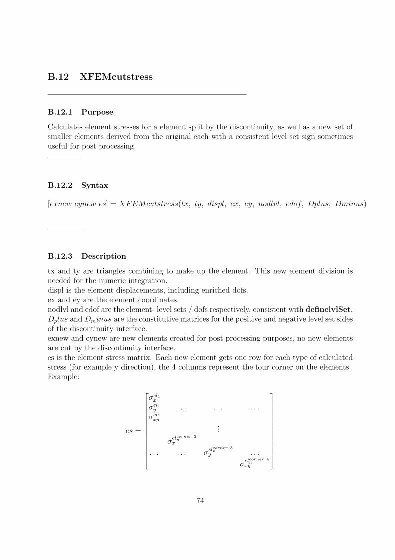
B.12 XFEMcutstress
B.12.1 Purpose
Calculates element stresses for a element split by the discontinuity, as well as a new set ofsmaller elements derived from the original each with a consistent level set sign sometimesuseful for post processing.
B.12.2 Syntax
[exnew eynew es] = XFEMcutstress(tx, ty, displ, ex, ey, nodlvl, edof, Dplus, Dminus)
B.12.3 Description
tx and ty are triangles combining to make up the element. This new element division isneeded for the numeric integration.displ is the element displacements, including enriched dofs.ex and ey are the element coordinates.nodlvl and edof are the element- level sets / dofs respectively, consistent with definelvlSet.Dplus and Dminus are the constitutive matrices for the positive and negative level set sidesof the discontinuity interface.exnew and eynew are new elements created for post processing purposes, no new elementsare cut by the discontinuity interface.es is the element stress matrix. Each new element gets one row for each type of calculatedstress (for example y direction), the 4 columns represent the four corner on the elements.Example:
es =
σel1xσel1y . . . . . . . . .σel1xy
...
σelcorner 2
nx
. . . . . . σelcorner 3
ny . . .
σelcorner 4
nxy
74
B.13 XFEMelstress
B.13.1 Purpose
Calculates element stresses for a enriched element, not cut by the ζ set = 0 interface.
B.13.2 Syntax
[es] = XFEMelstress(displ, ex, ey, nodlvl, edof, Dplus, Dminus)
B.13.3 Description
ex and ey are the element coordinate vectors.edof is the element dofs vector, including enriched ones following the convention fromdefinelevelSet.displ are the relevant displacements, including those from enriched nodes.nodlvl are the element level set values, also following definelvlSet conventions.Dplus and Dminus are the constitutive matrices for the positive and negative level set siderespectively.Returns element corner stresses es, one column per element corner one row per type ofstress:es(:,1) - stresses for corner 1 (southwest). etc.
75
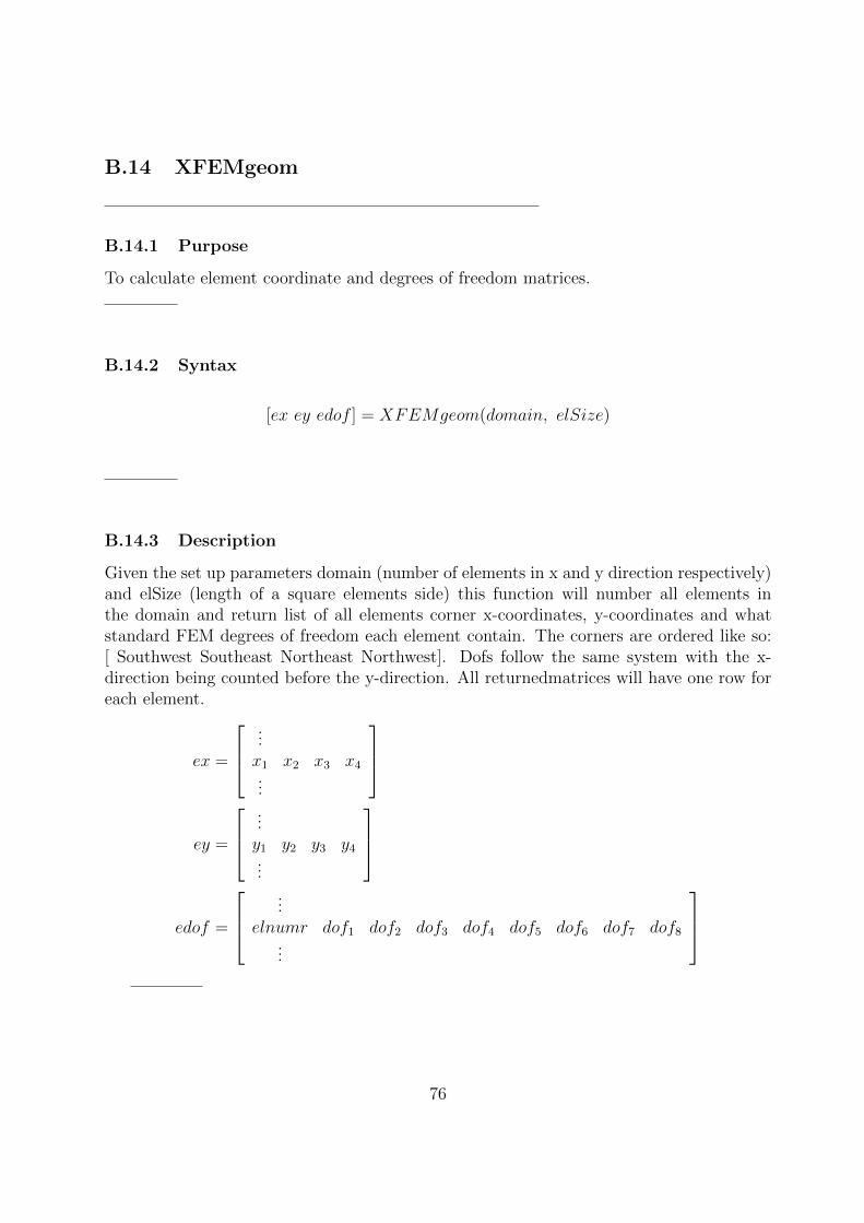
B.14 XFEMgeom
B.14.1 Purpose
To calculate element coordinate and degrees of freedom matrices.
B.14.2 Syntax
[ex ey edof ] = XFEMgeom(domain, elSize)
B.14.3 Description
Given the set up parameters domain (number of elements in x and y direction respectively)and elSize (length of a square elements side) this function will number all elements inthe domain and return list of all elements corner x-coordinates, y-coordinates and whatstandard FEM degrees of freedom each element contain. The corners are ordered like so:[ Southwest Southeast Northeast Northwest]. Dofs follow the same system with the x-direction being counted before the y-direction. All returnedmatrices will have one row foreach element.
ex =
...x1 x2 x3 x4...
ey =
...y1 y2 y3 y4...
edof =
...
elnumr dof1 dof2 dof3 dof4 dof5 dof6 dof7 dof8...
76
B.15 XFEMload
B.15.1 Purpose
Creates the load and boundary condition vectors.
B.15.2 Syntax
[f bc] = XFEMload(F, BC, edof, domain, lvlSet)
B.15.3 Description
F(1) is the location of the load on the rectangular domain1 - west2 - south3 - east4 - northF(2) is the total magnitude of the load.BC is the location where the domain is locked in place, follows the same convention as F(1)edof is the element degrees of freedom and lvlset is the element level set values, used incase enriched elements also are loaded/have locked dofs.domain(1) - number of elements in vertical direction.domain(2) - number of elements in horizontal direction.
77
B.16 XFEMplot
B.16.1 Purpose
Automated post processing.
B.16.2 Syntax
[ex2 ey2 es] = XFEMplot(a, ex, ey, edof, lvlSet, plots, Discs, parameters)
B.16.3 Description
a- total system displacements, including those from enriched dofs.ex and ey - element coordinates.edof - element dofs, including enriched dofs as described in definelvlSet.lvlset - element level set values.plots - series of integers each symbolising a type of figure the user wants ploted:1 - undeformed geometry, including boundary illustration.2 - deformed geometry, auto scaled for visibility.3 - Stresses in x direction.4 - Stresses in y direction.5 - Shear Stresses6 - Von Mises stresses.Discs and parameters are discontinuity and domain data as used in SetUp.This function calls an appropriate sub-function to calculate stresses before ploting, returnsthese as es for further processing.ex2 and ey2 are new element coordinates. The function creates these, when appropriate,to ensure elements with uniform level set value signs. Sometimes useful for calculatingstresses.
78
B.17 XFEMstiffness
B.17.1 Purpose
Returns a combined stiffness matrix, appropriate to what types of discontinuities arepresent.
B.17.2 Syntax
K = XFEMstiffness(ex, ey, Discs, lvlSet, edof, parameters)
B.17.3 Description
Using the level set values in lvlset to determine what type of discontinuity (or lack thereof)an element have. Calls the appropriate subfunction and using the element degrees offreedom list edof to insert the subfunction supplied element stiffness matrix in the correctplace in the system stiffness matrixex and ey are element coordinatematrices. Discs and parameters are set up variablesdiscussed in more detail in the description for the file SetUp.
79
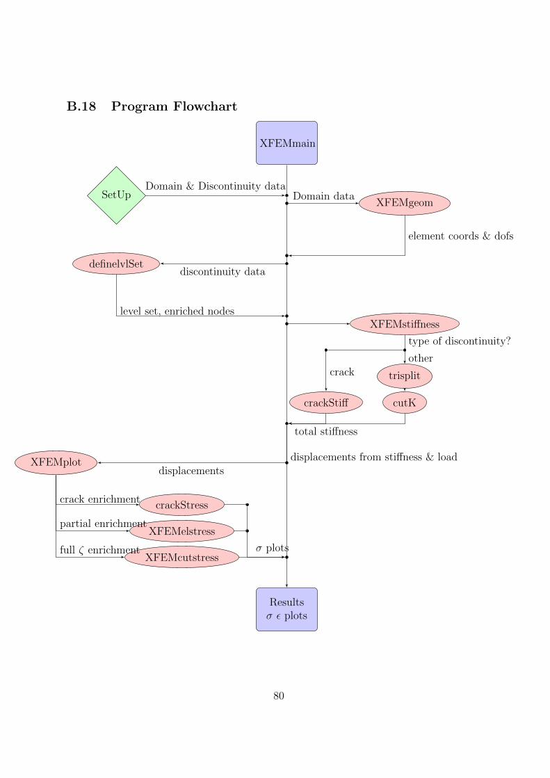
B.18 Program Flowchart
XFEMmain
Resultsσ ε plots
SetUpXFEMgeom
definelvlSet
XFEMstiffness
trisplit
cutKcrackStiff
XFEMplot
XFEMcutstress
XFEMelstress
crackStress
Domain & Discontinuity dataDomain data
element coords & dofs
discontinuity data
level set, enriched nodes
type of discontinuity?
othercrack
total stiffness
displacements
σ plots
crack enrichment
partial enrichment
full ζ enrichment
displacements from stiffness & load
80
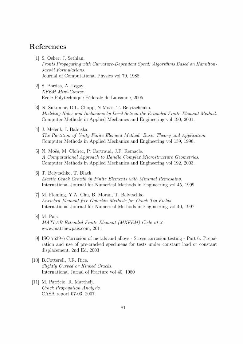
References
[1] S. Osher, J. Sethian.Fronts Propagating with Curvature-Dependent Speed: Algorithms Based on Hamilton-Jacobi Formulations.Journal of Computational Physics vol 79, 1988.
[2] S. Bordas, A. Legay.XFEM Mini-Course.Ecole Polytechnique Federale de Lausanne, 2005.
[3] N. Sukumar, D.L. Chopp, N Moes, T. Belytschenko.Modeling Holes and Inclusions by Level Sets in the Extended Finite-Element Method.Computer Methods in Applied Mechanics and Engineering vol 190, 2001.
[4] J. Melenk, I. Babuska.The Partition of Unity Finite Element Method: Basic Theory and Application.Computer Methods in Applied Mechanics and Engineering vol 139, 1996.
[5] N. Moes, M. Cloirec, P. Cartraud, J.F. Remacle.A Computational Approach to Handle Complex Microstructure Geometries.Computer Methods in Applied Mechanics and Engineering vol 192, 2003.
[6] T. Belytschko, T. Black.Elastic Crack Growth in Finite Elements with Minimal Remeshing.International Journal for Numerical Methods in Engineering vol 45, 1999
[7] M. Fleming, Y.A. Chu, B. Moran, T. Belytschko.Enriched Element-free Galerkin Methods for Crack Tip Fields.International Journal for Numerical Methods in Engineering vol 40, 1997
[8] M. Pais.MATLAB Extended Finite Element (MXFEM) Code v1.3.www.matthewpais.com, 2011
[9] ISO 7539-6 Corrosion of metals and alloys - Stress corrosion testing - Part 6: Prepa-ration and use of pre-cracked specimens for tests under constant load or constantdisplacement. 2nd Ed. 2003
[10] B.Cotterell, J.R. Rice.Slightly Curved or Kinked Cracks.International Jurnal of Fracture vol 40, 1980
[11] M. Patricio, R. Mattheij.Crack Propagation Analysis.CASA report 07-03, 2007.
81

[12] A. Carpinteri, L.P. Pook, L. Susmel, S. Vantadori.Foreward: Fatigue Crack Paths 2012 (CP 2012)International Journal of Fatigue, vol 58, 2014
82
![A hybrid XFEM - Phase Field (Xfield) method for crack … · 2016. 11. 10. · A hybrid XFEM - Phase Field (Xfield) method for crack propagation in brittle materials BIANCA GIOVANARDI],](https://img.pdfslide.us/doc/110x75/614a978a12c9616cbc69840e/a-hybrid-xfem-phase-field-xfield-method-for-crack-2016-11-10-a-hybrid-xfem.jpg)


![An XFEM method for modeling geometrically elaborate crack ... · AN XFEM METHOD FOR GEOMETRICALLY ELABORATE CRACK PROPAGATION 3 for holes and inclusions see [24]) and has also been](https://img.pdfslide.us/doc/110x75/5ad9bedd7f8b9a53618bac1b/an-xfem-method-for-modeling-geometrically-elaborate-crack-xfem-method-for-geometrically.jpg)
![A hybrid XFEM - Phase Field (Xfield) method for crack ... · A hybrid XFEM - Phase Field (Xfield) method for crack propagation in brittle materials BIANCA GIOVANARDI], ANNA SCOTTI](https://img.pdfslide.us/doc/110x75/5ade1d027f8b9a595f8db44e/a-hybrid-xfem-phase-field-xfield-method-for-crack-hybrid-xfem-phase-field.jpg)