Embed Size (px)
Citation preview

The eXtended Finite Element Method (XFEM) forbrittle and cohesive fracture
Prof. Dr. Eleni ChatziDr. Giuseppe Abbiati, Dr. Konstantinos Agathos
Lecture 7 - 16 November, 2017
Institute of Structural Engineering, ETH Zurich
November 16, 2017
Institute of Structural Engineering Method of Finite Elements II 1

Outline1 Introduction2 Discontinuities-High gradients3 Discretization methods4 Partition of unity enrichment5 Extended Finite Element Method for brittle fracture
Representation of discontinuitiesEnrichment functionsShape functions and derivativesStiffness matrixNumerical integrationEnrichment shiftingStress intensity factorsSolution overview
6 XFEM for cohesive fracture7 Extension to 3D
Institute of Structural Engineering Method of Finite Elements II 2

Learning goals
Introducing partition of unity enrichment
Introducing the eXtended/Generalized Finite Element Method(XFEM/GFEM)
Reviewing some implementation isuues
Application of XFEM in brittle fracture
Application of XFEM in cohesive fracture
Institute of Structural Engineering Method of Finite Elements II 3

Applications
Fracture in brittle materials
Fatigue fracture
Fracture in concrete
Institute of Structural Engineering Method of Finite Elements II 4

Discontinuities-High gradients
The methods presented are of interest for problems involvingdiscontinuities and high gradients
Those usually occur in the vicinity of, or along points, lines andinterfaces
The nature of these phenomena is therefore mostly local
Often those interfaces evolve over time
Representation of moving interfaces may become an importantissue
Institute of Structural Engineering Method of Finite Elements II 5

Strong discontinuitiesStrong discontinuities:
Discontinuities in the main solution variable
Example: Displacement jump along crack faces
crack
Displacement
Strain
Institute of Structural Engineering Method of Finite Elements II 6

Weak discontinuitiesWeak discontinuities:
Discontinuities in the derivatives of the main solution variable
Example: Strain discontinuity in bi-material interfaces
bimaterial interface
Displacement
Strain
material 1
material 2
Institute of Structural Engineering Method of Finite Elements II 7

High gradients
High gradients:
Large variation of a variable in a small area
Example: Strain singularity around the tip of a crack
Institute of Structural Engineering Method of Finite Elements II 8

Standard FEMFEM solution of a problem involving discontinuities and singularitiesalong moving interfaces (e.g. crack propagation):
Domain
Institute of Structural Engineering Method of Finite Elements II 9

Standard FEMFEM solution of a problem involving discontinuities and singularitiesalong moving interfaces (e.g. crack propagation):
Initial mesh
Institute of Structural Engineering Method of Finite Elements II 9

Standard FEMFEM solution of a problem involving discontinuities and singularitiesalong moving interfaces (e.g. crack propagation):
Crack appears → Re-meshing and mesh refinement is required
Institute of Structural Engineering Method of Finite Elements II 9

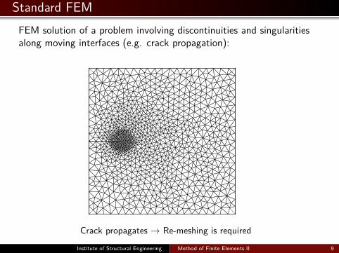
Standard FEMFEM solution of a problem involving discontinuities and singularitiesalong moving interfaces (e.g. crack propagation):
Crack propagates → Re-meshing is required
Institute of Structural Engineering Method of Finite Elements II 9
Standard FEMFEM solution of a problem involving discontinuities and singularitiesalong moving interfaces (e.g. crack propagation):
Crack propagates → Re-meshing is required
Institute of Structural Engineering Method of Finite Elements II 9

Standard FEMFEM solution of a problem involving discontinuities and singularitiesalong moving interfaces (e.g. crack propagation):
Crack propagates → Re-meshing is required
Institute of Structural Engineering Method of Finite Elements II 9

Standard FEMFEM solution of a problem involving discontinuities and singularitiesalong moving interfaces (e.g. crack propagation):
Crack propagates → Re-meshing is required
Institute of Structural Engineering Method of Finite Elements II 9

Standard FEM
Difficulties in the above approach:
In every step of crack propagation re-meshing is required
The procedure cannot be fully automated since the generatedmeshes need to be inspected
For nonlinear problems projection of solution parameters isrequired between meshes
Institute of Structural Engineering Method of Finite Elements II 10

Numerical solution of PDESBasic ingredients of numerical methods for PDEs:
Problem formulation:
Weak form, e.g.: Principle of Virtual Work, Galerkin Method,Hu-Washizu principle
Strong form
Discretization scheme, e.g.:
Piecewise polynomials
Splines
Radial basis functions
Institute of Structural Engineering Method of Finite Elements II 11

Numerical solution of PDES
By employing combinations of the above, different methods can beobtained, e.g.:
Weak form + Piecewise polynomials → FEM
The methods presented in the following mainly employ improveddiscretization schemes based on the standard FEM
Institute of Structural Engineering Method of Finite Elements II 12

Partition of unity
DefinitionA set of functions N∗I (x) defined in a domain Ω such that:∑
∀IN∗I (x) = 1, ∀I ∈ Ω
Is called a partition of unity (PU).
Example: FE shape functions
Institute of Structural Engineering Method of Finite Elements II 13

Partition of unity
Any function Ψ (x) can be exactly represented in Ω by theproduct: ∑
∀IN∗I (x) Ψ (x)
If the additional parameters bI are introduced, then the functioncan be spatially adjusted:∑
∀IN∗I (x) Ψ (x) bI
Institute of Structural Engineering Method of Finite Elements II 14

PU FEM
If a FE mesh is considered then the PU property can be exploited toenrich the approximation:
u (x) =∑∀I
NI (x) uI︸ ︷︷ ︸FE approximation
+∑∀I
N∗I (x) Ψ (x) bI︸ ︷︷ ︸enriched part
where:
u (x) The main solution variable (e.g. displacements)NI (x) The FE shape functions
uI Nodal dofsN∗I (x) A set of functions forming a PUΨ (x) The enrichment function
bI Additional unknowns
Institute of Structural Engineering Method of Finite Elements II 15

PU FEM
The above, for N∗I ≡ NI , becomes the Partition of Unity FiniteElement Method (PU FEM):
u (x) =∑∀I
NI (x) uI︸ ︷︷ ︸FE approximation
+∑∀I
NI (x) Ψ (x) bI︸ ︷︷ ︸enriched part
PU FEM allows for:
Incorporating known features of the problem in the solutionthrough Ψ (x)Spatially adjusting Ψ (x) to the specific problem solved throughbI
Preserving some desired properties of the FE method such assparsity of the system matrices
Institute of Structural Engineering Method of Finite Elements II 16

XFEM
Enrichment in PU FEM is global, i.e. it is applied to all nodesof the mesh
Phenomena such as cracks, holes and discontinuities are of localnature
The eXtended Finite Element Method (XFEM) was introducedto model discontinuities independently of the FE mesh used
The XFEM employs local enrichment, i.e. enrichment appliedonly to nodes in the vicinity of the discontinuity
Institute of Structural Engineering Method of Finite Elements II 17

Representation of discontinuities
In XFEM:
Discontinuities are not part of the mesh
The geometrical representation of evolving surfaces assumes animportant role
The Level Set Method (LSM) has been established as animportant tool for tracking discontinuities
Institute of Structural Engineering Method of Finite Elements II 18

Level Set Method
We consider a domain Ω divided in subdomains Ω1 and Ω2 by aninterface Γ, then:
→ Γ can be implicitly definedby a level set function φ (x)such that:
φ (x) > 0 in Ω1
φ (x) < 0 in Ω2
φ (x) = 0 on Γ
Institute of Structural Engineering Method of Finite Elements II 19

Level Set Method
Typically the signed distance function is used as a level set function:
φ (x) = minx∈Γ‖x− x‖ sign (n · (x− x))
where n is the normal vector to the interface and sign is the signfunction:
sign (x) =
1 for x > 0− 1 for x < 0
Signed distance functions have the property:
‖∇φ‖ = 1
Institute of Structural Engineering Method of Finite Elements II 20
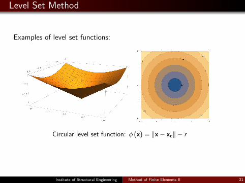
Level Set Method
Examples of level set functions:
Circular level set function: φ (x) = ‖x− xc‖ − r
Institute of Structural Engineering Method of Finite Elements II 21

Level Set Method
Examples of level set functions:
Elliptical level set function: φ (x , y) =(x
a
)2+(y
b
)2− 1
Institute of Structural Engineering Method of Finite Elements II 21

Level Set Method
Typically, level set values are computed for a set of points, e.g.all nodal points in an FE mesh
In many cases the initial LS function is not a signed distancefunction, e.g. for the elliptical LS:
φ (x , y) =(x
a
)2+(y
b
)2− 1
Then a Jacobi-Hamilton type equation is employed to imposethe condition ‖∇φ‖ = 1:
∂φ
∂τ+ sign (φ) (‖∇φ‖ − 1) = 0
Institute of Structural Engineering Method of Finite Elements II 22
Level Set Method
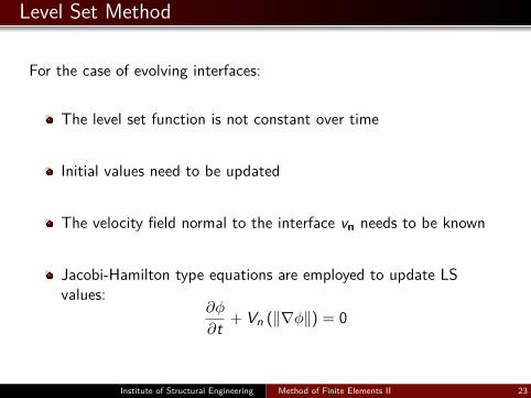
For the case of evolving interfaces:
The level set function is not constant over time
Initial values need to be updated
The velocity field normal to the interface vn needs to be known
Jacobi-Hamilton type equations are employed to update LSvalues:
∂φ
∂t + Vn (‖∇φ‖) = 0
Institute of Structural Engineering Method of Finite Elements II 23

Crack representation
To represent crack surfaces two LS functions are needed:
φ→ the signed distancefrom the crack surface
ψ → the signeddistance from thenormal to the cracksurface crack surface crack extension
) = 0x(ψ
)x(ψ
)x(φ
x
r
θ
) = 0x(φ
+n
crack front
Institute of Structural Engineering Method of Finite Elements II 24

Crack representation
The following relations should hold for the LS description of thecrack:
φ = 0 should give the crack surface
ψ = 0 should give the normal crack surface
φ = 0, ψ = 0 should give the crack front/ crack tip
‖∇φ‖ = 1, ‖∇ψ‖ = 1
∇φ · ∇ψ = 0
Institute of Structural Engineering Method of Finite Elements II 25

Propagating cracks
The propagation criterion is only evaluated at the cracktip/front
The velocity field is only known at those locations
To update the LS representation of the crack the velocity fieldneeds to be extended to the whole domain
Along with the previous conditions, an additional one needs tobe imposed such that the existing crack surface remainsunaltered
Institute of Structural Engineering Method of Finite Elements II 26
Propagating cracks
All the conditions needed for the representation of propagatingcracks need to be enforced through Jacobi-Hamilton typeequations
The above significantly complicates the LS update procedure
Simple expressions for updating the LS functions can beobtained by analytically solving some of the equations involvedand employing some simple geometrical relations
Institute of Structural Engineering Method of Finite Elements II 27

Level set interpolation
Typically level sets are computed and updated at nodal points andFE interpolation is used for the rest of the domain:
φ =∑
INI (x)φI
ψ =∑
INI (x)ψI
Derivatives and gradients of the level sets can be computed usingderivatives of the FE shape functions:
φ,x =∑
INI,x (x)φI , φ,y =
∑I
NI,y (x)φI , φ,z =∑
INI,z (x)φI
ψ,x =∑
INI,x (x)ψI , ψ,y =
∑I
NI,y (x)ψI , ψ,z =∑
INI,z (x)ψI
Institute of Structural Engineering Method of Finite Elements II 28

Jump enrichment functions
The discontinuity along the crack surface is represented using amodified step function:
H(φ) =
1 for φ > 0− 1 for φ < 0
Institute of Structural Engineering Method of Finite Elements II 29

Jump enrichment functions
The set of jump enriched nodes can be defined using the level setfunctions as:
All elements are looped
The signs of the nodal level set values are examined
If for an element the first level set changes sign and the secondis negative then the element is intersected by the crack
All nodes belonging to elements being intersected by the crackare jump enriched
Institute of Structural Engineering Method of Finite Elements II 30

Tip enrichment functions
To derive the enrichment functions used to represent the singularityat the tip of a crack, the displacement expression of the Westergaardsolution is employed:
u1 = KI2G√
r/2π cos(θ/2)[κ− 1 + 2 sin2(θ/2)
]+ KII
2G√
r/2π sin(θ/2)[κ+ 1 + 2 cos2(θ/2)
]u2 = KI
2G√
r/2π sin(θ/2)[κ+ 1− 2 cos2(θ/2)
]− KII
2G√
r/2π cos(θ/2)[κ− 1− 2 sin2(θ/2)
]where κ and G are the Kolosov constant and shear modulus
Institute of Structural Engineering Method of Finite Elements II 31

Tip enrichment functions
The functions:
Fj (r , θ) =[√
r sin θ2 ,√
r cos θ2 ,√
r sin θ2 sin θ,√
r cos θ2 sin θ]
are used as enrichment functions
→ Fj form a basis that can represent the solution exactly.
Institute of Structural Engineering Method of Finite Elements II 32

Tip enrichment functions
3D plots of the enrichment functions:
√r sin θ
2√
r cos θ2
√r sin θ
2 sin θ√
r cos θ2 sin θ
Institute of Structural Engineering Method of Finite Elements II 33

Tip enrichment functions
The coordinates r , θ are defined using the level sets as:
r =√φ2 + ψ2
θ = arctan(φψ
)crack surface crack extension
) = 0x(ψ
)x(ψ
)x(φ
x
r
θ
) = 0x(φ
+n
crack front
Institute of Structural Engineering Method of Finite Elements II 34

Tip enrichment functions
The set of tip enriched nodes can be defined by using the level setfunctions as:
All elements are looped
The signs of the nodal level set values are examined
If for an element both level sets change sign then it contains thecrack tip/front
All nodes belonging to elements containing the crack tip/frontare tip enriched
Institute of Structural Engineering Method of Finite Elements II 35

XFEM approximation
The displacement approximation for XFEM for fracture mechanics is:
u (x) =∑I∈N
NI (x) uI︸ ︷︷ ︸continuous part
+∑
J∈N j
NJ (x) H (φ) aJ +∑
T∈N t
∑j
NT (x) Fj (r , θ) bTj︸ ︷︷ ︸discontinuous part
where:
N is the set of all nodes in the mesh
N j is the set of jump enriched nodes as defined previously
N t is the set of tip enriched nodes as defined previously
Institute of Structural Engineering Method of Finite Elements II 36

XFEM approximation
Enrichment in 2D and 3D meshes:
Tip enriched node
Jump enriched node
Institute of Structural Engineering Method of Finite Elements II 37

XFEM approximation
Shape function derivatives can be obtained from the displacementapproximation for the standard, jump and tip enriched nodes:
BuI , Ba
I , BbI
where
BuI =
NI,x 0 00 NI,y 00 0 NI,z
NI,y NI,x 0NI,z 0 NI,x
0 NI,z NI,y
corresponds to the standard part
Institute of Structural Engineering Method of Finite Elements II 38

XFEM approximation
BaI =
(NIH),x 0 00 (NIH),y 00 0 (NIH)z
(NIH),y (NIH),x 0(NIH),z 0 (NIH),x
0 (NIH),z (NIH),y
corresponds to the jump enriched part
Institute of Structural Engineering Method of Finite Elements II 39

XFEM approximation
BtipI =
[Bb
I1 BbI2 Bb
I3 BbI4
]corresponds to the tip enriched part and the part corresponding toeach enrichment function is:
BbIj =
(NIFj),x 0 00 (NIFj),y 00 0 (NIFj)z
(NIFj),y (NIFj),x 0(NIFj),z 0 (NIFj),x
0 (NIFj),z (NIFj),y
Institute of Structural Engineering Method of Finite Elements II 40

XFEM approximation
In the above expressions, derivatives are evaluated using the chainrule. For instance:
Jump enrichment function:
(NIH),x = NI,xH + NIH,x
where
H(φ),i = δ (φ) =
1 for φ = 00 otherwise
Institute of Structural Engineering Method of Finite Elements II 41

XFEM approximation
The jump enriched part becomes:
BaI =
NI,xH 0 00 NI,y H 00 0 NI,zH
NI,y H NI,xH 0NI,zH 0 NI,xH
0 NI,zH NI,y H
Institute of Structural Engineering Method of Finite Elements II 42
XFEM approximation
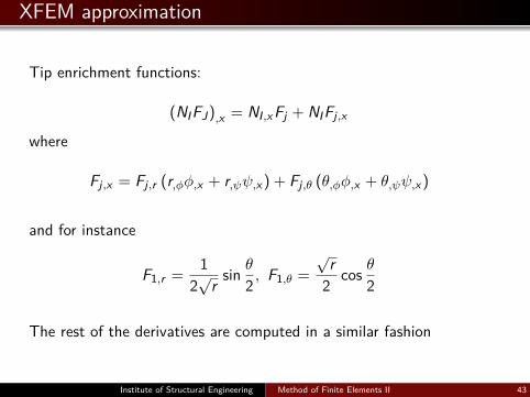
Tip enrichment functions:
(NIFJ),x = NI,xFj + NIFj,x
where
Fj,x = Fj,r (r,φφ,x + r,ψψ,x ) + Fj,θ (θ,φφ,x + θ,ψψ,x )
and for instance
F1,r = 12√
r sin θ2 , F1,θ =√
r2 cos θ2
The rest of the derivatives are computed in a similar fashion
Institute of Structural Engineering Method of Finite Elements II 43

Discrete equilibrium equations
The discrete equilibrium equations are obtained by plugging theshape function derivatives into the weak form:∫
Ωδε : D : ε dΩ =
∫Ωδu · b dΩ +
∫Γtδu · t dΓ
where:
ε are the strains obtained through the shape functionderivatives
D is the Hooke tensoru are the displacements obtained through the XFEM
approximationb, t are body forces and tractions
Institute of Structural Engineering Method of Finite Elements II 44

Discrete equilibrium equations
From the above the usual system of equations results:
Kun = f
with the following structure: Kuu Kua Kub
Kau Kaa Kab
Kbu Kba Kbb
u
ab
=
fu
fa
fb
where elements of the stiffness matrix are obtained as:
KklIJ =
∫Ω
(Bk
I
)TDBl
JdΩ, k, l = u, a, b
Institute of Structural Engineering Method of Finite Elements II 45
Discrete equilibrium equations
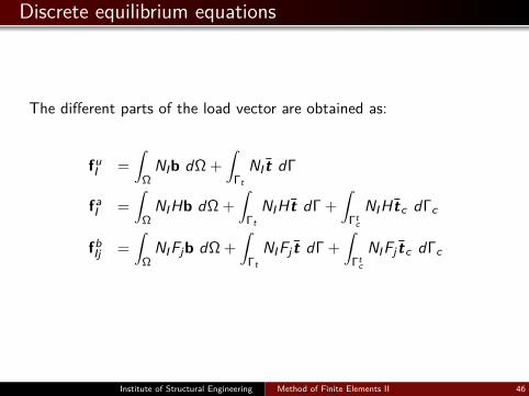
The different parts of the load vector are obtained as:
fuI =
∫Ω
NIb dΩ +∫
ΓtNI t dΓ
faI =
∫Ω
NIHb dΩ +∫
ΓtNIH t dΓ +
∫Γt
c
NIH tc dΓc
fbIj =
∫Ω
NIFjb dΩ +∫
ΓtNIFj t dΓ +
∫Γt
c
NIFj tc dΓc
Institute of Structural Engineering Method of Finite Elements II 46

Numerical integration
In order to obtain the stiffness matrix and load vectors for theenriched approximation:
Discontinuous and singular functions need to be integrated
Usual Gauss integration cannot be used since it is only accuratefor polynomials
Element partitioning and special transformations are typicallyemployed
Institute of Structural Engineering Method of Finite Elements II 47

Numerical integration - Jump enrichment
Jump enriched elements are integrated using element partitioning:
Gauss point Integration element
FE approximation
of the crack
Crack
Institute of Structural Engineering Method of Finite Elements II 48

Numerical integration - Jump enrichment
For tip enriched elements polar integration is typically employed:
Institute of Structural Engineering Method of Finite Elements II 49

Enrichment shifting
By reviewing the displacement approximation:
u (x) =∑
I∈N NI (x) uI +∑
J∈N j NJ (x) H (φ) aJ +∑
T∈N t∑
j NT (x) Fj (r , θ) bTj
we observe that:
Enrichment functions do not vanish at nodal points
The standard FE dofs do not correspond to nodal displacements
Institute of Structural Engineering Method of Finite Elements II 50

Enrichment shifting
This can be fixed by employing “shifted” enrichment functions:
u (x) =∑I∈N
NI (x) uI +∑
J∈N j
NJ (x) (H (φ)− H (φJ)) aJ+
+∑
T∈N t
∑j
NT (x) (Fj (r , θ)− Fj (rT , θT )) bTj
The nodal values of the enrichment functions are subtractedfrom the enrichment functions themselves
Enrichment functions vanish at nodal points
Standard FE dofs correspond to nodal displacements
Institute of Structural Engineering Method of Finite Elements II 51

Stress Intensity Factors
Stress intensity factors are typically obtained using the interactionintegral:
I =∫A
[(σaux : ε) e1 −
(σ · ∂uaux
∂x + σaux · ∂u∂x
)]∇qdA
In the above:
Stress, strain and displacement fields are obtained from theXFEM solutionAuxiliary fields are obtained from the Westergaard solutionA system of coordinates defined from the LS gradients is usedFunction q needs to be defined
Institute of Structural Engineering Method of Finite Elements II 52

Stress Intensity Factors
To define q:
A radius rd is selectedNodes within that radius fromthe crack tip are given a valueqI = 1Nodes outside that radius aregiven a value qI = 0Values in the element interiorsare interpolated using the FEshape functions:
q =∑
INIqI
Interaction integral domain
q
crack
rd
Institute of Structural Engineering Method of Finite Elements II 53

Solution overview
The level sets are initialized for an initial crack geometry
The displacement, stress and strain fields are obtained withXFEM
SIFs are computed, the fracture criterion (e.g. the maximumcircumferential stress criterion) is evaluated and the propagationdirection is computed
The crack is propagated by an increment in the computeddirection
The LS crack description is updated
The procedure is repeated for several steps
Institute of Structural Engineering Method of Finite Elements II 54

Comparison to FEM
FEM and XFEM solution of a problem involving discontinuities andsingularities along moving interfaces (e.g. crack propagation):
Domain
Institute of Structural Engineering Method of Finite Elements II 55

Comparison to FEM
FEM and XFEM solution of a problem involving discontinuities andsingularities along moving interfaces (e.g. crack propagation):
Initial mesh
Institute of Structural Engineering Method of Finite Elements II 55

Comparison to FEM
FEM and XFEM solution of a problem involving discontinuities andsingularities along moving interfaces (e.g. crack propagation):
Crack appears → Re-meshing and mesh refinement is required
Institute of Structural Engineering Method of Finite Elements II 55

Comparison to FEM
FEM and XFEM solution of a problem involving discontinuities andsingularities along moving interfaces (e.g. crack propagation):
Crack propagates → Re-meshing is required
Institute of Structural Engineering Method of Finite Elements II 55

Comparison to FEM
FEM and XFEM solution of a problem involving discontinuities andsingularities along moving interfaces (e.g. crack propagation):
Crack propagates → Re-meshing is required
Institute of Structural Engineering Method of Finite Elements II 55

Comparison to FEM
FEM and XFEM solution of a problem involving discontinuities andsingularities along moving interfaces (e.g. crack propagation):
Crack propagates → Re-meshing is required
Institute of Structural Engineering Method of Finite Elements II 55

Comparison to FEM
FEM and XFEM solution of a problem involving discontinuities andsingularities along moving interfaces (e.g. crack propagation):
Crack propagates → Re-meshing is required
Institute of Structural Engineering Method of Finite Elements II 55

Cohesive zone models
In those models some forces are introduced which resist separation ofthe surfaces:
Those forces gradually reduce to a value of zero which correspondsto full separation
Institute of Structural Engineering Method of Finite Elements II 56

Weak form
The weak form in the presence of cohesive forces becomes:
∫Ωδε : D : ε dΩ︸ ︷︷ ︸
fint
+∫
Γcδ(u+ − u−
)· tc dΓc︸ ︷︷ ︸
−fc
= λ
∫Γtδu · t dΓ︸ ︷︷ ︸fext
where:
tc are the cohesive forces: tc = τcnn is the normal vector to the crack surface
u+,u− are the displacements at the two crack facesλ is a load factor
Institute of Structural Engineering Method of Finite Elements II 57

Enrichment functions
The modified step function is used for jump enrichment
Several alternatives have been proposed for tip enrichment, forinstance:
Fj (r , θ) = r sin θ2 or r3/2 sin θ2 or r2 sin θ2
we observe that a singularity is not present in this type offracture!
Institute of Structural Engineering Method of Finite Elements II 58
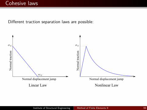
Cohesive laws
Different traction separation laws are possible:
Linear Law
Normal displacement jump
Norm
al t
ract
ion
Nonlinear Law
Normal displacement jumpN
orm
al t
ract
ion
Institute of Structural Engineering Method of Finite Elements II 59

Integration of cohesive forces
Cohesive forces:
Have to be integrated along the crack faces
Are non linear functions of the displacements
Introduce a non linearity even for linear elastic materials
Institute of Structural Engineering Method of Finite Elements II 60

Nonlinear solution
During the nonlinear solution the load factor needs to bedetermined
An additional condition is needed for the determination of theload factor
Usually one of the following conditions is used:
The mode I SIF at the tip should be zero: g = KI = 0
The stress projection normal to the surface of the crack shouldbe equal to the tensile strength of the material:g = n · σ · n− σc = 0
Institute of Structural Engineering Method of Finite Elements II 61

SIFs and propagation direction
Stress Intensity Factors are obtained using a modified version ofthe interaction integral
The propagation direction is determined using a criterion suchas the maximum circumferential stress criterion
Institute of Structural Engineering Method of Finite Elements II 62

Nonlinear solution
The residual and tangent stiffness for the Newton-Raphson methodare:
K− ∂fc∂u −fext
∂g∂u 0
· [ uλ
]= −
[Ku− λfext − fc
g
]
We observe the similarities to arc length methods!
Institute of Structural Engineering Method of Finite Elements II 63

Solution overview
Given an initial crack the displacements and load factor arecomputed using the nonlinear solution method presented
SIFs are computed and the direction of propagation is obtainedusing the maximum circumferential stress criterion
The crack is propagated by an increment in the computeddirection
The procedure is repeated for as many crack propagation stepsas needed
Institute of Structural Engineering Method of Finite Elements II 64

Extension to 3D
The methods presented mostly apply to 2D crack propagation
Extension of the discretization schemes (XFEM) isstraightforward
Extension of the fracture mechanics methods (failure criteriaetc.) is somehow more involved
Several alternatives exist in the literature each with itsrespective advantages and drawbacks
Institute of Structural Engineering Method of Finite Elements II 65