Writing Sample

Forecasting Project Homework 4

Yiqun Li

Macroeconometrics Ai Deng April 2015

Forecasting Project ii

Table of Contents

Overview of the Data ....................................................................................................... 1

Autoregressive Estimation ................................................................................................ 3

AR(12) ............................................................................................................................................... 3

AR(12) with Time Trend ..................................................................................................................... 4

ARMA ............................................................................................................................................... 5

Volatility Adjustment ....................................................................................................... 6

Accelerating Growth ........................................................................................................................... 6

Month-to-month Changes ................................................................................................................... 7

Forecast for 2007 ............................................................................................................. 8

Yiqun Li

Macroeconometrics Ai Deng

April 2015

Forecasting Project 1

Forecasting Project Homework 4

This paper briefly discusses how I used macroeconometric techniques to forecast the data of all 12 months 2007, given a time series data ranging from Jan 1996 to Dec 2006. Before the projection, I had no knowledge of what was the source of the data.

The performance of the forecast is shown in the appendix. The paper is composed by three sections, beginning with an overview of the data, which is followed by autoregressive estimation, and finally a volatility/variance adjustment. I used Stata 13 to complete all the graphing and computation.

Overview of the Data

Before applying any econometrical or statistical techniques, it is necessary to take an overview of the data, which serves as a shortcut to determine what forecasting models will

1000

0020

0000

3000

0040

0000

Y

1992m1 1994m1 1996m1 1998m1 2000m1 2002m1 2004m1 2006m1month

Graph 1


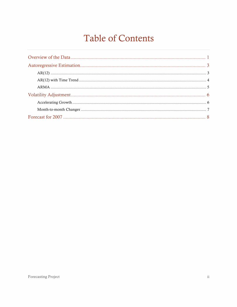
be more efficient and unbiased.

Graph 1 plots the data from 1996 to 2006. From this graph, it is easy to draw two preliminary conclusions:

1. There is a seasonal pattern with increasing trend. 2. The volatility/variance is increasing.

We observe from the graph that each season consists of 12 periods. To confirm this preliminary conclusion, simply find the AC and PAC of the variable.

-1 0 1 -1 0 1 LAG AC PAC Q Prob>Q [Autocorrelation] [Partial Autocor] ------------------------------------------------------------------------------- 1 0.8582 0.8945 134.8 0.0000 |------ |------- 2 0.8196 0.3711 258.42 0.0000 |------ |-- 3 0.8267 0.4129 384.92 0.0000 |------ |--- 4 0.8251 0.3453 511.64 0.0000 |------ |-- 5 0.8176 0.3730 636.78 0.0000 |------ |-- 6 0.7884 0.2241 753.79 0.0000 |------ |- 7 0.7844 0.3617 870.3 0.0000 |------ |-- 8 0.7588 0.2498 979.98 0.0000 |------ |- 9 0.7295 0.1502 1081.9 0.0000 |----- |- 10 0.6871 -0.2350 1172.9 0.0000 |----- -| 11 0.6986 -0.1914 1267.5 0.0000 |----- -| 12 0.8003 0.9617 1392.4 0.0000 |------ |------- 13 0.6681 -0.4277 1480 0.0000 |----- ---| 14 0.6311 -0.2593 1558.6 0.0000 |----- --| 15 0.6330 -0.3428 1638.1 0.0000 |----- --|

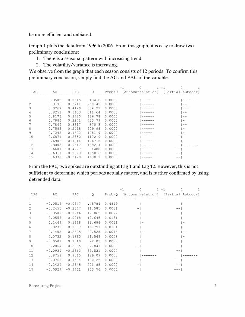
From the PAC, two spikes are outstanding at Lag 1 and Lag 12. However, this is not sufficient to determine which periods actually matter, and is further confirmed by using detrended data.

-1 0 1 -1 0 1 LAG AC PAC Q Prob>Q [Autocorrelation] [Partial Autocor] ------------------------------------------------------------------------------- 1 -0.0516 -0.0547 .48784 0.4849 | | 2 -0.2456 -0.2647 11.585 0.0031 -| --| 3 -0.0509 -0.0946 12.065 0.0072 | | 4 0.0558 -0.0218 12.645 0.0131 | | 5 0.1469 0.1328 16.684 0.0051 |- |- 6 0.0239 0.0587 16.791 0.0101 | | 7 0.1405 0.2605 20.528 0.0045 |- |-- 8 0.0732 0.1860 21.549 0.0058 | |- 9 -0.0501 0.1019 22.03 0.0088 | | 10 -0.2864 -0.2995 37.841 0.0000 --| --| 11 -0.0934 -0.2863 39.531 0.0000 | --| 12 0.8758 0.9565 189.09 0.0000 |------- |------- 13 -0.0768 -0.4584 190.25 0.0000 | ---| 14 -0.2424 -0.2845 201.85 0.0000 -| --| 15 -0.0929 -0.3751 203.56 0.0000 | ---|


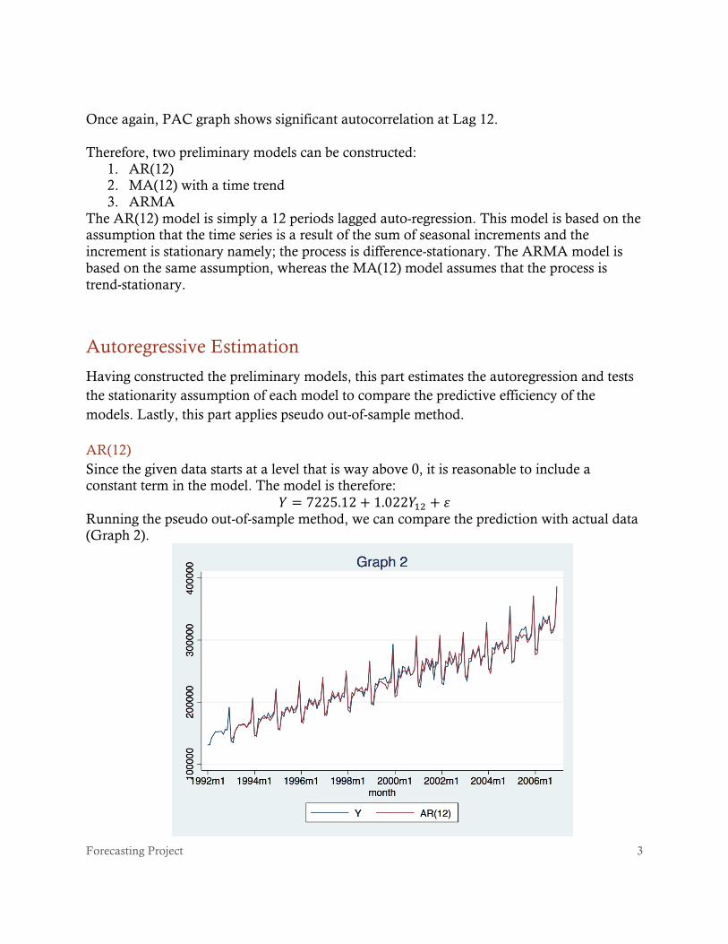
Once again, PAC graph shows significant autocorrelation at Lag 12. Therefore, two preliminary models can be constructed:

1. AR(12) 2. MA(12) with a time trend 3. ARMA

The AR(12) model is simply a 12 periods lagged auto-regression. This model is based on the assumption that the time series is a result of the sum of seasonal increments and the increment is stationary namely; the process is difference-stationary. The ARMA model is based on the same assumption, whereas the MA(12) model assumes that the process is trend-stationary.

Autoregressive Estimation

Having constructed the preliminary models, this part estimates the autoregression and tests the stationarity assumption of each model to compare the predictive efficiency of the models. Lastly, this part applies pseudo out-of-sample method.

AR(12) Since the given data starts at a level that is way above 0, it is reasonable to include a constant term in the model. The model is therefore:

𝑌 = 7225.12+ 1.022𝑌!" + 𝜀 Running the pseudo out-of-sample method, we can compare the prediction with actual data (Graph 2).


Noticeably, this model overall fits the actual well; however, it performs unsatisfactorily in predicting the month-to-month change in a year, which is also the most difficult part to predict. Though we may be able to tell whether there will be a climb or a fall from one month to another, it is hard to tell the extent. Conceivably, this issue will also occur in the MR(12) model. To address the issue, it is necessary to analyze the volatility of the data, which will be discussed later. To test whether the process is difference stationary, simply use Dickey-Fuller test on the first difference of the original data. Dickey-Fuller test for unit root Number of obs = 178 ---------- Interpolated Dickey-Fuller --------- Test 1% Critical 5% Critical 10% Critical Statistic Value Value Value ------------------------------------------------------------------------------ Z(t) -20.034 -3.484 -2.885 -2.575 ------------------------------------------------------------------------------ MacKinnon approximate p-value for Z(t) = 0.0000

According to the test results, the process is difference stationary; therefore, the AR(12) model is reasonable.

AR(12) with Time Trend This model is basically an MA model that assumes the data are just a time series that fluctuate along a time trend.

𝑌 = −243136.3+ 1003.476𝑡 + 𝛾 𝛾 = .982016𝛾!" + 𝜀

Again, using the pseudo-out-of-sample method (Graph 3):


We can see that compared to AR(12) model, the MR(12) with time trend is more deviant from the real data. The MA(12) term in the model has a coefficient of 0.98, which is less than 1. This is contrary to our observation that the deviation from the time trend becomes larger across time. Besides, the moving-average term does not estimate efficiently as it treats all observations equally. It is reasonable to assume that when the process comes to a peak, the deviation from its linear estimation is greater. This model is therefore abandoned.

ARMA This autoregressive-moving-average model consists of a lag 12 autoregressive term and a lag 12 moving-average term. This model basically substitutes the time trend with an autoregressive term.

𝑌 = 237695.6+ 0.9797656𝑌!" + 𝛾 𝛾 = 0.6399572𝛾!" + 𝜀

The original data is non-stationary whereas in this estimation, the coefficient of the autoregressive term is smaller than 1. Even though it is very close to 1, we see it slow down the growth of the pseudo-out-of-sample forecast (Graph 4):

The gap between the forecast and the real data become lager, this indicates that the estimation is biased. The model is therefore biased.

After comparing all the alternatives, AR(12) model appears to be the most efficient model, based on which we make adjustment for volatility.


Volatility Adjustment

The following table shows that the standard deviation of each year has increased since the beginning of the given time series.

1992|15294.081 1993|17866.066 1994|19212.123 1995|18420.228 1996|17466.754 1997|17656.24 1998|20267.972 1999|23834.002 2000|19410.558 2001|20375.55 2002|21268.23 2003|23225.521 2004|25354.954 2005|27391.494 2006|25503.455

Two behaviors of the process can explain such phenomenon:

• Accelerating growth. • Enlarging month-to-month changes.

Accelerating Growth To test if there is an accelerating growth, simply introduce a squared autoregressive term into the original AR(12) model. This yields the following estimation: Source | SS df MS Number of obs = 168 -------------+------------------------------ F( 2, 165) = 5944.92 Model | 4.5624e+11 2 2.2812e+11 Prob > F = 0.0000 Residual | 6.3314e+09 165 38371828.8 R-squared = 0.9863 -------------+------------------------------ Adj R-squared = 0.9861 Total | 4.6257e+11 167 2.7699e+09 Root MSE = 6194.5 ------------------------------------------------------------------------------ Y | Coef. Std. Err. t P>|t| [95% Conf. Interval] -------------+---------------------------------------------------------------- Y | L12. | .9496485 .0748648 12.68 0.000 .8018322 1.097465 | Y_squared | L12. | 1.58e-07 1.61e-07 0.98 0.329 -1.60e-07 4.75e-07 | _cons | 15211.37 8435.846 1.80 0.073 -1444.753 31867.49 ------------------------------------------------------------------------------

The coefficient for the squared autoregressive term is very close to zero and insignificant. It is therefore reasonable to say that the growth is steady, and the increasing volatility is not due to an accelerating growth.


Month-to-month Changes To test if the month-to-month changes are truly enlarging, simply run a stationarity test on the absolute month-to-month changes. If it is not stationary, then month-to-month changes can hardly explain the increasing volatility.

To perform the test, take the absolute values of month-to-month changes first and then use Augmented Dickey-Fuller test. DF-GLS mu 1% Critical 5% Critical 10% Critical [lags] Test Statistic Value Value Value ------------------------------------------------------------------------------ 13 1.189 -2.589 -1.964 -1.657 12 1.150 -2.589 -1.972 -1.664 11 1.659 -2.589 -1.980 -1.672 10 -1.611 -2.589 -1.987 -1.679 9 -2.189 -2.589 -1.995 -1.686 8 -2.527 -2.589 -2.002 -1.693 7 -3.041 -2.589 -2.010 -1.700 6 -3.849 -2.589 -2.017 -1.707 5 -4.169 -2.589 -2.023 -1.713 4 -4.441 -2.589 -2.030 -1.719 3 -4.400 -2.589 -2.036 -1.724 2 -4.945 -2.589 -2.042 -1.729 1 -6.104 -2.589 -2.047 -1.734 Opt Lag (Ng-Perron seq t) = 12 with RMSE 5625.384 Min SC = 17.67238 at lag 12 with RMSE 5625.384 Min MAIC = 17.48427 at lag 12 with RMSE 5625.384

The test result proves that the month-to-month changes are not stationary.

Though we cannot firmly state that all the month-to-month changes in 2007 will be greater, we are confident to say they will increase. Therefore, we add a lag 12 first difference term in the AR(12) in order to adjust for the volatility. The regression gives us the final model:

𝑌 = 7296.199+ 1.022𝑌!" − 0.0047112𝑑𝑌!" + 𝜀


Forecast for 2007

According to this estimation, the forecast for 2007 is: 1/1/07 300036.6655 2/1/07 296234.9207 3/1/07 340786.5228 4/1/07 330978.1636 5/1/07 352252.8623 6/1/07 345596.4989 7/1/07 340576.7292 8/1/07 354092.1206 9/1/07 325187.4534 10/1/07 327431.0226 11/1/07 337816.8233 12/1/07 396156.7522

End.

Documents

Writing Sample