AO-AO91 459 AIR FORCE INST OF TECH WRIGHT-PATTERSON AFB OH F/6 12/1

DETERMINATION OF MODAL PARAMETERS FROM EXPERIMENTAL FREQUENCY R--ETC(U)

DEC 7A C MILLERUNCLASSIFIED AFITCTC 1A NL

mhhIhIIIIIIIIuIl lllllllllflEIIEIIEIIIEEIIIIIIIIIIIIIIuIEEEEEIIIIIIIEIIEEEE-EI-EII

-iii1

'111 11jW8 1 2

MICROtOPY RESOLUTION TEST CHART

NATIONAL BUREAU OF STANOARDS-1963-A

LI

I PDETERMINATION OF MODAL PARAMETERS FROM

1EXPERIMENTAL FREQUENCY RESPONSE DATA

I

I DTICfA LECTE7

NOV 1 ov ,80

APPROVED:

,f.!.

, I r-iiApproved fo- 1u-i rodeaseO

Distrbun tlmio d

i i " E.,.... .C0

UNCLASSIFIEDSECURITY CLASSIFICATION OF THIS PAGE (no'n Date Entered) __________________

REPORT DOCUMENTATION PAGE READ INSTRUCTIONS

I REPORT NUMBER 12. GOVT ACCESSION No. 3. =R -

79-1 82T

TI6 Onete$intionfl dcaelT~ S. TYPE 0 RC NRT & PERIOD COVERED

Experimental Frequency Response Data. Thesis

V ~6. PERFORMING 0OR0. REPORT NUMBER

7. AUTHOR(*)S.CNRCORGATUME)

Clarence Walter Miller -41A:

9PERFORMING ORGANIZATION NAME AND ADDRESS 10. PROGRAM ELEMENT, PROJECT. TASK

AFIT student at: The University of Texas atAustinII

1I. CONTROLLING OFFICE NAME AND ADDRESS t"2 i10

WPAFB OH 45433 0127 MEOPAGES .314. MONITORING AGENCY NAME A ADDRESS(if different from Controling Office) 1S. SECURITY CLASS. (of thia Ls WI

Unclassified15. DECL ASS# FICATION/oowN rRAOING

SCHEDULE

16. DISTRIBUTION STATEMENT (of this Report)Approved for public release; distribution unlimited

17. DISTRIBUTION STATEMENT (of the abstract entered In Block 20, if different from Report)

Al~ ~ 6V O 10 REI SE AFR 190.17.

n=U''C- LYNC"1,M USAF

19. KEY WORDS (Continue on reverse side it necessary and Identify by block number)

20. ABSTRACT (Continue on reverse aide It necesary and Identify by block number)

Attached

J DD I JAN 73 1473 EDITION OF I NO0V 65 1S OBSOLETE (-7~ siSECURITY CLASSIFICATION OF THIS PAGE (Mont Datotes e9

SECURITY CLASSIFICATION OF THIS PAGI(Wh n Data Engar)*

SECURITY CLASSIFICATION OF ? PAGEt'Whn Dot* ffnteroE)

. . .. . .. IL

b.

K; ABSTRACT

In recent years, a number of advances have been

made in determining the dynamic properties of a struc-

ture. These advances have opened the field of modal

analysis, the term used to describe the use of experi-

mental frequency response data to determine the modal

properties of natural frequencies, damping ratios, and

mode shapes. One of the main problems in the area of

modal analysis is the lack of complete documentation

for the techniques in use. The purpose of this thesis

is to investigate some of the modal analysis techniques

in use, and to document, fully, the assumptions and

the equations and computer algorithms associated with

each method. Three curve fitting techniques are pre-

sented along with some example problems which demon-

strate the limitations of each method

iv

L

DETERMINATION OF MODAL PARAMETERS FROM

EXPERIMENTAL FREQUENCY RESPONSE DATA

I by

I CLARENCE WALTER MILLER, B.S.A.S.E.

j THESIS

Presented to the Faculty of the Graduate School of

I The University of Texas at Austin

Iin Partial Fulfillment Accession For

of the Requirements DCTISA I

for he egre ofUnannouncedfor the Degree ofJust ificaticn____

MASTER OF SCIENCE IN ENGINEERING :By________I Distr ibu*oic-L*vail91! ly oeI Avail and/or

Dist., special

I THE UNIVERSITY OF TEXAS AT AUSTIN

December 1978

I ACKNOWLEDGEMENTS

SI

The author would like to express his gratitude

I for the assistance of Dr. Craig Smith throughout this

project. His insight and guidance were invaluable.

I Also of considerable help were the comments of Joe

IThornhill of IBM.The author would also like to thank Capt.

1Samuel Brown of the Air Force Institute of Technologyfor his efforts in the management of the author's

I education program.

IC. W. M.

December, 1978

iii

III____

TABLE OF CONTENTS

Page

ACKNOWLEDGEMENTS............ . . ... .. .. . . ...

ABSTRACT. ............. .......... v

CHAPTER

I. INTRODUCTION. . ................ 1

II. THE STRUCTURAL DYNAMIC MODEL .. ........ 7

2.1 Assumptions .. .............. 7

2.2 The Transfer Matrix .. .......... 8

2.3 Modes of Vibration ............10

2.4 Complex Mode Shapes. ........... 17

2.5 Deriving Mass, Stiffness, andDamping Matrices FromFrequency Response Data. ........ 19

2.6 Summary. ................. 24

III. MODAL PARAMETER ESTIMATION TECHNIQUES . 26

3.1 Parameter Identification ......... 26

3.2 Single Degree of FreedomTechniques ...............29

3.2.1 Quadrature ResponseTechnique ............29

V

I

* vi

Page

3.2.2 Method of Kennedy and* Pancu .. ........... ... 32

3.3 Multi Degree of Freedom CurveFitting .... .............. ... 46

3.3.1 Complex Curve Fit ...... . 46....

3.3.2 Curve Fitting of QuadratureResponse .. .......... ... 57

3.4 Summary .... ............... ... 63

IV. EXAMPLES OF CURVE FITTING TECHNIQUES . . 64

4.1 Introduction ... ............ . 64

4.2 Example Problem One .. ......... ... 65

4.2.1 Method of Kennedy andPancu .. ........... ... 66

4.2.2 Complex Curve Fit ...... . 71

4.2.3 Curve Fit of Imaginary Partof H(jw) .. .......... ... 73

4.3 Example Problem Two .. ......... ... 76

4.3.1 Method of Kennedy andPancu .. ........... ... 77

4.3.2 Complex Curve Fit ... ...... 84

4.3.3 Curve Fit of Imaginary Partof H(jw) .. .......... ... 85

4.4 Determination of Mass, Stiffness, andDamping Matrices . ......... ... 87

4.5 Summary .... ............... ... 89

V. SUMMARY AND CONCLUSIONS ......... 91

vii

Page

APPENDIX A - CIRCLE FIT ALGORITHM .... ...... 96

APPENDIX B - MULTI DEGREE OF FREEDOM CURVEFIT ALGORITHM .. ........... 101

APPENDIX C - IMAGINARY CURVE FIT ALGORITHM . . .. 105

APPENDIX D - DATA. ................. 111

BIBLIOGRAPHY .. ................... 127

VITA

CHAPTER I

INTRODUCTION

The use of experimental methods to determine

the dynamic characteristics of a system or structure

has become widely used and accepted during the 1970's,

primarily because of the advances in digital test

equipment. The use of these methods has become com-

monly known as modal analysis. Experimental modal

analysis provides the ability to pinpoint vibration

problems by showing troublesome frequencies, damping

factors, and mode shape data which can be used by a

designer to pinpoint weak spots in a structure.

In order to obtain meaningful answers to vi-

bration problems, it is essential that an adequate

mathematical model be selected. If a model is avail-

able, there are methods which can be used for com-

puting the dynamic response of the structure. However,

if the parameters, i.e., mass, stiffness, and damping,

are not known, or if the model itself is not known,

then the solutions cannot be obtained. One approach

to modeling is through the use of transfer functions.

If the applicable transfer functions can be determined,

1

2

then the response to any input can be determined.

One advantage in using the transfer function approach

is that only those points of a structure which are of

interest need be considered. The determination of

these transfer functions is the main thrust in exper-

imental modal analysis.

In general, modal analysis involves the de-

scription of the dynamic characteristics of a struc-

ture by observing its natural modes of vibration and

the associated modal properties, i.e., frequency and

damping ratio. Natural frequency and damping ratio

are global properties of the system and consequently

can be measured at almost any point on the system.

The key to reliable modal parameter estimates is the

accurate measurement of transfer functions of the sys-

tem. The transfer function is a complex valued func-

tion. The Laplace transform is used to characterize

the transfer function because it can be used to con-

vert a measured frequency response function into a

partial fraction expansion with each partial fraction

containing information on each resonance of the sys-

tem in the frequency range of analysis. The frequency

response function, which is the ratio of the output to

the input (assumed here to be the ratio of output dis-

3

placement to input force) evaluated along the jw fre-

quency axis, can be used to determine the frequency,

damping, magnitude, and phase of each resonance.

The purpose of this thesis is not to describe

the techniques used in obtaining the frequency re-

sponse function, but rather to explore three methods

of extracting the modal parameters from the measured

data and to point out the advantages and disadvan-

tages of each method. For a description on frequency

response measurement techniques in mechanical systems,

the reader is directed to references (10) and (11).l

For a brief review of the literature, prior

to 1968, concerning the modeling, or measuring, of

the transfer function, the reader is referred to a

PhD dissertation by William R. Shapton, (15). Shapton

discusses briefly the problems with earlier attempts

at transfer function measurement. Some of the earlier

works reviewed by Shapton include Savant (14),

Chestnut and Mayer (2), Crafton (3), Tse, Morse, and

Hinkle (17), Jacobsen and Ayre (5), Brooks (1),

Simmons (16), and many others. Shapton's work was

tFrom this point on, the nomenclature (will be used to denote a reference number in thebibliography.

-- - . ---.~v--..--. .-. A

4

in the development of procedures for predicting the

response versus time of surface strain of a complex

structure resulting from a dynamic excitation. His

assumptions were that the structure was capable of

being represented as a linear system with time in-

variant parameters, and that the system could be ap-

proximated by a finite number of ordinary differential

equations with constant coefficients. He also as-

sumed that the system was underdamped and that the

damping could be represented as an equivalent vis-

cous damping. Shapton presents a method to determine

the transfer function by extracting it in analytical

form from the experimentally determined frequency

response data.

Most of the works performed in the area of

deriving transfer functions from experimental data

have as their initial basis, a method presented by

Kennedy and Pancu (6). Kennedy and Pancu presented

one of the first papers on determining modal charac-

teristics from test data. The object of their paper

was to bring out an awareness of the phase relation-

ship in trying to correlate between measured and

calculated modes. They presented a technique to

identify normal modes from polar plots (plot of re-

iJ

5

sponse vector with forcing frequency) of the fre-

quency response function. The basis for this tech-

nique is that near a resonant frequency the polar plot

will approximately describe a circle (for a single

mode). This method will be discussed further in a

later section of this thesis.

A more recent work in this area was done by

Klosterman (8). He presented new methods to determine

a complex modal representation from experimental data.

He generalized the method of Kennedy and Pancu to

include the case where damping is not proportional to

the stiffness or mass.

Using Klosterman's work, more recent papers

by Richardson (11) and Potter and Richardson (9) have

presented the basis for measuring transfer functions

using a least squares estimator to measured frequency

response data.

This thesis will discuss the circle fit

method of Kennedy and Pancu, and two other curve fit

techniques, one which uses the total response curve,

and one which uses only the imaginary part of the

response. Chapter II presents the dynamic model

used for an elastic structure and the compliance

transfer function for the structure in the Laplace

I

6

domain. Chapter III discusses four methods of ex-

tracting the desired modal parameters from the fre-

quency response function. Chapter IV will present

two example problems using three of the methods dis-

cussed in Chapter III. And finally, Chapter V is the

summary and conclusions of the methods discussed.

CHAPTER II

THE STRUCTURAL DYNAMIC MODEL

2.1 Assumptions

In most problems in modal analysis, the model

is assumed to be described by a system of n simulta-

neous second order linear differential equations. In

the time domain these equations are given by

M R + C * + K x = f (t) (2.1)

where

x (t) - n-dimensional displacement vector

f (t) = n-dimensional force vector

M = n x n mass matrix

C= n x n damping matrix

K - n x n stiffness matrix

For the purpose of this thesis, it is assumed that

the matrices M, C, and K are real valued and sym-

metric. The energy associated with the mass and

stiffness matrices is stored and can always be re-

covered, however, the energy associated with the

damping is dissipated and is lost from the system.

7

8

The damping mechanism in this formulation is assumed

to be viscous, i.e., damping force is proportional to

velocity. In practice, most mechanical structures ex-

hibit rather complicated damping mechanisms, however,

Richardson and Potter (13) have shown that all of the

damping mechanisms can be modeled in terms of energy

dissipation by an equivalent viscous damper.

2.2 The Transfer Matrix

The Laplace transform of equation (2.1) yields

M [s 2 X(s) - sx(o) - x(o)] + C [sX(s) - x(o)]

+ K X(s) = F(s) (2.2)

Assuming that the initial conditions are zero (or al-

ternately combine them with F(s)), the transformed

equations become

[_2 + Cs + K] X(s)- F(s) (2.3)

Defining B(s) as the system matrix,

B(s) - Ms2 + Cs + K (2.4)

then equation (2.3) can be written as

B(s) X(s) - F(s) (2.5)

9

B(s) is often referred to as the dynamic flexibility

of the structure.

Now define H(s) as the inverse of B(s) (as-

suming that the inverse exists). Then equation (2.5)

becomes

x(s) - H(s) F(s) (2.6)

H(s) is the n x n transfer matrix, each element of

which is a transfer function, i.e., hij is the trans-

fer function which relates the response at point i due

to an excitation at point j. Because of reciprocity

hij - hji for all i and j. Taking a closer look at

each element of H(s) reveals that each is a rational

fraction in s, i.e.,

b S2n-2 + b2 s2n-3 +

hij det B(s)

+ b n. s + bn.S2n-2 sb2n-1det B(s) (2.7)

where

det B(s) - determinant of B(s)

The roots of det B(s) are called the poles of H(s) and

are the values of s for which det B(s) - 0.

If we assume that the poles of H(s) are dis-

i

10

tinct, i.e., each of multiplicity one, and that all

modes are underdamped, each element of H(s) can be

expanded into a partial fraction form to give

n*H s) + . (2.8)s - sk s - skk i

where

sk = kth pole of H(s)

sk = complex conjugate of sk

Ak = complex residue matrix of H(s) evaluated

at s = s k

- complex conjugate of

Each k can be found by multiplying H(s) by (s - sk)

and then evaluating the result at s = sk o as long as

the poles are distinct.

2.3 Modes of Vibration

The resonant poles are the locations where

- sk . These poles can be expressed as

S k - k + Jwk

where

ak - the modal damping coefficient of the

kth mode

wk " the damped natural frequency of the

kth mode

The undamped natural frequency is given by

J 2 2k + Wk

and the damping ratio is given by

ak

k S k

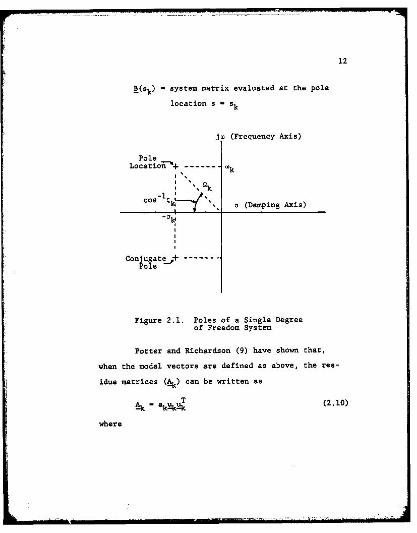
Each complex conjugate pair of poles (sk and

s) corresponds to a mode of vibration in the struc-

ture. Figure 2.1 shows the poles for a single degree

of freedom system as viewed looking down on the s-

plane.

Modal vectors, or mode shapes, are defined as

solutions to the homogeneous equation

(sk) k = 0 (2.9)

where

k - n-dimensional, complex valued modal

vector

12

- system matrix evaluated at the pole

location s - sk

jw (Frequency Axis)

PoleLocation- ------- -k

I %

Cos a (Damping Axis)

-aN

Conjugate .+Pole

Figure 2.1. Poles of a Single Degreeof Freedom System

Potter and Richardson (9) have shown that,

when the modal vectors are defined as above, the res-

idue matrices (A) can be written as

a T (2.10)

where

.~- -ON

13

ak = complex valued scaler

k T - an n x n complex valued, symmetric

matrix

In other words, the residue matrix, , can be deter-

mined, to within a multiplicative constant (complex

valued), by a mode shape vector !k, which is the so-

lution to the homogeneous equation (2.9).

Using equation (2.10), the transfer matrix

H(s) can now be written in the form

H1(s) ak!klh (2.11)H~s =s - s kk-1

or it can be written as a summation of n-conjugate

pairs

n T *T

Hs[+ (2.12)Zs - sk s - s k

k- 1

Equations- (2.11) and (2.12) are the forms of the

transfer function from which all the desired modal

parameters (frequency, damping ratio, mode shape) can

be extracted.

Potter and Richardson (9), and also (11),

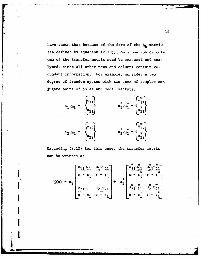
14

have shown that because of the form of the A matrix

(as defined by equation (2.10)), only one row or col-

umn of the transfer matrix need be measured and ana-

lyzed, since all other rows and columns contain re-

dundant information. For example, consider a two

degree of freedom system with two sets of complex con-

jugate pairs of poles and modal vectors.

1 .'.2 =

Expanding (2.12) for this case, the transfer matrix

[: can be written as

u 1 2Ull U1 lU21 U 1Ul UllU21

i!s- sI s - s5 -l sI - s

I

: H(s)-"a1 + aI * * * *I u21Ull u21u21 u21U1 l u21u21

- 1 1}

ILI1 1

Is - s ' * - - s S

15

m -- -- * * * -

u 1 2 u 1 2 u 1 2U2 2 U1 2U1 2 U1 2 U2 2

s - s2 s - s2 s s2 s s2

+ a 2 + a2 * * * *

u22u12 u22u22 u22ul2 u22u22

2 - 2 s- 2 s -2

(2.13)

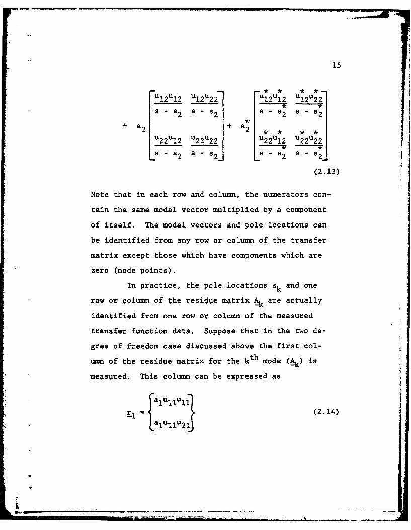
Note that in each row and column, the numerators con-

tain the same modal vector multiplied by a component

of itself. The modal vectors and pole locations can

be identified from any row or column of the transfer

matrix except those which have components which are

zero (node points).

In practice, the pole locations sk and one

row or column of the residue matrix A are actually

identified from one row or column of the measured

transfer function data. Suppose that in the two de-

gree of freedom case discussed above the first col-

umn of the residue matrix for the kth mode ( ) is

measured. This column can be expressed as

: lUllUll

-l (2.14)

alullu 21

16

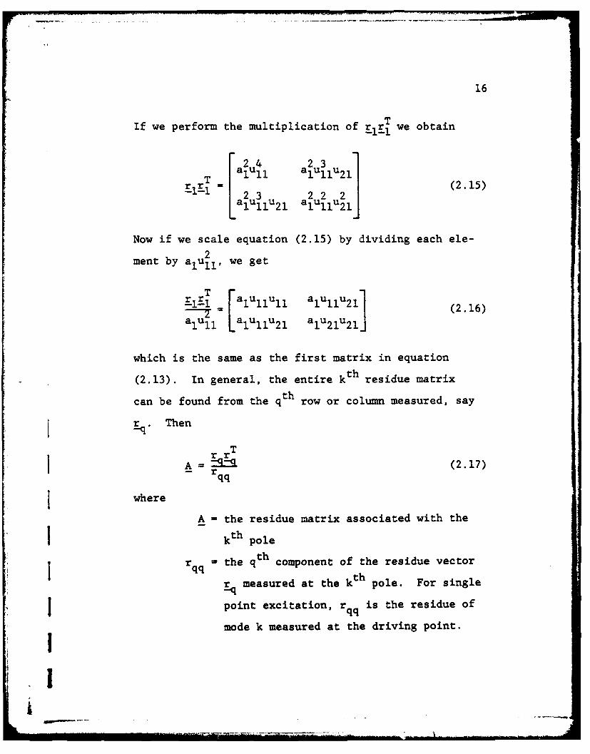
If we perform the multiplication of r r T we obtain-1-1

a2 u4 a2 3

T 11 alullu 211

ffi1 2 3 (2.15)22121 11 21alUllU21j

Now if we scale equation (2.15) by dividing each ele-2

ment by alull, we get

s---.-i l l 1 2 (2.16)

a1u11 alllU2l alu2lu2l(

which is the same as the first matrix in equation

(2.13). In general, the entire kth residue matrix

can be found from the qth row or column measured, say

ij. Then

A - q (2.17)- qq

where

A - the residue matrix associated with the

I kth pole

rqq the qth component of the residue vectorrqq

measured at the kth pole. For single

j point excitation, r is the residue ofrqq

mode k measured at the driving point.

i

17

2.4 Complex Mode Shapes

The previous development of a structural dy-

namic model required that the damping matrix be sym-

metric and real valued. If we impose no further re-

strictions on the damping assumption, then the modal

vectors will, in general, be complex valued. When the

modal vectors are real valued, all points on the struc-

ture reach their minimum or maximum values simulta-

neously. This is not the case if the modal vectors

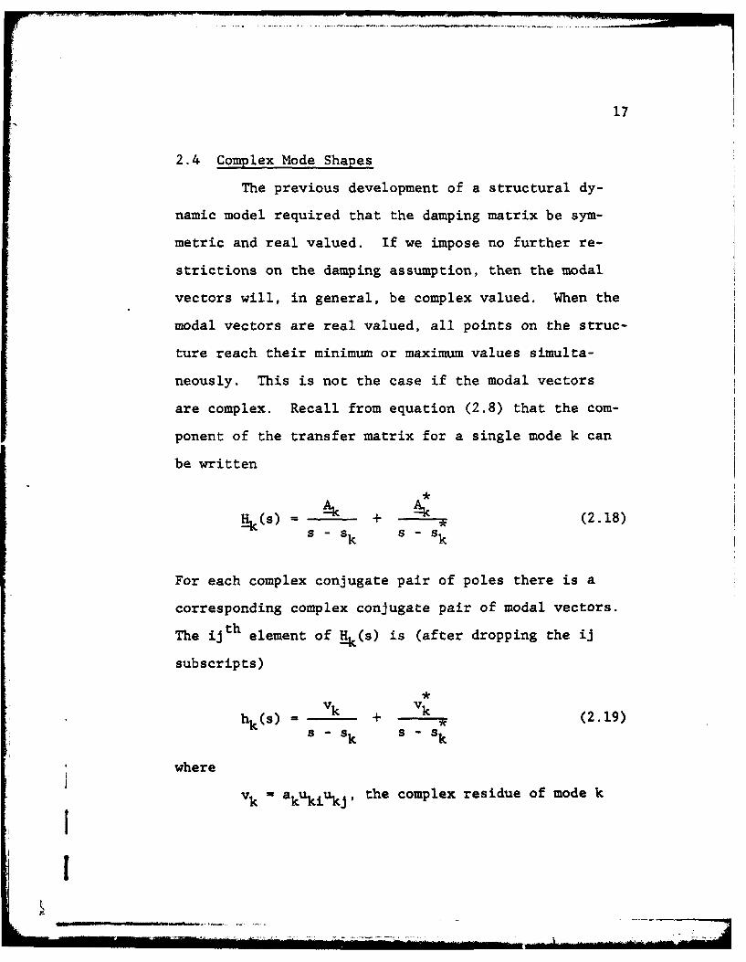
are complex. Recall from equation (2.8) that the com-

ponent of the transfer matrix for a single mode k can

be written

AA

(S) + - (2.18)s - sk S - sk

For each complex conjugate pair of poles there is a

corresponding complex conjugate pair of modal vectors.

The ij th element of Hk(s) is (after dropping the ii

subscripts)

vk vhk(s) = + vk (2.19)

s - s s - s

where

vk =akukikj , the complex residue of mode k[I

18

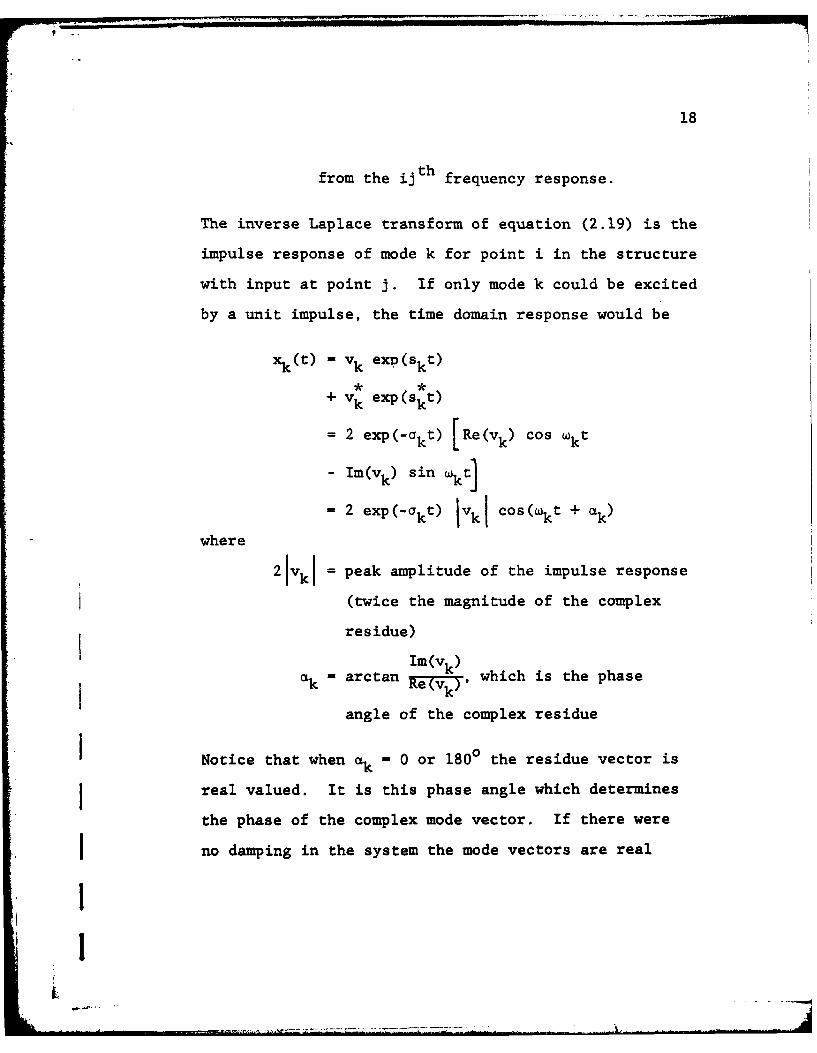
from the ij t h frequency response.

The inverse Laplace transform of equation (2.19) is the

impulse response of mode k for point i in the structure

with input at point j. If only mode k could be excited

by a unit impulse, the time domain response would be

xk(t) - vk exp(skt)

+ v, exp(skt)

=2 exp(-akt) [Re(vk) cos wkt

- Im(vk) sin wkt]

2 exp('akt) IvkI cos(Wkt + ak )

where

2IvkI = peak amplitude of the impulse response

(twice the magnitude of the complex

residue)

Im(vk)ak arctan Re(vk), which is the phase

angle of the complex residue

Notice that when ak ' 0 or 1800 the residue vector is

- real valued. It is this phase angle which determines

the phase of the complex mode vector. If there were

no damping in the system the mode vectors are real

II

19

valued and all points on the structure reach their

minimum or maximum displacement simultaneously, i.e.,0 0 .0

ak is 0 or 180 ° . When ak is an angle other than 0

or 1800 then the node lines (lines of zero displace-

ment) will not be stationary as in the undamped case.

It is this phase angle that is neglected in some

modal parameter estimation techniques. In the tech-

niques described in this thesis, this phase angle is

accounted for and does not present major problems

2.5 Deriving Mass, Stiffness, and Damping

Matrices From Frequency Response Data

In (9), Potter and Richardson have shown that

the mass, stiffness, and damping matrices (M, K, and

C), and hence the system matrix B, can readily be re-

constructed from the measured modal vectors. The sum-

mation in equation (2.11) can be written as

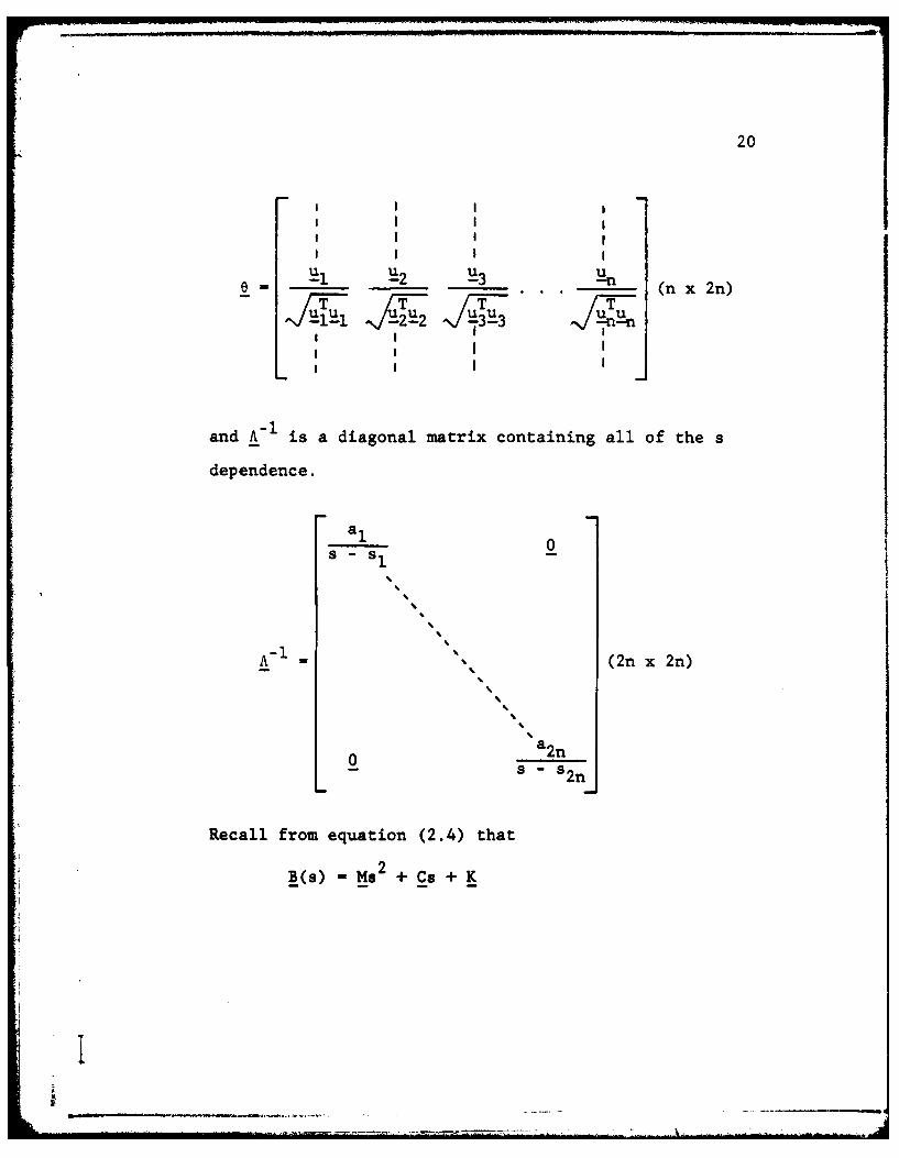
H(s) - e AleT (2.10)

which is an n x n matrix where the columns of e com-

prise the uk modal vectors

IIII

20

al 112 a3 . . Rn (n x2n)

and A- is a diagonal matrix containing all of the s

dependence.

a 10

a-1 (2n x 2n)

Recall from equation (2.4) that

-M2B(s) Ms + CS+ K

21

and evaluate B(s) at s 0 0, then

K - B(O) - _O

One can see that H(O) can be obtained by setting

s = 0 inA-

K - H(O) . (B_ A(O)I eT) -1 (2.21)

Thus the stiffness matrix can be derived from the mea-

sured modal vectors ik and the identified ak and sk

complex scalers.

Recall also that since H equals B-1 ,

H B = I (2.22)

Differentiating (2.22) with respect to s givesI I

HB + H B = 0 (2.23)

and differentiating a second time gives

HB + 2H B + H B 0 (2.24)

* where the prime denotes differentiation with respect

to s. If we then differentiate equation (2.4) with

1 respect to s we obtain

B - 2Ms + C (2.25)

II

22

which when evaluated at s = 0 yields the damping

matrix.

C - B (0) (2.26)

Rearranging equation (2.23) gives

B = -H'1HIB

orI 1

B =-BHB

which when evaluated at s - 0 yields the damping

matrix.I I

C - -B(0) I (0) B(O) - -K H (0) K

or

C -- K [2e(A1 I)'(O)e2] K (2.27)

Differentiating equation (2.25) with respect to s gives

M--,B (2.28)

Rearranging equation (2.24) yields

B -2 H-HB - HIH"B (2.29)

Using the relation B - 1 and evaluating B at s - 0

11

I23

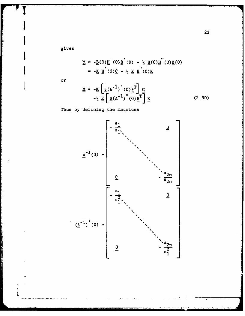
Igives

M - -B(0)H (0)B (0) - B(0)H(0)B(0)

-K H' (0)C - K H (0)K

or

M~~K[e(I(1)(O)eT1

- K[O(A-1) (o)eT] K (2.30)

Thus by defining the matrices

A 1 (0) = .4%*4.

.4.4

'.4.4

.4

52n

a10

5.41~.4

.4

'.44.

.4.4

.4.4

(A1)(0)= .4

.4.4

.4

0 '82n

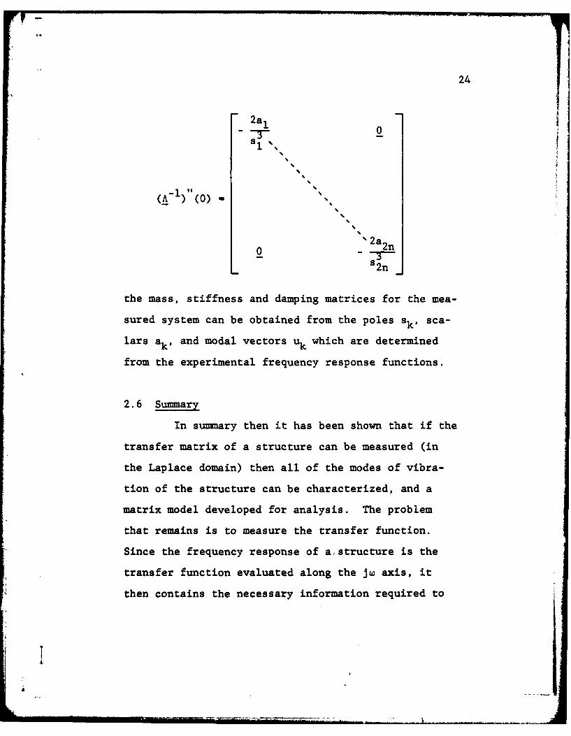
24

2a,0

%

(0) -

0 "2a 2n

L '2n

the mass, stiffness and damping matrices for the mea-

sured system can be obtained from the poles sk s sca-

lars ak, and modal vectors uk which are determined

from the experimental frequency response functions.

2.6 Summary

In summnary then it has been shown that if the

transfer matrix of a structure can be measured (in

the Laplace domain) then all of the modes of vibra-

tion of the structure can be characterized, and a

matrix model developed for analysis. The problem

that remains is to measure the transfer function.

Since the frequency response of a, structure is the

transfer function evaluated along the jw axis, it

then contains the necessary information required to

I..

25

model the transfer function (or matrix). In practice

then, the frequency response functions are measured

and then curve fitting is performed on the data to

curve fit into the s-plane transfer matrix. Chapter

III will discuss some of the different curve fitting

methods.

I

'J 1~

CHAPTER III

MODAL PARAMETER ESTIMATION TECHNIQUES

3.1 Parameter Identification

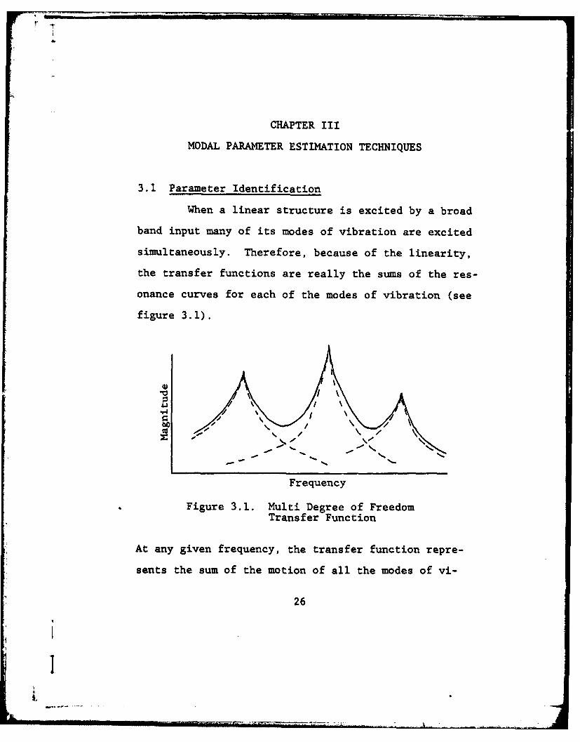
When a linear structure is excited by a broad

band input many of its modes of vibration are excited

simultaneously. Therefore, because of the linearity,

the transfer functions are really the sums of the res-

onance curves for each of the modes of vibration (see

figure 3.1).

44

0 /

Frequency

Figure 3.1. Multi Degree of FreedomTransfer Function

At any given frequency, the transfer function repre-

sents the sum of the motion of all the modes of vi-

26

i 1I

...I-.. . , . . ........ .

27

bration which have been excited. The dashed lines in

Figure 3.1 represent a number of single degree of

freedom modes which when added together form the multi

degree of freedom transfer function. The degree of

overlap (modal overlap) is governed by the amount of

damping of the modes and their frequency separation.

This modal overlap is caused by the contribution of

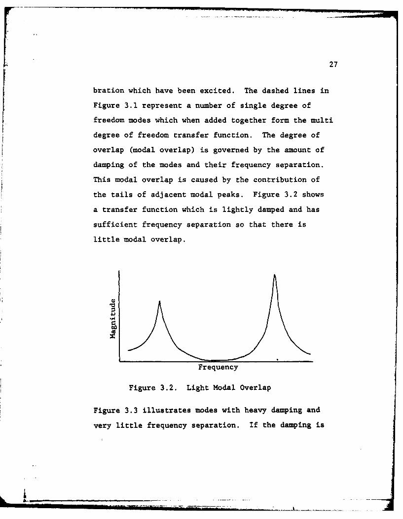
the tails of adjacent modal peaks. Figure 3.2 shows

a transfer function which is lightly damped and has

sufficient frequency separation so that there is

little modal overlap.

Frequency

Figure 3.2. Light Modal Overlap

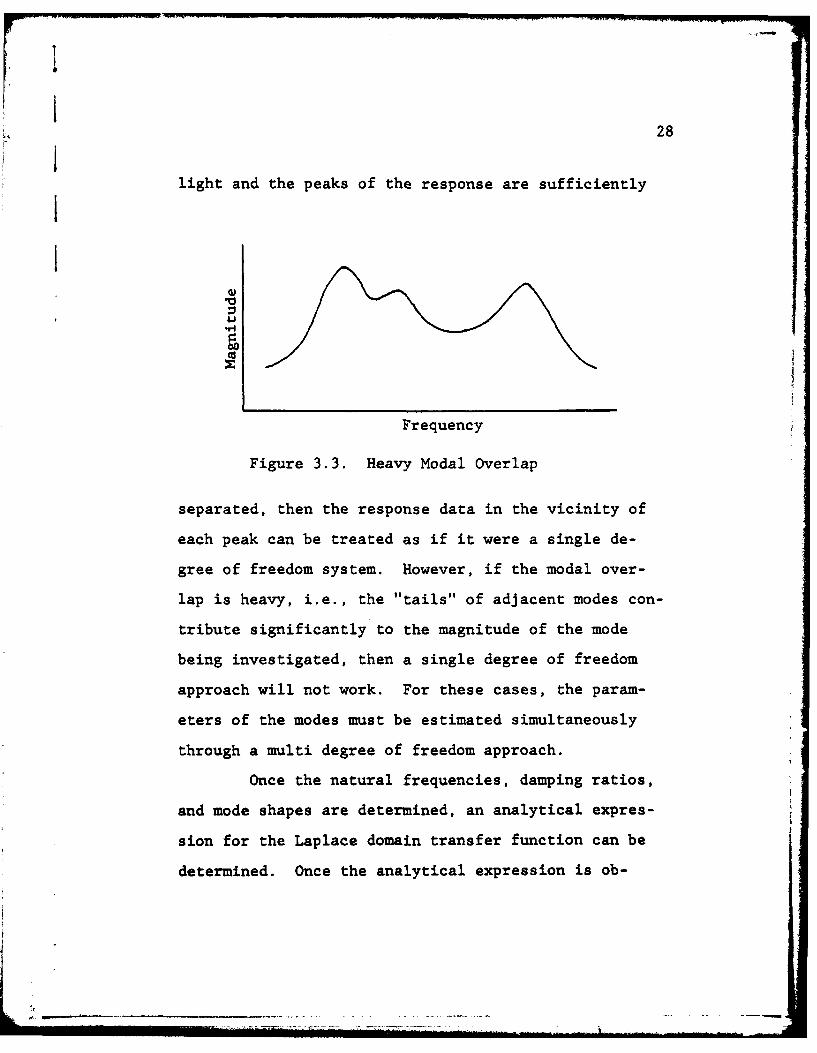
Figure 3.3 illustrates modes with heavy damping and

very little frequency separation. If the damping is

i

I 28

light and the peaks of the response are sufficiently

Frequency

Figure 3.3. Heavy Modal Overlap

separated, then the response data in the vicinity of

each peak can be treated as if it were a single de-

gree of freedom system. However, if the modal over-

lap is heavy, i.e., the "tails" of adjacent modes con-

tribute significantly to the magnitude of the mode

being investigated, then a single degree of freedom

approach will not work. For these cases, the param-

eters of the modes must be estimated simultaneously

through a multi degree of freedom approach.

Once the natural frequencies, damping ratios,

and mode shapes are determined, an analytical expres-

sion for the Laplace domain transfer function can be

determined. Once the analytical expression is ob-

29

tained, it can be used to predict the response of the

system to a particular type of input.

3.2 Single Degree of Freedom Techniques

If the frequency response data exhibits light

damping and the peaks are separated sufficiently so

that very little modal overlap is present then the

following techniques may be considered.

3.2.1 Quadrature Response Technique

Recall that the transfer function of a linear

system for a single mode k can be written as

ak + akhk(s) = + ak (3.1)

s - sk s - sk

where the ak is the complex residue at the kth pole.

If we let s = jw, the frequency response function can

be written

- ak + ak

jw- sk Jw - s k

- +

jW + o k -jwk jw + ak + jW k

(3.2)

I30i

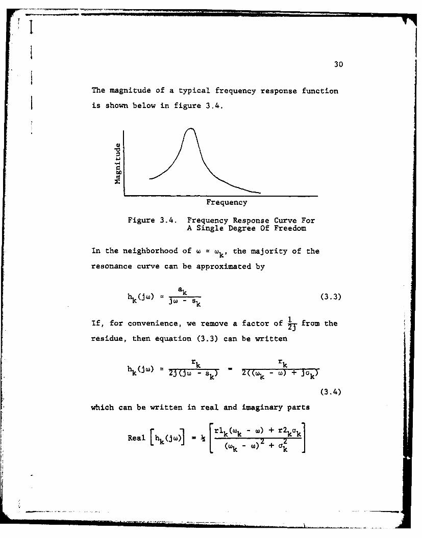
The magnitude of a typical frequency response function

is shown below in figure 3.4.

-r4

Frequency

Figure 3.4. Frequency Response Curve ForA Single Degree Of Freedom

In the neighborhood of w = wk' the majority of the

resonance curve can be approximated by

hk(jw) = j- _ Sk (3.3)

If, for convenience, we remove a factor of . from the

residue, then equation (3.3) can be written

rk rk

k(Jw) =- 2j(j "k) -s 7 2((W " ') + jak)

(3.4)

which can be written in real and imaginary parts

Real rlk( k - w) + r2kak1

[kj~ [rlw)k 2

W)+

(w k--

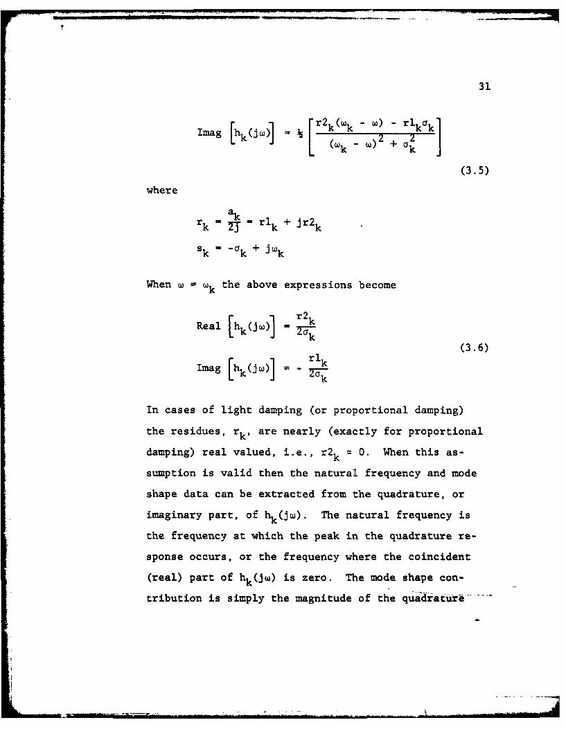
31

Imag [hk~i Q L) r( -W) 2 + U J(k k )

(3.5)

where

rk = k . rlk + jr2 k

Sk = -k + jWk

When w w wk the above expressions become

Real [hk(Jw)] . r2k

(3.6)

Imag [hk(jw)] = - rlk

L i ak

In cases of light damping (or proportional damping)

the residues, rk , are nearly (exactly for proportional

damping) real valued, i.e., r2k = 0. When this as-

sumption is valid then the natural frequency and mode

shape data can be extracted from the quadrature, or

imaginary part, of hk(jw). The natural frequency is

the frequency at which the peak in the quadrature re-

sponse occurs, or the frequency where the coincident

(real) part of hk(Jw) is zero. The mode shape con-

tribution is simply the magnitude of the quadrature

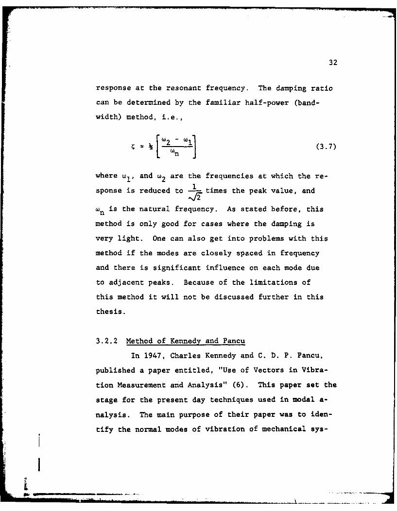
32

response at the resonant frequency. The damping ratio

can be determined by the familiar half-power (band-

width) method, i.e.,

= (3.7)

where wl, and w2 are the frequencies at which the re-

sponse is reduced to - times the peak value, and

On is the natural frequency. As stated before, this

method is only good for cases where the damping is

very light. One can also get into problems with this

method if the modes are closely spaced in frequency

and there is significant influence on each mode due

to adjacent peaks. Because of the limitations of

this method it will not be discussed further in this

thesis.

3.2.2 Method of Kennedy and Pancu

In 1947, Charles Kennedy and C. D. P. Pancu,

published a paper entitled, "Use of Vectors in Vibra-

tion Measurement and Analysis" (6). This paper set the

stage for the present day techniques used in modal a-

nalysis. The main purpose of their paper was to iden-

tify the normal modes of vibration of mechanical sys-

I

£ii .. .'" ........ . . ... ." - ' ......... ... .......-...... .. ... .. ........

33

tems. They assumed that the damping in the system was

proportional to the displacement and 900 out of phase

with it. They also assumed that the off-resonant vi-

bration is constant in phase and magnitude as the sys-

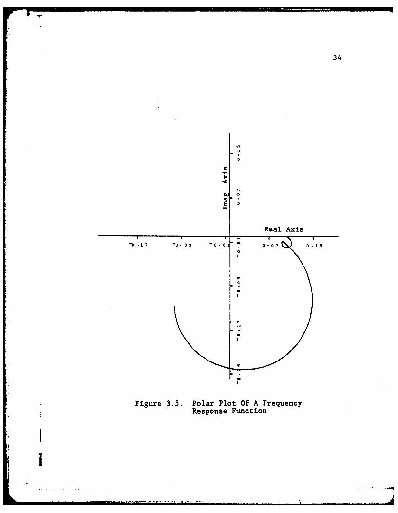
tem passed through a resonance. The authors made use

of a vector response plot, more commonly called a

polar plot or Nyquist plot, which plotted both real

and imaginary components of the frequency response

data vs. frequency. An example of a Nyquist plot is

illustrated in Figure 3.5. Their basis for using this

type of plot was that near a resonant frequency, the

polar plot would describe a circular arc. The plot

for a single degree of freedom system is shown in

Figure 3.6. In terms of the analytical transfer func-

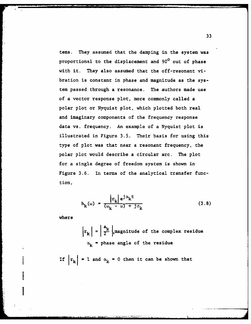
tion,

Irki ej akthk() = (Wk - W) (3.8)

where

rk = -- J magnitude of the complex residue

a = phase angle of the residue

If Irki - 1 and ak - 0 then it can be shown that

II

34

b~o

Real Axis

-0 .1 7 -0. 09 -00 1 0 -0 7 0.-15S

Figur 3.5 Polr Plt OfA Frqec

Respose Fuctio

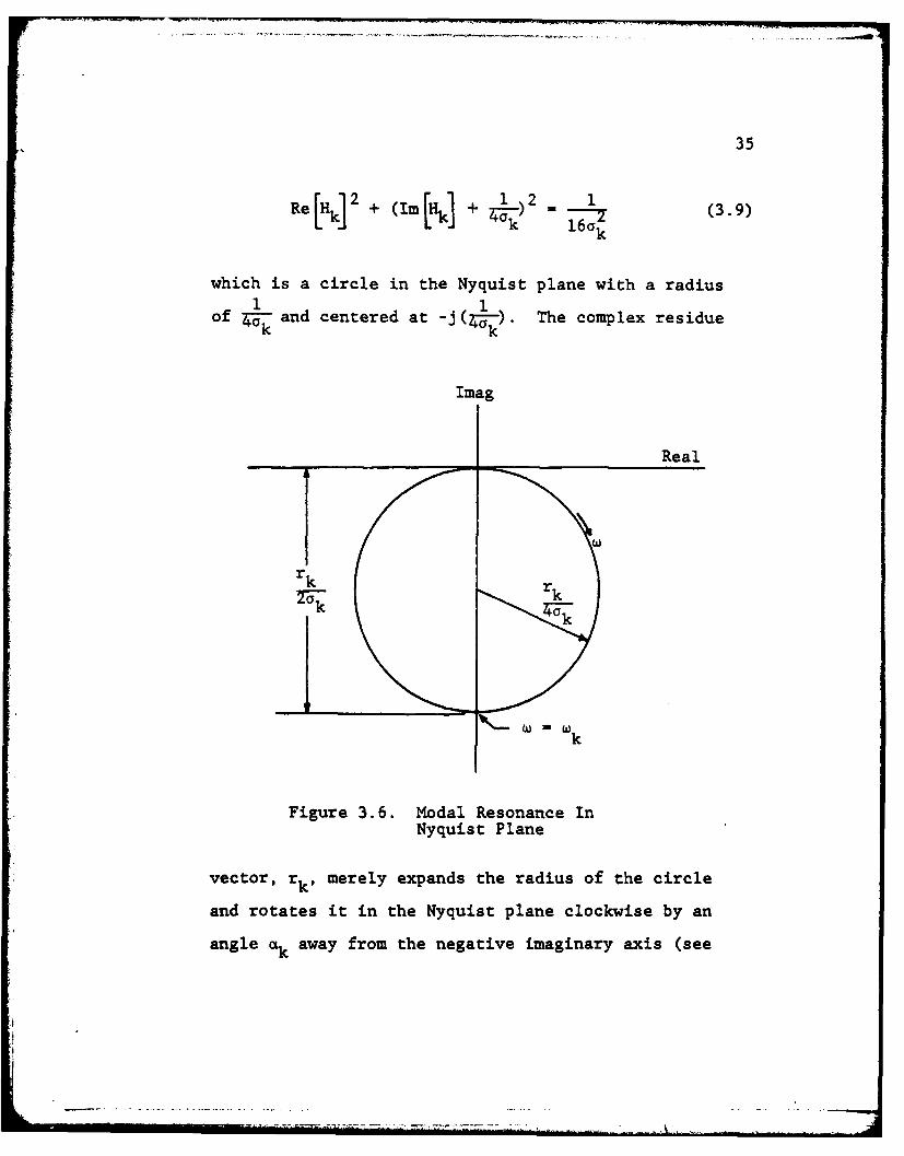
35

Re [Hk] 2 + (Im[Hk] + 1 2 1 (3.9)L.I k) -l6 ak

which is a circle in the Nyquist plane with a radius11

of k and centered at -j ( -). The complex residuek k

Imag

Real

rk rk

k

Figure 3.6. Modal Resonance InNyquist Plane

vector, rk, merely expands the radius of the circle

and rotates it in the Nyquist plane clockwise by an

angle ak away from the negative imaginary axis (see

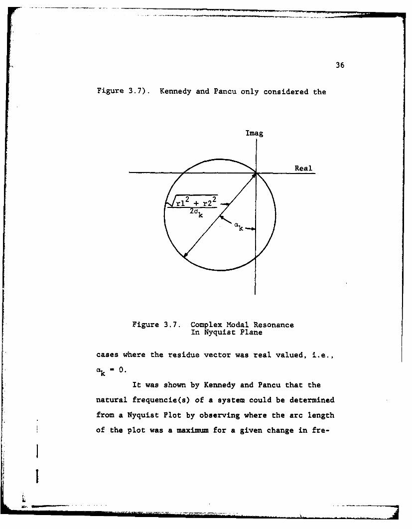
36

Figure 3.7). Kennedy and Pancu only considered the

Imag

Real

rl 2 + r2 2

2a k

Figure 3.7. Complex Modal ResonanceIn Nyquist Plane

cases where the residue vector was real valued, i.e.,

cak - 0.

It was shown by Kennedy and Pancu that the

natural frequencie(s) of a system could be determined

from a Nyquist Plot by observing where the arc length

of the plot was a maximum for a given change in fre-

AIS..

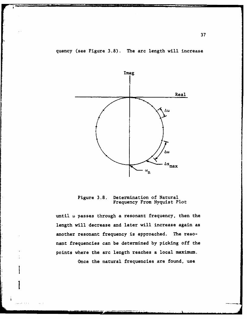
37

quency (see Figure 3.8). The arc length will increase

Imag

Real

As

__A - Smax

n

Figure 3.8. Determination of NaturalFrequency From Nyquist Plot

until w passes through a resonant frequency, then the

length will decrease and later will increase again as

another resonant frequency is approached. The reso-

nant frequencies can be determined by picking off the

points where the arc length reaches a local maximum.

Once the natural frequencies are found, use

1

38

is made of the fact that near a resonance the arc ap-

proximately describes a circle. A circle is then fit

to the data near each resonant frequency.

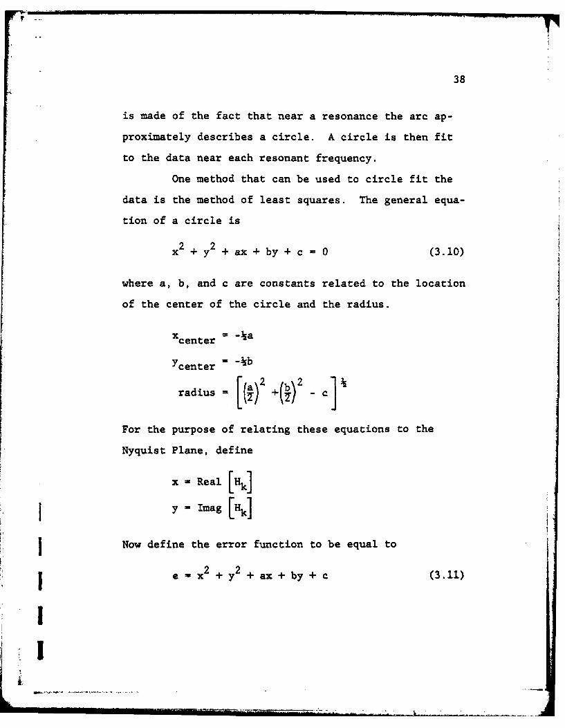
One method that can be used to circle fit the

data is the method of least squares. The general equa-

tion of a circle is

X + y + ax + by + c = 0 (3.10)

where a, b, and c are constants related to the location

of the center of the circle and the radius.

Xcenter m -ka

Ycenter - -kb

radius - () +(.) -

For the purpose of relating these equations to the

Nyquist Plane, define

x s Real [Hk]

I y -Imag [Hk]

I Now define the error function to be equal to

S-x 2 + y2 + ax + by + c (3.11)

Ii!

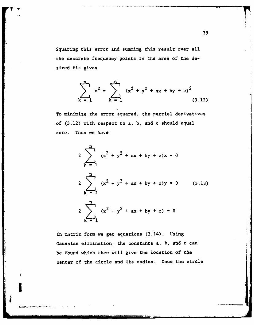
39

Squaring this error and summing this result over all

the descrete frequency points in the area of the de-

sired fit gives

= Z (x+ + ax + by + c)2

k- i k- 1 (3.12)

To minimize the error squared, the partial derivatives

of (3.12) with respect to a, b, and c should equal

zero. Thus we have

n

2 (x 2 + y2 + ax + by + c)x 0

n

2 1 ( x2 + y2 + ax + by + c)y - 0 (3.13)

n

2 1 (x2 + y2 + ax + by + c) = 0

k-i

In matrix form we get equations (3.14). Using

Gaussian elimination, the constants a, b, and c can

be found which then will give the location of the

center of the circle and its radius. Once the circle

iA

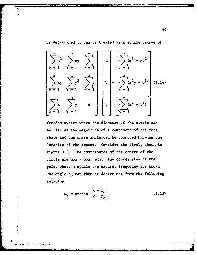
40

is determined it can be treated as a single degree of

n n n n

>x2 >xy x a _ xl+ xy2

k-i k=l - k-i

n n n n

y y y b - Z x2y + y3) (3.14)

n n n

k-iZY k-i

freedom system where the diameter of the circle can

be used as the magnitude of a component of the mode

shape and the phase angle can be computed knowing the

location of the center. Consider the circle shown in

Figure 3.9. The coordinates of the center of the

circle are now known. Also, the coordinates of the

point where w equals the natural frequency are known.

The angle ak can then be determined from the following

relation

a arctan - (3.15)

I

j

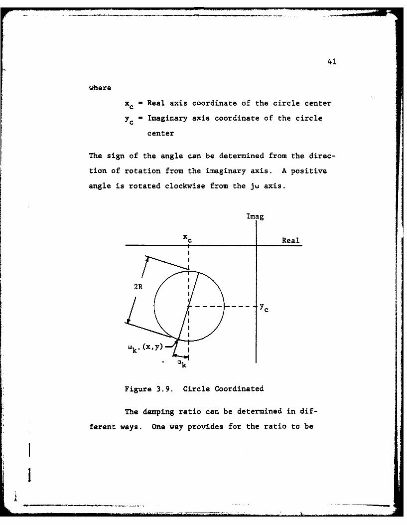
41

where

xc - Real axis coordinate of the circle center

Yc = Imaginary axis coordinate of the circle

center

The sign of the angle can be determined from the direc-

tion of rotation from the imaginary axis. A positive

angle is rotated clockwise from the jw axis.

Imag

xc Real

I1

2R

C

k'(x, y)--

lk

Figure 3.9. Circle Coordinated

The damping ratio can be determined in dif-

ferent ways. One way provides for the ratio to be

1

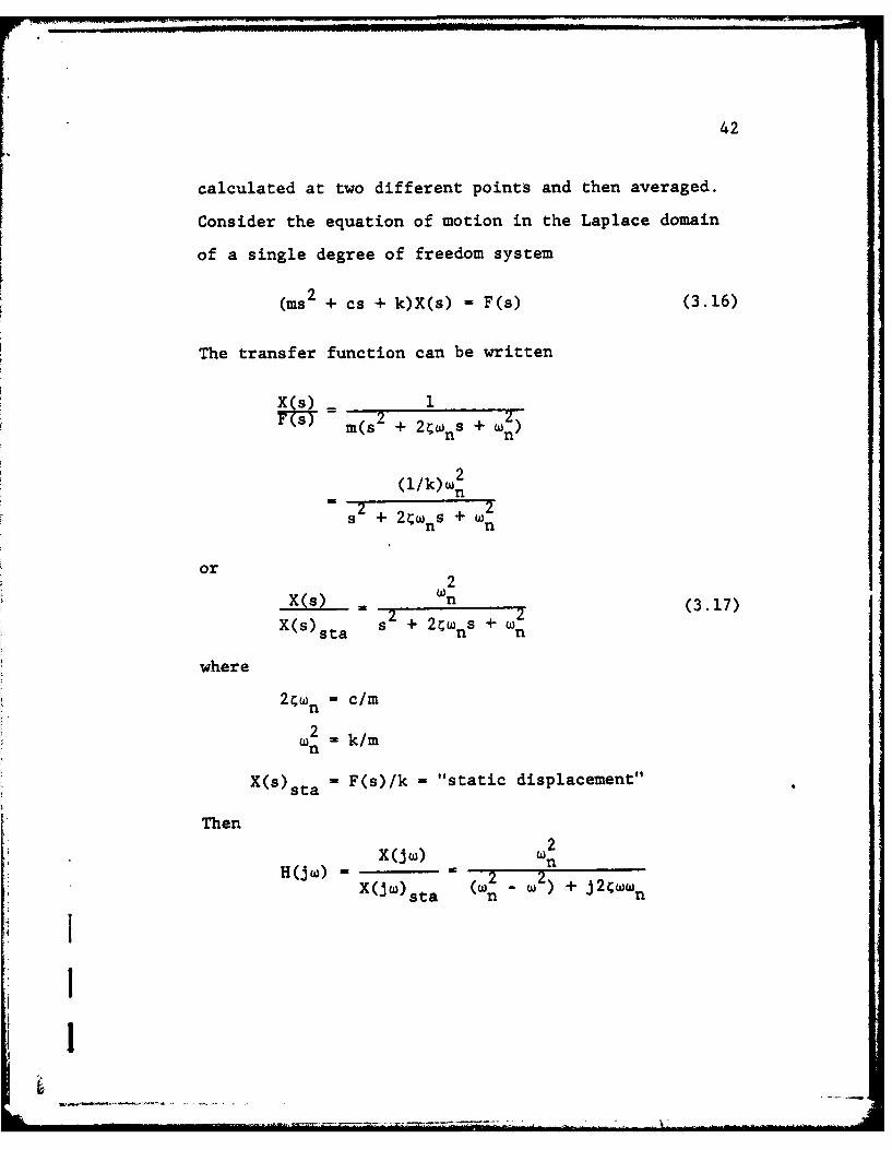
42

calculated at two different points and then averaged.

Consider the equation of motion in the Laplace domain

of a single degree of freedom system

(ms2 + cs + k)X(s) = F(s) (3.16)

The transfer function can be written

in) (s 2+ 2ws + wn n-- 2

(1/k)w2

n2 2s + 2CwnS +wn n

orW2

X(S) n _____2s _ + 2(3.17)X()sta s + 2w s + wsan n

where

2C n = c/m

n 2 .k/m

X(S)sta = F(s)/k = "static displacement"

Then

X(jW) W 2

2 2X(jw)st (Wn W w + j2CwwnX( sta (n "

1I

I43I

2

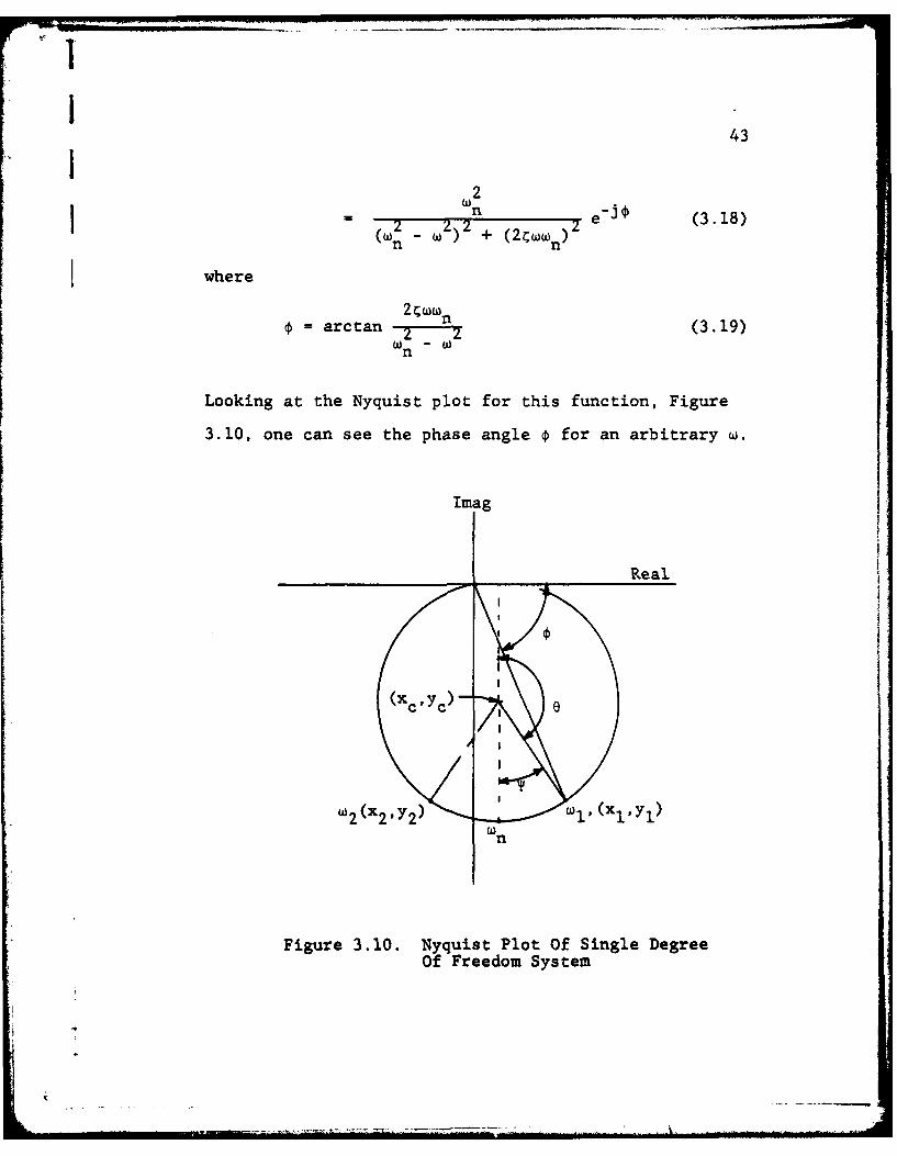
) -2 + e (3.18)n n

where

= arctan 2 "WW (3.19)Wn - W

Looking at the Nyquist plot for this function, Figure

3.10, one can see the phase angle 0 for an arbitrary w.

Imag

Real

f

(xyC)- -l(

w2 (x23y 2) vYl )

wn

Figure 3.10. Nyquist Plot Of Single DegreeOf Freedom System

44

Now define e = 20 where 6 is measured from the diam-

eter of the circle drawn through the resonant fre-

quency. Substituting e - 20 into equation (3.19) and

solving for c gives

(n 2- w2) tan (8/2)= 2Wn (3.20)

The only information needed to get the angle 8 are the

coordinates of the center of the circle and the coor-

dinates of a frequency point on one side or the other

of the resonant frequency. Consider the example shown

in Figure 3.10.

T = arctan

I y1 - Y

6 = 1800 - T

Substituting into equation (3.20) gives

2( - 2 tan 180 -

The same thing can be done using w2 and then the two

values of C averaged.

This method of circle fitting is accomplished

for each resonant frequency observed in the Nyquist

i

45

plot for a given frequency response. If this is accom-

plished for each frequency response in one row or col-

umn of the transfer matrix, then the mode shapes can

be determined, i.e.

Mode 1=I(ap2l (al)21}

where

(a,),1 = diameter of circle at wI determined

from frequency response h1l

(a1)21 = diameter of circle at w, determined

from frequency response h21

and similarly for the phase angles (ak)ij.

Immediately one can see a problem with this

type of approach. If the modes happen to be closely

coupled where one mode dominates, the circle fit of

the smaller mode may not have sufficient points to

resolve the amplitude of the residue, i.e., the di-

ameter of the circle fit through the smaller mode may

be incorrect thus giving rise to errors in the mode

shape and also the damping ratio associated with that

mode.

46

In order to reduce the limitations imposed by

single degree of freedom assumptions, one must consid-

er a multi-degree of freedom curve fit, which is the

subject of Section 3.3.

Chapter IV will present example problems

using this method of determining modal parameters.

Also, Appendix A gives a listing of a computer al-

gorithm derived for circle fitting frequency response

data.

3.3 Multi Degree of Freedom Curve Fitting

For cases where the amount of modal overlap

is sufficient to cause significant errors by use of

single degree of freedom techniques, a multi degree

of freedom technique must be used. Two techniques

will be described in this section.

3.3.1 Complex Curve Fit

This technique is one which matches the sum-

mation

n

h(s) -'l [-k + I (3.21)- sk s - sk

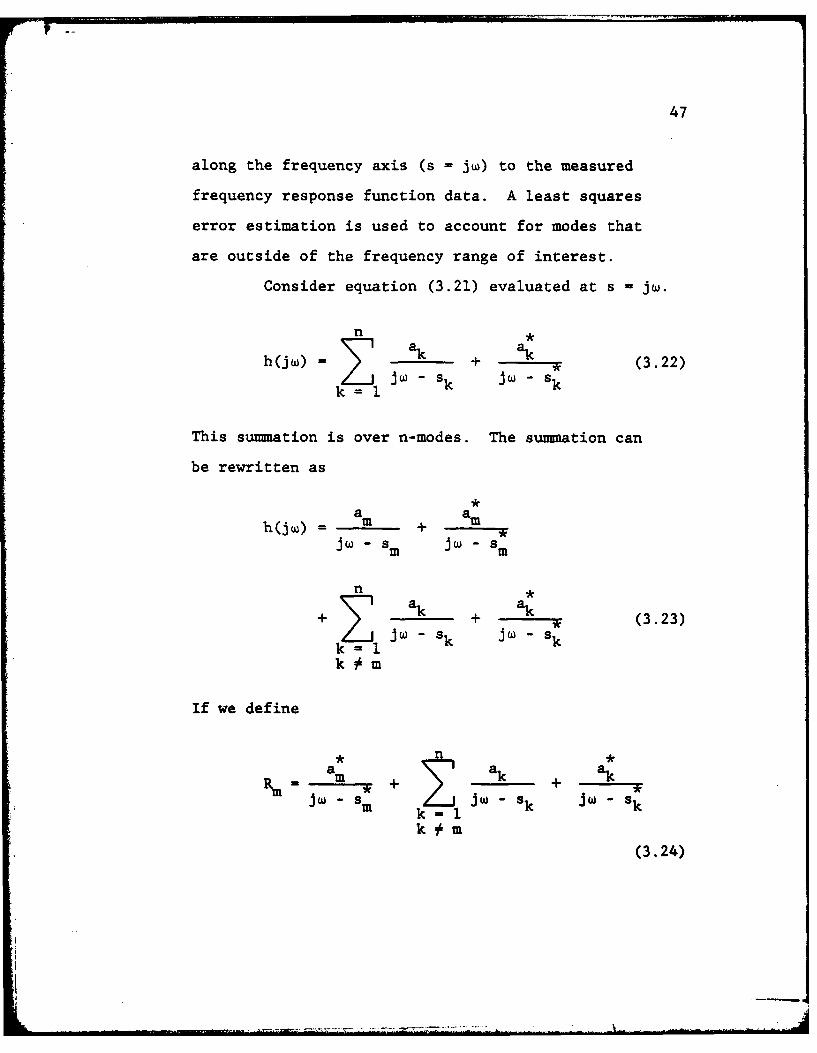
47

along the frequency axis (s = jw) to the measured

frequency response function data. A least squares

error estimation is used to account for modes that

are outside of the frequency range of interest.

Consider equation (3.21) evaluated at s = jW.

n *

h(jw)- 7 ak + ak s (3.22)

k = I - k J- k

This summation is over n-modes. The summation can

be rewritten as

a amh(jw) m +jW - s m JW - sm

n m

+ a k + a (3.23)jw - sk jW - skk 0 mk~m

If we define

. n

Rm - Zm -k + -kk~ak

k m

(3.24)

JI. . .. . ... ..... . - - '-------,'r. _ z - " , - -- T;. .. , . . ,

48

then equation (3.23) can be written

ah~jw) jW - m + R

m

am + m (3.25)am + i ( W "- Wm)

If the system is lightly damped, i.e., am is small, it

is noted that in the neighborhood of w = wmS the first

term in equation (3.25) dominates, and Rm is nearly

constant for small changes in w. Using this assump-

tion, consider the mth peak in the magnitude curve of

h(jw) (see Figure 3.11). Pick two points on the curve,

one on each side of the peak. Now then, evaluate

03 Ihih 21

Wi w2 Frequency

Figure 3.11. Two Point Estimation

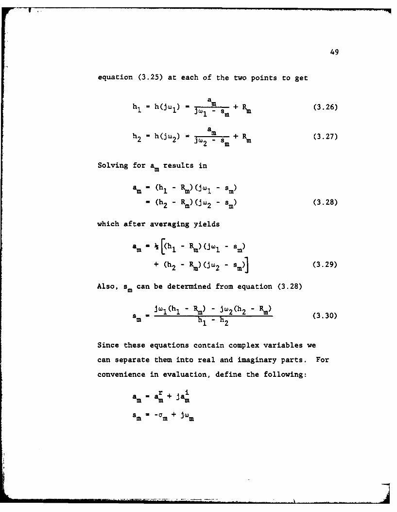
49

equation (3.25) at each of the two points to get

amh- h(jw i ) = jw1 _Sm +m (3.26)

ah2 = h(jw 2) = jW2 "m +m (3.27)

Solving for am results in

am- (h- - Re)(jwl - si)

= (h2 - R%)(jw 2 - sm ) (3.28)

which after averaging yields

am = 4[(h - Rs)(w - )

+ (h2 - Rm)(jw 2 - si)] (3.29)

Also, sm can be determined from equation (3.28)

jwl(h1 - Rm) - jw2 (h2 - R)sm - hl - h2 (3.30)

Since these equations contain complex variables we

can separate them into real and imaginary parts. For

convenience in evaluation, define the following:

am - am + Jam

Sm = "_rn + J m

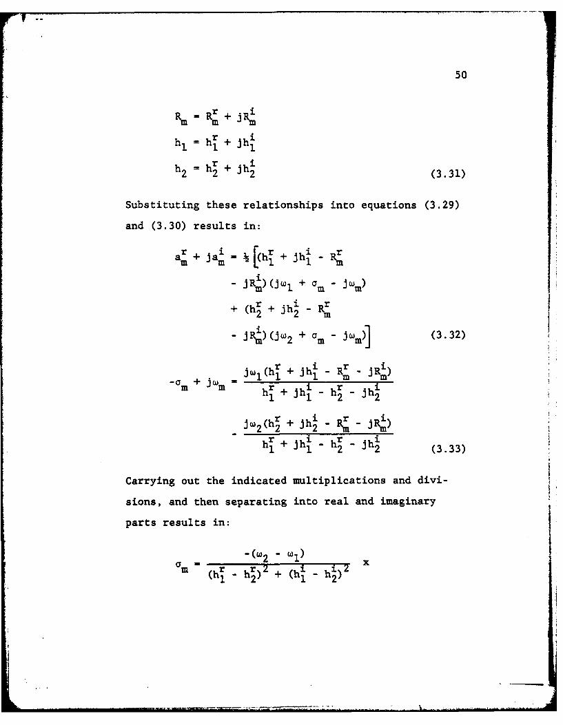
50

R. Rr +jRiR m m

h= h + jhi

= h2 + jh2 (3.31)

Substituting these relationships into equations (3.29)

and (3.30) results in:

ar Iam + jam -k [(h 1+ ihi R

- jR;)(jwl + am "jm)

r i Rr

+ (h2 + jh 2 -

- jR)(Jwi2 + am jw~ (3.32)mm m+ -

jwl(h r + ihi Rr - iJi

.. +ow - R-m +Jm " r I h r 3.

rr

h I + jh - h2 - (333)

Carrying out the indicated multiplications and divi-

sions, and then separating into real and imaginary

parts results in:

a -(w2 - wl) x(hi h2) + (h1 - h2)

-- ---- -- -

II

Imh

I 51

Rm(hl h')- R(h h h)

1 l2 1 (22

+ h h i - hr] (3.34)

m r[ r 2 i 71 )

m (h1 h 2 - h2)

r 3. ) [hrh r 1) + R a(h' hsee

thatIN wl 1n 2m ca efudi m 1 2)]n ec

+ (hr)2 _ hrh r + (h1r)2]

+ ha) h2 _ hhe + (hc o )2] (3.35)

am k[am(h14 + hr 2R )

i i i

+ wm(hi + h2 2R M) - W 1(h, R.)

- w(h' R) (3.36)

am [am (h' + h' 2R )

-wm(h r + h r-2R ) + w(hr-_Rr)

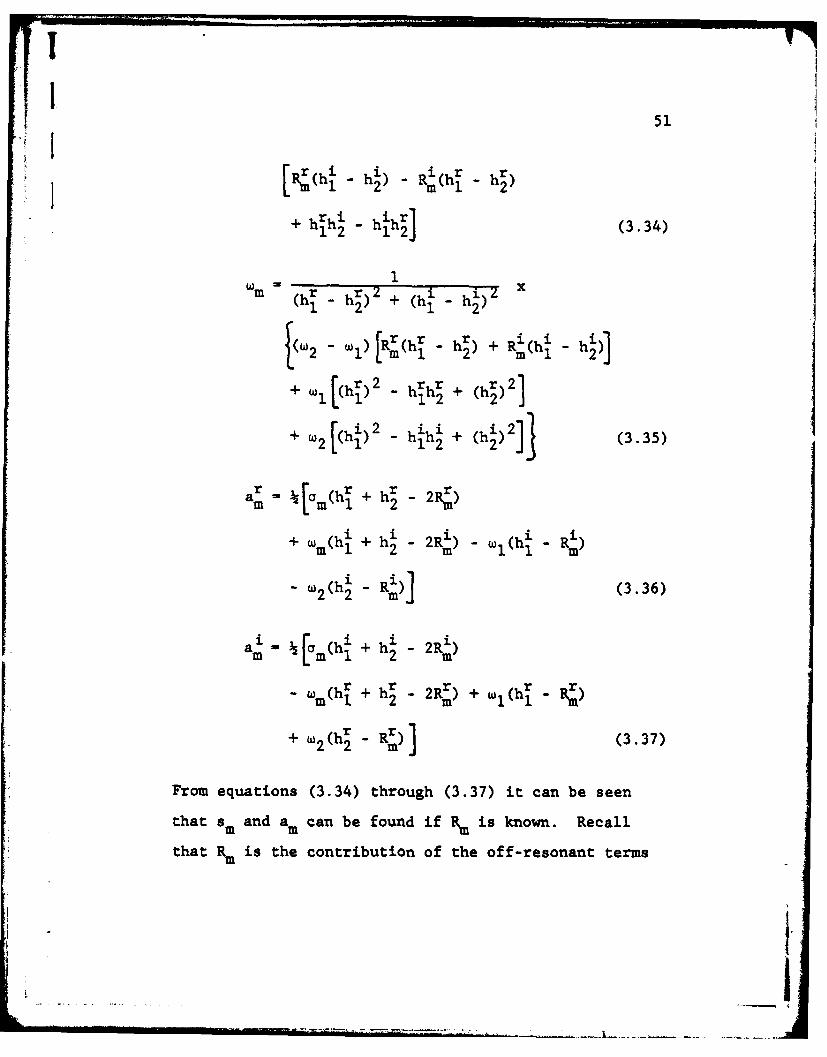
+ W 2(h - R )] (3.37)

From equations (3.34) through (3.37) it can be seen

that smand am can be found if Rm is known. Recall

that Rn is the contribution of the off-resonant terms

52

(equation (3.24)). If an estimate is made for Rm

then values for sm and am could be obtained and then

an iterative technique could be established to im-

prove the estimates.

The technique used in this paper is to as-

sume Rm is initially zero and then solve for sm and

am. Then using these values, substitute into equa-

tion (3.24) and solve for a new Rm. This technique

works fine when all of the modes are present in the

frequency range of analysis and modal overlap is

light. However, in real structures there are an in-

finite number of modes, all of which cannot be mea-

sured. Therefore it may be necessary to consider a

contribution to the transfer functions due to modes

with natural frequencies outside of the frequency

range of analysis. This contribution can be con-

sidered either to be a complex constant or a complex

function of frequency. For the purpose of simplicity,

we will consider only the case where it is a complex

constant.

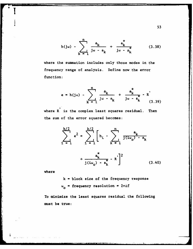
The constant can be determined by a least

squares fit to the following:

53

n *- + k (3.38)

h(jw) a

jw - sk JW - Sk

where the summation includes only those modes in the

frequency range of analysis. Define now the error

function:

n *

e = h(jw) - k + k R

= k (3.39)

where R is the complex least squares residual. Then

the sum of the error squared becomes:

2 a22 ke i -j(iwo 0 S k

+ ak ,R 2+ - R]

j(iw) - sk (3.40)

where

k - block size of the frequency response

-e " frequency resolution - 2wAf

To minimize the least squares residual the following

must be true:

54

k/2 n

Z-hi J (io). skik~l

+ a k (k/2)j (i,,0) - Sk.j (3.41)

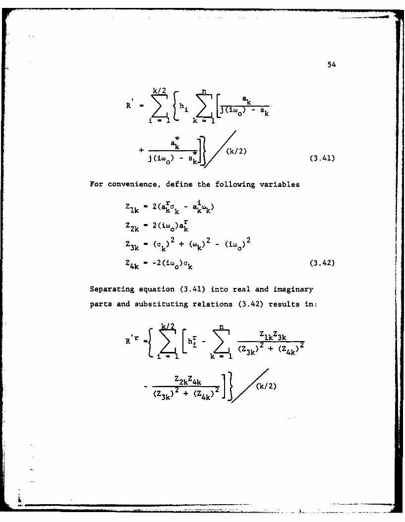
For convenience, define the following variables

Zlk '2( k 2 ri

Z2k = 2(iw )ar

Z3k ' ('k) 2 + (wk) 2 (iWo)2

Z4k - -2 (iw o)ak (3.42)

Separating equation (3.41) into real and imaginary

parts and substituting relations (3.42) results in:

~kL2 nR'r T r Zlk Z3k

Rr hi - (Z3k) + (Z4k)

Z2kZ4k 2 I(2)(Z3k)2 + (Z4k)2

I>.

55

k/2 n Z2kZ3k

k (Z3k) + (Z4k)2

ZlkZ4k (k/ 2

2 22)(Z3k) + (Z4k)

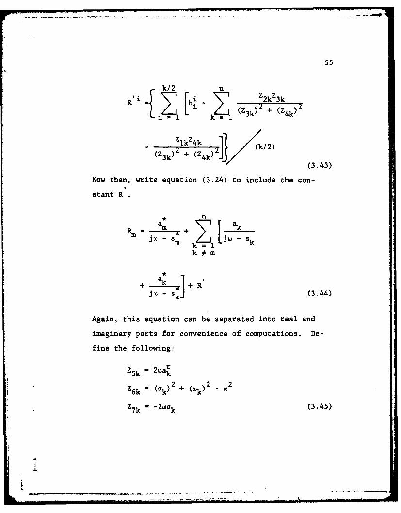
(3.43)

Now then, write equation (3.24) to include the con-

stant R

a a- + k

j - s j sk-ik m

+ a +RjW - sk I (3.44)

Again, this equation can be separated into real and

imaginary parts for convenience of computations. De-

fine the following:

Z5k k 2wa

Z6k ( (k) + (wk) 2

Z7k - -2 wak (3.45)

I7

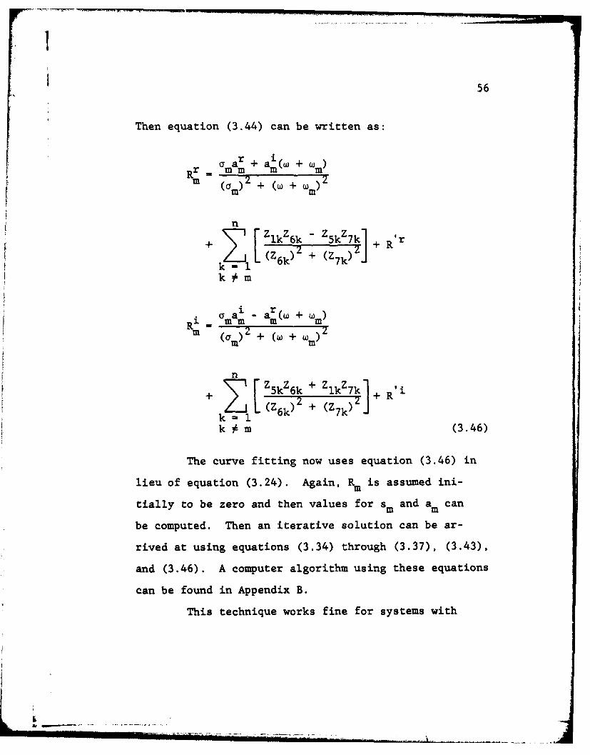
56

Then equation (3.44) can be written as:

Rra= mar + al(W + W)

(a mr)2 + +m2

nZ -

Ik6k 5kZ7r+2 2 +R r

1 (1 6k) + (Z) 07k#m

o a 1 ar (w+

Ri a m m m ( m )

m (m) 2 + (Z+ )

n2

k1 Z6 k) + (Z7k)Y

k #m (3.46)

The curve fitting now uses equation (3.46) in

lieu of equation (3.24). Again, Rm is assumed ini-

tially to be zero and then values for sm and am can

be computed. Then an iterative solution can be ar-

rived at using equations (3.34) through (3.37), (3.43),

and (3.46). A computer algorithm using these equations

can be found in Appendix B.

This technique works fine for systems with

a.L *

57

light to moderate damping. When there is heavy modal

overlap due to closely spaced resonant frequencies,

but with light damping, the technique again works rea-

sonably well. However if there are closely spaced

frequencies and the damping ratios approach 0.2, then

the error in the estimated parameters begins to get

too large. A discussion on the error versus damping

ratio is presented in Chapter IV in conjunction with

the example problems.

3.3.2 Curve Fitting of Quadrature Response

As previously mentioned, the total response

curve fitting technique works well when the degree of

modal overlap is light. As the degree of overlap in-

creases, this method yields greater errors. One meth-

od which provides more accurate results is to curve

fit the quadrature, or imaginary, part of the transfer

function. The main reason for choosing the quadrature

response is the rapid change it displays near resonant

frequencies. The quadrature response peaks much

sharper at a resonance as compared to the total re-

sponse curve.

In this section, the imaginary curve fit algo-

rithm will be developed. The assumptions used appear

58

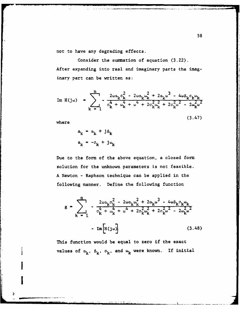
not to have any degrading effects.

Consider the summation of equation (3.22).

After expanding into real and imaginary parts the imag-

inary part can be written as:

n 2w a 2 _ w w 2 + 2 3 _ w a W

Im H(jW) = k " 2 + 2 k k kk 2Z =- a4 + W + W4 + 2azw + 2a 2 - 2w 2

k =l1 k +2 k k k 2 kw

(3.47)where

ak = ak + Jak

S k = - k + J k

Due to the form of the above equation, a closed form

solution for the unknown parameters is not feasible.

A Newton - Raphson technique can be applied in the

following manner. Define the following function

n ~ 2 a - 2wckw 2 + 2 atkW3 _ 4w$k akWk

Z = a4 + W + W4 + 2a 1 + 2aow 2 - 2w 2 2g k - k k 22 22 22k

- Im[H(ji (3.48)

This function would be equal to zero if the exact

values of akf ak' ak, and wk were known. If initial

I

59

estimates were available for these parameters then an

iterative technique could be applied to improve the

estimates. It can be seen from equation (3.47) that

if the parameters ak and wk are known then equation

(3.47) becomes a linear function of ak and 8k , i.e.,

the residues (ak). Thus, it would only be necessary

to provide initial estimates for natural frequencies

and damping ratios. The estimates for the residues

(ak) are then obtained by using a Gaussian elimination

technique on equation (3.47) evaluated at 2n frequency

points (preferably two points on each peak).

In order to define an iterative technique for

the solution of equation (3.47), the function g (equa-

tion (3.48)) can be rewritten as

g = f(am' 4mP am) am) + f (ak, wk' ak' 8k) - hi

(3.49)

where

f(amp Wmy am' am) = the term of equation

(3.48) associated with the

mth pole

f (ak' Wkv ak k) = the summation of all terms

in equation (3.48) except

for the term associated

with the mth pole

-I

60

hi Im [h(QjJ]

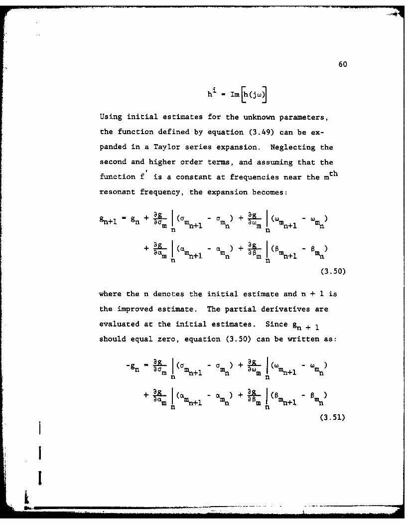
Using initial estimates for the unknown parameters,

the function defined by equation (3.49) can be ex-

panded in a Taylor series expansion. Neglecting the

second and higher order terms, and assuming that the

function f' is a constant at frequencies near the mth

resonant frequency, the expansion becomes:

gn+l =n + am (m+l- n m (mn+l "nn n

am I mn+l - %'mn D+ - I (mn+l mnnnn n

(3.50)

where the n denotes the initial estimate and n + 1 is

the improved estimate. The partial derivatives are

evaluated at the initial estimates. Since gn + i

should equal zero, equation (3.50) can be written as:

21- a ) +2-~ (W= -E [(mnl," +mn +lmn-gn = am m Omn) D~m I (mn+l nn n

aam I(mn+l -ran) +Sm I mn+l mn

n n

(3.51)

OII

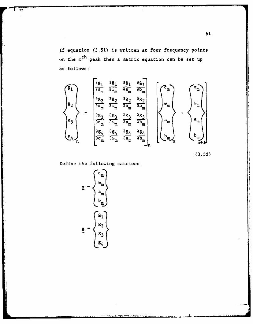
61

If equation (3.51) is written at four frequency points

on the mth peak then a matrix equation can be set up

as follows:

ag1 Dg, ag1 ag1

a92 a92 a92 a92

a93 a93 a93 a93 am a93a-y w Tai WmV i n

a94 a 94 a94 394 b bnn i n D n n+l!

L Jn

(3.52)

Define the following matrices:

Mnj

91

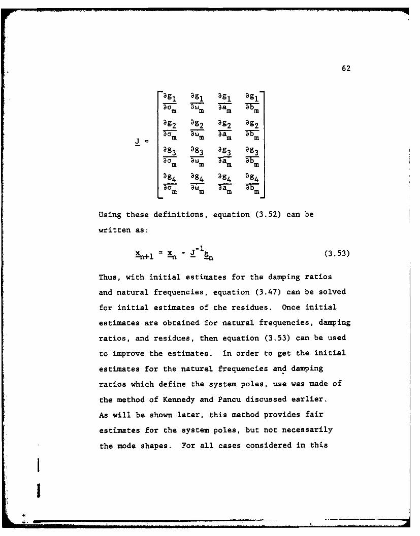
62

agl ag ag1 aglin- i- n in m

a9g2 g2 a9g2 a9g2aaab

3g3 g3 39g3 a9g3

ag4 g4 3g4 a9g4w- Tw- ra- i-

Using these definitions, equation (3.52) can be

written as:

+ x -i (3.53)Enl E -T -g

Thus, with initial estimates for the damping ratios

and natural frequencies, equation (3.47) can be solved

for initial estimates of the residues. Once initial

estimates are obtained for natural frequencies, damping

ratios, and residues, then equation (3.53) can be used

to improve the estimates. In order to get the initial

estimates for the natural frequencies and damping

ratios which define the system poles, use was made of

the method of Kennedy and Pancu discussed earlier.

As will be shown later, this method provides fair

estimates for the system poles, but not necessarily

the mode shapes. For all cases considered in this

Ii

63

thesis, the circle fit method provided estimates with

sufficient accuracy for this algorithm to converge.

The imaginary curve fitting technique provides

very accurate estimates for the modal parameters for

systems with a light degree of modal overlap. As the

degree of modal overlap increases, more accurate ini-

tial estimates are required for this method to con-

verge. As the damping ratio approaches 0.2 with reso-

nant frequencies closely spaced, this method becomes

unstable if the initial estimates for natural fre-

quency and damping ratio are in error by more than

10%.

3.4 Summary

Each of these methods has its advantages and

limitations. Chapter IV will present two example

problems, each one analyzed by each curve fit method

discussed in Sections 3.2.2, 3.3.1, and 3.3.2. the

results are sumarized to show the advantages and

limitations of each method.

b

II

CHAPTER IV

I EXAMPLES OF CURVE FITTING TECHNIQUES

I 4.1 Introduction

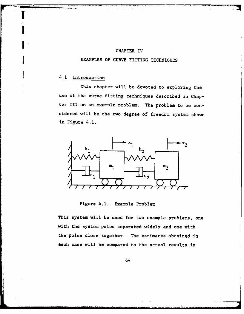
This chapter will be devoted to exploring the

use of the curve fitting techniques described in Chap-

ter III on an example problem. The problem to be con-

sidered will be the two degree of freedom system shown

in Figure 4.1.

k1x1k 2 ,, 2

l l ll1ll2

Figure 4.1. Example Problem

This system will be used for two example problems, one

with the system poles separated widely and one with

the poles close together. The estimates obtained in

each case will be compared to the actual results in

64

65

order to show the usefulness and extent of each curve

fit method.

4.2 Example Problem One

Define the variables of Figure 4.1 as:

Mi M 1 m2 - 6

kI = 100 k2 = 6

c1 M .1 c2 = .1

For this system, the actual values for the modal

parameters as computed via a complex eigen-solver

routine are:

=i - 0.97103 rad/sec 2 f 10.29834 rad/sec

-I - 0.00765 ;2 = 0.00980

0O.05711 /-359.170mode 1 1.0 /00

.0 / 0 0

m.00964 /-171. 27 J

Recall that the transfer matrix can be written as:

&.k-a

66

[hll(s) h12 (s)]

H(s) ILh2l(s) h22 (s)j

If the frequency response functions h1l(jw) and h21(JW)

are measured, then all of the modal parameter estima-

tions may be obtained. In all of the cases to follow,

hll and h21 are used to determine the estimates of the

natural frequencies, damping ratios, and mode shapes.

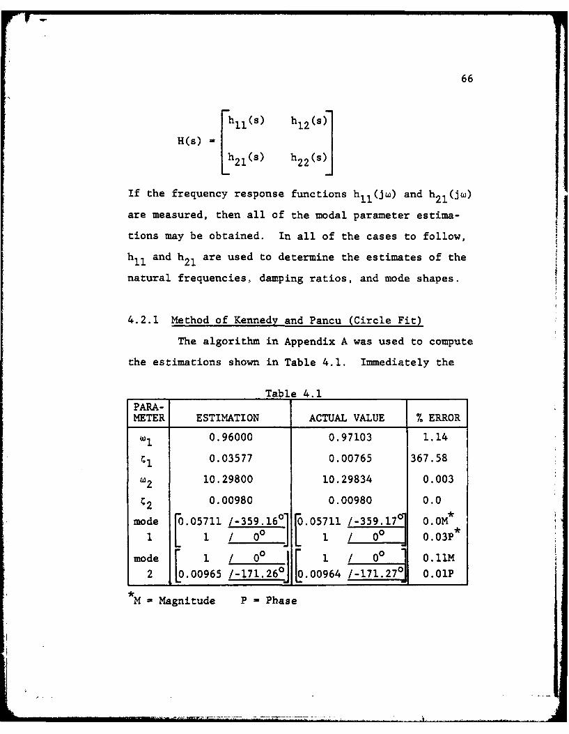
4.2.1 Method of Kennedy and Pancu (Circle Fit)

The algorithm in Appendix A was used to compute

the estimations shown in Table 4.1. Immediately the

Table 4.1

PARA-METER ESTIMATION ACTUAL VALUE % ERROR

(l 0.96000 0.97103 1.14

CI 0.03577 0.00765 367.58

w2 10.29800 10.29834 0.003

0.00980 0.00980 0.0

mode 0.05711 /-359.16 05711 /-359.17 0.OM1 1 00 1 00 0.03P*

mode 1 1 0 F 1 00 0.11M

2 0.00965 /-171.260 0.00964 /-171.270 0.01P

*M - Magnitude P - Phase

67

error for l stands out. This gross error can be

readily explained, and is a good example of one of the

problems associated with this method. This error was

the result of insufficient frequency resolution in the

frequency response data. The above problem was re-

worked with better resolution by looking only at the

frequencies near wI. This provided a 0.01% error in

CI"

One other problem associated with this method

is that of one mode dominating the other nearby modes.

For this problem, even though mode 2 dominates, it is

separated far enough in frequency so as not to inter-

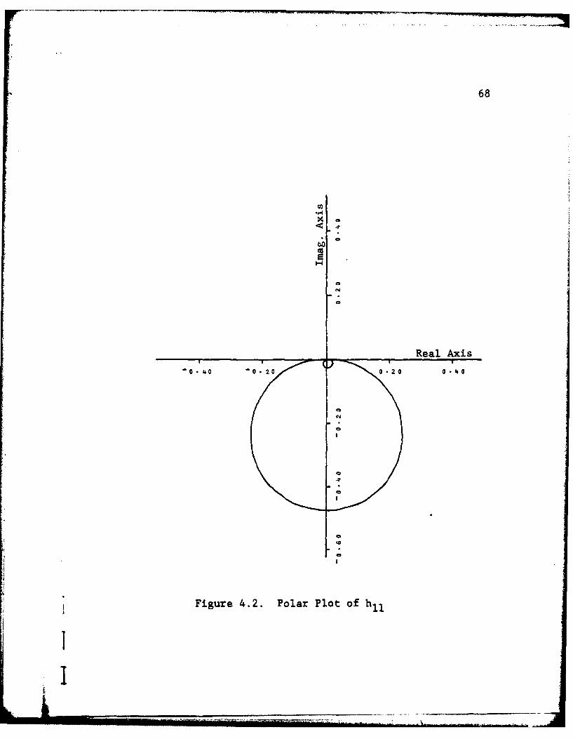
act with mode 1. Figure 4.2 is the polar plot for the

h1l frequency response of this problem. It appears at

first to be a plot of a single degree of freedom sys-

tem, however, a closer look reveals a very small re-

sponse circle near the origin. This domination can

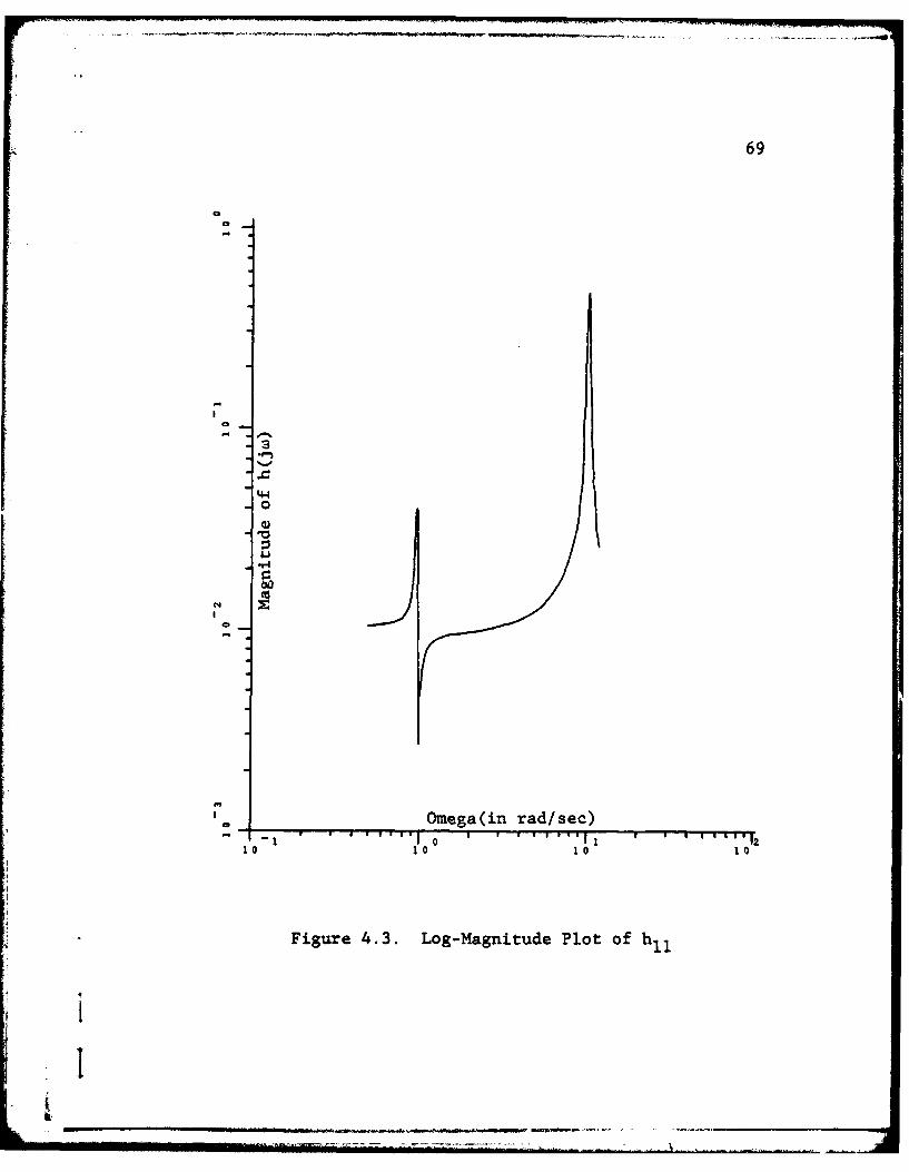
be seen more easily on the log-magnitude plot of Fig-

ure 4.3. This type of domination can be a problem if

the natural frequencies are close together.

The damping ratio in this problem was varied

from approximately 0.008 to approximately 0.20. The

exact solutions are tabulated in Appendix D.1 and the

curve fit estimations are given in Appendix D.2. As

68

C').

Figure 4.2. Polar Plot of l

69

4

0

0

.W-

4.,

o Omega(in rad/sec)

0 1 0 1 0 1O

Figure 4.3. Log-Magnitude Plot of hl

II

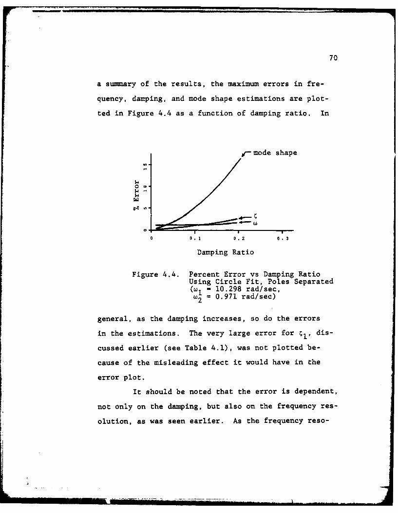
70

a summary of the results, the maximum errors in fre-

quency, damping, and mode shape estimations are plot-

ted in Figure 4.4 as a function of damping ratio. In

,-mode shape

$~400

4-

0 0.1 0.2 0.3

Damping Ratio

Figure 4.4. Percent Error vs Damping RatioUsing Circle Fit, Poles Separated(w = 10.298 rad/sec,

= 0.971 rad/sec)

general, as the damping increases, so do the errors

in the estimations. The very large error for 1' dis-

cussed earlier (see Table 4.1), was not plotted be-

cause of the misleading effect it would have in the

error plot.

It should be noted that the error is dependent,

not only on the damping, but also on the frequency res-

olution, as was seen earlier. As the frequency reso-

.. .. . . . .., , ,

71

lution is increased, the errors decrease. However, in

this study the frequency resolution was kept constant

and the error evaluated only as a function of damping.

The frequency resolution used for this problem was ap-

proximately 0.02 rad/sec.

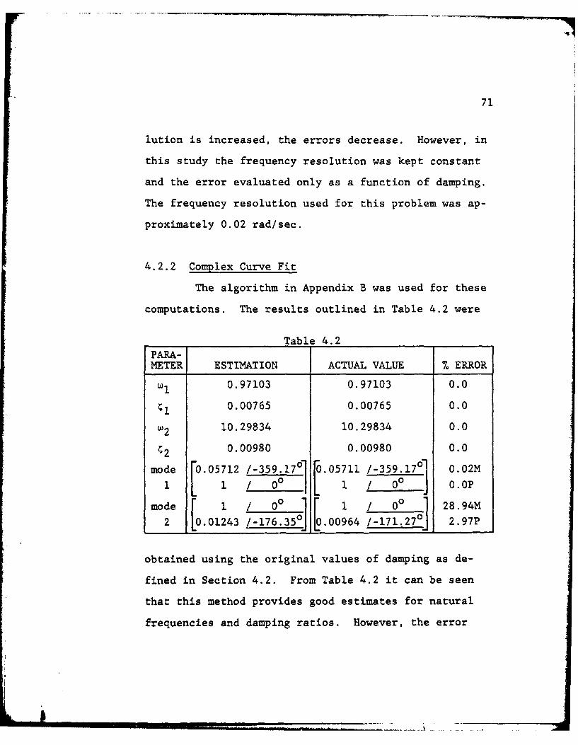
4.2.2 Complex Curve Fit

The algorithm in Appendix B was used for these

computations. The results outlined in Table 4.2 were

Table 4.2PARA-METER ESTIMATION ACTUAL VALUE % ERROR

W1 0.97103 0.97103 0.0

0.00765 0.00765 0.0

w2 10.29834 10.29834 0.0

2 0.00980 0.00980 0.0

mode [0.05712 /-359.17o1 .05711 /-359.17 O .02M

1 1 ____ 0__0_1_00 0.OP

mode [ 1 /0 0l / 00 28.94M2 .01243 /-176.35.j 0.00964 /-171.27O 2.97P

obtained using the original values of damping as de-

fined in Section 4.2. From Table 4.2 it can be seen

that this method provides good estimates for natural

frequencies and damping ratios. However, the error

72

in the 2nd mode shape gets larger as damping increases.

It is noted that the algorithm converged very slowly

on frequency response h21 . This points out one of the

problems with this technique. As noted earlier, one

mode dominates in this problem. When this situation

occurs, the initial estimates provided by the two

point estimation are not very accurate. As a result,

the convergence is either slow or non-existent. This

same problem can be encountered when the damping ratio

is increased.

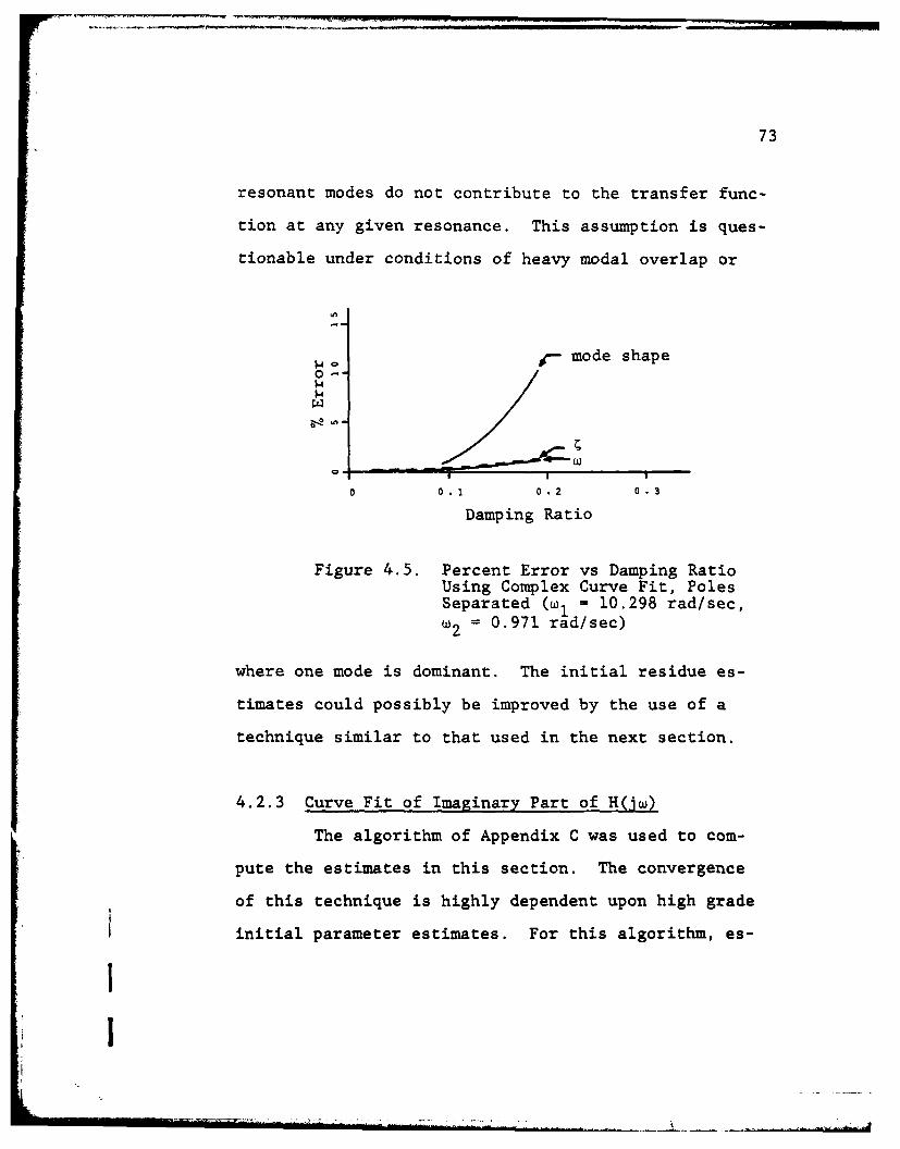
As in the previous section, the damping ratio

was varied from approximately 0.008 to 0.20 and the

results tabulated in Appendix D.3. Figure 4.5 is a

plot of the error vs damping for this algorithm. The

error in the mode shapes associated with the lack of

convergence were not plotted in order to avoid mis-

representation of the error vs damping. Again, as

the damping increased, the errors, in general, in-

creased for a fixed frequency resolution.

It appears that the main problem with this

method is that the initial estimates for the resi-

dues are sometimes not good enough to provide con-

vergence. The initial estimates for the residues are

calculated using the original assumption that off-

I!

, I'

73

resonant modes do not contribute to the transfer func-

tion at any given resonance. This assumption is ques-

tionable under conditions of heavy modal overlap or

4 C- mode shape0-

0. II

00.1 0.2 0.3

Damping Ratio

Figure 4.5. Percent Error vs Damping RatioUsing Complex Curve Fit, PolesSeparated (wi = 10.298 rad/sec,

= 0.971 rad/sec)

where one mode is dominant. The initial residue es-

timates could possibly be improved by the use of a

technique similar to that used in the next section.

4.2.3 Curve Fit of Imaginary Part of H(jw)

The algorithm of Appendix C was used to com-

pute the estimates in this section. The convergence

of this technique is highly dependent upon high grade

I initial parameter estimates. For this algorithm, es-

II

I •

0. . . . . . .0 1 . .. . . . . . . . .0 3'-

74

timates are required for the natural frequencies and

damping ratios only, since the algorithm computes the

initial estimates for the residues. If the initial

estimates of damping and natural frequency are more

than 10% in error, the algorithm may diverge using

this technique. For the purpose of this thesis, the

initial estimates were taken from the method of

Kennedy and Pancu (Circle Fit, Section 4.2.1). Except

for the case of inadequate frequency resolution, the

circle fit method gave good results for natural fre-

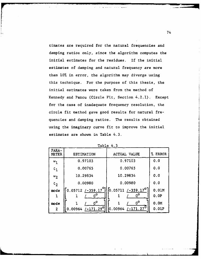
quencies and damping ratios. The results obtained

using the imaginary curve fit to improve the initial

estimates are shown in Table 4.3.

Table 4.3

PARA-METER ESTIMATION ACTUAL VALUE % ERROR

W1 0.97103 0.97103 0.0

I 0.00765 0.00765 0.0

w2 10.29834 10.29834 0.0

C2 0.00980 0.00980 0.0

mode [0.05712 /-359.17°1 [.05711 /-359.17 °" 0.01M111 / o0 J I . / 0° 0.0P

mode I / 0°0I / 00 0.0M

2 0.00964 /-171.29] 0.00964 /-171.27] 0.01P10

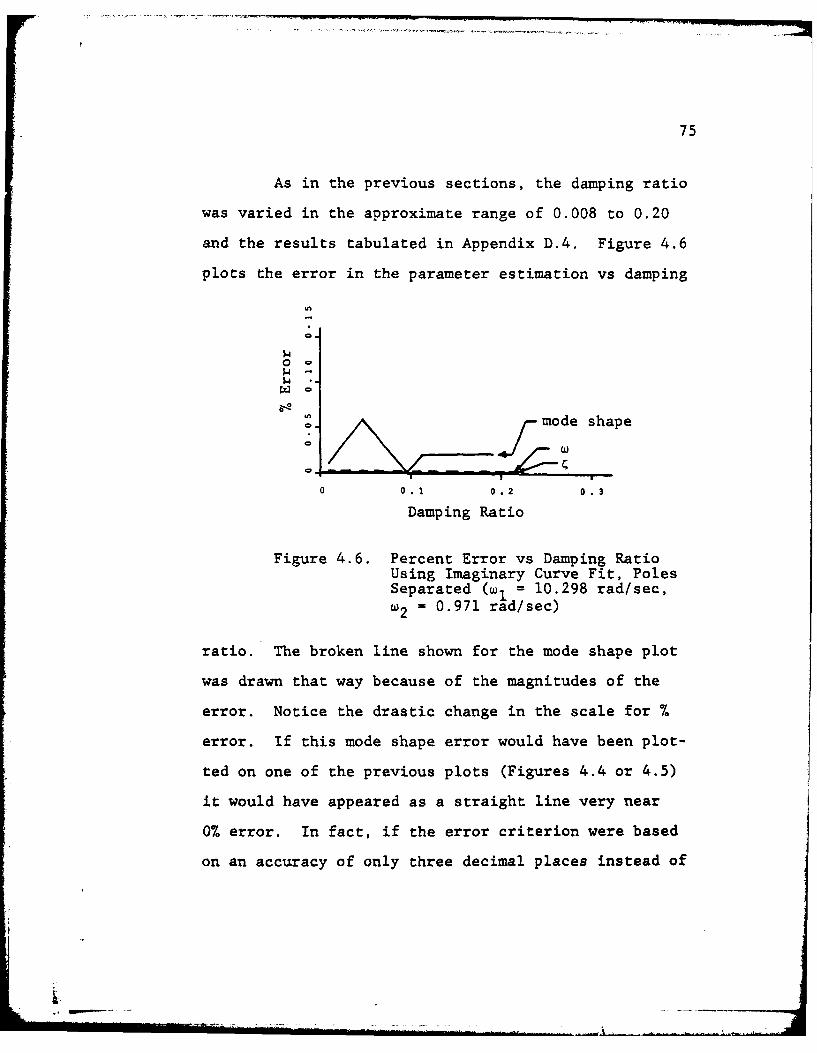
75

As in the previous sections, the damping ratio

was varied in the approximate range of 0.008 to 0.20

and the results tabulated in Appendix D.4. Figure 4.6

plots the error in the parameter estimation vs damping

a

0

mode shape

aW

00 1 0.2 0.3

Damping Ratio

Figure 4.6. Percent Error vs Damping RatioUsing Imaginary Curve Fit, PolesSeparated (wi = 10.298 rad/sec,w2 = 0.971 rad/sec)

ratio. The broken line shown for the mode shape plot

was drawn that way because of the magnitudes of the

error. Notice the drastic change in the scale for %

error. If this mode shape error would have been plot-

ted on one of the previous plots (Figures 4.4 or 4.5)

it would have appeared as a straight line very near

0% error. In fact, if the error criterion were based

on an accuracy of only three decimal places instead of

76

five (as used in this study) then there would be 0%

error for all parameter estimations in this problem.

The damping ratio was not increased any further

because of the difficulty in obtaining natural fre-

quencies and damping ratios. This is an area that

needs further research before the full limits of the

imaginary curve fit algorithm can be tested.

It can be seen that this method is more de-

sirable than the previous two methods, especially if

the mode shapes are of interest.

4.3 Example Problem Two

Using the same system as described in Figure

4.1, define the following variables:

m= 3 m2 = i

kI = 36 k2 ' 6

cI = .15 C2 = 0.05

For this system, the actual values for the modal pa-

rameters as computed via a complex eigen solver rou-

tine are:

i1 2.16993 rad/sec w2 3.91039 rad/sec

i _ _ _ __ __ _ _

77

I 0.00764 ;2 = 0.01068

mode 0.2526 /-359.4~10

0

0mode 2 =f I / 0

m.64593 /-178.940

The main difference between this problem and problem

one is spacing of the system poles. For this problem

the poles are close together compared to the separa-

tion in problem one.

As in the previous example problem, the fre-

quency response functions h1 1 and h2 1 were used to es-

timate the modal parameters. The frequency resolution

in this problem was approximately 0.01 rad/sec.

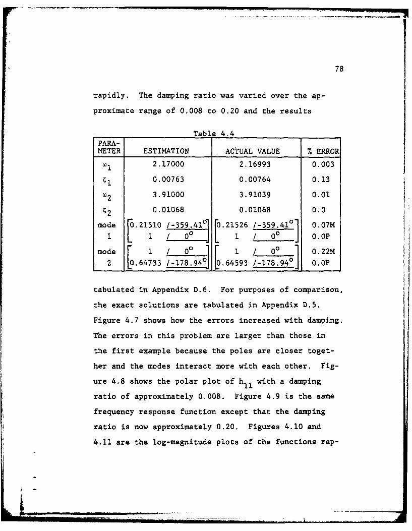
4.3.1 Method of Kennedy and Pancu (Circle Fit)

As in Section 4.2.1, the estimates for the

modal parameters were computed and the results pre-

sented in Table 4.4. One can immediately see that the

estimates are very good. The frequency resolution was

sufficient in this case to provide good estimates,

with the damping at a low level. However, as the

amount of damping increased, the accuracy dropped off

78

rapidly. The damping ratio was varied over the ap-

proximate range of 0.008 to 0.20 and the results

Table 4.4

PARA-METER ESTIMATION ACTUAL VALUE % ERROR

W1 2.17000 2.16993 0.003

0.00763 0.00764 0.13

w2 3.91000 3.91039 0.01

0.01068 0.01068 0.0

mode 250/394 21526 /-359.410 .7

1 L 1 0 J .0S 0o 0o

mode 0 11 0.22M2 .64733 /-178.940 .64593 /-178.94' 0,0P

tabulated in Appendix D.6. For purposes of comparison,

the exact solutions are tabulated in Appendix D.5.

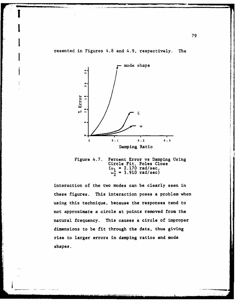
Figure 4.7 shows how the errors increased with damping.

The errors in this problem are larger than those in

the first example because the poles are closer toget-

her and the modes interact more with each other. Fig-

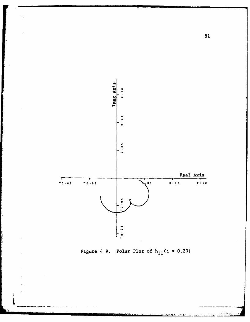
ure 4.8 shows the polar plot of h with a damping

ratio of approximately 0.008. Figure 4.9 is the same

frequency response function except that the damping

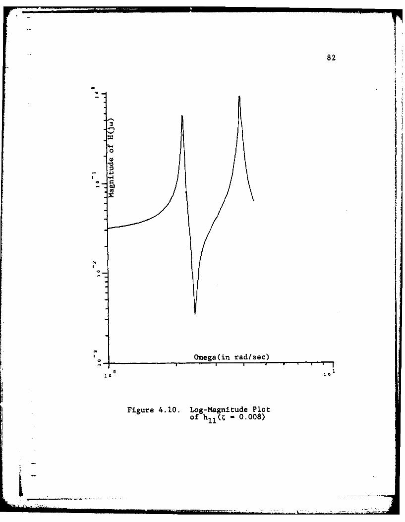
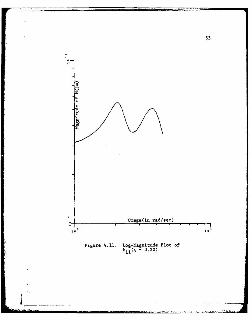
ratio is now approximately 0.20. Figures 4.10 and

4.11 are the log-magnitude plots of the functions rep-

79

resented in Figures 4.8 and 4.9, respectively. The

- mode shape

0 "

14r0-1.4

0.1 0.2 0.3

Damping Ratio

Figure 4.7. Percent Error vs Damping UsingCircle Fit, Poles Close(w, - 2.170 rad/sec,w2 - 3.910 rad/sec)

interaction of the two modes can be clearly seen in

these figures. This interaction poses a problem when

using this technique, because the responses tend to

not approximate a circle at points removed from the

natural frequency. This causes a circle of improper

dimensions to be fit through the data, thus giving

rise to larger errors in damping ratios and mode

shapes.

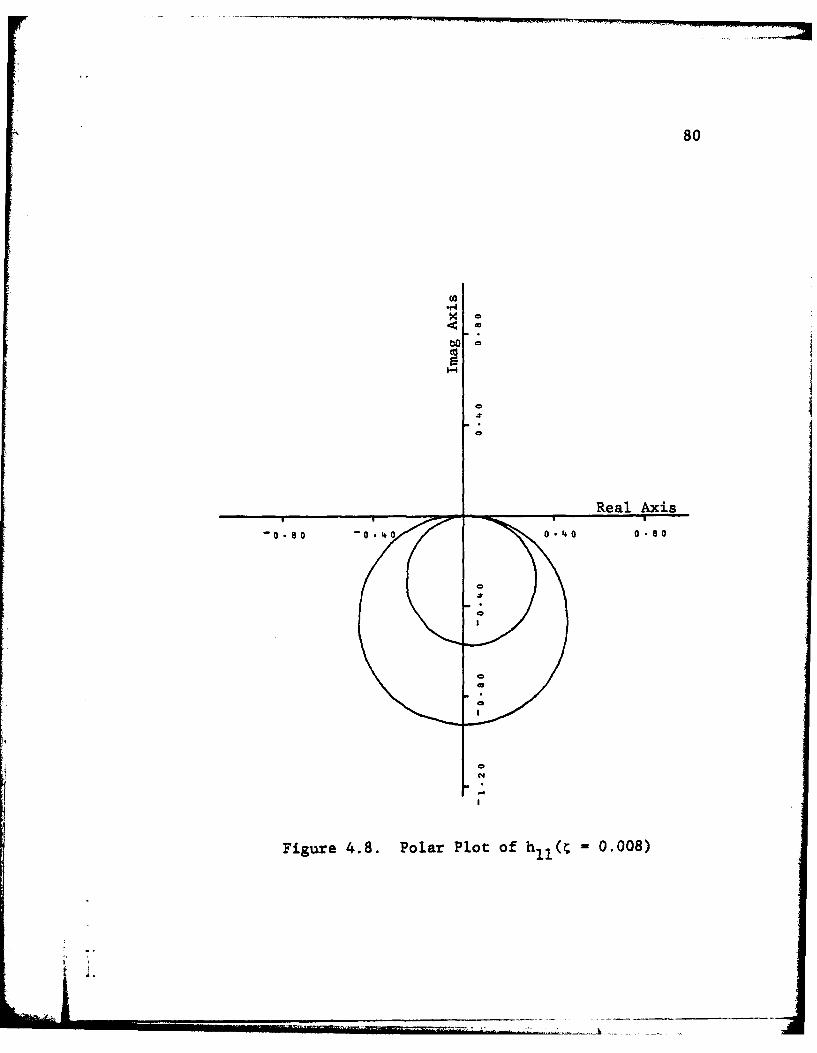
80

-,

1-4

Real Axis

-a80 0 -4 0 0.-4 0 0.8 a0

Figure 4.8. Polar Plot of h - 0.008)

81

-4

RelAi

0 - a - 1 1 - a 1

Figure .9. Poar lto i .0

82

4,

0

- 4.)",4

Omega(in rad/sec)

10 101

Figure 4.10. Log-Magnitude Plotof h 1 0.008)

83

0

100 1

Figure 4.11. Log-Magnitude Plot of-0.20)

84

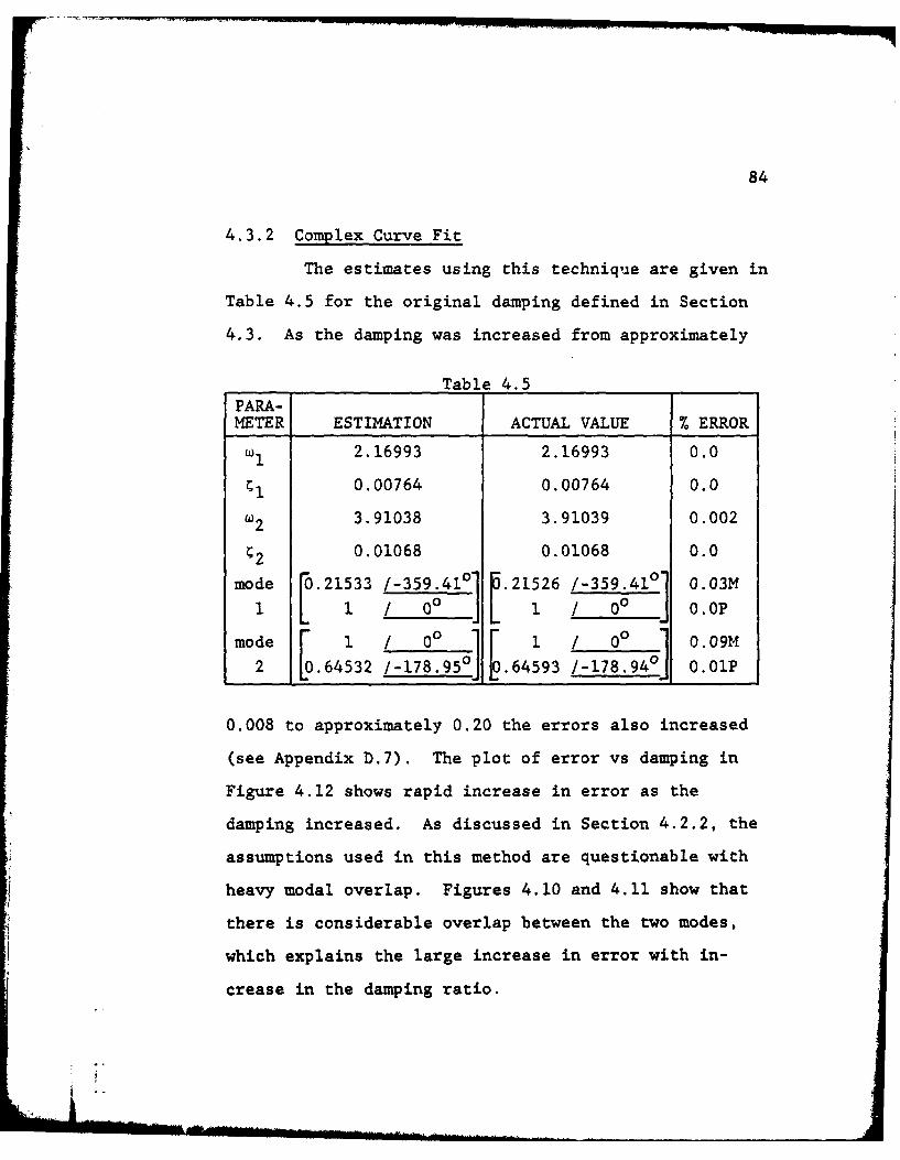
4.3.2 Complex Curve Fit

The estimates using this technique are given in

Table 4.5 for the original damping defined in Section

4.3. As the damping was increased from approximately

Table 4.5

PARA-METER ESTIMATION ACTUAL VALUE % ERROR

I 2.16993 2.16993 0.0

0.00764 0.00764 0.0

W2 3.91038 3.91039 0.002

2 0.01068 0.01068 0.0

mode U.21533 /-359.410 [.21526 /-359.4101 0.03M1 Ll /00] L / 0o 0 0.OP

mode r 1 / 00° 1 0 0 0.09M2m 0.64 532 /-178.95°] 0.64593 /-178.940] O.OP

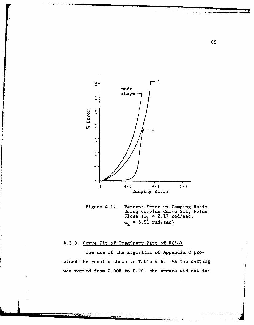
0.008 to approximately 0.20 the errors also increased

(see Appendix D.7). The plot of error vs damping in

Figure 4.12 shows rapid increase in error as the

damping increased. As discussed in Section 4.2.2, the

assumptions used in this method are questionable with

heavy modal overlap. Figures 4.10 and 4.11 show that

there is considerable overlap between the two modes,

which explains the large increase in error with in-

crease in the damping ratio.

85

modeshape --

0 '

0,4

0 0.1 0.2 0.3

Damping Ratio

Figure 4.12. Percent Error vs Damping RatioUsing Complex Curve Fit, PolesClose (wI = 2.17 rad/sec,

w2 f 3.91 rad/sec)

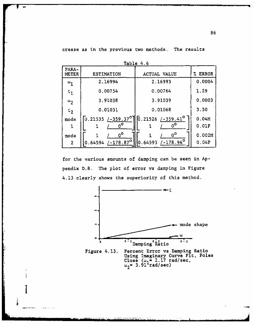
4.3.3 Curve Fit of Imaginary Part of H(Jw)

The use of the algorithm of Appendix C pro-

vided the results shown in Table 4.6. As the damping

was varied from 0.008 to 0.20, the errors did not in-

LL4

86

crease as in the previous two methods. The results

Table 4.6

PARA-METER ESTIMATION ACTUAL VALUE %~ ERROR

2.16994 2.16993 0.0004

0.00754 0.00764 1.29

W23.91038 3.91039 0.0003

20.01031 0.01068 3.50

mode [021535 /-359.37o1[0.21526 /-359.4101 0 .04M

1 Li 0o0 1 / 00 J 0.01Pmode / 0100 1 0.002M

2 0 [.64594 1~7 8.8][.64593 /-178.940J Q4

for the various amounts of damping can be seen in Ap-

pendix D.8. The plot of error vs damping in Figure

4.13 clearly shows the superiority of this method.

- - mode shape

0 O~lDminOi.tio 0:

Figure 4.13. Percent Error vs Damping RatioUsing Imaginary Curve Fit, PolesClose (w1- 2.17 rad/sec,

2-3 .91 rad/sec)

87

Caution must be exercised in using this meth-

od and choosing the initial estimates for natural fre-

quency and damping ratio. If the initial estimates are

greater than 10% in error, as mentioned earlier, there

is a possibility that the method will diverge.

4.4 Determination of Mass, Stiffness,and Damping Matrices

As an extension of example problem one, the

data from Section 4.2.3, with the damping ratio approx-

imately equal to 0.008, was used to determine the mass,

stiffness, and damping matrices. This example will

demonstrate the use of equations (2.21), (2.27), and

(2.31).

It has been shown that the modal properties

can be determined from frequency response data with

relatively good accuracy (depending on the method

used). The residue at each pole is measured and then

used to determine the mode shape. Recall from equa-

tion (2.10) that the residue matrix for mode k can

be written in terms of the normalized mode shape.

Ak a TSk-uk-u

Recall that the residue matrix can also be written as

AOA'91 459 AIR FORCE INST OF TECH WRIGHT-PATTERSON AFS OH F/G 12/1DETERMINATION OF MODAL PARAMETERS FROM EXPERIMENTAL FREQUENCY R--ETC(U)DEC 78 C V MILLER

UNCLASSIFIED AFIT-CF-79-182T NL

HIL

3L 136 2.2.6

11111L 5J=.I11 _ _.1,II1.

MICROCOPY RESOLUTION TEST CHARTNATIONAL BUREAU OF STANDARDS- 1963-A

88

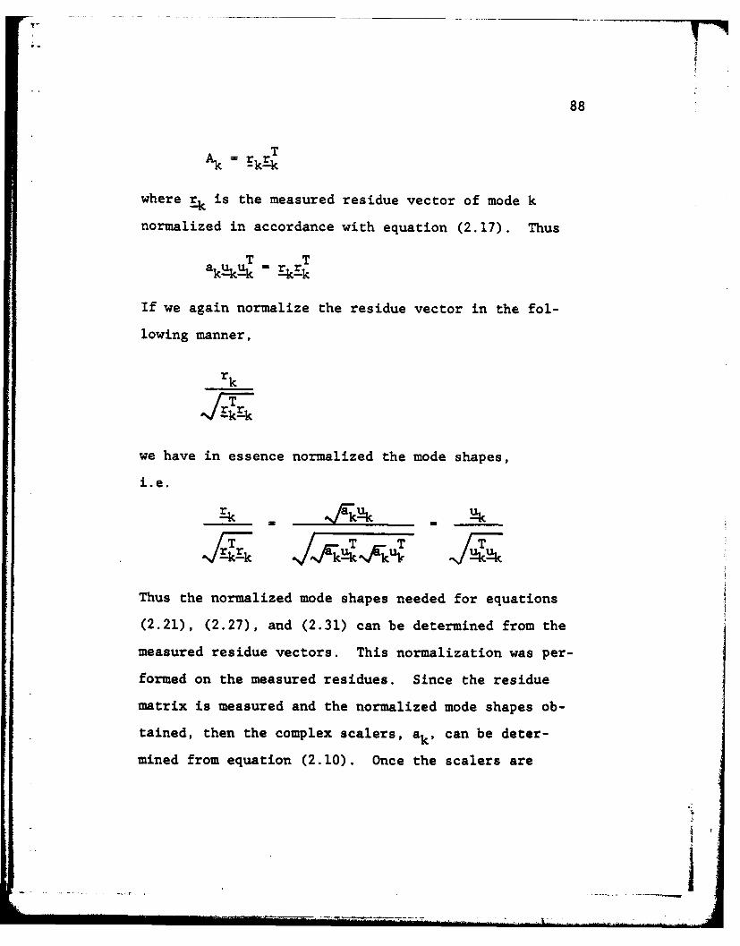
Ak Sk~k

where sk is the measured residue vector of mode k

normalized in accordance with equation (2.17). Thus

T Takik-u' Ek~k

If we again normalize the residue vector in the fol-

lowing manner,

rk

we have in essence normalized the mode shapes,

i.e.

Thus the normalized mode shapes needed for equations

(2.21), (2.27), and (2.31) can be determined from the

measured residue vectors. This normalization was per-

formed on the measured residues. Since the residue

matrix is measured and the normalized mode shapes ob-

tained, then the complex scalers, ak, can be deter-

mined from equation (2.10). Once the scalers are

~ij

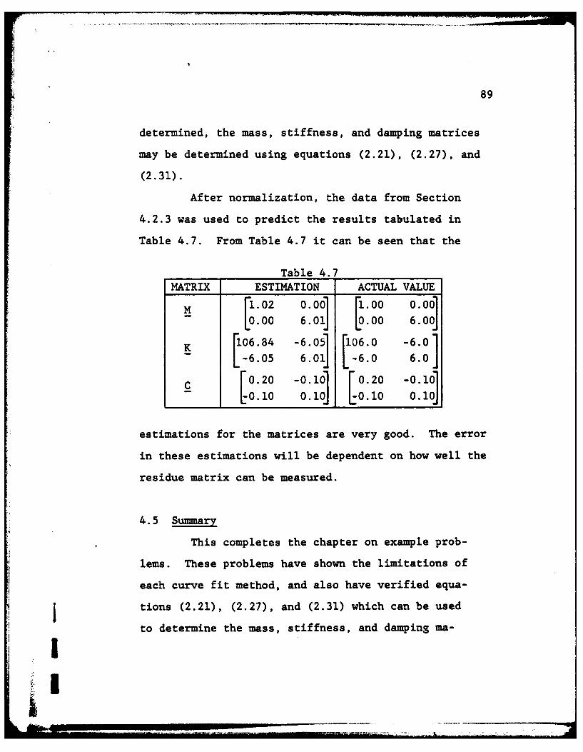
89

determined, the mass, stiffness, and damping matrices

may be determined using equations (2.21), (2.27), and

(2.31).

After normalization, the data from Section

4.2.3 was used to predict the results tabulated in

Table 4.7. From Table 4.7 it can be seen that the

Table 4.7

MATRIX ESTIMATION ACTUAL VALUE

M .02 0.00 .00 0.00J-0 .00 6.0 1 0 .00 6.00

K 106.84 -6.05] 06.0 -6.0-- 6.05 6.0 1 -6.0 6.0

0.20 -0.10 0.20 -0.10

- [0.20 0.10 0.10 0.10

estimations for the matrices are very good. The error

in these estimations will be dependent on how well the

residue matrix can be measured.

4.5 Sunnary

This completes the chapter on example prob-

lems. These problems have shown the limitations of

each curve fit method, and also have verified equa-

j tions (2.21), (2.27), and (2.31) which can be used

to determine the mass, stiffness, and damping ma-

i _

90

trices. The next chapter will review the results pre-

sented and draw conclusions on which curve fit method

is best under given conditions.

LI

i I I

CHAPTER V

SUMMARY AND CONCLUSIONS

Four techniques were described in Chapter III

for estimating the natural frequencies, damping ratios,

and mode shapes of a system using the frequency re-

sponse functions measured at various points in the sys-

tem. The first method discussed dealt only with the

quadrature response and is only useful in very special

cases. The other three techniques were investigated

in more detail. The three curve fitting methods were

used to solve two example problems, one with the sys-

tem poles separated in frequency by approximately 10

rad/sec, and the other with the poles separated in

frequency by approximately 1.7 rad/sec. These exam-

ple problems pointed out the usefulness of the differ-

ent techniques.

The method of Kennedy and Pancu (circle fit)

provided very good estimates for natural frequencies

and damping ratios, provided that the frequency reso-

lution is adequate. However, if the mode shapes are

also desired, this method begins to break down. It

91

L

92

was shown in Sections 4.2.1 and 4.3.1 that, when there

is heavy modal overlap or when one mode dominates, the

method yields large errors. For example, with the

poles separated in frequency by approximately 10 rad/

sec, a frequency resolution of approximately 0.02 rad/

sec, and with a damping ratio of approximately 0.008,

the error in the damping ratio estimate was 368%.

This was due to inadequate frequency resolution in a

problem where one mode dominated. When the poles were

separated by approximately 1.7 rad/sec in frequency

and with the damping ratio near .20, and a frequency

resolution of approximately 0.01 rad/sec, this method

produced an error of 168% in the mode shape of mode 2.

However, under the same conditions, the natural fre-

quency estimations were in error by less than 3% and

the damping ratios were in error by less than 87.

It is concluded that the method of Kennedy and

Pancu is reliable for estimating the natural frequen-

cies and damping ratios except in the cases where one

mode dominates or when the damping ratio exceeds 0.20.

The complex curve fit method also provided

.resonable estimates under certain conditions. For

I instance, when the poles were separated in frequency

by 10 rad/sec, with 8% damping and 0.02 rad/sec fre-

!

&

93

quency resolution, the errors for natural frequencies,

damping ratios, and mode shapes were all less than 1%.

However, with the damping at 3.8%, and the other fac-

tors as above, this method produced an error of 198

in the estimation of mode shape 2 while maintaining

less than 1% error in other parameters. This large

error was due to a lack of convergence (in 50 itera-

tions) of the technique used. This method makes use

of an assumption that is not valid when one mode dom-

inates or when the degree of modal overlap is heavy.

It is this assumption that causes the large errors to

be generated. For example, with the poles separated

in frequency by 1.7 rad/sec, damping set at 0.20, and

a frequency resolution of 0.01 rad/sec, this method

yielded errors in mode shapes as large as 747. and

errors in natural frequencies and damping ratios as

high as 16 and 88%, respectively.

It is concluded that the complex curve fit

works well under the conditions of light modal over-

lap provided that no one mode dominates the response.1When one mode dominates, the estimates are still good

for the natural frequencies and damping ratios, but

the estimates for the mode shapes are not reliable.

When the poles are close together where they interactI£ __ __ _ __ __ _

1..94

to form the total response, this technique is not very

reliable. The errors, again, are due primarily to

poor initial estimates (computed based on an assump-

tion that is invalid for heavy modal overlap) for

which the algorithm converges to the wrong values.

A modified complex curve fit method could be

investigated by using a method similar to that dis-

cussed in Section 4.2.3 to provide the initial esti-

mates for the previously described complex curve fit.

This could possibly make this method more desireable.

The final method discussed, that of curve fit-

ting the imaginary part of the frequency response,

provided excellent results for all cases considered.

The maximum error for any parameter or mode shape was

less than 4% for all cases considered. These cases

included the poles separated in frequency by 10 rad/

sec, a frequency resolution of 0.02 rad/sec, and the

damping ratio varying from 0.008 to 0.20. They also

included the cases where the poles were separated in

frequency by 1.7 rad/sec and the frequency resolution

was 0.01 rad/sec, with the damping ratio varying from

0.008 to 0.20. The results obtained using this tech-

nique makes this method the most desireable of the

three methods discussed. The main problem associated

--1'

95

with this method is that it diverges if the initial es-

timates for natural frequencies and damping ratios are

in error by more than 10%. Therefore caution must be

used when determining the initial estimates required

to start this method. It has been found that, in all

cases considered, if the method converged, it did so

with excellent results. Therefore, a trial and error

type approach could be taken, if necessary, to deter-

mine the initial estimates. If the method diverges,

then another estimate could be tried until convergence

is obtained.

In suumary, if only the natural frequencies

and damping ratios are desired, the method of Kennedy

and Pancu provides acceptable results, except where

one mode is dominant. However, if the mode shapes are

also desired, then the curve fit of the imaginary re-

sponse is the most desireable from the standpoint of

minimum error.

iv.

_ _ _ _ _ 1 z - -

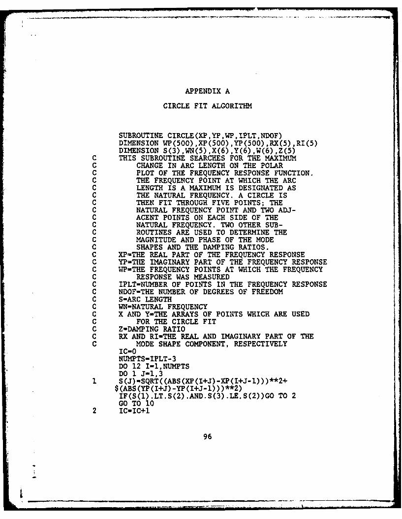
APPENDIX A

CIRCLE FIT ALGORITHM

SUBROUTINE CIRCLE (XP, YP ,WP, IPLT, NDOF)DIMENSION WP(500),XP(500),YP(500),RX(5),RI(5)DIMENSION S(3),WN(5),X(6),Y(6),W(6),Z(5)

C THIS SUBROUTINE SEARCHES FOR THE MAXIMUMC CHANGE IN ARC LENGTH ON THE POLARC PLOT OF THE FREQUENCY RESPONSE FUNCTION.C THE FREQUENCY POINT AT WHICH THE ARCC LENGTH IS A MAXIMUM IS DESIGNATED ASC THE NATURAL FREQUENCY. A CIRCLE ISC THEN FIT THROUGH FIVE POINTS; THEC NATURAL FREQUENCY POINT AND TWO ADJ-C ACENT POINTS ON EACH SIDE OF T1HEC NATURAL FREQUENCY. TWO OTHER SUB-C ROUTINES ARE USED TO DETERMINE THEC MAGNITUDE AND PHASE OF THE MODEC SHAPES AND THE DAMPING RATIOS.C XP-THE REAL PART OF THE FREQUENCY RESPONSEC YP-THlE IMAGINARY PART OF THE FREQUENCY RESPONSEC WP-THE FREQUENCY POINTS AT WHICH THE FREQUENCYC RESPONSE WAS MEASUREDC IPLT-NUMBER OF POINTS IN THE FREQUENCY RESPONSEC NDOF=THE NUMBER OF DEGREES OF FREEDOMC S-ARC LENGTHC WN=NATURAL FREQUENCYC X AND Y-THE ARRAYS OF POINTS WHICH ARE USEDC FOR THE CIRCLE FITC Z-DAMPING RATIOC RX AND RI-THE REAL AND IMAGINARY PART OF THEC MODE SHAPE COMPONENT, RESPECTIVELY

IC-ONUMPTS-IPLT- 3DO 12 I-1,NUMPTSDO 1 J-1,3

1 S(J)-SQRT((ABS(XP(I+J)-XP(I+J-1)))**2+$(ABS(YP(I+J)-YP(I+J-1)))**2)IF(S(1).LT.S(2).AND.S(3).LE.S(2))GO TO 2GO TO 10

2 IC-IC+l

96

7 IL. .. . ._ i

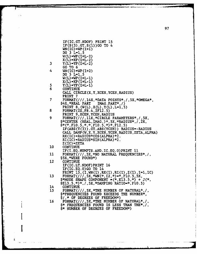
97

IF(IC.GT.NDOF) PRINT 15IF(S(3).GT.S(1))GO TO 4WN (IC) -WP (I+l)DO 3 L-1,5W(L)-WP (I+L-2)X (L)-=XP (I+L- 2)

3 Y (L) -YP (I+L- 2)GO TO 6

4 WN (IC) =WP (I+2)DO 5 L-1,5W(L)-WP(I+L-1)X(L)-XP (I-9L-1)

5 Y(L)-YP(I+L-1)6 CONTINUE

CALL CIRCLE (X, Y, XCEN, YCEN, RADIUS)PRINT 7

7 FORMAT(///,14X,*DATA POINTS*,/,5X,*OMEGA*,$4X,*REAL PART IMAG.PART*,/)PRINT 8, (W(L) ,X(L) ,Y(L) ,L-1,5)

8 FORMAT(2X,F8.4,2Fl2.5)PRINT 9, XCEN, YCEN, RADIUS

9 FORMIAT(///,11X,*CIRCLE PARAMETERS*,/,5X,$*CE-NTER (REAL,IMAG.)*,5X,*RADIUS*,/,2X,$*(*,F1O.5,*,*.F1O.5,*)*,F12.5)IF(ABS(Y(3)) .GT.ABS(YCEN)) RADIUS--RADIUSCALL DAMP(W,X,Y,XCCEN,YCEN,RADIUS,ZETA,ALPHA)RX(IC)=RADIUS*COS (ALPHA) *2.RI (IC) =RADIUS*SIN (ALPHA) *2.Z (IC) -ZETA

1.0 CONTINUEIF(I.EQ.NUMPTS.AND.IC.EQ.O)PRINT 11.

11 FORMAT(//I,5X,*NO NATURAL FREQUENCIES*,/,$5X,*ERE FOUND*)

12 CONTINUEIF(IC.LT.NDOF)PRINT 16IF(IC.EQ.0)GO TO 14IPRINT 13,(I,WN(I),RX(I),RI(I),Z(I),I-1,IC)

13 FORMT(///,5X,*WN(*,I2,*)=*,Fl0.5,5X,$*MODE SHAPE COMPONENT -(*,E13.5,*) + J(*,$E13.5,*)*,/,5X,*DAMPING RATIO-*,FlO.5)

14 CONTINUE15 FOMAT(///,5X,*THE NUMBER OF NATURAL*,/,

$*FREQUENCIES FOUND EXCEEDS THE NUMBER*,$/,* OF DEGREES OF FREEDOM*)

16 FOPMAT(///,5X,*TUE NUMBER OF NATURAL*,/,$* FREQUENCIES FOUND IS LESS THAN THE*,/,$* NUMBER OF DEGREES OF FREEDOM*)

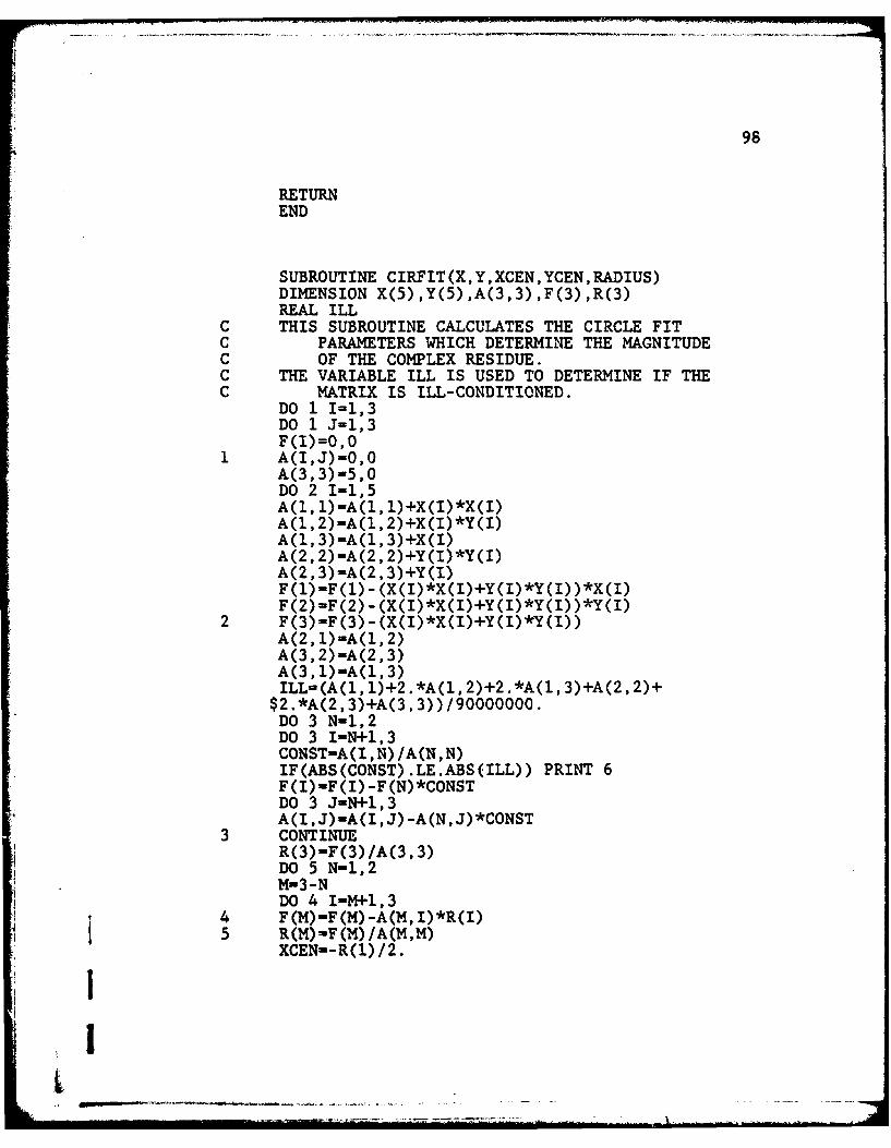
98

RETURNEND

SUBROUTINE CIRFIT (X, Y, XCEN ,YCEN ,RADIUS)DIMENSION X(5),Y(5),A(3,3),F(3),R(3)REAL ILL

C THIS SUBROUTINE CALCULATES THE CIRCLE FITC PARAMETERS WHICH DETERMINE THE MAGNITUDEC OF THE COMPLEX RESIDUE.C THE VARIABLE ILL IS USED TO DETERMINE IF THEC MATRIX IS ILL-CONDITIONED.

DO 1 I=1,3DO 1 J-1,3F(I)=O,O

1 A(I,J)=O,OA(3,3)=5,0DO 2 1-1,5A(i, 1)=A(i, 1)+X(I)*X(I)A(1, 2)-A(1,2)+X(I)*Y(I)A (1, 3) =A(1, 3) +X(I)A(2, 2)-A(2, 2)+Y(I)*Y(I)A(2, 3)=A(2, 3)+Y(l)F(1)-F(l) -(X(I)*X(I)+Y(I)*Y(I) )*X(I)F(2)-F(2) -(X(I)*X(I)+Y(I)*Y(I) )*Y(I)

2 F(3)-F(3)-(X(I)*X(I)+Y(I)*Y(I))A(2, 1)=A(1, 2)A (3, 2)-A (2, 3)A (3, 1) =A (1, 3)ILL-(A(1, 1)+2 *A(1,2)+2.*A(1,3)+A(2 ,2)+

$2.*A(2, 3)+A(3 ,3)) /90000000.DO 3 N-1,2DO 3 I-N+1,3CONST-A(I ,N) /A(N,N)IF(ABS(CONST).LE.ABS(ILL)) PRINT 6F(I)-F(I) -F(N)*CONSTDO 3 J-N+1,3A(I,J)-A(I,J) -A(N,J)*CONST

3 CONTINUER(3)-F(3)/A(3, 3)DO 5 N-1,2M-3- NDO 4 I-M+1,3

4 F(M)-F(M)-A(M,I)*R(I)5 R(M)-F(M)/A(M,M)

XCEN--R(1)/2.

99

YCEN--R(2) /2.RADIUS-SQRT (XCEN*XCEN+YCEN*YCEN-R(3))

6 FORMAT(1H1,5X,*THE COEFFICIENT MATRIX IS*,/,$5X,*ILL-CONDITIONED OR SINGULAR*, /,5X,$*AND THE SOLUTION MAY BE MEANINGLESS*)RETURNEND

SUBROUTINE DAMP(W,X,Y,XC,YC,R,Z,A)DIMENSION W(5) ,X(5) ,Y(5)

C THIS SUBROUTINE DETERMINES THE DAMPING RATIOC AND THE PHASE ANGLE OF THE COMPLEX RESIDUE.C XC=X-COORDINATE OF THE CIRCLE CENTERC YC=Y-COORDINATE OF THE CIRCLE CENTERC R=RADIUS OF THE CIRCLEC Z=DAMPING RATIOC A=PHASE ANGLE IN RADIANS

ClSQ=(X(3) -X(2) )*(X(3) -X(2) )+(Y(3) -$Y(2) )*(Y(3) -Y(2))C2SQ=(X(4) -X(3) )*(X(4) -X(3) )+(Y(4) -$Y(3) )*(Y(4)-Y(3))Sl=(SQRT(CISQ)) /2.S2=(SQRT(C2SQ)) /2.B1=SQRT (R**2-S 1**2)B2=SQRT (R**2-S2**2)THETA1=2.*ATAN2(S1,Bl)THETA2-2 .*A'TfA2(S2 ,B2)PHI1=(3. 14159265-THETAl) /2.PH12-(3 .14159265+"lHETA2) /2.BETA1=W(2) /W(3)BETA2=W(4) /W(3)

$ (2. *BETA1)Z2-((1. -BETA2**2)*SIN(PHI2)/COS(PHI2))/

$ (2. *BETA2)Z=(Z1+Z2) /2.XX2-ABS(X(3) -XC)YY2-ABS(Y(3) -YC)IF(Y(3).GT.YC)GO TO 1A-ATAN2 (XX2 ,YY2)IF(X(3) .LT.XC)A--AGO TO 2

1 A-ATAN2(YY2,XX2)+1.57079632IF(X(3) .LT.XC)A--A

2 CONTINUE

100

RETURNEND

APPENDIX B

MULTI DEGREE OF FREEDOM CURVE FIT ALGORITHM

SUBROUTINE HJW (XP, YP, WP, IPLT, NDOF)DIMENSION WP(500),XP(500),YP(500)DIMENSION W1(5),W2(5),HIR(5) ,HlI(5)DIMENSION H2R(5),H21(5),W-7N(5),RR(5),RI(5)DIMENSION SR(5,2),SI(5),AR(5),AI(5),Z(5)

C THIS SUBROUTINE PICKS OUT THE PEAKS INC THE IMAGINARY PART OF THE FREQUENCYC RESPONSE. TWO POINTS, ONE ON EACHC SIDE OF THE PEAK, ARE PICKED FORC EACH PEAK. THESE POINTS ARE THENC USED IN THE TWO POINT ESTIMATIONC TECHNIQUE.C XP-REAL PART OF THE FREQUENCY RESPONSEC YP=IMAGINARY PART OF THE FREQUENCYC RESPONSEC WP=FREQUENCY POINTS AT WHICH THE FRE-C QUENCY RESPONSE WAS MEASUREDC IPLT=NUMBER OF POINTS IN THE FREQUENCYC RESPONSEC NDOF=NUMBER OF DEGREES OF FREEDOM

NUMPTS=IPT- 2NPEAKS=ODO 6 I-1,NUMPTSIF(NPEAKS.GT.NDOF) PRINT 29IF(ABS(YP(I+1)).GE.ABS(YP(I)).AND.ABS(YP(I+$2)).LE.ABS(YP(I+I))) GO TO 1GO TO 4

1 NPEAKS=NPEAKS+1DO 2 JJ-1,2IJK=I+1-JJIJK-I+1+JJRATIOl-ABS (YP (I+1)/YP (IJK))IF(RATIO1.GE.1.0592537)GO TO 3

2 CONTINUE3 Wi (NPEAKS) =WP (IJK)

W2 (NPEAKS)-WP (IJL)H1R(NPEAKS)=XP(IJK)HII (NPEAKS) -YP (IJK)

1101II

102

H2R(NPEAKS) -XP (IJL)H21 (NPEAKS)-=YP (IJL)

4 CONTINUEIF(NPEAXS.EQ.O.AND.I.EQ.NUMPTS)PRINT 5

5 FORbAT(//,5X,*NO NATURAL FREQUENCIES*,/,5X,$*WERE FOUND*)

6 CONTINUEIF(NPEAKS.EQ.0)GO TO 28PRINT 7,NPEAKS

7 FORMAT(1Hl, 5X, 12,* RESONANT FREQUENCIES*, /,$5X,*WERE FOUND*)PRINT 8

8 FORMAT(//,5X,*POINTS USED IN ESTIMATION*,$/,7X,*(2 PER PEAK)*)DO 9 IJ=1,NPEAKS

9 PRINT 10,IJ,H1R(IJ) ,HII(IJ) ,IJ,H2R(IJ) ,H2I(IJ)10 FORMAT(/,5X,*H1(*,I2,*)= (*,El3.5,*)+

$J(*,El3.5,*)*,/,5X,*H2(*,I2,*)- *$El3.5,*)+J(*,El3.5,*)*)DO 11 IJ=1,NPEAKSSR(IJ,1)-0.ORR(IJ)=O. 0

11 RI(IJ)=O.ONN= 1

12 CONTINUEDO 13 MP-1,NPEAKST=H1R (NP) -RR(MP)D-H1I(MP) -RI (NP)E-H2R(MP) -RR(MP)F-H21(MP)-RI(MP)G=H1R(MP) -H2R (NP)P-HlI (NP) -H21 (NP)SR(NPT,2)-((W2(MP)*F-W1(MP)*D)*G,+(Wl(NP)*T-$W2(MP)*E)*P) /(G*G+P*P)SI(NP)-((Wl(NP)*T-W2(MP)*E)*G- (W2(NP)*F-$W1 (NP) *D) *P) /(G*G+P*P)AR(MP)=0.5*(-(SR(MP,2)*(T+E)+D*(Wl(MP)-$sI(MP) )+F* (W2 (NP) -SI(NP))))AI(NP)=O. 5*(T*(W1(NP)-.SI(NP))+E*(W2(NP)-$SI (NP)) -SR(NP, 2)*(D+F))

13 CONTINUEICON-0DO 14 JCT-1,NPEAKSDIFF-ABS (SR(JCT, 2) -SR(JCT, 1))IF (DIFF.LE. .000001) ICON-ICON+1IF(ICON.EQ.NPEAKS)GO TO 25

14 CONTINUE

103

RPR-O. 0RPI-O. 0IF(NN.EQ.l)GO TO 17DO 16 I-1,IPLTSUMR-O.OSUIMI=O.ODO 15 J-1,NPEAKsZ1--2 .*(AR(J)*SR(J, 2)+AI(J)*SI(J))Z2-2 . *WP(I)*AR(J)Z3-SR(J, 2)*SR(J, 2)+SI (J)*SI (J)-WP (I)*WP (I)Z4-2.*WP(I)*SR(J, 2)SMR-SUMR+( (Zl*Z3-Z2*Z4)/I(Z3*Z3+Z4*Z4))SUMI-SUMI+( (Z2*Z3+Z1*z4) /(Z3*Z3+Z4*Z4))

15 CONTINUERPR-RPR+XP (I) -SUMRRPI-RPI+YP (I) -SUMI

16 CONTINUERIPLT= FLOAT (IPLT)RPR=RPR/ RIPLTRPI=RPI/RIPLT

17 CONTINUEDO 21 IM=1,NPEAKSRBR=O.0RBI-O.ODO 20 NR=1,,2W-1-W1 (M.R)IF(NR. EQ. 2) WW=W2(MR.)RBCR-C- (AR(MR) *SR(MR, 2)) -Al (MR.)*(WW%+

$SI(MR)))/ (SR(MR,2)*SR(MR,2)+(WW+

RBCI= (Al (MR)*SR(MR, 2)-AR(IIR)*(WW+$SI (MR.))) /(SR(MR, 2)*SR(MR, 2)+(WW+

SUMR-O.0

IF(PES.EQ.1)TO TO 19DO 18 KR-1,NPEAKSIF(KR.EQ.MR)GO TO 18Q1=-2 .*(AR(KR)*SR(KR, 2)+AI (KR)*SI (KR))Q2-2 *WW*AR(KR)Q3-SR(KR, 2)*SR(KR, 2)+SI(KR)*SI(KR) -WW*WWQ4-2.*WW*SR(yJR 2)DENOM-Q3*Q3+Q4*Q4SUMR-SUMR+( (Q1*Q3-Q2*Q4) /DENOM)SUMI-SUMI+( (Q2*Q3+Q1*Q4) /DENOM)

18 CONTINUE19 RBR-RBR+RBCR+SUMR

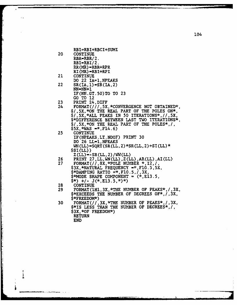
104

RBI=RBI+RBCI+SUMI20 CONTINUE

RBR=RBR/ 2.RBI-RBI/2.RR(MR) -RBR+RPRRI (MR) -RBI+RPI

21 CONTINUEDO 22 IA=1,NPEAKS

22 SR(IA,1)-SR(IA,2)NN=NN+IIF(NN.GT.50)TO TO 23GO TO 12

23 PRINT 24,DIFF24 FORMAT(///,5X,*CONVERGENCE NOT OBTAINED*,

$/,5X,*ON THE REAL PART OF THE POLES ON*,$/,5X,*ALL PEAKS IN 50 ITERATIONS*,//,5X,$*DIFFERENCE BETWEEN LAST TWO ITERATIONS*,$/,5X,*ON THE REAL PART OF THE POLES*,/,$5X,*WAS =*,Fl4.6)

25 CONTINUEIF(NPEAKS.LT.NDOF) PRINT 30DO 26 LL=1,NPEAKSWN(LL)-SQRT(SR(LL, 2)*SR(LL, 2)+SI(LL)*$SI(LL))Z(LL)=-SR(LL, 2)/WW(LL)

26 PRINT 27,LL,WN(LL) ,Z(LL) ,AR(LL) ,AI(LL)27 FORMAT(//,8X,*POLE NUMBER *,12,/,

$3X,*NATURAL FREQUENCY =*,FIO.5,5X,$*DAMPING RATIO =*,F1O.5,/,3X,$*MODE SHAPE COMPONENT = (*,E13.5,$*) +/- J(*,E13.5,*)*)

28 CONTINUE29 FORMAT(lH1,3X,*THE NUMBER OF PEAKS*,/,3X,

$*EXCEEDS THE NUMBER OF DEGREES OF*,/,3X,$*FREEDOM*)

30 FORMAT(//,3X,*THE NUMBER OF PEAKS*,/,3X,$*IS LESS THAN THE NUMBER OF DEGREES*,/,$3X,*OF FREEDOM*)RETURNEND

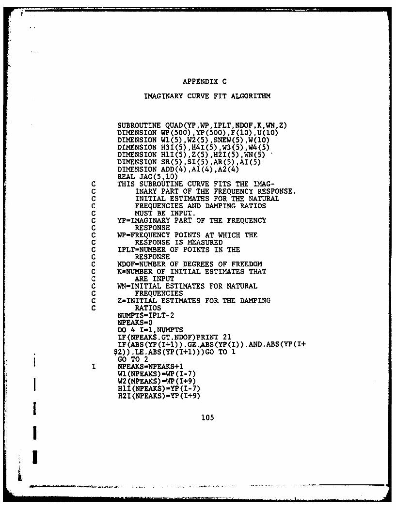
APPENDIX C

IMAGINARY CURVE FIT ALGORITHM

SUBROUTINE QUAD(YP,WP,IPLT,NDOF,K,WN,Z)DIMENSION WP(500),YP(500),F(10),U(10)DIMENSION Wi(5),W2(5),SNEW(5) ,W(10)DIMENSION H31(5),H4I(5),W3(5),W4(5)DIMENSION HII(5) ,Z(5) ,H2I(5) ,WN(5)DIMENSION SR(5),SI(5),AR(5),AI(5)DIMENSION ADD(4),A1 (4),A2(4)REAL JAC(5,1 0)

C THIS SUBROUTINE CURVE FITS THE IMAG-C INARY PART OF THE FREQUENCY RESPONSE.C INITIAL ESTIMATES FOR THE NATURALC FREQUENCIES AND DAMPING RATIOSC MUST BE INPUT.C YP-IMAGINARY PART OF THE FREQUENCYC RESPONSEC WP-FREQUENCY POINTS AT WHICH THEC RESPONSE IS MEASUREDC IPLT-NUMBER OF POINTS IN THEC RESPONSEC NDOF-NUMBER OF DEGREES OF FREEDOMC K-NUMBER OF INITIAL ESTIMATES THATC ARE INPUTC WN-INITIAL ESTIMATES FOR NATURALC FREQUENCIESC Z-INITIAL ESTIMATES FOR THE DAMPINGC RATIOS

NUMPTS-IPLT- 2NPEAKS-0DO 4 I-1,NUMPTSIF(NPEAKS. GT.NDOF)PRINT 21IF(ABS(YP(I+1)).GE.,ABS(YP(I)) .AND.ABS(YP(I+

$2)).LE.ABS(YP(I+1)))GO TO 1GO TO 2

1 NPEAKS-NPEAKS+1Wl (NPEAKS)-WP (I-7)W2 (NPEAKS) -WP (1+9)lI (NPEAKS)-Y (I-7)

121 (NPEAKS) -Yp (I+9)

105

ij

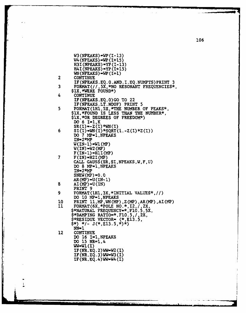
106

W3(NPEAKS)-WP(I-13)W4(NPEAKS)-WP (1+15)H31 (NPEAKS)-YP (I-13)1141(NPEAKS)-YP (1+15)WN (NPEAKS) -W4?(1+1)

2 CONTINUEIF(NPEAKS.EQ.O.AND.I.EQ.NUMPTS)PRINT 3

3 FORMkT(//,5X,*NO RESONANT FREQUENCIES*,$1X,*WERE FOUND*)

4 CONTINUEIF(NPEAKS.EQ.O)GO TO 22IF(NPEAKS.LT.NDOF) PRINT 5

5 FORMAT(1H1,5X,*THE NUMBER OF PEAKS*,$lX,*FOUND IS LESS THAN THE NUMBER*,$1X, *OR DEGREES OF FREEDOM4*)

DO 6 I-1,K

6 SI(I)-WN(I)*SQRT(l. -Z(I)*Z(I))DO 7 MP-1,NPEAKSINm2*MPW (IN- 1) -W (MP)W(IN)-W2(NP)F (IN-1)-H1I (NP)

7 F (IN) -H2 I(HP)CALL GAUSS(SR,SI,NPEAKS,W,F,U)DO 8 MP-1,NPEAKSIN-2*MPSNE'W(M4P)-O .0AR(MP)-U(IN-1)

8 Al(11P) -U(IN)PRINT 9

9 FORMAT(IH1,3X,*INITIAL VALUES*,//)DO 10 MP=1,NPEAKS

10 PRINT 11,NPWN(M7) ,Z(NP) ,AR(MP) ,AI(MP)11 FORM{&T(6X,*POLE NO.*,12,/,2X,

$*NATURAL FREQtJENCY-*,FlO. 5, 5X,$*DMPING RATIOm*, FlO.5 ,/I,2x,$*RESIDUE VECTOR.- (*,El3.5,$*) */-. J(*,El3.5,*)*)

-9 NN-112 CONTINUE

DO 16 I-1,NPEACSDO 15 NR=1,4

IF(NR.EQ.2)WW-W2(l)

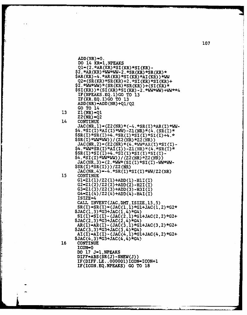
107

ADD (NR) -0.DO 14 KR-1,NPEAKSQi- (2. *AR(KR) *SI (KR) *SI (KR) -$2. *AR(KR)*WW*W..2 *SR(K)*SR(JR)*$AR(KR) -4.*AR(KR)*SI(KR)*AI(KR) )*WWQ2=(SR(KR)*SR(KR)+2 .*SI(KR)*SI(KR)+$2. *WW*W)*(SR(KR)*SR(R) )+(SI (KR)*$SI (KR) )*(SI(KR)*SI(yR)..*W*WW)+WW**4IF(NPEAKS.EQ.1)GO TO 13IF(K.R.EQ.I)GO TO 13ADD (NR) -ADD (NR)+Ql/Q2GO TO 14

13 Z1(NR)-QlZ2(NR) -Q2

14 CONTINUEJAC(NR, 1)=(Z2(NR)*(-4.*SR(I)*AR(I)*WW-$4.*SI(I)*AI (I)*WW)..Z1(NR)*(4 (SR(I)*$SR(I)*SR(I)+4. *SR(I)*SI (I)*SI (I)+4 .*$SR(I)*WW*WW) ) /(Z2 (NR)*Z2 (NR))JAC(NR,2)=(Z2(NR)*(4.*WW*AR(I)*SI(I)-$4.*W*SR(I)*AI(I)) -Z1(NR)*(4.*SR(I)*$SR(I)*SI(I)+4.*SI(I)*SI(I)*SI(I) -$4.*SI(I)*W*WWL))/ (Z2(NR)*Z2(NR))JAC(NR, 3)=(2 *W*(SI(I)*SI(I)-WW*WW-$SR(I)*SR(I) ) )/Z2(NR)JAC(NR, 4)=-4 .*SR(I)*SI(I)*WW/Z2(NR)

15 CONTINUEG1=Z (1) /Z2 (1)+ADD(1) -HlI (I)G2=Z1 (2) /Z2 (2)+ADD(2) -H21(I)G3=Z1(3) /Z2(3)+ADD(3) -H3I(I)G4-Z1(4) /Z2 (4)+ADD(4) -H41(I)ISIZE-4CALL INVERT(JAC,DMT,ISIZE,15,5)SR(I)-SR(I)-(JAC(11)*Gl+JAC(1,2)*G2*$JAC(1, 3)*G3+JAC(1,4)*G4)SI(I)-SI(I) -(JAC(2, 1)*GI+JAC(2, 2)*G2+$JAC (2, 3)*G3+JAC (2, 4)*G4)AR(I)-AR(I) -(JAG (3, 1)*G1+JAC (3, 2)*G2+$JAC(3, 3)*G3+JAC(3,4)*G4)AI(I)-AI(I) -(JAC(4, 1)*Gl+JAC(4, 2)*G2+$JAC (4, 3)*G3+JAC(4,4)*G4)

16 CONTINUEICON-ODO 17 J-1,NPEAKSDIFF-ABS (SR(J) -SNEW(J))IF (DIFF .LE. .000001) ICON-ICON+1IF(ICON.EQ.NPEAKS) GO TO 18

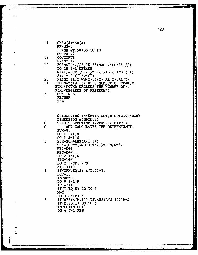
108

17 SNEW(J)-SR(J)NN-NN+1IF(NN.GT.50)GO TO 18GO TO 12

18 CONTINUEPRINT 19

19 FORMAT(/////,3X,*FINAL VALUES*,//)DO 20 I-1,NPEAKS

Z(I)--SR(I) /WN(I)20 PRINT 11,I,WN(I),Z(I),AR(I),AI(I)21 FORMAT(1Hl,3X,*THE NUMBER OF PEAKCS*,

$IX,*FOUND EXCEEDS THE NUMBER OF*,$1X,*DEGREES OF FREEDOM*)

22 CONTINUERETURNEND

SUBROUTINE INVERT, DET ,N ,NDIGIT ,NDIM)DIMENSION A(NDIM,8)

C THIS SUBROUTINE INVERTS A MATRIXC AND CALCULATES THE DETERMINANT.

SUH-O.DO 1 I=1,NDO 1 J-1,N

1 SUM=SUM+ABS(A(I,J))SUM-10. ** (-NDIGIT/ 2. )*SUM/N**2NP1=N+1NPN-N+NDO 2 I=1,NIPN- 1+NDO 2 J-NP1,NPNA(I,J)-0.

2 IF(IPN.EQ.J) A(I,J)=1.DET-1.INTCH-ODO 9 I-1,NIP1-I+1IF(I.EQ.N) GO TO 5M-IDO 3 J-IP1,N

3 IF(ABS(A(M, I)) .LT.ABS(A(J,I)))M-JIF(M.EQ.I) GO TO 5INTCH-INTCH+lDO 4 J-1,NPN

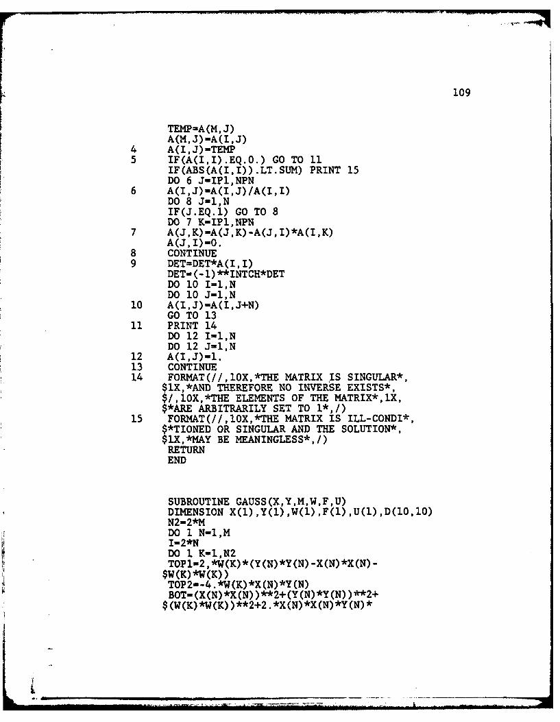
[109TEMP-A(M, J)A(4, J) -A (I, )

4 A(I,J)-TEMP5 IF(A(I,I).EQ.0.) GO TO 11

IF(ABS(A(I,I)).LT.SUM) PRINT 15DO 6 J-IP1,NPN

6 A(I,J)-A(IJ)/A(lII)DO 8 J-1,NIF (J. EQ. 1) GO TO 8DO 7 K-IP1,NPN

7 A(J,K)-A(J,K)-A(J,I)*A(I,K)A(J,I)=O.

8 CONTINUE9 DET=DET*A(I,I)

DET- (-1) **INTCH*DETDO 10 I=1,NDO 10 J-1,N

10 A(IJ)=A(IJ+N)GO TO 13

11 PRINT 14DO 12 1-1,NDO 12 J-1,N

12 A(I,J)-1.13 CONTINUE14 FORMAT(//,1OX,*THE MATRIX IS SINGULAR*,

$1X,*AND THEREFORE NO INVERSE EXISTS*,$/,1OX,*THE ELEMENTS OF THE MATRIX*,1X,$*ARE ARBITRARILY SET TO 1*,/)

15 FOR}IAT(//,1OX,*THE MATRIX IS ILL-CONDI*,$*TIONED OR SINGULAR AND THE SOLUTION*,$1X,*MAY BE MEANINGLESS*,/)RETURNEN])

SUBROUTINE GAUSS(X,Y,M,W,F,U)DIMENSION X(1) ,Y(1) ,W(1) ,F(1) ,U(1) ,D(1O,10)N2-2*MDO 1 N-1,MI-2*NDO 1 K-l,N2TOP1I.2,*W(K)*(Y(N)*Y(N) -X(N)*X(N)-$W(K)*W(K))TOP2--4 *W(K)*X(N)*Y (N)BOT=(X(N)*X(N) )**2+(Y(N)*Y(N) )**2+

$ (W(1)*W(K))**2+2 .*X(N)*X(N)*Y(N)*

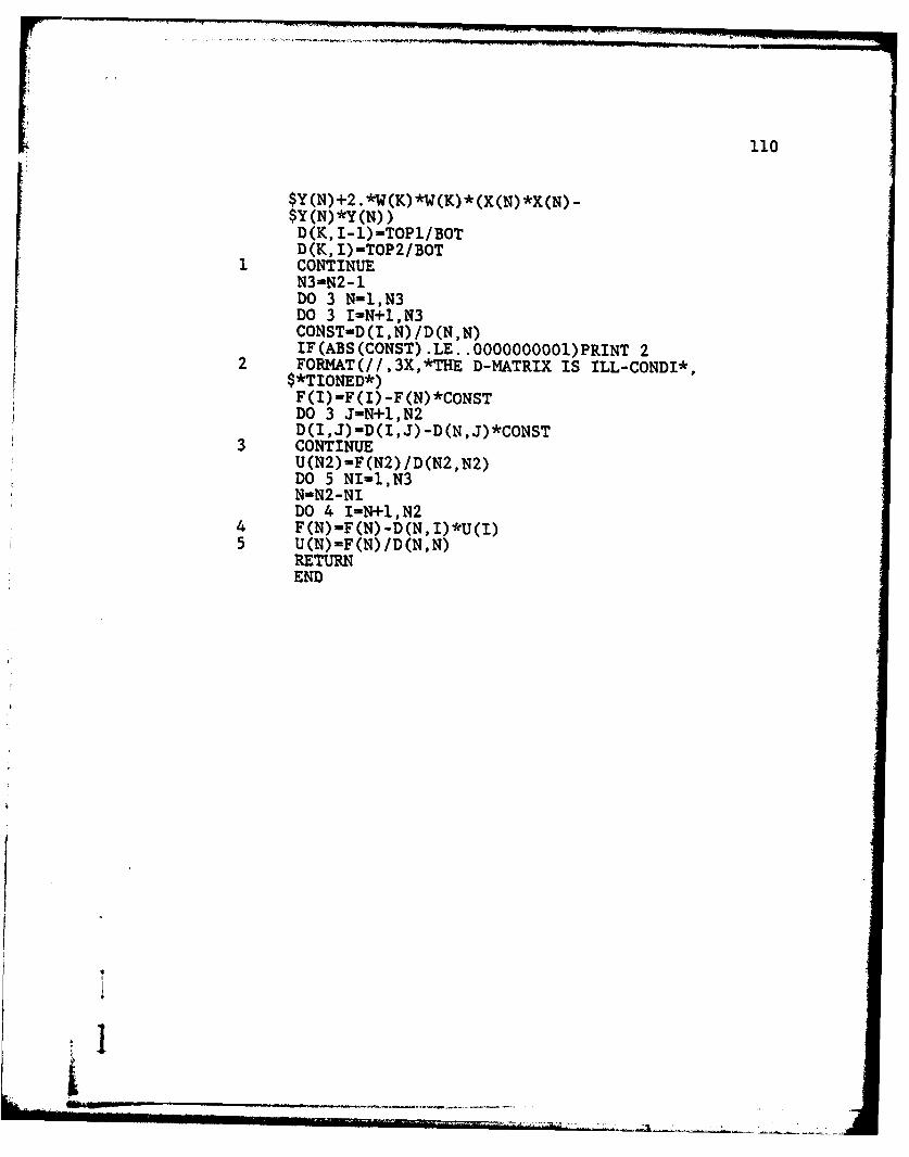
110

$Y(N)+2.*W(K)*W(K)*(X(N)*X(N) -$Y(N)*Y(N))D(K, I-1) -TOPl/BOTrD (K, I) -TOP 2/ BOT

1 CONTINUEN3-N2- 1DO 3 N-1,N3DO 3 I-N+1,N3CONST-D(I,N) /D(N,N)IF(ABS(CONST) .LE. .O000000001)PRINT 2

2 FORMAT(//,3X,*THE D-MATRIX IS ILL-CONDI*,$*TIONED*)F(l)-F(I) -F(N)*CONSTDO 3 J-N+1,N2D(I,J)-D(I,J) -D(N,J)*CONST

3 CONTINUEU(N2)-F(N2)/D(N2,N2)DO 5 NI-1,N3N-N2-NIDO 4 I-N+1,N2

4 F(N)-FCN)-D(N,I)*U(I)5 U(N)-F(N)/D(N,N)

RETURNEND

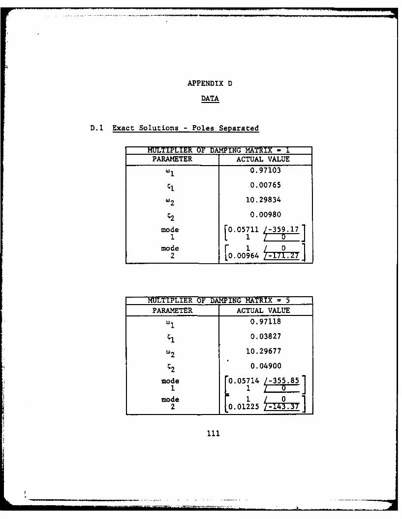
APPENDIX D

DATA

D.1 Exact Solutions - Poles Separated

MULTIPLIER OF DAMPING MATRIX - IPARAMETER ACTUAL VALUE

W1 0.97103

c1 0.00765

w2 10.29834

C2 0.00980

mode [0.05711 J3917]

mode1

______o_______[o 0o 4_ B!o 2!]2 .0. 00964 Tr

MULTIPLIER OF DAMPING MATRIX = 5

PARAMETER ACTUAL VALUE

w1 0.97118

0.03827

-w2 10.29677

C2 0.04900

mode 0.05714 /-355.851 [ 1U1 - 0

mode 1 Lf~2 0.01225

111

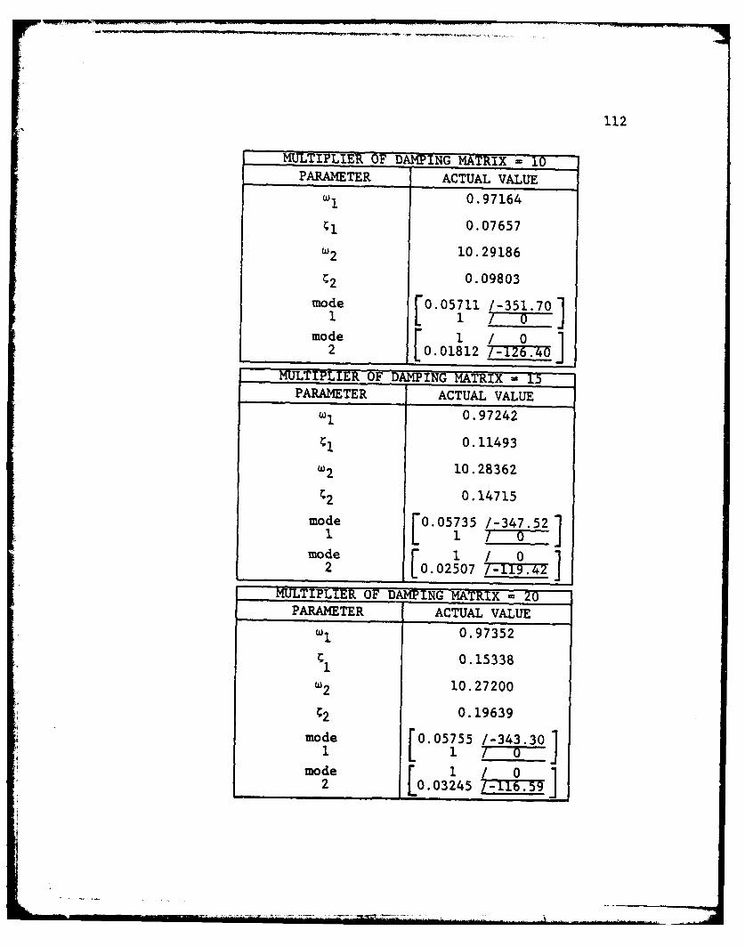
112

MULTIPLIER OF DAMPING MATRIX = 10PARAMETER ACTUAL VALUE

wI 0.97164

I 0.07657

w2 10.29186

2 0.09803

mode F0.05711 /-351.7011 1L7 _

mode 1 10 12 L0-01812 7 126.40

MULTIPLIER OF DAMPING MATRIX = 15PARAMETER ACTUAL VALUE

Wi 0.97242

i 0.11493

w2 10.28362

2 0.14715

mode F0.05735 /-347.521 L0~T

mode 0 1012 0.02 507 7-119.42

MULTIPLIER OF DAMPING MATRIX - 20PARAMETER ACTUAL VALUE

W1 0.97352

; 1 0.15338

w2 10.27200

02 0.19639

mode 0.05755 /-343.30,1 _

mode02 [0.03245 7- M-57.!_ _ _ _ _

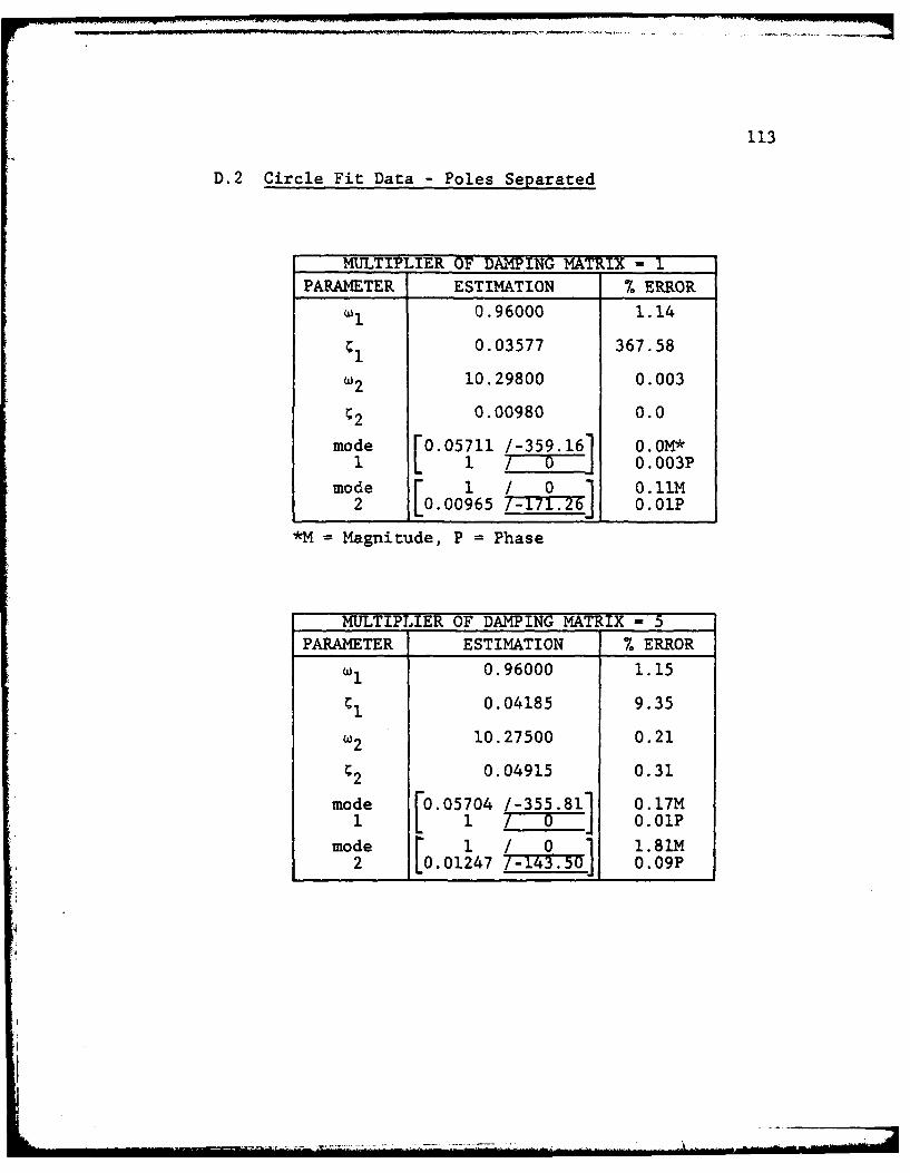
113

D.2 Circle Fit Data - Poles Separated

MULTIPLIER OF DAMPING MATRIX I

PARAMETER ESTIMATION % ERROR

0.96000 1.14

0.03577 367.58

w2 10.29800 0.003

2 0.00980 0.0

mode [0.05711 /-359.16 0.OM*1 L 1 0 0.003P

mode 1 /0 0.11M2 10.00965 0.01P

*M Magnitude, P = Phase

MULTIPLIER OF DAMPING MATRIX = 5PARAMETER ESTIMATION % ERROR

Wi 0.96000 1.15

c 0.04185 9.35

w2 10.27500 0.21

C2 0.04915 0.31

mode [0.05704 /-355.81] .17M1 1 0 0.01P

mode 1 / 0 1.81M2 .0.01247 /-143.50 0.09P

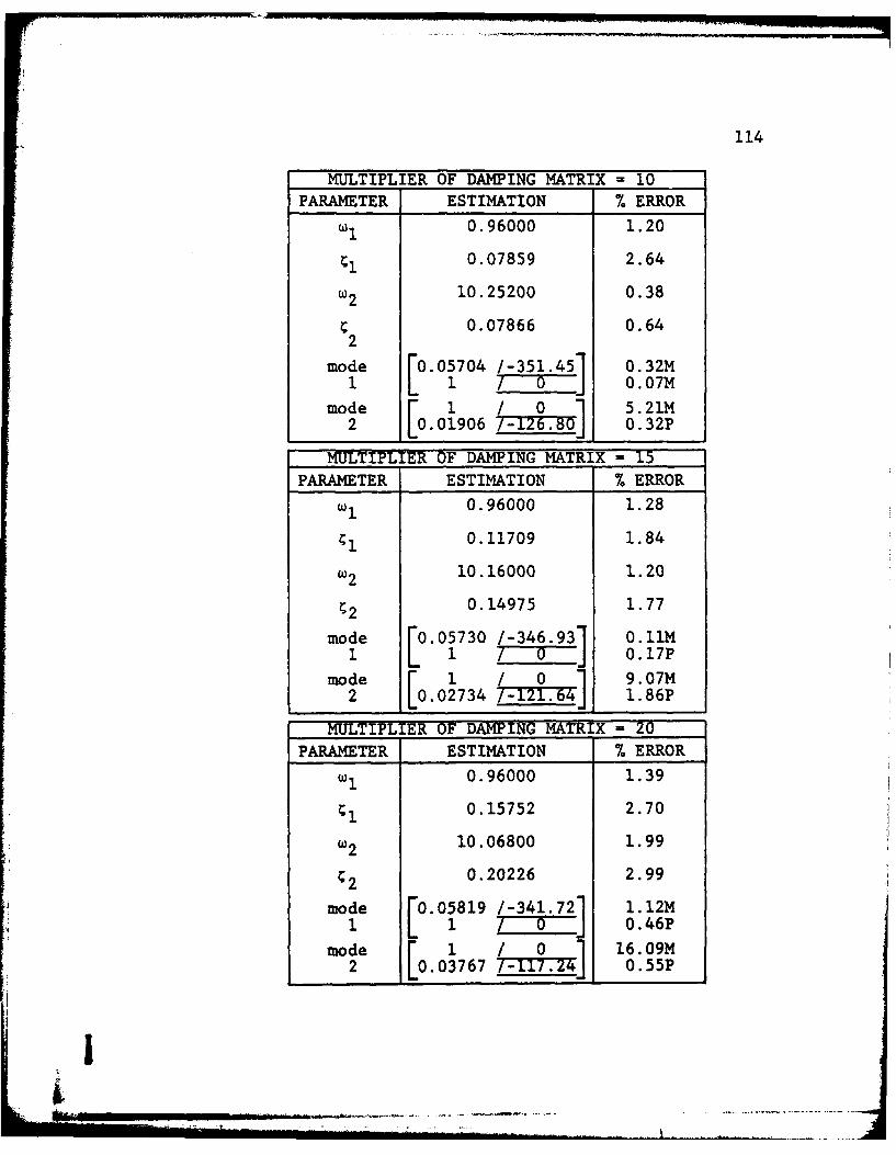
114

MULTIPLIER OF DAMPING MATRIX = 10PARAMETER ESTIMATION % ERROR

WI 0.96000 1.20

C1 0.07859 2.64

W2 10.25200 0.38

0.07866 0.642

mode [0.05704 /-351.451 0.32M1 1 0 .07M

mode 1 / 0 1 5.21M2 [0.01906 /-126.8 0.32P

MULTIPLIER OF DAMPING MATRIX 15PARAMETER ESTIMATION % ERROR

Wi 0.96000 1.28

0.11709 1.84

10.16000 1.20

2 0.14975 1.77

mode F0.05730 /-346.931 0.11MI 1 0 j 0.17P

mode / 0 1 9.07M2 0. 0 2 7 34 /-2TT7.4 1.86P

MULTIPLIER OF DAMPING MATRIX 20

PARAMETER ESTIMATION % ERROR

WI 0.96000 1.39

;1 0.15752 2.70

w2 10.06800 1.99

C2 0.20226 2.99

mode "0.05819 /-341.721 1.12M1 1 I _0 0.46P

mode r 1 / 0 1 16.09M2 0.03767 0 0.55P

I

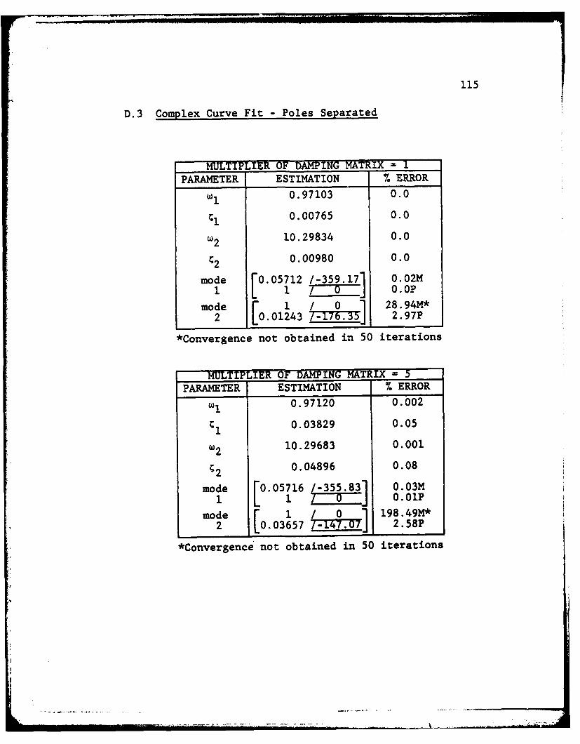
115

D.3 Complex Curve Fit - Poles Separated

MULTIPLIER OF DAMPING M-ATRIX - I

PARAMETER ESTIMATION % ERROR

Wi 0.97103 0.0

r;1 0.00765 0.0

w2 10.29834 0.0

C2 0.00980 0.0

mode [0.05712 /-359.17] 0.02M1____1 0.0?

mode l 01 28.94M*2 0. 0 1 2 43 71735] 2.97P

*Convergence not obtained in 50 iterations

MULTIPLIER OF DAMPING ATRIX - 5PARAMETER ESTIMATION % ERROR

W1 0.97120 0.002

C 0.03829 0.05

w2 10.29683 0.001

2 .04896 0.08

mode L05716 /-558 0.03Mmode 1 0 1198.49M*

2____ L0. 03657 7-747.07J 2.58P

*Convergence not obtained in 50 iterations

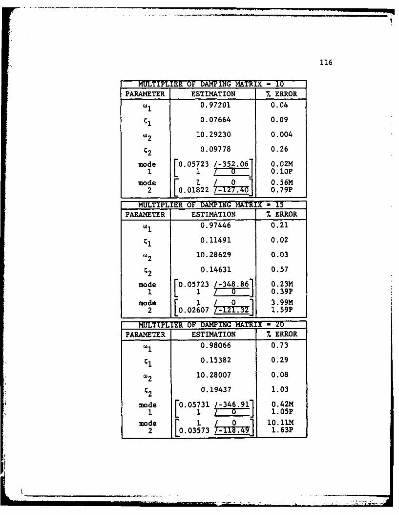
116

MULTIPLIER OF DAMPING MATRIX - 10

PARAMETER ESTIMATION 7. ERROR

Wi 0.97201 0.04

CI 0.07664 0.09

W2 10.29230 0.004

C2 0.09778 0.26

mode 0.05723 /-352.06 0.02M1 L i o 0.1op

mode 1 / 0 1 0.56M2 L0 .01822 T.27.40 0.79P

MULTIPLIER OF DAMPING MATRIX 15

PARAMETER ESTIMATION % ERROR

W1 0.97446 0.21

Ci 0.11491 0.02

wi2 10.28629 0.03

2 .14631 0.57

mode F0.05723 /-348.861 0.23M1 1 7 o 0.39P

mode I / 0 1 3.99M2 L0.0 2 60 7 /-12.32 1.59P

MULTIPLIER OF DAMPING MATRIX 20PARAMETER ESTIMATION 7 ERROR

W1 0.98066 0.73

€I 0.15382 0.29

w2 10.28007 0.08

C2 0.19437 1.03

mode F0.05731 /-346.911 0.42M1 L1 T~J 1.05p

mode F0 o/ 0 10.1iM2 0.03573 I-18.49 1.63P

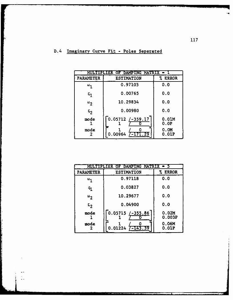
117

D.4 Imaginary Curve Fit - Poles Separated

MULTIPLIER OF DAMPING MATRIX = 1PARAMETER ESTIMATION % ERROR

w1 0.97103 0.0

C1 0.00765 0.0

w2 10.29834 0.0

;2 0.00980 0.0

mode 05712 /-359.17 O.O1M1 1 0 o ooP

mode 1 0 1 0.0M2 .00964 /71.291 0.01P

MULTIPLIER OF DAMPING MATRIX - 5

PARAMETER ESTIMATION % ERROR

Wi 0.97118 0.0

0.03827 0.0

w2 10.29677 0.0

;2 0.04900 0.0

mode O.05715 /-355.861 0.02M1 1 7 J 0.003P

mode [O 1 /0 006M2 .01224 1433 0.01P

10

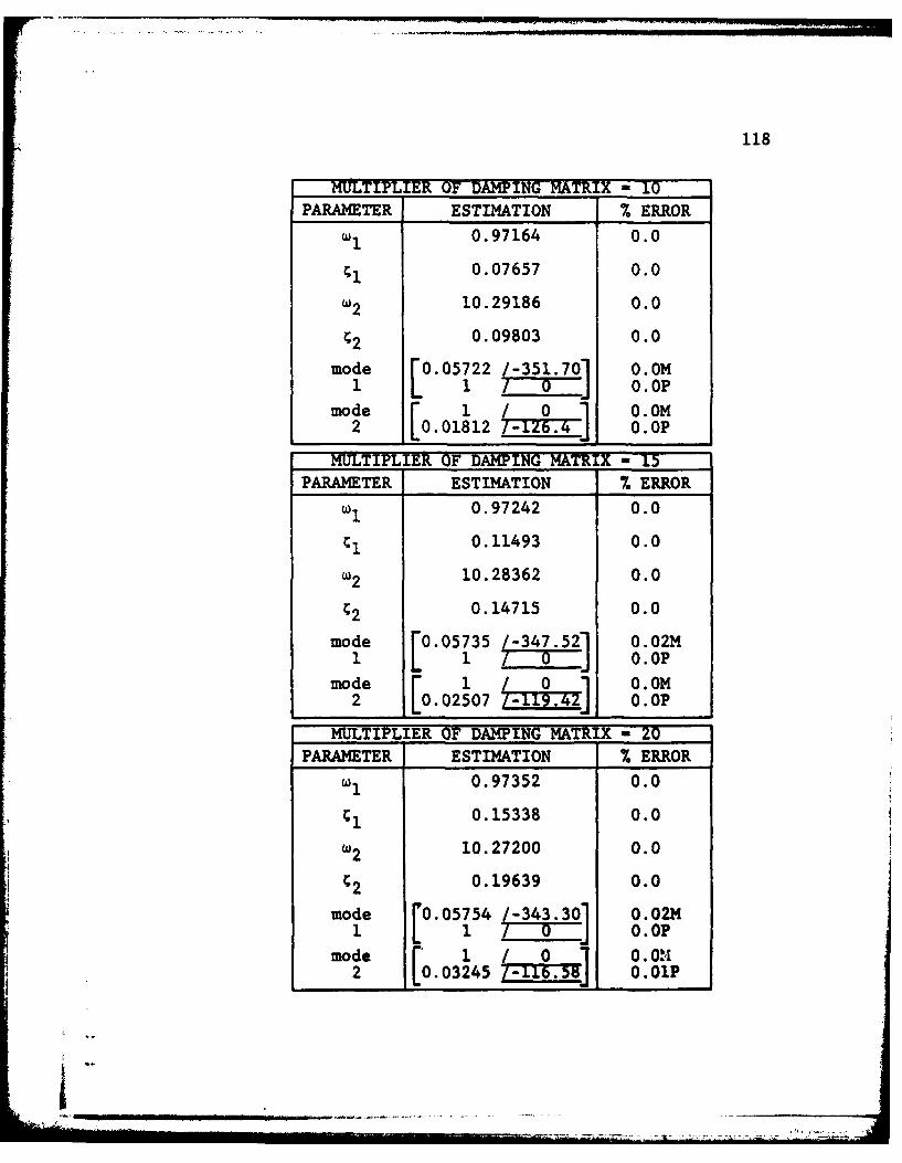
118

MULTIPLIER OF DAMPING MATRIX - 10PARAMETER ESTIMATION 7 ERROR

w 0.97164 0.0

CI 0.07657 0.0

w2 10.29186 0.0

C2 0.09803 0.0

mode r0.05722 /-351.701 0.0M1 L 1 0TJ 0. OP

mode 1 / 0 1 0.OM2 0. 0 18 12 /-12b.4 0.0P

-TIPLER OF DAMPING MATR- 5PARAMETER ESTIMATION 7. ERROR

w 0.97242 0.0

Ci 0.11493 0.0

2 0.28362 0.0

C2 0.14715 0.0

mode F0.05735 /-347.521 0.02M1 L 1 0T 0. OP

mode - 1 / 0 1 0.0M2 0.02507 Ti-.J 0.0P

MULTIPLIER OF DAMPING MATRIX - 20PARAMETER ESTIMATION 7. ERROR

WI 0.97352 0.0

ci 0.15338 0.0

w2 10.27200 0.0

¢2 0.19639 0.0

mode r0.05754 /-343.301 0.02M1 L L~ j 0.0 OP

mode 1 ~ ,v, 02 .03 24 5 0.

.... .... .... _....__ ___1__ __-___"

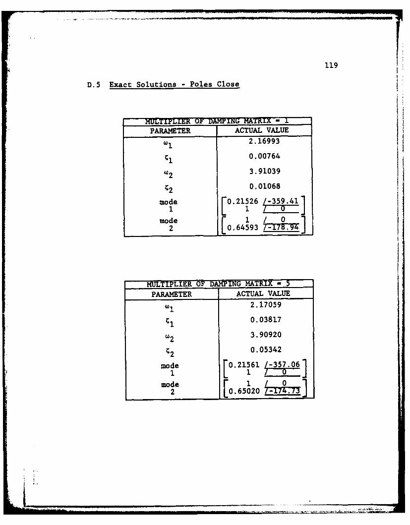
119

D.5 Exact Solutions - Poles Close

MULTIPLIER OF DAMPING MATRIX - 1

PARAMETER ACTUAL VALUE

Wi 2.16993

0.00764

w2 3.91039

C2 0.01068

mode [0.21526 /-359.41]•1L 1 7 -omode1

2 O.64593

MULTIPLIER OF DAMPING MATRIX " 5

PARAMETER ACTUAL VALUE

(I 2.17059

0.03817

w2 3.90920

C2 0.05342

mode "0.21561 /-357.061 7mode 0

_____ _2 __ [0.65020 Il~

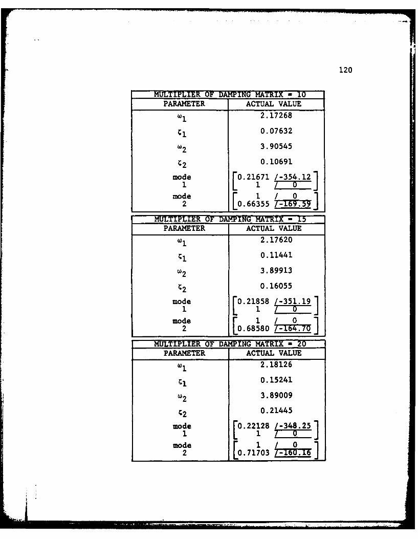
120

MULTIPLIER OF DAMPING MATRIX - 10PARAMETER ACTUAL VALUE

Wi 2.17268

€ 1 0.07632

W2 3.90545

r.2 0.10691

mode 0.21671 /-354.12

mode102 0.66355 T6TT

MULTIPLIER OF DAMPING MATRIX - 15PARAMETER ACTUAL VALUE

W1 2.17620

1 0.11441

w2 3.89913

0.16055

mode 0.21858 /-351.19

mode102 10 .68580

MULTIPLIER OF-DAMPING MATRIX - 20

PARAMETER ACTUAL VALUE

Wi 2.18126

0.15241

w2 3.89009

42 0.21445

mode 0.22128 -348.251 1 10

mode12 _0._71703-_.[o.

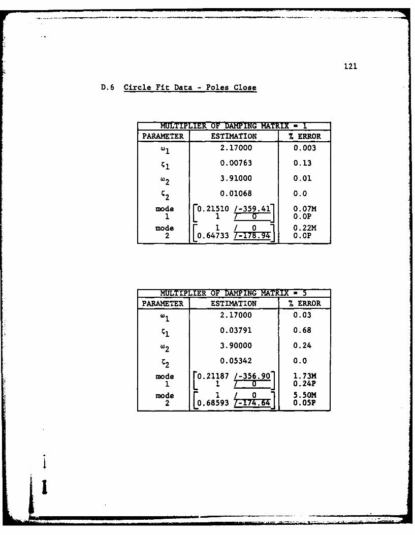
121

D.6 Circle Fit Data - Poles Close

MULTIPLIER OF DAMPING MATRIX - 1PARAMETER ESTIMATION % ERROR

WI 2.17000 0.003

€1 0.00763 0.13

w2 3.91000 0.01

c2 0.01068 0.0

mode F0"21510 /-359.41" 0.07M1 P. 1 0 ] 0. OP

mode l /01 0.22M2 L 0 . 64 73 3 0.0P

MULTIPLIER OF DAMPING MATRIX - 5PARAMETER ESTIMATION 7. ERROR

(1) 2.17000 0.03

0.03791 0.68

w2 3.90000 0.24

2 0.05342 0.0

mode 0.21187 /-356.90 1.73M1 1 TUJ 0.24P

mode 1 0855. /0]M2 0 68593 L ,146 0.05P

i1

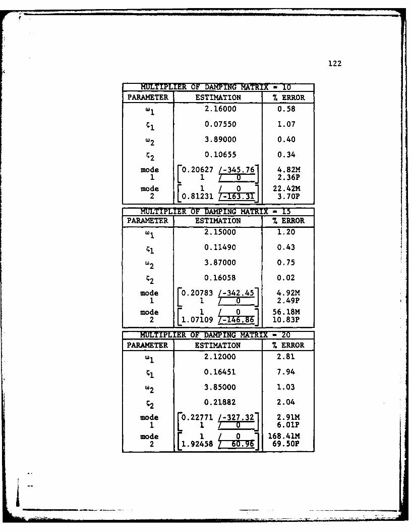
122

MULTIPLIER OF DAMPING MATRIX - 10PARAMETER ESTIMATION 7. ERROR

i 2.16000 0.58

Ci 0.07550 1.07

W2 3.89000 0.40

2 0.10655 0.34

mode FO.20627 /-345.761 4.82M1 L 1 0 2.36P

mode F 1 / 01 22.42M2 0.81231 L-163.31 3.70P

MULTIPLIER OF DAMPING MATRIX - 15PARAMETER ESTIMATION 7 ERROR

Wi 2.15000 1.20

ri 0.11490 0.43

w2 3.87000 0.75

2 .16058 0.02

mode FO.20783 /-342.451 4.92M1 L 1 / 0o 2.49P

mode i 1 / 01 56.18M2 1 *07109 -146.861 10.83P

MULTIPLIER OF DAMPING MATRIX - 20PARAMETER ESTIMATION 7 ERROR

WI 2.12000 2.81

;i 0.16451 7.94

u2 3.85000 1.03

C2 0.21882 2.04

mode [0.22771 /2.21 2.91M

mode 1 06 168.41M2 Ill.92458 60.96J 69.50P

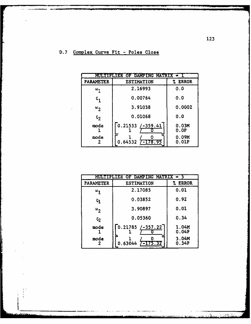
123

D.7 Complex Curve Fit - Poles Close

MULTIPLIER OF DAMPING MATRIX - 1PARAMETER ESTIMATION % ERROR

WI 2.16993 0.0

cI 0.00764 0.0

W2 3.91038 0.0002

2 0.01068 0.0

mode F"0 21533 /-359.411 O.03M1 L~ 0.0 OP

mode F 1 / 0 1 0.09m2 L0.64532 Th178.95 0.01P

MULTIPLIER OF DAMPING MATRIX = 5PARAMETER ESTIMATION % ERROR

WI 2.17085 0.01

Ci 0.03852 0.92

w2 3.90897 0.01

0.05360 0.34

mode F.21785 /-357.22 1.04M1 L 1 0____ 0. 04P

mode F 1 0 1 3.04M2 0.63044 7hT73= 0.34P

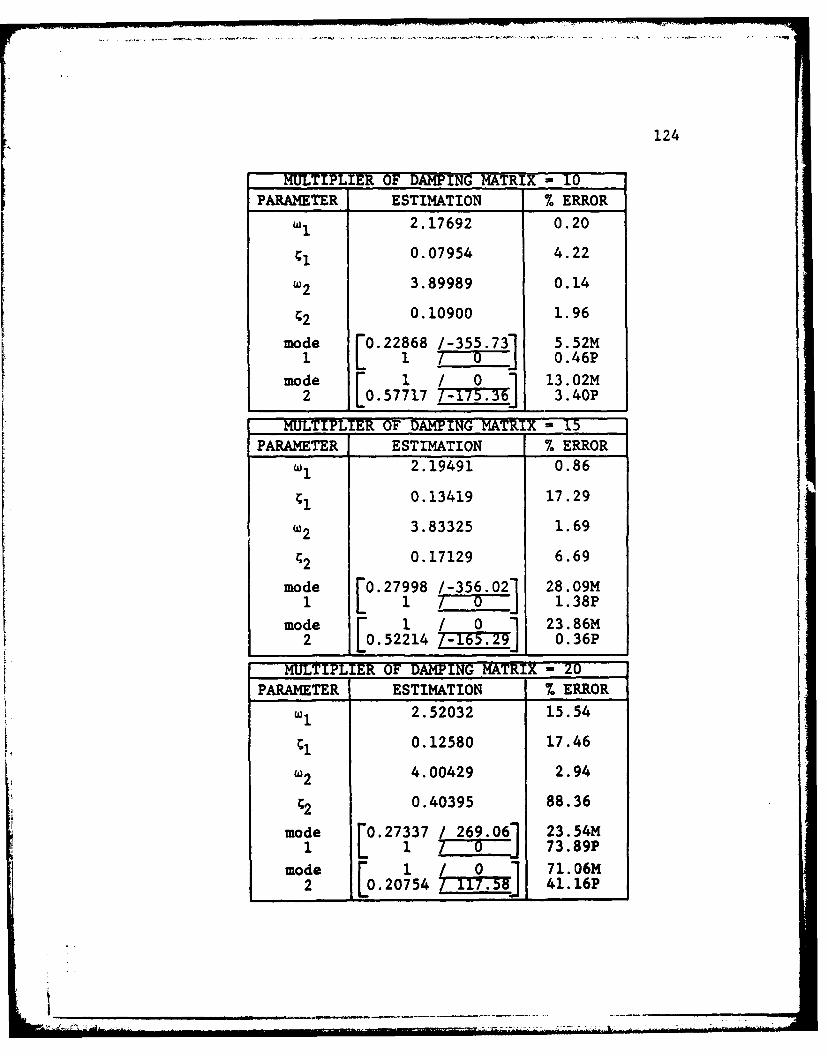
124

MULTIPLIER OF DAMPING MATRIX - 10PARAMETER ESTIMATION % ERROR

Wi 2.17692 0.20

Cl1 0.07954 4.22

w2 3.89989 0.14

C2 0.10900 1.96

mode F0.22868 /-355.731 5.52M1 L i WJ 0.46P

mode 1 0 13.02M2 L 1057717 Ld=- 3.40P

MULTIPLIER OF DAMPING MATRIX - 15

PARAMETER ESTIMATION 7. ERROR

WI 2.19491 0.86

41 0.13419 17.29

w2 3.83325 1.69

C2 0.17129 6.69

mode F0"27998 /-356.021 28.09M1 L 1 T ]0 1.38P

mode F 1 / 0 1 23.86M2 0.52214 -165.9. 0.36P

MULTIPLIER OF DAMPING MATRIX 20PARAMETER ESTIMATION % ERROR

W1 2.52032 15.54

C1 0.12580 17.46

w2 4.00429 2.94

C2 0.40395 88.36

mode L0 .27337 /269.06 23.54M

mode Fl 1 Q 71.06M42 0.20754 41.16P

41.16___ __ __ __ __ _ __

125

D.8 Imaginary Curve Fit - Poles Close

MULTIPLIER OF DAMPING MATRIX = 1PARAMETER ESTIMATION 7. ERROR

Wi 2.16994 0.0004

I 0.00754 1.29

w2 3.91038 0.0003

C2 0.01031 3.50

mode [0.21535 /-359.37 0.04M1 1 7 0 ._ 0.01P

mode [ 1 0 0.002M2 L0. 64594 7I17 0.04P

MULTIPLIER OF DAMPING MATRIX - 5PARAMETER ESTIMATION 7 ERROR

Wi 2.17069 0.005

I 0.03770 1.22

a2 3.90902 0.004

2 0.05154 3.51

mode [0.21563 /-356.87 0.01M1_1_7___0 0.05P

mode 0 1 / 0 0.04M2 L0 .65047 T 4 0.20P

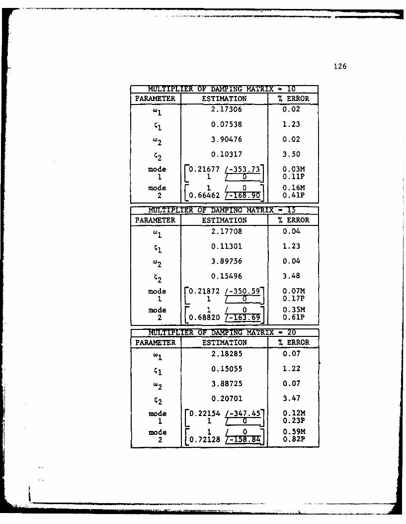
126

MULTIPLIER OF DAMPING MATRIX = 10PARAMETER ESTIMATION 7. ERROR

Wi 2.17306 0.02

I 0.07538 1.23

w2 3.90476 0.02

2 0.10317 3.50

mode j0"21677 /-353.73 0.03M

mode 1o i / 0 0.16M2 0.66462 /-6.0 0.41P I

MULTIPLIER OF DAMPING MATRIX 15

PARAMETER ESTIMATION % ERROR

to 2.17708 0.04

CI 0.11301 1.23

w2 3.89756 0.04

2 .15496 3.48

mode FO.21872 /-350.591 O.07M1 L 1 /__0 o.17P

mode [ 1 /0 .35M2 L10 .68820 /-6.9 0.61P

MULIPERO DAMPING MATRIX 20

PARAMETER ESTIMATION % ERROR

Wi 2.18285 0.07

1i 0.15055 1.22

3.88725 0.07

*2 0.20701 3.47

mode F0.22154 /-347.45 0.12M1 L 1 7 -__ 0.23P

mode 1 004 .59M2 .72128 /-158.8 0.82P

-.L .

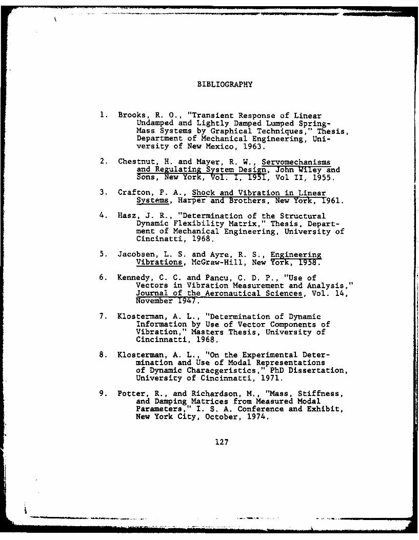
BIBLIOGRAPHY

1. Brooks, R. 0., "Transient Response of LinearUndamped and Lightly Damped Lumped Spring-Mass Systems by Graphical Techniques," Thesis,Department of Mechanical Engineering, Uni-versity of New Mexico, 1963.

2. Chestnut, H. and Mayer, R. W., Servomechanismsand Regulating System Design, John Wiley andSons, New York, Vol. I, 1951, Vol II, 1955.

3. Crafton, P. A., Shock and Vibration in LinearSystems, Harper and Brothers, New York, 1961.

4. Hasz, J. R., "Determination of the StructuralDynamic Flexibility Matrix," Thesis, Depart-ment of Mechanical Engineering, University ofCincinatti, 1968.

5. Jacobsen, L. S. and Ayre, R. S., EngineeringVibrations, McGraw-Hill, New York, 1958.

6. Kennedy, C. C. and Pancu, C. D. P., "Use ofVectors in Vibration Measurement and Analysis,"Journal of the Aeronautical Sciences, Vol. 14,November 1947.

7. Klosterman, A. L., "Determination of DynamicInformation by Use of Vector Components ofVibration," Masters Thesis, University ofCincinnatti, 1968.

8. Klosterman, A. L., "On the Experimental Deter-mination and Use of Modal Representationsof Dynamic Characgeristics," PhD Dissertation,University of Cincinnatti, 1971.

9. Potter, R., and Richardson, M., "Mass, Stiffness,and Damping Matrices from Measured ModalParameters," I. S. A. Conference and Exhibit,New York City, October, 1974.

127

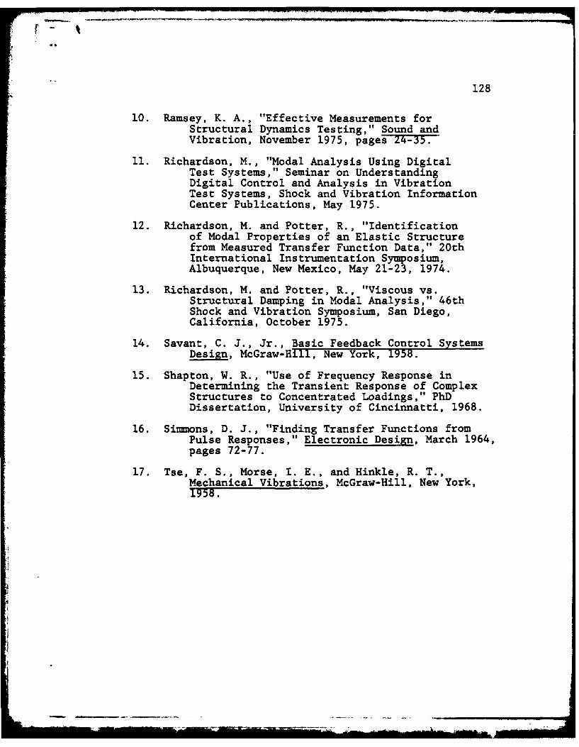
128

10. Ramsey, K. A., "Effective Measurements forStructural Dynamics Testing," Sound andVibration, November 1975, pages 24-35.

11. Richardson, M., "Modal Analysis Using DigitalTest Systems," Seminar on UnderstandingDigital Control and Analysis in VibrationTest Systems, Shock and Vibration InformationCenter Publications, May 1975.

12. Richardson, M. and Potter, R., "Identificationof Modal Properties of an Elastic Structurefrom Measured Transfer Function Data," 20thInternational Instrumentation Symposium,Albuquerque, New Mexico, May 21-23, 1974.

13. Richardson, M. and Potter, R., "Viscous vs.Structural Damping in Modal Analysis," 46thShock and Vibration Symposium, San Diego,California, October 1975.

14. Savant, C. J., Jr., Basic Feedback Control SystemsDesign, McGraw-Hill, New York, 1958.

15. Shapton, W. R., "Use of Frequency Response inDetermining the Transient Response of ComplexStructures to Concentrated Loadings," PhDDissertation, University of Cincinnatti, 1968.

16. Simmons, D. J., "Finding Transfer Functions fromPulse Responses," Electronic Design, March 1964,pages 72-77.

17. Tse, F. S., Morse, I. E., and Hinkle, R. T.,Mechanical Vibrations, McGraw-Hill, New York,1958.

VITA

Clarence Walter Miller was born in North

Charleroi, Pennsylvania, on March 14, 1947, the son

of Mulford J. Miller (deceased), and Clara C. Miller.

After graduation from Charleroi Area Senior High School,

Charleroi, Pennsylvania, in 1965, he entered LeTourneau

College in Longview, Texas. Upon completion of the

Aviation Technician Program at LeTourneau, he entered

the United States Air Force in 1968. In 1971, under

the Air Force Airman Education and Commissioning Pro-

gram, he entered the University of Texas at Austin.

He received his Bachelor of Science in Aerospace En-

gineering from the University of Texas in 1973. In

September, 1977, he entered the Graduate School of the

University of Texas under another Air Force education

program.

Permanent Address: 815 ParkviewKilgore, Texas 75662

This Thesis was typed by Vickie Lynn Miller.

K_______________