Embed Size (px)
Citation preview

Horizon 2020 - LCE-2017 - SGS
FLEXCoop
Democratizing energy markets through the introduction of innovative
flexibility-based demand response tools and novel business and market models
for energy cooperatives
WP2 - STAKEHOLDERS REQUIREMENTS, BUSINESS MODELS AND
ARCHITECTURE DESIGN
D2.5 – FLEXCoop PMV Methodology
Specifications – Preliminary Version
Due date: 30.09.2018 Delivery Date: 29.10.2018
Author(s): Andrea Conserva (CIRCE), Juan Aranda (CIRCE), Laura Morcillo (ETRa), Armin
Ghasem Azar (DTU), Roland Tual (RESCoop)
Editor: Andrea Conserva (CIRCE)
Lead Beneficiary of Deliverable: CIRCE
Dissemination level: Public Nature of the Deliverable: Report
Internal Reviewers: Hrvoje Keko (Koncar), Christos Malavazos (Grindrop), Katarina
Valalaki (Hypertech), Silke Cuno (Fraunhofer)

HORIZON 2020 –773909 - FLEXCoop D2.5 – FLEXCoop PMV Methodology Specifications
– Preliminary Version
WP2 – Stakeholders Requirements, Business Models and Architecture Design FLEXCoop Consortium
Page 2 of 75
FLEXCOOP KEY FACTS
Topic: LCE-2016-2017 – Next generation innovative technologies enabling
smart grids, storage and energy system integration with increasing
share of renewables: distribution network.
Type of Action: Research and Innovation Action
Project start: 01 October 2017
Duration: 36 months from 01.10.2017 to 30.09.2020 (Article 3 GA)
Project Coordinator: Fraunhofer
Consortium: 13 organizations from nine EU member states
FLEXCOOP CONSORTIUM PARTNERS
Fraunhofer Fraunhofer-Gesellschaft zur Förderung der angewandten Forschung e.V.
ETRa ETRA INVESTIGACION Y DESARROLLO SA
HYPERTECH HYPERTECH (CHAIPERTEK) ANONYMOS VIOMICHANIKI
DTU DANMARKS TEKNISKE UNIVERSITET
GRINDROP GRINDROP LIMITED
CIRCE FUNDACION CIRCE CENTRO DE INVESTIGACION DE RECURSOS
Y CONSUMOS ENERGETICOS
KONCAR KONCAR - INZENJERING ZA ENERGETIKUI TRANSPORT DD
SUITE5 SUITE5 DATA INTELLIGENCE SOLUTIONS Limited
S5 SUITE5 DATA INTELLIGENCE SOLUTIONS Limited
CIMNE CENTRE INTERNACIONAL DE METODES NUMERICS EN
ENGINYERIA
RESCOOP.EU RESCOOP EU ASBL
SomEnergia SOM ENERGIA SCCL
ODE ORGANISATIE VOOR HERNIEUWBARE ENERGIE DECENTRAAL
Escozon ESCOZON COOPERATIE UA - affiliated or linked to ODE
MERIT MERIT CONSULTING HOUSE SPRL
Disclaimer: FLEXCoop is a project co-funded by the European Commission under the Horizon
2020 – LCE - 2017 – SGS under Grant Agreement No. 773909.
The information and views set out in this publication are those of the author(s) and do not
necessarily reflect the official opinion of the European Communities. Neither the European
Union institutions and bodies nor any person acting on their behalf may be held responsible for
the use, which may be made of the information contained therein.
© Copyright in this document remains vested with the FLEXCoop Partners

HORIZON 2020 –773909 - FLEXCoop D2.5 – FLEXCoop PMV Methodology Specifications
– Preliminary Version
WP2 – Stakeholders Requirements, Business Models and Architecture Design FLEXCoop Consortium
Page 3 of 75
EXECUTIVE SUMMARY
The objective of this document, main outcome of the FLEXCoop Task 2.4 on “Definition of
Monitoring and Verification Methodology for DR settlement and remuneration and Key
Performance Indicators”, is to define the Performance Measurement and Verification
Methodology (PMV) to be adopted by the FLEXCoop project for verifying consumer response
rate to dispatched Demand Response (DR) signals. Existing approaches already developed in
other EU projects and in the international context have been considered for the definition of the
methodology. Thus, a literature research work has been carried out and is presented in the first
part of this document. Special attention has been given to the International Performance
Measurement and Verification Protocol (IPMVP) and Federal Energy Management Programme
(FEMP) protocols, the most used at international level for Measurement and Verification
(M&V) projects and to previous EU project such as eeMeasure, Moeebius, OrbEEt an
HOLISDER. Furthermore, an analysis of already existing baseline estimation methodologies
has been also carried out to identify the main barriers currently existing in M&V in DR. From
this basis, understanding how FLEXCoop PMV can address these barriers and its main
contribution to the current State-of-the-Art has been studied. As a result, considering that the
definition of the baseline resulted as the most crucial aspect in M&V in DR. The FLEXCoop
PMV adopts the FLEXCoop models (developed in FLEXCoop Work Package 3) to provide an
innovative approach to this challenge. The most common issues for baselining construction are
related to the selection of representative days as basis for estimation, setting of exclusion rules
to avoid considering non-representative consumption, definition of adjustments’ types and
windows. Thanks to the adoption of the FLEXCoop models, these aspects can be improved.
The models provide a continuously auto-calibrated baseline that uses data from the minimum
number of recent days needed to obtain a high accuracy. Furthermore, since FLEXCoop
solutions provide automated DR, the models will receive signals when electrical systems go
into preparation status (e.g. for pre-heating or pre-cooling) and will automatically exclude ramp
periods from the basis of estimations. The models will also provide forecasting of human
actions and occupancy, allowing the detection of manipulation’s attempts from the users. As
main result of this work, the PMV has been defined, taking also in consideration the most
common recommendations found for M&V in DR events. The methodology, composed by
three phases and three steps for each of them, has been defined as following:
1) Ex-ante analysis
a) Definition of DR events and criteria for remuneration.
b) Definition of DR systems and minimum comfort conditions
c) Identification of static and dynamic variables that affect the demand and need to be
measured.
2) Implementation
a) Analysis of existing monitoring system and specification of metering points and
sensors’ characteristics.
b) Analysis of the technical and economic reliability of individual loads measurements.
c) Conduct post-installation verification activities for algorithm calibration.
3) Ex-post analysis
a) Testing of the system in a DR event to validate model accuracy and reliability.
b) Demand reduction assessment
c) Definition of the PMV report

HORIZON 2020 –773909 - FLEXCoop D2.5 – FLEXCoop PMV Methodology Specifications
– Preliminary Version
WP2 – Stakeholders Requirements, Business Models and Architecture Design FLEXCoop Consortium
Page 4 of 75
Table of Contents
FLEXCOOP KEY FACTS ................................................................................................................................... 2
FLEXCOOP CONSORTIUM PARTNERS ....................................................................................................... 2
EXECUTIVE SUMMARY ................................................................................................................................... 3
LIST OF FIGURES .............................................................................................................................................. 6
LIST OF TABLES ................................................................................................................................................ 6
ABBREVIATIONS ............................................................................................................................................... 7
1. INTRODUCTION ............................................................................................................................................. 9
2. M&V OVERVIEW ........................................................................................................................................... 9
2.1. INTERNATIONAL PERFORMANCE MEASUREMENT AND VERIFICATION PROTOCOL (IPMVP) ...................... 12 2.2. FEMP......................................................................................................................................................... 16 2.3. ASHRAE GUIDELINE 14 ............................................................................................................................ 17 2.4. THE DOE UNIFORM METHODS PROJECT .................................................................................................... 17 2.5. M&V METHODOLOGIES USED FOR DR ASSESSMENT .................................................................................. 17
2.5.1. The eeMeasure methodology ............................................................................................................. 19 2.5.2. Other EU Projects ............................................................................................................................. 23
3. BASELINE ESTIMATION IN M&V METHODOLOGIES ...................................................................... 25
3.1. BASELINE ESTIMATION METHODS ............................................................................................................... 26 3.1.1. Maximum Base Load ......................................................................................................................... 26 3.1.2. Meter Before/Meter After .................................................................................................................. 26 3.1.3. Baseline Type I .................................................................................................................................. 27 3.1.4. Baseline Type II ................................................................................................................................. 28 3.1.5. Experimental design .......................................................................................................................... 28 3.1.6. Metering Generator Output ............................................................................................................... 30
3.2. EXPLORATORY DATA ANALYSIS ................................................................................................................. 30 3.2.1. Day matching ..................................................................................................................................... 30 3.2.2. Regression analysis ........................................................................................................................... 34
3.3. BASELINE ADJUSTMENTS ............................................................................................................................ 38 3.4. UNCERTAINTY ............................................................................................................................................ 40 3.5. APPLICATION OF BASELINE METHODOLOGIES............................................................................................. 42
3.5.1. California Energy Commission ......................................................................................................... 42 3.5.2. ERCOT Demand Side Working Group .............................................................................................. 42 3.5.3. Southern California Edison - Methods for Short-duration events ..................................................... 43 3.5.4. PJM ................................................................................................................................................... 44
4. PRE-ANALYSIS OF ENERGY USES .......................................................................................................... 45
4.1. ELECTRIC HVAC SYSTEMS ........................................................................................................................ 45 4.2. LIGHTING ................................................................................................................................................... 46 4.3. DOMESTIC HOT WATER ............................................................................................................................. 47
5. DESIGN OF THE FLEXCOOP PMV .......................................................................................................... 47
6. KPIS DEFINITION ........................................................................................................................................ 52
6.1. OVERVIEW OF BUSINESS SCENARIOS ......................................................................................................... 52 6.2. OVERVIEW OF USE CASES .......................................................................................................................... 53 6.3. CATEGORIZED KPIS ................................................................................................................................... 54
6.3.1. Category of Energy ............................................................................................................................ 54 6.3.2. Category of DR and Flexibility .......................................................................................................... 54 6.3.3. Category of Comfort .......................................................................................................................... 55 6.3.4. Category of Economic ....................................................................................................................... 55 6.3.5. Category of System Reliability ........................................................................................................... 56 6.3.6. Category of Security and Privacy ...................................................................................................... 56

HORIZON 2020 –773909 - FLEXCoop D2.5 – FLEXCoop PMV Methodology Specifications
– Preliminary Version
WP2 – Stakeholders Requirements, Business Models and Architecture Design FLEXCoop Consortium
Page 5 of 75
7. CONCLUSION................................................................................................................................................ 58
8. LITERATURE ................................................................................................................................................ 60
APPENDIX A ...................................................................................................................................................... 63

HORIZON 2020 –773909 - FLEXCoop D2.5 – FLEXCoop PMV Methodology Specifications
– Preliminary Version
WP2 – Stakeholders Requirements, Business Models and Architecture Design FLEXCoop Consortium
Page 6 of 75
LIST OF FIGURES
Figure 1: Historical evolution of the M&V protocols [2] ........................................................ 10
Figure 2: IPMVP framework [19] ............................................................................................ 13
Figure 3. M&V Quantifies Load Reduction Value [21] .......................................................... 18
Figure 4. DR baseline methodologies [22] ............................................................................... 22
Figure 5. Meter Before/Meter After methodology ................................................................... 27
Figure 6. Example of hourly baseline construction from average loads [34] .......................... 33
Figure 7. Example of days’ selection for baseline construction [34] ....................................... 34
Figure 8. Example of baseline construction from average loads [34] ...................................... 34
LIST OF TABLES
Table 1: Resume of data analysis techniques for baseline estimation ..................................... 37
Table 2: FLEXCoop functional use cases list along with correlated BSs ................................ 53
Table 3: KPIs proposed for evaluation of the category of Energy ........................................... 54
Table 4: KPIs proposed for evaluation of the category of DR and Flexibility ........................ 54
Table 5: KPIs proposed for evaluation of the category of Comfort ......................................... 55
Table 6: KPIs proposed for evaluation of the category of Economic ...................................... 55
Table 7: KPIs proposed for evaluation of the category of System Reliability ......................... 56
Table 8: Consolidated correlations/dependencies among defined BSs, UCs, and KPIs .......... 56

HORIZON 2020 –773909 - FLEXCoop D2.5 – FLEXCoop PMV Methodology Specifications
– Preliminary Version
WP2 – Stakeholders Requirements, Business Models and Architecture Design FLEXCoop Consortium
Page 7 of 75
ABBREVIATIONS
AP Accredited Professional
ASHRAE American Society of Heating, Refrigerating, and Air Conditioning Engineers
BPM Baseline Profile Model
BS EN ISO British, European and International Standards
CAPEX Capital Expenditure
CO Confidential, only for members of the Consortium (including the Commission Services)
D Deliverable
DHV Domestic hot Water
DLC Direct Load Control
DOE U.S. Department of Energy
DoW Description of Work
DR Demand Respond
EAS Energy Awareness
EEM Energy Efficiency Measure
EMS Energy Management
ESB Message Oriented Middleware
ESCO Energy Service Company
ESI Energy Saving intervention
ESPC Energy Savings Performance Contracts
EVO Efficiency Valuation Organization
EV Electric Vehicle
FEMP Federal Energy Management Programme
FLOSS Free/Libre Open Source Software
GDEM Global Demand Manager for Aggregators
GDPR General Data Protection Regulation
GUI Graphical User Interface
H2020 Horizon 2020 Programme
HVAC Heating, Ventilating, and Air-Conditioning
IPR Intellectual Property Rights
IPMVP International Performance and Measurement Verification Protocol
KPI(s) Key Performance Indicator(s)
LF Load Factor
MGT Management
MS Milestone
M&V Measurement and Verification

HORIZON 2020 –773909 - FLEXCoop D2.5 – FLEXCoop PMV Methodology Specifications
– Preliminary Version
WP2 – Stakeholders Requirements, Business Models and Architecture Design FLEXCoop Consortium
Page 8 of 75
NAESB North American Energy Standard Board
NEMVP North American Energy Measurement and Verification Protocol
O Other
OPEX Operational Expenditures
OS Open Source
OSB Open Smart Box
P Prototype
P2H Power-to-Heat
PLC Peak Load Contribution
PM Person Month
PMV Performance Measurement and Verification Methodology
PU Public
R Report
RES Renewable Energy System
ROI Return on Investment
RTD Research and Development
SEAC Security Access Control
THI Temperature-Humidity Index
UK United Kingdom
UMP Uniform Methods Project
VTES Virtual Thermal Energy Storage
WP Work Package
WS Weather Sensitive

HORIZON 2020 –773909 - FLEXCoop D2.5 – FLEXCoop PMV Methodology Specifications
– Preliminary Version
WP2 – Stakeholders Requirements, Business Models and Architecture Design FLEXCoop Consortium
Page 9 of 75
1. INTRODUCTION
Inaccurate Measurement and Verification methodologies (M&V) can result in over or under-
paying programme participants and affect the level of programme costs, programme
participation (i.e., over-paying will likely attract participation, and under-paying may reduce
participation), and benefits computation [1]. Over-estimated savings may result in over-stated
benefits of avoided generation costs, which also reduces the benefit/cost ratio. For these
reasons, a methodology that is fair, simple, accurate and replicable is needed. Taking in
consideration these characteristics together with an analysis of the current state of the art in
M&V both in general and in DR event, FLEXCoop PMV has been designed.
In this document, first an overview on existing M&V protocols at international level (such as
IPMVP, FEMP, etc.) is given in Section 2. Then, the usage of these protocols in European
projects regarding M&V both in energy efficiency and DR contexts is presented. Following,
considering that the definition of the baseline has been found as the most crucial aspect in M&V
methodology, a focus on different methods used for baseline construction has been made
studying existing practices both at European and international level (Section 3). Special
attention has been given in this section to existing approaches adopted for analysing the
historical data used for baseline construction, to the type of adjustments commonly used and to
the aspects that have to take in consideration for assessment of baseline accuracy. At the end of
this section, through an analysis of existing studies, the most successful practices adopted for
baseline construction are presented. Before presenting the FLEXCoop PMV, in Section 4 the
electrical systems (Heating, Ventilating, and Air-Conditioning (HVAC), lighting an Domestic
Hot Water (DHW)) that will likely participate to DR events are examined, describing how
demand reduction will be performed and which are main barriers to its correct estimation.
Taking in consideration all the aspects investigated in the previous chapters, in Section 5 the
steps that compose the FLEXCoop PMV are presented. Finally, in Section 6, the organisation
in categories of KPIs for the assessment of demand flexibility is presented, while the complete
list of KPIs is included in Appendix A. At the end of the document, the main findings of the
research work together with a resume of the barriers that can be broken thanks to the FLEXCoop
PMV are presented in the conclusions.
2. M&V OVERVIEW
M&V protocols are of great importance when it comes to quantifying the savings produced by
an Energy Efficiency Measure (EEM) and it is therefore why the early development of M&V
protocols are intimately linked to the development of Energy Service Companies (ESCO)
business models. Thus, the growing use of Energy Savings Performance Contracts (ESPC)
during the 1980s and 1990s in the United States [2], led to a response from different associations
for the elaboration of guidelines and protocols. In Figure 1 the evolution of these methodologies
in the early stages of the M&V is shown.

HORIZON 2020 –773909 - FLEXCoop D2.5 – FLEXCoop PMV Methodology Specifications
– Preliminary Version
WP2 – Stakeholders Requirements, Business Models and Architecture Design FLEXCoop Consortium
Page 10 of 75
Figure 1: Historical evolution of the M&V protocols [2]
One of the most important moments came in 1994 when the US Department of Energy (DoE)
started working with industries to develop a unified and consensus methodology to measure
and verify investments in energy efficiency.
As a result, the North American Energy Measurement and Verification Protocol (NEMVP) was
published in 1996, which could be considered the first edition of a M&V protocol. Numerous
companies from the USA, Canada and Mexico were involved in the development of the
methodology [3].
Given the broad international interest, in 1997 a second edition was published involving
associations from twelve countries and professionals from more than 20 countries around the
world. The document was renamed with the well-known title of International Performance
Measurement and Verification Protocol (IPMVP) [4]. Although this version was very similar
to the previous one, contents related to efficiency opportunities in new construction projects
and in the use of water were included.
In 2001, a third version with two volumes was published:
Volume I: Concepts and Options for Determining Energy Savings
Volume II: Concepts and Practices for Improving Indoor Environmental Quality [5].
At the same time, it was decided to form an international non-profit organization: IPMVP Inc.,
to maintain and update the existing content, as well as to develop new content. In 2004, this
organization was renamed as Efficiency Valuation Organization (EVO), which is the name it
maintains today. Up to the present, the published documents have been continuously reviewed
and new ones have been generated. The latest English version dates from 2012 [2] [3].

HORIZON 2020 –773909 - FLEXCoop D2.5 – FLEXCoop PMV Methodology Specifications
– Preliminary Version
WP2 – Stakeholders Requirements, Business Models and Architecture Design FLEXCoop Consortium
Page 11 of 75
Although IPMVP is possibly the most used method, there are other protocols that either rely on
it or share a large part of the methodology described. In 1973, the US began a programme called
the Federal Energy Management Programme (FEMP) with the objective of introducing a more
efficient use of energy resources in government facilities. Thus, in 1996, the FEMP M&V
Guidelines [6] were published, based on the recent NEMVP that later became the IPMVP. This
methodology was thought as an IPMVP application especially oriented towards federal
facilities [2]. The American Society of Heating, Refrigerating and Air-Conditioning Engineers
(ASHRAE) also worked on the development of a methodology for the M&V. In 2002, a final
document known as ASHRAE Guideline 14-2002 [7] was approved. In this case, it focuses on
a much more technical aspect, compared to the IPMVP [2].
In Europe, although it was possible to apply the EVO's IPMVP protocol, in 2012 the European
Committee for Standardization (CEN) publishes the standard EN 16212:2012: "Energy
Efficiency and Savings Calculation, Top-down and Bottom-up Methods" [8]. The main
objective of this regulation is to harmonize the methods for monitoring and evaluating energy
savings considering the numerous policies and actions carried out in recent years within the
framework of the European Union in the field of reducing greenhouse gas emissions and energy
efficiency. The document presents a general approach for the calculation of energy savings in
final energy consumption in buildings, cars, equipment and industrial processes, among others,
to carry out ex ante and ex post evaluations in any chosen period.
The two proposed methods, top-down and bottom-up, were designed within the framework of
the European Directive 2006/32/EC on energy end-use efficiency and energy services [9]
(currently replaced by the European Directive 2012/27/EU on energy efficiency). The top-down
method proposes the estimation of savings from indicators calculated with statistical data while
the ascending method is based on actions of end users to improve energy efficiency.
Finally, in the international context, the International Organization for Standardization (ISO)
published the standard ISO 50015:2014 "Energy management systems - Measurement and
verification of energy performance of organizations - General principles and guidance" [10],
which complements the previous ISO 50001:2011 "Energy Management System" [11], in the
context of M&V, key point for the energy management systems based on this standard.
Recently, the ISO has also published the standard ISO 17741:2016 "General technical rules for
measurement, calculation and verification of energy savings of projects" [12]. In this
international standard, energy savings are determined by comparing measured, calculated or
simulated consumptions before and after the implementation of an energy saving measure and
by defining adjustments in case of changes in relevant variables (routine adjustments) or in
static factors (non-routine adjustments). It is clear, therefore, the influence of the IPMVP in the
realization of this international regulation.
In this context, also the European Commission DG JRC [13] recommends that performance-
based projects should be subject to M&V protocols in order to evaluate the efficiency of the
energy management strategies. For these reasons and due to its international scope and its wide
application within the FLEXCoop project it is required a detailed definition of a PMV for
verifying the consumer response rate to dispatched DR signals.
Previously, other European Commission co-funds projects (e.g. eeMeasure, Moeebius, OrbEEt,
HOLISDER) have developed or improved M&V methodologies for the verification and
HORIZON 2020 –773909 - FLEXCoop D2.5 – FLEXCoop PMV Methodology Specifications
– Preliminary Version
WP2 – Stakeholders Requirements, Business Models and Architecture Design FLEXCoop Consortium
Page 12 of 75
assessment of buildings energy performances mainly based on IPMVP [14] and FEMP [15].
Being these international methodologies, the most extended and the basis for the development
of the others existing protocols, below a summary of their key aspects has been included
together with a description of other existing methodologies and protocols, such as: the
American Society of Heating, Refrigerating, and Air Conditioning Engineers (ASHRAE)
Guideline 14 and the US DOE’s Uniform Methods Project.
2.1. International Performance Measurement and Verification Protocol (IPMVP)
The IPMVP is divided into the following three volumes:
Volume I - Concepts and Options for Determining Energy and Water Savings. In this document
the basic concepts are included and the methodology to be carried out is developed. It is,
therefore, the most important volume since it includes most of the information needed to apply
the IPMVP.
Volume II - Concepts and practices for improved indoor environmental quality (2002). This
document addresses the environmental aspects of indoor air that are related to the design,
implementation and maintenance of Energy Efficiency Measures EEMs [16].
Volume III. It provides details for the M&V methods in the construction of new buildings and
in renewable energy systems. It is divided in two parts:
Part I - Concepts and practices for determining savings in new construction (2006)
[17].
Part II - Concepts and practices for determining energy savings in renewable energy
technologies applications (2003) [18].
Due to its importance, the following review only addresses the most important aspects of
Volume I, key to be able to apply the M&V protocol. One of the first steps is to define the
principles of M&V on which the IPMVP is based, and that must be taken into account by any
M&V plan based on this protocol:
Accurate: the M&V reports should be as precise as possible, always taking into account
the assigned budget.
Broad: a report that demonstrate the savings must take into account all aspects of a
project.
Conservative: when making estimates, the savings should be underestimated.
Coherent: the reports must be consistent with the different energy efficiency projects,
the professionals responsible for energy management, the time periods of a project as
well as projects for energy supplies.
Relevant: to determine the savings, the parameters of interest must be measured while
the least important or predictable ones can be estimated.
Transparent: all the M&V activities must be documented in detail.
Considering that energy saving is impossible to be measured in a direct way, since it is the
absence of energy consumption, the way to estimate the savings achieved through the

HORIZON 2020 –773909 - FLEXCoop D2.5 – FLEXCoop PMV Methodology Specifications
– Preliminary Version
WP2 – Stakeholders Requirements, Business Models and Architecture Design FLEXCoop Consortium
Page 13 of 75
implementation of an EEM is to compare the consumption in two periods of time. The first
period is called reference period and is the one before the implementation of the EEM. In this
period the reference baseline is determined, representing the consumption curve. Independent
variables have a significant impact (e.g. outside temperature, hours of operation, occupancy,
etc.). On the other hand, the period after the implementation of the EEM is called reporting
period and it will be the period when the energy curve (called adjusted baseline) will be
estimated based on the reference baseline identified in the previous period and corrected
according to some independent variables that will have a significant impact (e.g. outside
temperature, hours of operation, occupancy, etc.). The difference between the adjusted baseline
and the actual measured consumption in the reporting period will define the savings achieved.
The IPMVP framework, used to estimate energy/demand savings, is represented in the
following figure.
Figure 2: IPMVP framework [19]
The amount of savings represented in the image above can be summarised by the following
equation:
Savings = (Baseline Period Energy – Reporting Period Energy) ± Adjustments
Depending on aspects such as scope, available data, measurement equipment available, type of
installation, budget for the M&V or the EEM itself; to calculate the savings the IPMVP
proposes four options:
Option A. Retrofit isolation: key parameter measurement. It is the most economical option, but
at the same time with the greatest uncertainty. Savings are determined by measuring a key

HORIZON 2020 –773909 - FLEXCoop D2.5 – FLEXCoop PMV Methodology Specifications
– Preliminary Version
WP2 – Stakeholders Requirements, Business Models and Architecture Design FLEXCoop Consortium
Page 14 of 75
parameter and by estimate the rest based on historical data, manufacturer specifications or
technical assumptions. The measurement made can be continuous or punctual depending on the
expected variation of the key parameters.
Option B. Retrofit isolation: all parameters measurement. The saving is determined by
measuring all the parameters that may influence the energy consumption. Like the previous
option, the measurement can be carried out in a timely or continuous manner depending on the
expected variation of savings.
Option C. Whole facility. The savings are determined by measuring the energy consumption of
the whole installation or a part of it. The measurement is carried out continuously throughout
the reporting period. This option is recommended when, for example, the EEM affects several
equipment in the facility.
Option D. Calibrated simulation. The savings are determined by simulating the energy
consumption of the entire installation or part of it. This simulation must be calibrated with
information of the invoices or the measurement of some equipment. This option requires more
advanced technical knowledge and therefore its cost is usually high. This option is designed for
cases when real measurements are not available in the reference period.
The FLEXCoop PMV methodology cannot be strictly associated to the IPMVP’s options but it
has common aspects with Option B and Option D approaches. In fact, it is based on continuous
measurement of individual loads and parameters that define the baseline, being for this reason
very close to the Option B approach. On the other hand, since in FLEXCoop PMV approach
the information from measurements is used to generate forecasting models and to continuously
calibrate them, it is also similar to Option D. The difference in this case is that the models are
not created at building level, but for each electrical use participating in DR events.
A crucial point to successfully develop a M&V plan is the correct selection of the measurement
periods, both the reference and the reporting. For the reference period, it must be ensured that
it covers all operation modes of the installation as well as a complete operating cycle, and that
it uses the period immediately prior to the implementation of the EEM, since a period far in
time could distort the actual existing conditions. Likewise, for the reporting period, a period
that includes at least one normal operating cycle of the installation must be chosen in order to
fully characterize the effectiveness of the savings. The duration of this period will depend on
the user and of the savings reports. It has to be taken in consideration that the measurement
equipment must be installed during the periods in order to provide the necessary data. On the
other hand, if the savings based on the IPMVP serve as a basis for estimating future savings,
outside the reporting period, these subsequent savings are not part of the IPMVP. The
difficulties in the selection of the reference and reporting period, in the case of FLEXCoop
PMV method can be overtaken both thanks to the methodology itself and to the different
duration of EEM implementation, that in case of DR events is limited to a short period. The
latter corresponds to the reporting period. The reference period is that one allowing the creation
and calibration of FLEXCoop models with the minimum required data possible. In particular,
the reduced amount of data needed for baseline construction and calibration is an added value
of FLEXCoop PMV method since it addresses a common issue of IPMVP that is the
requirement of large amount of data during a long period to achieve an accurate baseline.

HORIZON 2020 –773909 - FLEXCoop D2.5 – FLEXCoop PMV Methodology Specifications
– Preliminary Version
WP2 – Stakeholders Requirements, Business Models and Architecture Design FLEXCoop Consortium
Page 15 of 75
In IPMVP to record the reference period data and all the important information that must be
taken into account in order to carry out a successful determination of the savings must be
included in a M&V Plan. The main objective of this document is to collect the details of the
M&V to allow a posterior consultation in a quick and simple way without risk of losing
information. The M&V Plan should include the following points:
1. Objective of the EEM. Description of the EEM, objective pursued and the start-up
procedure.
2. Option of the IPMVP. Definition of the IPMVP option that will be used depending on the
scope and the measurement limit that is determined to calculate the savings. The date of
publication, the version and the volume of the IPMVP edition should be referenced.
3. Reference: period, energy and conditions. Reference conditions and energy data in this
period will be documented, including:
Identification of the reference period.
Data of reference consumptions.
Information about the independent variables related to the energy data.
Static variables such as occupancy, operating conditions, equipment inventory,
significant problems with equipment or power outages during the reference period, etc.
4. Reference period. The reference period should be identified.
5. Base for adjustment. The conditions under which the energy measurements will be adjusted
in the reporting period will be defined. At this point, both the independent variables that
will have a significant impact on energy consumption as well as the static variables whose
changes will require non-routine adjustments should be defined.
6. Analysis procedure. The procedure for analysing the data as well as the algorithms and
assumptions that will be used in the savings reports will be specified. All the elements that
have been used in the mathematical model and the validity range for the independent
variables will be also included.
7. Energy prices. The price of energy will be specified in order to economically assess the
savings.
8. Measurement specifications. The measurement points will be detailed together with the
characteristics of the equipment, the routine calibration processes and the method to deal
with the data losses.
9. Monitoring responsibilities. The responsibilities of report elaboration as well as of energy
data, independent variables and static variables recording during the reporting period should
be assigned.
10. Expected accuracy. The expected accuracy of the measurement, data collection, sampling
and data analysis will be evaluated, including qualitative and quantitative assessments
according to the uncertainty level of the measurements and the adjustments that will be used
in the savings report.
11. Budget. The budget and resources needed to determine the savings will be included.
12. Report format. The format and content of the savings report will be defined.
13. Guarantee quality. The quality procedures that will be used in the saving report and during
its preparation will be specified.
After the EEM’s implementation, during the reporting period, the expected reports will be made
with the format that previously specified in the M&V Plan. These savings reports will be the

HORIZON 2020 –773909 - FLEXCoop D2.5 – FLEXCoop PMV Methodology Specifications
– Preliminary Version
WP2 – Stakeholders Requirements, Business Models and Architecture Design FLEXCoop Consortium
Page 16 of 75
final result of the M&V, since they will describe both the energy and economic savings
achieved. The periodicity of the reports will be agreed in the M&V Plan, and will be issued
during the whole reporting period and will include saving results on a single, weekly or monthly
according to the M&V Plan.
2.2. FEMP
The Federal Energy Management Programme (FEMP) is a U.S. Department of Energy (DOE)
programme focused on reducing the federal government’s energy consumption by providing
federal agencies with information, tools, and assistance toward tracking and meeting energy
related requirements and goals. FEMP seeks contracts with small businesses to aid in this effort
[20]. FEMP [15] indicates the following six steps to measure and verify savings:
1) Allocate Project Risks and Responsibilities: The basis of any project-specific M&V plan
is determined by the allocation of key project risks of financial, operational, and
performance issues and responsibilities between the ESCO and the customer involved.
2) Develop a Project-Specific M&V Plan: The M&V plan defines how savings will be
calculated and specifies any ongoing activities that will occur after equipment
installation. The project-specific M&V plan includes project-wide items as well as
details for each EEM.
3) Define the Baseline: Baseline physical conditions (such as equipment inventory and
conditions, occupancy schedule, nameplate data, equipment operating schedules, key
energy parameter measurements, current weather data, control strategies, etc.) are
determined through surveys, inspections, spot measurements, and short-term metering
activities. It is very important to properly define and document the baseline conditions.
Deciding what needs to be monitored (and for how long) depends on such factors as the
complexity of the measure and the stability of the baseline, including the variability of
equipment loads and operating hours, and the other variables that affect the load.
4) Install and Commission Equipment and Systems: Commissioning ensures that systems
are designed, installed, functionally tested in all modes of operation, and capable of
being operated and maintained in conformity with the design intent (appropriate lighting
levels, cooling capacity, comfortable temperatures, etc.).
5) Conduct Post-Installation Verification Activities: Post-installation M&V activities are
conducted to ensure that proper equipment/systems were installed, are operating
correctly, and have the potential to generate the predicted savings. Verification methods
include surveys, inspections, spot measurements, and short-term metering.
6) Perform Regular-Interval M&V Activities: M&V is required to be performed on an
annual basis. With proper coordination and planning, M&V activities that provide
operational verification of an EEM (i.e., confirmation that the EEM is operating as
intended) during the performance period can also support ongoing commissioning
activities (e.g., recommissioning, retro-commissioning, or monitoring-based
commissioning).

HORIZON 2020 –773909 - FLEXCoop D2.5 – FLEXCoop PMV Methodology Specifications
– Preliminary Version
WP2 – Stakeholders Requirements, Business Models and Architecture Design FLEXCoop Consortium
Page 17 of 75
2.3. ASHRAE Guideline 14
ASHRAE Guideline 14: Measurement of Energy, Demand and Water Savings, is a reference
for calculating energy and demand savings associated with performance contracts using
measurements. In addition, it sets forth instrumentation and data management guidelines and
describes methods for accounting for uncertainty associated with models and measurements.
Guideline 14 does not discuss other issues related to performance contracting. The ASHRAE
guideline specifies three engineering approaches to M&V. Compliance with each approach
requires that the overall uncertainty of the savings estimates be below prescribed thresholds.
The three approaches presented are closely related to and support the options provided in
IPMVP, except that Guideline 14 has no parallel approach to IPMVP/FEMP Option A [15].
2.4. The DOE Uniform Methods Project
Under the Uniform Methods Project3 (UMP), DOE is developing a set of protocols for
determining savings from EEMs and programmes. The protocols provide a straightforward
method for evaluating gross energy savings for residential, commercial, and industrial measures
commonly offered in ratepayer-funded programmes in the United States. The measure
protocols are based on a particular IPMVP option, but include additional procedures necessary
to aggregate savings from individual projects in order to evaluate program-wide impacts. For
commercial measures, the FEMP guideline and the UMP are complementary. However, since
one of the objectives of M&V in a performance-based project is to ensure long-term equipment
performance, the FEMP guideline includes additional recommendations for annual inspection
and measurements, where appropriate [15].
2.5. M&V methodologies used for DR assessment
M&V is the process of performance measurement to quantify and validate the provision of a
service according to the specifications of a product. The main role of M&V for DR is to
determine the quantity of energy or power that is “delivered” by a DR resource under the
conditions imposed by a DR programme. The use of a meaningful M&V for DR performance
is the basis for a fair and transparent financial flow to and from market participants, a
fundamental aspect for creating market confidence. In fact, determining correctly the amount
of demand delivered by a DR resource is needed to provide the DR resources an accurate
payment according to their measured flexibility. On the other hand, a good prediction of the
DR at individual and aggregated level (dependent on the reliability of the DR performance
measurements), allows the improvement of operational efficiency and the achievement of an
efficient and sustainable electricity system. Furthermore, measured DR performance is the main
input to plan and design a retail programme and guarantee a cost-effective assessment.
In resume, PMV for DR is used for:
Establishing the eligibility or capability of resources: For most products and services
that DR can provide, the capability of the resource needs to be established before the
resource can participate in the DR programme.
DR settlement: DR settlement is the determination of DR quantities achieved, and the
financial transaction between the programme or product operator and the participant,
based on those quantities. For DR programmes that pay an incentive for load reductions
provided, the estimated load without curtailment determines the calculated reduction
quantity that is the basis for settlement with each DR resource. More generally, different

HORIZON 2020 –773909 - FLEXCoop D2.5 – FLEXCoop PMV Methodology Specifications
– Preliminary Version
WP2 – Stakeholders Requirements, Business Models and Architecture Design FLEXCoop Consortium
Page 18 of 75
M&V may be used to settle between a retail programme operator and its customers and
it is used to settle that programme as an aggregated resource in the wholesale market.
However, even if measured reductions are not required for settlement either with retail
participants or with the wholesale market, DR M&V via impact estimation is valuable
for assessing programme effectiveness and for ongoing planning.
There are a variety of arrangements a retail operator may have with its DR customers; many of
these programme structures do not require measurement of demand reduction as the basis for
settlement with the retail customer or DR aggregator. However, when the programme- or
segment-level reduction is offered as a wholesale resource, the measured demand reduction
amount for the programme or segment is typically needed for wholesale settlement. For all
programme types, if impact estimation is conducted, its primary purpose is to determine the
quantities of demand reduction achieved by the DR programme. Thus, applying a performance
evaluation methodology to DR events consists in the assessment against a baseline of the
volume of demand variation that is sold into the market. This volume of demand flexibility is
calculated as the difference between what the consumers normally consume (the baseline) and
the actual measured consumption during the dispatch event. The baseline cannot be measured
directly so it must be estimated and calculated based on others measured data and using a robust
methodology. Thus, measurement of any DR resource typically involves comparing observed
load during the time of the curtailment to the estimated load that would otherwise have occurred
without the curtailment. The difference is the load reduction (Figure 4).
Figure 3. M&V Quantifies Load Reduction Value [21]
The performance evaluation methodology used for settlement of the DR programme is vital to
the success of any DR programme. Being able to estimate the available reduction capability
and making payment for the amount of reduction at the time of the event are key aspects of DR
programmes where event frequency and deployment can lead to different types of baseline. In
cases where pay-for-performance is measured by comparison to an absolute value, accurate
measurement is essential, and verification is straightforward. In cases where performance is
measured relative to a baseline, both the definition of the baseline and energy measurement are
critical. The challenge is to obtain a simple but accurate estimate of a customer’s energy usage

HORIZON 2020 –773909 - FLEXCoop D2.5 – FLEXCoop PMV Methodology Specifications
– Preliminary Version
WP2 – Stakeholders Requirements, Business Models and Architecture Design FLEXCoop Consortium
Page 19 of 75
reductions relative to a baseline during a specific time interval (i.e., the DR deployment period)
that is fair to all parties. As estimates, baselines are inherently imperfect. However, according
to NAESB recommendations good baselines balance four main attributes:
1. Accuracy: giving customers credit for no more and no less than the curtailment
achieved;
2. Integrity: a programme should not encourage irregular consumption and irregular
consumption should not influence baseline calculations; a high level of integrity will
protect against the attempts to “game” the system;
3. Simplicity: performance calculations should be easily understandable by all
stakeholders, including end-users’ customers;
4. Alignment: DR programme designers should consider the goals of DR programme when
choosing a baseline methodology.
Balancing of these attributes is not easy. In some cases, baselines resistant to manipulation will
be complex and difficult to be calculated. In others, simplest approaches could allow
participants to exploit the baseline in their favour. Furthermore, it is important to consider that
baseline estimation should not reward or penalize natural load variance caused by system
operations and usually related to variance in occupancy or local weather conditions. In
FLEXCoop PMV baselining method, since specific models will be defined for these
parameters, these types of error in estimation will be avoided.
In the previous year, several M&V methodologies for DR have been implemented in the US
context and in previous research projects in EU. In the following sections, specifications of
these methodologies are presented.
2.5.1. The eeMeasure methodology
As an extension of the IPMVP, the eeMeasure project analyses two different methodologies for
M&V. Both of them are based on IPMVP and are developed from the experience of current and
historic ICT PSP projects which includes approximately 10,000 social dwellings and 30 public
buildings (e.g. hospitals, schools) [22]. This is the first European project that has developed a
methodology to measure and verify DR in the European context. These methodologies have
been applied in three recognised H2020 projects and one FP7 project, such as NOBEL GRID,
MOEEBIUS, ORBEET and Inertia, respectively.
The Residential Methodology [23] is applicable only to dwellings and generally assumes a
monthly measurement period. In the residential sector, an assumption of constant demand
(Option A) or cyclically predictable demand (Option B) or another demand structure which can
be fully modelled (Option D) cannot usually be made. In particular, none of these assumptions
applies to projects aiming to change the resident behavior – i.e. change demand – as a key way
in which the intervention takes effect. Nevertheless, the approach offered in IPMVP as Option
C is certainly applicable in this context. Option C determines energy savings annually or even
in a shorter time period by measuring energy uses at the whole facility or sub-facility level.
This option does not assume constant energy demand or that energy demand variation can be
accurately modelled but is a before-after comparison instead.
Non-Residential Methodology [24] can be used for any property type (including residential)
and can be used with any data frequency. In this methodology, a process flow is defined which
directs projects to monitor appropriate variables and to create an accurate model. A description
of the underlying mathematical statistics is also included.

HORIZON 2020 –773909 - FLEXCoop D2.5 – FLEXCoop PMV Methodology Specifications
– Preliminary Version
WP2 – Stakeholders Requirements, Business Models and Architecture Design FLEXCoop Consortium
Page 20 of 75
2.5.1.1. Option C for residential
The before-after comparison of energy savings is estimated from the difference between
consumption after the Energy Saving Intervention (ESI) and the consumption which would
have taken place under the same demand conditions without the ESI [23]:
The estimation of consumption without the ESI is called baseline data. The baseline
extension is the projection of consumption before the intervention into the period after
the intervention.
The period after the intervention during which measurement of saving takes place is
referred to as the reporting period. After the ESI intervention, energy consumption shall
decrease.
The estimation of avoided consumption requires the adoption of a model that varies under the
influence of independent variables, such as outside temperature, occupancy, household size etc.
If no independent variables can be measured, the selection of a baseline period is critical. The
recommended approach is to develop regression models to reproduce the energy consumption
based on values of the independent variables. Climatic changes are the main reason of
variability in residential consumption profiles. Average temperature or heating degree days
(HDD) and cooling degree days (CDD) can be used. For regression models an adequate
accuracy of modelling of the variation in the dependent variable is necessary to accurately
estimate the extended baseline in the reporting period. One metric for goodness of fit is the
squared multiple correlation coefficient R2, which reflects the proportion of variance explained
in the model. If R2 is low (less than 0.7), further independent variables must be found to improve
predictions. If R2 remains low, only very large savings of energy will be reliably detected.
The main difference of FLEXCoop compared to eeMeasure is that some of the factors that are
treated as immeasurable independent variables by eeMeasure (like occupancy or human
actions) and consequently impact the way baselining is performed, are actually in the core of
the FLEXCoop models and treated as dependent variables. FLEXCoop is actually developing
and testing models both for occupancy and for the exact control performed by users under
specific environmental conditions and therefore these factors are by no means immeasurable
independent variables. Therefore, baselining in FLEXCoop can be provided in a more robust
and precise manner by human centric models, which even though they require data to calibrate
(and they continuously adapt to building data), however by no means they will require annual
periods of baselining to become valid. In fact, they are expected to provide results much sooner
and keep on improving their accuracy while being fed with new data. In any case, it is in the
core of FLEXCoop challenges to validate these models and go beyond typical statistical
regression models.
In the before-after comparison approach of eeMeasure, six steps are necessary:
1. Nominate a time period for the baseline which captures all variation of immeasurable
independent variables and can yield an average which can reasonably be expected to be
repeated in the future;
2. Gather data for the energy consumption (dependent variable) and for all accessible
independent variables (baseline period);
3. Perform a regression analysis to establish the coefficients for each independent variable;

HORIZON 2020 –773909 - FLEXCoop D2.5 – FLEXCoop PMV Methodology Specifications
– Preliminary Version
WP2 – Stakeholders Requirements, Business Models and Architecture Design FLEXCoop Consortium
Page 21 of 75
4. Nominate a time period for the reporting period which is again long enough to capture all
variation of immeasurable independent variables;
5. Gather data for the energy consumption (dependent variable) and for all accessible
independent variables (reporting period);
6. Apply the coefficients estimated in the baseline to the reporting period, yielding the result:
energy saving as the difference between estimated and measured consumption.
Step 1, 2 and 3. Baseline period estimation
In order to compare energy saving at buildings level, energy savings must be related to the size
of the considered units. The considered units must be the same as for the baseline as for the
reporting period. Depending on the specific unit and the type of consumed energy, energy
savings depend on independent variables, such as ambient temperature, occupancy, and floor
area. Nevertheless, the effect of independent variables can sometimes be considered negligible.
In cases of a considered impact in the baseline estimation, independent variables should be
measured before the intervention, but if their measurement is not possible, the definition of a
solid baseline period is a key step to perform an accurate M&V.
The length of the baseline (day, week, month or year) will depend on the independent variables
affecting the consumption, for instance different residential holidays’ patterns or heat/cold
periods. Since the “non- intervention consumption” cannot be directly measured, the
recommended approach is to develop regression models that reproduce the energy consumption
based on values of the independent variables. The primary dependent variable, consumption of
energy, is accurately and constantly measured by smart meters. Some independent variables
such as outside temperature can also be measured automatically and reliably. Energy-related
behaviour and attitudes as well as the social structure of households represent a large set of such
independent variables that provide energy consumption patterns data and thus, have a direct
implication on energy savings. Such data can be collected through surveys to tenants and are
subject to the GDPR legislation.
In FLEXCoop, time periods for baselining will be defined based on the required data to calibrate
the developed models. No longer time-periods are required to smoothen up errors of unknown
variables.
Step 4 and 5. Reporting period estimation
After the ESI and a following period with improvements/adjustments, the energy savings
should remain stabilised for a certain period of time in the case where tenants are involved. To
monitor the increase or decrease of energy savings in time it is necessary to deploy the following
steps:
In the short term, energy savings can be compared weekly to check their continuity over
time after the ESI, especially if the savings depend on social behaviour.
In the long-term, it is very important to verify equipment renovations.

HORIZON 2020 –773909 - FLEXCoop D2.5 – FLEXCoop PMV Methodology Specifications
– Preliminary Version
WP2 – Stakeholders Requirements, Business Models and Architecture Design FLEXCoop Consortium
Page 22 of 75
2.5.1.2. DR baseline methodologies according to the eeMeasure methodology
The eeMeasure methodology considers four specific baseline methodologies to estimate the
degree of peak shaving achieved in a DR scenario [23].
Figure 4. DR baseline methodologies [22]
Load factor
The load factor (LF) is defined as the value obtained by dividing the minimum power demand
by the maximum power demand of a building:
LF = (min power demand)/(max power demand)
The closer the load factor is to the value 1, the less the demand curve peaks. If the building load
curve peaks correspond to the electricity network peaks, movement towards 1 can represent
useful peak shaving for the utility.
10 days Baseline Profile Model
Baseline profile models (BPM) are used to estimate the shaving of peaks which occur
unpredictably on particular days, the peak “event”. To estimate non-intervention consumption
at the peak event, it is generally accepted that a baseline period of 10 business days directly
prior to the event reasonably represents consumption for normal operations. The reporting
period is typically the 24 hours of the event day.
In this model, the average represents the non-intervention reporting period (event day) estimate.
Actual consumption on the event day is compared to this average to quantify the peak shaving.
The consumption over the 10 days is averaged as follows:
b:(d1(t,h)+d2(t,h)+d3(t,h)+d4(t,h)+d5(t,h)+d6(t,h)+d7(t,h)+d8(t,h)+d9(t,h)+d10(t,h))/10 for the
number of hours of the event or
DR consumption= Demand event day (day 11) - Baseline (average 10 days)
Load Factor
Average 10 days Baseline Profile Model (BPM)
Top average 3 of 10 days Baseline Profile Model
(BPM)
Top average 3 of 10 days Baseline Profile Model
(BPM) with morning adjustment factor
+ Simple
+ Precise

HORIZON 2020 –773909 - FLEXCoop D2.5 – FLEXCoop PMV Methodology Specifications
– Preliminary Version
WP2 – Stakeholders Requirements, Business Models and Architecture Design FLEXCoop Consortium
Page 23 of 75
Top 3 of 10 days Baseline Profile Model
This model averages the 3 highest consumption figures from the previous 10 days, which must
exclude other event days, holidays etc. The estimator for the non-intervention event day
consumption is:
b: max (1,3) (Σdn(t,h))/3 or
DR consumption= Demand event day (day 11) - Baseline (average high 3 of 10 days)
Top 3 of 10 days Baseline Profile Model with morning adjustment factor
In cases where demand is heavier on event days, this model captures day-of realities in a
customer load profile through an adjustment based on day-of event conditions. The estimator
for event day (reporting period) non-intervention consumption is:
b’: max (1,3) (Σdn(t,h))/3
P: (d(t,h-1) – b(t,h-1) + d(t,h-2) – b(t,h-2))/2
DR consumption= Demand event day (day 11) - Baseline (average high 3 of 10 days) + morning
adjustment factor
These methodologies are also analysed in Section 3 and are close in the temporal dimension to
the approach used to develop FLEXCoop models since baselines are dynamically adjusted to
recent real-time building data.
2.5.2. Other EU Projects
There is a variety of DR projects focused on residential units that use the Residential eeMeasure
methodology. In the following subsections, these projects are presented.
2.5.2.1. Moeebius project - Modelling Optimization of Energy Efficiency in Buildings for
Urban Sustainability [25]
Moeebius introduces a Holistic Energy Performance Optimization Framework. It enhances
current (passive and active building elements) modelling approaches and delivers innovative
simulation tools which deeply grasp and describe real-life building operation complexities in
accurate simulation predictions that significantly reduce the “performance gap” and enhances
multi-fold, continuous optimization of building energy performance as a means to further
mitigate and reduce the identified “performance gap” in real-time or through retrofitting. The
energy performance assessment methodology of this project is published on its website [26]
and is based on the IPMVP and the FEMP methodologies [27]. The Moeebius M&V consists
of three phases: ex-ante analysis, implementation and M&V.
The ex-ante analysis compares the baseline and the simulation model. The baseline is
characterised by:
the analysis of the energy consumption over a sufficient period of time (about one year)
and with sufficient resolution (hourly if possible) to identify variations in consumption;

HORIZON 2020 –773909 - FLEXCoop D2.5 – FLEXCoop PMV Methodology Specifications
– Preliminary Version
WP2 – Stakeholders Requirements, Business Models and Architecture Design FLEXCoop Consortium
Page 24 of 75
estimated breakdown in energy consumption according to use (e.g. lighting, heating
office equipment, servers, etc.);
independent and fixed variables that affect the energy consumption and the relevant
values (i.e. degree days for heating or cooling, floor area for lighting, building opening
hours, metering period length, etc.).
This data must be measured at the same time as the energy consumption data. It is also required
to define a calibrated simulation model that will be used for the evaluation of the gap between
the expected (estimated by simulation) and the actual consumption.
The implementation consists of identifying the energy sources, specifying the metering points,
and the tracking of the energy consumption (from real-time monitoring to time aggregation as
day or month).
The M&V last phase calculates the KPIs’ evolution and analyse & evaluates the final
performance of the system in order to optimize energy at home/building level.
2.5.2.2. OrbEEt project - ORganizational Behaviour improvement for Energy Efficient
administrative public offices [28]
The OrbEEt project aims to introduce an innovative solution to facilitate public and social
engagement to action for energy efficiency by providing real-time assessments of the energy
impact and energy-related organisational behaviour. The OrbEEt M&V uses Option C & D
from the IPMVP, and creates a methodology that combines annual bills and building sub-
metering data [29]. This M&V establishes a continuous validation approach (different
measurement periods) but in parallel for different loads (different load types). Adjustments of
the periodic savings are needed to re-state the baseline demand of the reported periods under a
common set of conditions. These adjustments are based on independent variables (weather
conditions, building occupancy, etc.), as defined by the eeMeasure methodology. Since at the
beginning of the project, sub-metering information for all pilot zones lacked, they simulate
energy uses (Option D from IPMVP) when there was no data for the baseline period or when
future changes were expected. Energy simulation was calculated based on hourly or monthly
utility billing data after installation of gas and electric meters.
Option B was applied at the next stage of measurement of the energy consumption. Depending
on the type of consumption which shall be compared, it is possible to have different time ranges
(weekly, monthly, yearly) to define a baseline period. In the following, the definition of baseline
period for the different types of devices examined in the project is given:
Fuel/Gas: HVAC systems
Baseline period: a year period is required for baseline definition
Information to register: Monthly consumption
Independent variables (for routine adjustments): HDD or CDD and occupancy level
Static factors (non-routine adjustments): the facility size, the design and operation of
installed equipment, the number of weekly production shifts, or the types of occupant.
Electricity: NO HVAC systems (lighting and office equipment)

HORIZON 2020 –773909 - FLEXCoop D2.5 – FLEXCoop PMV Methodology Specifications
– Preliminary Version
WP2 – Stakeholders Requirements, Business Models and Architecture Design FLEXCoop Consortium
Page 25 of 75
Baseline period: a week period is required for baseline definition
Information to register: Week consumption (daily average)
Independent variables (routine adjustments): Occupancy level
Static factors (non-routine adjustments): the facility size, the design and operation of
installed equipment, the number of weekly production shifts, or the types of occupant.
Information about environmental conditions (through external weather services) and occupancy
levels (questionnaires to pilot representatives) were also available from the pilot sites. Routine
adjustments (e.g. seasonal occupancy) are applied to these independent variables. Non- Routine
adjustments are adjustments for changes in parameters which cannot be predicted and for which
a significant impact on energy use/demand is expected. Non-routine adjustments should be
based on known and agreed changes to the facility:
changes in the amount of space being heated,
changes in the power or amount or use of equipment
changes in set-point conditions (lighting levels, set-point temperatures)
changes in occupancy
2.5.2.3. HOLISDER project - Integrating Real-Intelligence in Energy Management Systems
enabling Holistic Demand Response Optimization in Buildings and Districts [30]
HOLISDER brings together a wide range of mature technologies and integrates them in an open
and interoperable framework, comprising in a fully-fledged suite of tools addressing the needs
of the whole DR value chain. In this way it will ensure consumer empowerment and
transformation into active market players, through the deployment of a variety of implicit and
hybrid DR schemes, supported by a variety of end-user applications.
The hybrid M&V approach for HOLISDER is a combination of option B and C from IPMVP,
making use of key methodological steps of Option B while extending it with features from
option C to hedge against unexpected events, such as the loss of sub-metering information, etc.
Sub-metering is applied at the first stages of the baselining period of the project during the
whole duration of the project; it facilitates collection of fine-grained information from the pilot
buildings. The eeMeasure methodology is enriched to follow a pooled baseline regression
analysis model creating a variable relationship between event days and baseline consumption.
3. BASELINE ESTIMATION IN M&V METHODOLOGIES
M&V methodologies in DR vary according to the type of programme (e.g. energy, reserve,
etc.), load (e.g. weather sensitive, flat load, etc.) and customer (e.g. residential or commercial).
The most critical aspects for their design and implementation are commonly related to achieve
a correct definition of a baseline estimation methodology which includes also the definition of
methodologies for historical data analysis, baseline adjustments and for the assessment of
baseline accuracy. In this section, the most diffused methodologies are collected before
presenting practical experiences (and associated recommendations) from their application.

HORIZON 2020 –773909 - FLEXCoop D2.5 – FLEXCoop PMV Methodology Specifications
– Preliminary Version
WP2 – Stakeholders Requirements, Business Models and Architecture Design FLEXCoop Consortium
Page 26 of 75
3.1. Baseline estimation methods
North American electricity markets have acquired significant experience with explicit DR
testing several PMV methodologies in many of these cases. The North American Energy
Standards Board (NAESB) [31] has defined five types of methodologies to foster harmonisation
and remove market barriers for new DR providers:
Maximum base load,
Meter before / meter after,
Baseline type-i
Baseline type-ii
Experimental design
Metering generation output.
According to each case, one of the previous methods could be considered as the most
appropriate to evaluate the performance of the end user during a DR event.
3.1.1. Maximum Base Load
This is the easiest way of defining performance in DR events. It refers to the ability of a resource
to operate at an electrical load level at or below a specified level. It is a static technique that
utilizes data, often from the previous year, to draw a line at a certain power level below which
the customer must maintain demand when called upon. This demand level is often non-
representative of current load conditions due to changes within the customer’s facility. Thus,
this technique often bases the maximum base load (MBL) on previous year peaks either
coincident or non-coincident with system peaks. According to PJM [32], this type of baseline
method is the most appropriate to assess the contribution of DR in the capacity market.
3.1.2. Meter Before/Meter After
This method refers to performance measured against a baseline defined by meter readings prior
to deployment and similar readings during the sustained response period. It is usually used only
for fast-response programmes and reflects actual load changes in real-time, reading the meter
before and after response to measure the change in demand. This method, according to PJM
and NAESB, is the most appropriate to evaluate load reduction in ancillary services such as
frequency regulation and reserve events when individually interval meters are available.
Nevertheless, it requires demand resources with relatively flat load profiles during the time
period of the dispatch. If a resource has periods of ramping up or down or general variability,
the meter Before/Meter After approach can over or under estimate the actual level of load
reduction even for the shorten period.
FLEXCoop solution is designed to be applied to residential customers that usually does not
have flat loads since it varies following mainly user behaviour and climate patterns. Thus, this
method is not appropriate to be considered as basis for the design of FLEXCoop PMV baseline.

HORIZON 2020 –773909 - FLEXCoop D2.5 – FLEXCoop PMV Methodology Specifications
– Preliminary Version
WP2 – Stakeholders Requirements, Business Models and Architecture Design FLEXCoop Consortium
Page 27 of 75
Figure 5. Meter Before/Meter After methodology
3.1.3. Baseline Type I
The baseline, following this method, is created by using historical interval meter, weather
and/or calendar data. For the analysis of this data, the use of techniques such as rolling averages,
matching day values, and period averages (see Section 3.2) are adopted. Rolling averages
usually use historical meter data weighted towards more recent data and depend upon having
sufficient data to reflect representative conditions. Matching day methods identify a
representative day in the past but these methods suffer from: 1) a lack of objective criteria for
selecting a specific day and 2) they rely upon after-the-fact identification. Period averaging
methods create baselines by averaging historical energy data to estimate load for specific time
intervals that are “representative” of the load. These are also called High/Mid X of Y baselines
where Y is the number of most recent days with X of those days having the highest load for
High X of Y baselines or middle load for Mid X of Y baselines. As examples, High 4 of 5
baselines mean that are taken the highest four values of the last five days (see Section 3.2). This
type of method, according to PJM adoption is more specific to measure and verify the
contribution of DR in day-ahead or in real-time energy markets when all individual intervals
metered are available. For a DR program that permits the aggregation of individually metered
end users, an aggregate baseline may be calculated from the aggregate of the individual end
users’ interval load data and compared with the aggregate observed load to determine the
demand reduction. Alternatively, the aggregate demand reduction may be calculated as the sum
of individual end user reductions, each calculated from its own baseline and own actual load.
This approach is close to the FLEXCoop baselining method, since the baseline construction is
based on recent historical data. The added value of FLEXCoop model is that a selection of a
fixed number of days is not required, since the model consider automatically the minimum
number of days needed not only for construction, but also to calibrate the baseline in order to
achieve a very reduced gap between actual and estimated demand.

HORIZON 2020 –773909 - FLEXCoop D2.5 – FLEXCoop PMV Methodology Specifications
– Preliminary Version
WP2 – Stakeholders Requirements, Business Models and Architecture Design FLEXCoop Consortium
Page 28 of 75
3.1.4. Baseline Type II
The generation of this baseline is based on the use of statistical sampling and is often used in
scenarios where aggregated meters are available but individual site meters are not. Aggregated
historical meter data is used to create a baseline that is appropriately allocated to individual
sites or loads that are not metered. This method is typically more appropriate for residential DR
as commercial and industrial facilities can meter energy usage in a cost-effective way. Type II
methods are often more complex and may not produce timely results leading to a lack of real-
time visibility. NAESB recommends the use of this method in alternative to Baseline Type I
when all individual intervals metered are not available or in case of aggregate loads. In fact, for
a participant that is an aggregate of individual end users who are not all on interval meters,
interval metering may be required for a statistical sample of the end users. The baseline is
calculated from the interval load data for the sample.
FLEXCoop baselining approach does not require the use of this method, since individual meters
will be available allowing a similar approach to Baseline Type I.
3.1.5. Experimental design
Experimental design, or the random assignment of eligible participants to treatment and control
groups, has been used in recent years as an impact evaluation method and could broadly be
interpreted as an application of Baseline II method. Using experimental design means that
during each DR event, a randomly selected subset of participants is not dispatched, thereby
serving as a control group. This approach can be useful for programmes with large numbers of
relatively homogeneous customers, primarily residential and small commercial. It can be used
when individual measurement of customer impact is too expensive or time consuming. Impact
estimation is achieved by aggregating all participating customers and comparing the resultant
load shapes against similar non‐participating customers. To generate these load shapes a well-
defined target market for the DR program is required. Target markets are segments of larger
customer classes defined by specific characteristics. Customers in the target market that accept
the program offer are classified as program participants, while customers declining the program
offer are classified as non‐participants (control group). Another way is a random assignment of
customers into the two groups, one of which is “treated” and the other remains as a “control”
group. The average demand reduction per participant is calculated as the difference between
the averages for the groups that are dispatched and those which were not. An alternative
calculation with this design is a difference of differences method. A baseline calculation or load
model constructed for each participant, in both the dispatched and un-dispatched groups (treated
and control groups, respectively). The impact is then calculated as the difference between the
dispatched group’s modelled and observed load, minus the corresponding difference for the
control group. With this approach, the departure of the control group from its modelled load
essentially provides an estimate of how the treatment group’s actual load would have been
higher or lower than its model, absent a DR event.
In many contexts, randomly assigning customers to different rates or different dispatch regimes
is not possible. In these cases, comparison groups of customers identified as similar to the
participants after the fact are sometimes used for impact estimation. However, without true
random assignment there are always unknown underlying differences between participants and
nonparticipants, and these differences can bias any estimate based on comparing the groups.
The randomized control experimental design is conceptually the gold standard of evaluation

HORIZON 2020 –773909 - FLEXCoop D2.5 – FLEXCoop PMV Methodology Specifications
– Preliminary Version
WP2 – Stakeholders Requirements, Business Models and Architecture Design FLEXCoop Consortium
Page 29 of 75
approaches but has been limited in its practical applications until recently. The practical
limitations result from the fact that most full-scale programme applications and regulatory
contexts don’t allow for random assignment of customers to participate in a programme or not.
A recent exception in the energy efficiency context is behaviour-based programmes offering
information to large numbers of randomly selected residential customers. Where feasible,
experimental design has the potential to produce the most accurate results possible for
estimating load reduction. The method is valuable because it virtually eliminates any systematic
difference between treatment and control, providing an unbiased estimate, and with sufficiently
large samples can provide very high precision. On the other hand, it is less effective for
evaluating smaller numbers of customers or large commercial or industrial customers, because
the treatment-control differences will have too much random error to be reliable.
When most participants have interval metered data available, experimental design offers many
advantages including the following:
First, because the M&V is conducted separately for each event day, participants do not
have to be assigned to treatment or control permanently. In fact, it is more appropriate
to have the control group be a different, randomly selected set of participants for each
event. This approach best assures that the treatment and control group are the same in
all ways other than being dispatched on a particular day, including that they have
otherwise equivalent programme experience.
Second, for a large scale program, large control samples can be used to provide highly
accurate results without substantially reducing the total dispatched resource. When load
control programmes had to be evaluated using metering samples installed specifically
for that purpose, samples on the order of a few hundred (depending on the level of
granularity desired) were sufficient to provide adequate accuracy for the estimated
reductions. A programme with 50,000 customers enrolled could easily have a control
sample of 1,000 customers for each event day to produce accurate estimates of
programme load reductions.
Third, for ex post estimation or for settlement directly based on the metering sample,
determining savings based on a randomly assigned treatment-control difference
provides a highly accurate estimate of the reduction without requiring explicit weather
modelling. If weather modelling is used, the difference of differences method ensures
that any systematic bias in the modelling can be corrected by subtracting the difference
between the modelled and actual load of the control group from the difference between
the modelled and actual load of the control group of the dispatched group.
Fourth, for ex ante estimation, observing large numbers of both dispatched and
undispatched customers during each event provides a much more accurate basis for
modelling event effects as functions of weather or other conditions. This type of
modelling can be very challenging in particular if all participants are dispatched on the
few hot days.
Fifth, as an extension of the last point, with a random control group as the basis for
settlement and evaluation, calling events on every hot day does not create a problem for
M&V.
Finally, the experimental design approach can allow good load reduction estimates to
be developed for a wide range of conditions, while exposing any individual customer to
a limited number of control events.

HORIZON 2020 –773909 - FLEXCoop D2.5 – FLEXCoop PMV Methodology Specifications
– Preliminary Version
WP2 – Stakeholders Requirements, Business Models and Architecture Design FLEXCoop Consortium
Page 30 of 75
This method is not considered appropriate to be adopted as basis for FLEXCoop since the latter
is based on a human centric approach that uses data information from individual user behaviours
and actions to generate a baseline that is adapted to each case.
3.1.6. Metering Generator Output
This method determines the demand reduction based on generator output data, assuming that
all load taken served by the generator would otherwise have been on the system. It is applicable
to behind-the-meter onsite generation and in combination with another performance evaluation
methodology when the DR resource reduces load in addition to its behind-the-meter generation.
3.2. Exploratory data analysis
The literature consulted during the research has highlighted that the baseline estimation is a
critical aspect in M&V protocols, in particular for customers with high variable and weather
sensitive load, such as residential. Despite M&V protocols exist since 1993, those protocols
have been mainly used for the M&V of energy savings produced by the implementation of an
EEM and not to assess the energy or power reduction produced in response to a DR event. The
main difference between these two cases is that the effect of a DR event is temporary (a DR
event affects energy loads only during few minutes or hours) and not permanently as the results
of the implementation of an EEM. This difference, on one hand has the advantage that energy
measurement can be done also after the DR event, on the other has the disadvantage that the
energy reduction can be measured only during few intervals (those available during the event).
Furthermore, since DR events are usually called when a demand peak is foreseen (e.g. on very
hot or cold days), the use of historical data for the baseline estimation should be carried out
considering that historical data could be not much representative because the energy behaviour
during the DR event corresponds to special conditions that do not usually happens. For this
reason, baselines techniques for DR event prefer using recent historical data (e.g. from last 10
days prior to DR event) to make estimates instead of longest periods as in the case of energy
savings assessment generated by the implementation of EEM where at least one cycle (i.e. one
season or one whole year) should be considered. In DR context, having a longest period of
measurements available for estimating the baseline has the advantage that in case of lack of
monitoring data due to errors or malfunctions, data from similar days in other months can be
used to replace those are missing. In case of DR events since measurements are referred to
unusual conditions, it is difficult to found energy values that can replace those are missing. This
difficulty is typical in matching day methods where a critical aspect is to found days similar to
event day for their use in baseline generation. This method together with regression analysis is
the most common technique for data handling. Both are presented in the following sections.
3.2.1. Day matching
Day matching consists of taking a short historical time period (which can be anywhere from
one week to sixty days in length) and attempting to match what the usage for an event day
would have been based on the usage during the historical period chosen. This usually involves
choosing a subset of days from the historical period and averaging them, often with an
adjustment for the current day’s conditions applied to the calculated baseline. For example, if
the DR event day occurs on a weekday, hourly data from weekdays are used in the calculation
of the baseline. Common bases for identifying match days for a given event day include:
Similar temperature or temperature-humidity index;

HORIZON 2020 –773909 - FLEXCoop D2.5 – FLEXCoop PMV Methodology Specifications
– Preliminary Version
WP2 – Stakeholders Requirements, Business Models and Architecture Design FLEXCoop Consortium
Page 31 of 75
Similar system load; or
Similar customer load at non-event hours for the individual customer.
For each participating customer, that customer’s load on the match day (or average of the match
days if there are multiple) serves as the baseline or reference load. Demand reductions are
calculated as the difference between the (average) match day and event day load at each hour.
This method, also called High X of Y method, has been examined and is recommended by the
EnerNOC “Demand Response Baseline” White Paper [33] and the KEMA “PJM Empirical
Analysis of Demand Response Baseline Methods” [32] as the best for baseline construction in
most cases. The selection of the number of days in X of Y baselines depends upon many factors
and require the definition of the following aspects:
1) Look-back Window: the range of days prior to the event that are considered (i.e. the
value Y).
2) Exclusion rules: some days are excluded from consideration such as holidays, previous
DR event days, weekends, thresholds and scheduled shutdowns (as these are not
representative of “normal” operation).
3) Ratio of X to Y: the selected subset of X days in the range of Y days relates to the
characteristics of the DR programme and the customer’s general energy usage patterns.
4) Time intervals: more frequent data capture provides greater detail about load
behaviours.
5) Baseline adjustments: adjustments are based on day-of-event load conditions to improve
baseline accuracy. Adjustments may also be made based upon weather, calendar days,
etc.
6) Adjustment Duration: if the time period associated with the adjustment is either too
short or too long, it may not be representative.
7) Multiplicative vs. additive adjustments: multiplicative reflects percentage demand
comparisons and additive reflects actual differences. Additive and multiplicative
adjustments both use the difference between the baseline and observed load but the
additive adjustment is constant across the entire event period while the multiplicative
adjustment adjusts as a percentage of loads during the event period. This can produce
an adjustment more appropriate for a load shape that changes during the event period.
8) Capped vs. Uncapped Adjustments: a higher or lower limits set to adjustments.
9) Symmetric vs. Asymmetric Adjustments: symmetric adjustments can increase or
decrease the baseline while asymmetric adjustments only allow adjustment in one
direction.
10) Aggregation level: calculations can be done at the facility level vs. at a portfolio level.
A key advantage of day matching is the simplicity and transparency. In addition, for variable
loads that are not well described by hourly or weather models, day matching may be more
accurate than regression models, if the matching criteria include characteristics of the individual
customer’s load. On the other hand, for loads that can be reasonably well described in terms of
hourly loads and weather patterns, regression methods will tend to be more accurate. Other
disadvantage of Day Matching is that they are limited to actual observed days and averages of
those days. In case actual historical data are not enough, the accuracy would be low. As will be
seen in the next section, when historical data are poor, regression models are recommended
since effectively interpolate and extrapolate loads from particular observed conditions (e.g.
from weather conditions). Assessing the accuracy of a match-day estimate is more problematic

HORIZON 2020 –773909 - FLEXCoop D2.5 – FLEXCoop PMV Methodology Specifications
– Preliminary Version
WP2 – Stakeholders Requirements, Business Models and Architecture Design FLEXCoop Consortium
Page 32 of 75
than assessing the precision of a regression model. Testing for lack of fit or systematic bias is
not as straightforward with a matching procedure as with an explicit model, and is not
commonly included in match-day analysis. Measuring the precision or level of random
variability of a match-day estimate is also not as clear-cut. It is possible to calculate a standard
deviation across match-day estimates from multiple event days, but it is not clear to what extent
this variability reflects differences in event-day conditions. If the analysis is done for a sample
of customers rather than for the full population, variability across different match days does not
reflect the sampling errors (that is, the differences that would be expected with the same
methods if different random samples were selected). As a result, determining the true
uncertainty based on those estimates is challenging.
As commented before in the analysis of Baseline Type I, this method is close to the approach
of FLEXCoop baselining since both use the most representative historical data for the creation
of baseline. In addition, FLEXCoop, being based on self-learning models, will recognize in an
automated way which are the values of consumptions that should not be considered for baseline
construction, setting automatically exclusion rules. Furthermore, since the model will be
continuously fed with representative historical data, it will be auto-calibrated and will not
require adjustments.
3.2.1.1. Proxy Day Approach
The proxy day approach uses the hourly loads of a single selected day (proxy day) to represent
the user’s hourly loads during the DR event day. It is considered a proxy day that one having
the same characteristics as a DR event day. Characteristics typically used to select a proxy day
include maximum temperature, day‐of‐week, weekday vs. weekend, etc. Most methods
currently in use limit the time period that may be considered when selecting the proxy day to
the prior sixty days.
3.2.1.2. Previous Days Approach
This approach calculates a baseline for a DR event day by averaging hourly load data from a
subset of days included in an historical period prior to the DR event. The selection of subset of
days must be of the same type as the DR event day (e.g. weekend days if the event-day is during
weekend, etc.). In this way, the baseline load curve is the result of the hourly values’ average
calculated from user’s previous actual loads. In Figure 6 below, is shown an example of hourly
baseline construction from average hourly loads of three equivalent days prior to the DR event
day.

HORIZON 2020 –773909 - FLEXCoop D2.5 – FLEXCoop PMV Methodology Specifications
– Preliminary Version
WP2 – Stakeholders Requirements, Business Models and Architecture Design FLEXCoop Consortium
Page 33 of 75
Figure 6. Example of hourly baseline construction from average loads [34]
3.2.1.3. Average Daily Energy Usage Approach
The third approach uses daily loads (the sum of the 24 hourly load values for a day) to choose
which days is the most appropriate to be included in the baseline calculation. Suitable days are
selected based on their daily load that should be comparable to the daily load of a selected day,
prior to the DR event day (to be comparable days, each daily load should represent between the
75-100% of the daily load of the selected day). The selected day is chosen because it is the most
recent non DR event day and the same type of day as the DR event day. Additionally, for the
selection of comparable days is also taken in consideration the ratio between the daily load of
the suitable days and the selected day.
Taking the same values of the previous approach, in this one are selected the last days of the
same type prior to the event day. Once selected, the daily ratio among them and the selected
day is calculated as shown in the following Figure 7.

HORIZON 2020 –773909 - FLEXCoop D2.5 – FLEXCoop PMV Methodology Specifications
– Preliminary Version
WP2 – Stakeholders Requirements, Business Models and Architecture Design FLEXCoop Consortium
Page 34 of 75
Figure 7. Example of days’ selection for baseline construction [34]
Then, similar to PJM methods (High 5 of 10), by averaging the hourly load of the days with the
five highest daily ratio (represented in yellow in the figure above), the hourly baseline is
calculated as shown in Figure 8.
Figure 8. Example of baseline construction from average loads [34]
3.2.2. Regression analysis
The other mostly used technique to create user’s load shape during an event day is regression
analysis. From an accuracy point of view, a regression model allows a DR program to use
sophisticated statistical tools to calculate a baseline, promoting the highest degree of accuracy
possible. Furthermore, because a regression analysis is so complex, opportunities to game the
system are minimized, promoting integrity. Unfortunately, the complexity argument also makes
the regression less hospitable to stakeholders, making it increasingly challenging for

HORIZON 2020 –773909 - FLEXCoop D2.5 – FLEXCoop PMV Methodology Specifications
– Preliminary Version
WP2 – Stakeholders Requirements, Business Models and Architecture Design FLEXCoop Consortium
Page 35 of 75
participants to understand the link between their actual curtailment efforts and the performance
for which they are credited. Furthermore, due to the data requirements of a regression approach,
it is possible that a baseline cannot be calculated until after an event’s completion, limiting the
ability of understanding event performance in near real-time. This focus on accuracy to the
detriment of simplicity can create significant performance issues as incentives become
increasingly blurred. The data that are taken in consideration to develop the baseline could be
collected in two ways:
1) Including only non‐event day data for an individual customer,
2) Using a pooled data series that distinguishes between event and non‐event days.
The human-centric models of FLEXCoop will allow forecasting specific types of demand in a
more robust and precise manner, extending beyond the abilities of statistical regression DR
baselining approaches. The main difference of FLEXCoop for example is that some of the
factors that are treated as immeasurable independent variables (like occupancy or human
actions) are in the core of the FLEXCoop models and treated as dependent variables
(FLEXCoop is developing and testing models both for occupancy and for the exact control of
users’ actions under specific environmental conditions).
3.2.2.1. Individual regression
Individual regression analysis fits a regression model to an individual customer’s load data for
a season or year. A basic model describes loads at each hour of the day (or perhaps the average
for an event window) as a function of a variable (e.g. weather variables such as cooling degree-
days). More elaborate models can allow the cooling degree-day base to be determined by the
regression best fit, and might include calendar and day of week effects, lag terms reflecting
temperature over multiple hours, and humidity. Typically, the individual regression models are
fit to loads on non-event days and is applied with the conditions of each event day to provide
an estimate of the customer’s load that would have occurred on that day without the DR event.
The impact is calculated as the difference between the modelled and measured load for each
hour of the event period. In case load data are available only for a sample of participating
customers, the total load reduction is estimated by sample expansion from the individual
customer impacts. When load data are available for all participating customers, load reduction
is the sum of the individual customer impacts. The individual regression model can also include
event-day terms and be fitted across both event days and non-event days. However, unless there
are multiple event days spanning a wide range of the other terms in the model, including event-
day terms in individual regressions will provide no more information than the average over
event days of the modelled versus observed approach explained above. In comparison with
pooled regression, individual regression models are subject to a higher level of estimation error
since the spread of observed results reflects both the spread of individual responses and the
estimation “noise” or random errors. On the other hand, if event-day effects are estimated for
an individual customer, these individually estimated effects can often be lost in the noise even
if across all customers there is an effect. The opposite can also occur, where statistically
significant effects are found for large numbers of control group customers who had no event to
respond to. That pattern indicates a systematic modelling error, which would affect a pooled
model just as much as it would affect the average of individual models. In general, if the same
model structure is applied as individual and as pooled, the coefficients of the pooled fit will be
approximately the average coefficients of the individual fits. This equality will be strictly true

HORIZON 2020 –773909 - FLEXCoop D2.5 – FLEXCoop PMV Methodology Specifications
– Preliminary Version
WP2 – Stakeholders Requirements, Business Models and Architecture Design FLEXCoop Consortium
Page 36 of 75
if both models (individual and pooled) use the same variables (e.g. degree-day base) and if the
observations are carried out in the same hours and have equal weights. In particular, any bias
in the individual fits will be present for the pooled fit as well. Furthermore, there are others
advantages if an individual regression method is applied:
Results are determined for each customer, which provides a basis for richer analysis,
including looking at distributions of results rather than averages only. Individual
customer results can also be related to other customer information.
Meaningful results can more easily be developed for groups of customers whose load
patterns are dissimilar, since each is modelled separately.
Results can be aggregated into any segments that are subsequently determined to be of
interest after that initial analysis is completed.
Customers for which the basic regression structure is not a good description can be
identified by model diagnostics and treated separately.
Weather response terms such as the best degree-day base can be determined separately
for each customer, leading to better and more meaningful overall fits.
Ex ante results can be derived by fitting individual regressions to design or extreme
temperature data and then aggregating the resulting estimates.
Results can be analysed to understand relative customer engagement in programmes
that promote behavioural changes.
3.2.2.2. Pooled regression analysis
Pooled regression analysis uses a similar model structure to the individual regression analysis,
but create a single model across a large group of participants and hours. In this case, a single
set of coefficients is used to describe all customers’ average load pattern. With a pooled
analysis, it is more common to include event-day terms in the regression model. With the larger
pooled sample, terms that might not be well determined for an individual customer can be
estimated. When compared with an individual, a pooled model approach has an added degree
of complexity since there will be serial correlations and patterns in the regression errors that, if
are not appropriately accounted for, can results in estimates that can appear to be much more
precise than they really are, especially if many thousands of customers are included in the
regressions. Thus, the calculated standard errors for the regression terms and associated savings
estimates may be understated. Nevertheless, there are several advantages in using pooled
regression method:
The coefficients utilize information across all customers, so that effects that might be
poorly estimated by each individual regression can be well determined.
Segment level effects can be obtained by including segment indicators in the model, or
by fitting the model separately by segment.
Overall results are provided even if there are some customers for which the basic
regression structure is not a good description.
Ex ante estimates can be obtained directly from the event-day terms in the model.
On the other hand, disadvantages of the pooled regression method include:

HORIZON 2020 –773909 - FLEXCoop D2.5 – FLEXCoop PMV Methodology Specifications
– Preliminary Version
WP2 – Stakeholders Requirements, Business Models and Architecture Design FLEXCoop Consortium
Page 37 of 75
Segments of interest need to be identified in the model development stage, and cannot
be easily estimated after the fact from the basic results.
Weather response terms are estimated only in aggregate, which can reduce the model
accuracy.
The method works best when pooling is across a group of fairly similar customers, such
as residential or small commercial.
As a resume of all data analysis techniques for baseline estimation analysed above, pros and
cons for each of them are shown in the Table 1.
Table 1: Resume of data analysis techniques for baseline estimation
EXPLORATORY
ANALYSIS
PRO CON
Previous day Most likely the same usage
pattern as the event day.
Easy method for costumer to
understand.
Does not take into account the
effects of weather on load.
The need for a baseline
adjustment.
Average daily usage Easy method for costumer to
understand.
Averaging takes out the
variability in load for the days to
create the average day.
An average load shape created
from multiple day load shapes
will not totally capture the usage
pattern for an event day. The
need for a baseline adjustment.
Proxy day Matches a day based on defined
variables uniform with event
day.
Finding a day based on the
defined variables.
The need for a baseline
adjustment.
There might not be a day to use
as the proxy day.
Regression model Concept of variable relationship
is easy to understand.
Costumer understanding of the
process used.
Selecting the correct variables to
use the model.

HORIZON 2020 –773909 - FLEXCoop D2.5 – FLEXCoop PMV Methodology Specifications
– Preliminary Version
WP2 – Stakeholders Requirements, Business Models and Architecture Design FLEXCoop Consortium
Page 38 of 75
3.3. Baseline adjustments
To align the calculated baseline with observed conditions of the DR event day, additional
calculations should be applied to increase the estimation accuracy. Traditionally, these consist
of determining the difference between the calculated baseline and the actual customer load for
some pre-event period. Once defined, the calculation that makes the pre-event period estimated
load equal to the pre-event period observed baseline is applied to the event period. These
adjustments may be based on factors such as temperature, humidity, calendar data,
sunrise/sunset time, event day operating conditions. The types of loads participating in the DR
programme will affect the types of baseline adjustments that can be effective, and the issues
that need to be addressed in designing the programme rules (e.g. event notification). The two
basic kinds of pre-event period baseline adjustments are:
- Additive: this approach measures the magnitude of the pre-event period load difference
(positive or negative), and adds that to the baseline throughout the event period. The
amount is applied to the provisional baseline load in each hour, such that the adjusted
baseline will equal the observed load at a time shortly before the start of the event period
(e.g. If the observed demand during an adjustment period is 20 kW above the estimated
baseline, 20 kW is added to the estimated baseline for each time interval during the
event).
- Multiplicative or scalar: this approach applies the ratio between the pre-event estimated
load and the pre-event observed load to the baseline throughout the event period (e.g. If
the observed demand during an adjustment period is 20% above the estimated baseline,
the estimated baseline for each time interval during the event is multiplied by 120%).
The pre-event period (adjustment window) could be the same day of event or the previous day
and is the period of time for which usually the adjusted baseline matches the measured load.
According to the NAESB guidance the adjustment window shall begin no more than four hours
prior to event deployment. Examples of adjustment windows include:
- The hour before the event (hour -1).
- The 2 hours before the event (hours -1 to -2).
- The two hours that end two hours before the event (hours -3 to -4)
Furthermore, in case of weather-sensitive loads (e.g. heating or cooling loads), that are common
for residential customers, it is recommended to have adjustments based on the observed load
prior to the time of event notification or use as basis for adjustment system or weather
characteristic to avoid the effects of the DR event. When the programme provides a day-ahead
notification, that is more attractive to participants who want more time to respond to events,
any day-of-event adjustment is subject to preparatory effects, both legitimate and manipulative.
The extent and nature of these effects is difficult to measure, but conceptually depends on the
timing of the notification along with the specification of the adjustment window and method.
Event effects during the adjustment window can occur in a number of ways including the
following:
- Preparatory increase in response to notification: A building is pre-cooled to a cooler
than usual level from the time of event notification up to just before the event. This is a
legitimate, reasonable response that makes programme participation more viable for the
building. However, if the adjustment window includes hours between notification and
the event, the baseline will be inflated and load reduction overstated.

HORIZON 2020 –773909 - FLEXCoop D2.5 – FLEXCoop PMV Methodology Specifications
– Preliminary Version
WP2 – Stakeholders Requirements, Business Models and Architecture Design FLEXCoop Consortium
Page 39 of 75
- Anticipatory increase prior to notification: A building is pre-cooled to a cooler than
usual level in the early morning whenever a very hot day is forecasted, which makes
probable a DR event. As long as some hot days do not have DR events, the pre-cooling
can be expected to be reflected in at least some of the non-event days used to calculate
the baseline. The more routine the pre-cooling is, and the more the baseline window and
exclusion rules select for similarly hot days, the less bias there will be in the adjusted
baseline.
- Manipulative increase: A DR asset deliberately ramps up load during the adjustment
window after event notification or based on its determination that an event is likely. The
baseline is artificially inflated. This behaviour may be difficult to distinguish from
appropriate preparatory or anticipatory increases.
Setting the adjustment window to end prior to notification can limit opportunities for deliberate
manipulation. On the other hand, the earlier the adjustment window, the less effective it may
be in adjusting the baseline to estimate day-of load conditions.
An alternative could be adjustments based on weather conditions of the event day without
allowing pre-event responses to distort the baseline. This method uses a simple regression of
load on whether to compare event-day weather conditions during the event window to the
conditions during a window prior to the event at the same hours. The ratio of the regression-
based load estimates for the two periods provides the adjustment. The approach has the
advantage of adjusting to the event day weather conditions without requiring pre-event load to
be informative. The disadvantage is that it adjusts only for weather and does not adjust for an
asset’s natural, non-distorting operations on the event day.
Both additive and multiplicative adjustments can be limited. For instance, asymmetric
adjustments apply only if the value of adjustment increases the baseline (it does not apply in
case of decreases). Another limit to the magnitude of any adjustment, is the use of a cap. For
instance, a customer with a 100 kW baseline exhibits demand of 130 kW prior to event
notification. Using an additive adjustment, the customer baseline throughout that day’s event
would be increased by 30 kW. However, in the presence of a cap, that additive adjustment
would be limited: if the cap were 20%, then the additive adjustment would be 20 kW. This type
of adjustment could not work well when there is a peak demand due to a hot day following a
stretch of cooler weather. In this case, if the costumer has a weather sensitive variable demand
it is reasonable to assume that actual demand is significantly higher than demand observed
during the pre-event window. However, in the face of a cap, such a customer may receive little
or no credit despite taking curtailment action and delivering real value to the grid. In conclusion,
for residential customers with substantial weather sensitivity, baselines based on averages of
recent days have been found to perform poorly, even with day-of-event adjustments. To
calculate program-level reductions for programmes with large numbers of homogenous
customers, effective alternatives with higher accuracy are experimental design (see Section
3.1.5), or use of unit savings calculations determined from prior studies using regression
analysis.
Adjustments in the case of FLEXCoop models are undertaken in an automated way through the
calibration of the baseline based on recent data information about occupancy, weather and
interior comfort conditions. The issue related to consider a period that is affected from DR event
(ramp period) for adjustments purposes, in the case of FLEXCoop does not exist since the
response to a DR event is automated and users will receive a notification that an event is

HORIZON 2020 –773909 - FLEXCoop D2.5 – FLEXCoop PMV Methodology Specifications
– Preliminary Version
WP2 – Stakeholders Requirements, Business Models and Architecture Design FLEXCoop Consortium
Page 40 of 75
foreseen only for information purpose and not because they have to carry out a demand
reduction’s action. The automated action to reduce the demand will be performed by the
FLEXCoop solution. For this reason, FLEXCoop models will avoid taking in consideration
data from period that are affected by the DR event. Furthermore, since the models will include
user behaviour’s patterns, an action performed by the user that is out of normal practice and
that is close to an event will be detected by the models as a manipulation attempt and, as
consequence, will not be considered for calibration.
3.4. Uncertainty
The measurement of any physical quantity includes errors because no measurement instrument
is 100% accurate. Errors are the differences between observed and true energy use. In a savings-
determination process, errors prevent the exact determination of savings. The uncertainty of a
savings report can be managed by controlling random errors and data bias. Random errors are
affected by the quality of the measurement equipment, the measurement techniques, and the
design of the sampling procedure. Data bias is affected by the quality of measurement data,
assumptions and analysis. Reducing errors usually increases M&V cost so the need for
improved uncertainty should be justified by the value of the improved information. To ensure
that the resultant error (uncertainty) is acceptable to the users of a savings report, the method
for their quantification should be included in the M&V Plan. According to EVO10100 – 1:2018
[35], characteristics of a savings determination process which should be carefully reviewed to
manage accuracy or uncertainty are:
Instrumentation: measurement equipment errors are due to accuracy of sensors,
calibration, inexact measurement, or improper meter selection installation or operation.
The magnitude of such errors is largely given by manufacturer's specifications and
managed by periodic re-calibration.
Modelling: the inability to find mathematical forms that fully account for all variations
in energy use. Modelling errors can be due to inappropriate functional form, inclusion
of irrelevant variables, or exclusion of relevant variables.
Sampling: use of a sample of the full population of items or events to represent the entire
population introduces error as a result of the variation in values within the population
or biased sampling. Sampling may be done in either a physical sense (i.e., only 2% of
the lighting fixtures are measured) or a temporal sense (instantaneous measurement only
once per hour). A common sampling precision requirement is that the load should be
estimated so as to have a confidence interval that is ±10% of the estimate at a 90%
confidence level.
Interactive effects (beyond the measurement boundary) that are not fully included in the
savings computation methodology.
In order to communicate savings in a statistically valid manner, savings need to be expressed
along with their associated confidence and precision levels. Confidence refers to the probability
that the estimated savings will fall within the precision range. For example, the savings
estimation process may lead to a statement such as: “the best estimate of savings is 1,000 kWh
annually with a 90% probability (confidence) that the true-average savings value falls within
±20% of 1,000”. A statistical precision statement (the ±20% portion) without a confidence level
(the 90% portion) is meaningless. The M&V process may yield extremely high precision with
low confidence. For example, the savings may be stated with a precision of ±1%, but the
associated confidence level may drop from 95% to 35%. Furthermore, savings are deemed to

HORIZON 2020 –773909 - FLEXCoop D2.5 – FLEXCoop PMV Methodology Specifications
– Preliminary Version
WP2 – Stakeholders Requirements, Business Models and Architecture Design FLEXCoop Consortium
Page 41 of 75
be statistically valid if they are large relative to the statistical variations. Specifically, the
savings need to be larger than twice the standard error of the baseline value. If the variance of
the baseline data is excessive, the unexplained random behaviour in energy use of the facility
or system is high, and any single savings determination is unreliable. Where these criterions are
not addressed possible solutions are:
more precise measurement equipment
more independent variables in any mathematical model
larger sample sizes
an IPMVP Option that is less affected by unknown variables.
FLEXCoop models will continuously assess the accuracy of the baseline through its
comparison with actual values. In addition, this assessment will be used to detect to what extend
the baseline should be calibrated and how many days should be selected for calibration.
FLEXCoop models will be continuously calibrated reflecting the baseline and flexibility of
specific loads which will also be the ones that actually addressed by the project automated DR
strategies. Furthermore, since baseline construction is based on fine-grained models, a high
number of sample will be available resulting in a lower uncertainty.
HORIZON 2020 –773909 - FLEXCoop D2.5 – FLEXCoop PMV Methodology Specifications
– Preliminary Version
WP2 – Stakeholders Requirements, Business Models and Architecture Design FLEXCoop Consortium
Page 42 of 75
3.5. Application of baseline methodologies
At international level, in particular in North America, different methodologies for baseline
estimation in DR events have been empirically analysed to assess the accuracy of baseline
estimation methodologies. At following, the main studies and the corresponding
recommendations are presented.
3.5.1. California Energy Commission
The California Energy Commission (CEC) in the report “Protocol Development for Demand
Response Calculation – Findings and Recommendations” [36] compared baseline accuracy
across the full range of possible baselines using actual data. Interval load data were provided
from several parts of the U.S., for both curtailed and uncurtailed accounts. A total of 646
accounts were used in the analysis. For some accounts, multiple years of data were used.
Methods tested were organized based on the three key characteristics of any baseline
methodology:
Data selection criteria: short, rolling windows (5 to 10 prior eligible business days) to
full prior seasons of data. The rolling windows can include further restrictions based on
average load (e.g. five days with the highest average load out of most recent ten);
Estimation methods: simple averages to regression approaches using either hourly or
daily temperature, degree days or Temperature-Humidity Index (THI); and
Adjustments: additive and multiplicative approaches based on various pre-event hours
as well as a THI-based adjustment not dependent on event day load.
The analysis tested 146 combinations of data selection criteria, estimation methods and
adjustments, and spelled out specific findings for each the three characteristics of a baseline
methodology. The overarching conclusion was that no single approach offered a comprehensive
solution across all kinds of account load characteristics and conditions. Nevertheless, some
recommendations were stated:
A rolling ten-day window with an additive adjustment based on the two hours prior to
event start provides the best, most practical default baseline.
For weather-sensitive loads, limiting the rolling window to the five highest average load
days is not as effective using a baseline adjustment. THI-based adjustment is the only
adjustment that avoids the distortions of pre-cooling or gaming.
Weather regression can be effective, but the increased data requirements, processing
complexity and potential for changes at the site make these options less practical.
Furthermore, simple averages with adjustments are nearly as good as weather
regressions
Highly variable loads are a challenge regardless of the baseline methodology employed.
3.5.2. ERCOT Demand Side Working Group
ERCOT [37] sponsored an analysis of the settlement alternatives for baselines for weather
sensitive loads with short curtailments. The analysis compared eleven baseline calculation
methods across four different levels of data aggregation. The baseline methods included:

HORIZON 2020 –773909 - FLEXCoop D2.5 – FLEXCoop PMV Methodology Specifications
– Preliminary Version
WP2 – Stakeholders Requirements, Business Models and Architecture Design FLEXCoop Consortium
Page 43 of 75
Adjusted Day-matching approaches with and without adjustment caps (10 of 10 and 3
of 10)
Adjusted Weather-matched baseline without adjustment cap
Regression-based baselines: four different specification types
Randomly assigned comparison group (means and difference in difference)
Pre-calculated load reduction estimate tables
Baselines were tested on Individual AC, Aggregate AC, Household-level and Feeder data and
the following recommendation were found:
Methods with randomly assigned control groups and large sample sizes perform the
best.
Day matching approaches were the least effective approach for weather sensitive loads.
Pre-calculated load reduction tables can produce results that on average are correct if
based on sound estimates based on estimates created using randomly assigned control
groups and large sample sizes. May err for individual days, especially if they are cooler.
Complex methods provide limited improvement.
Finer interval data do not necessarily improve the accuracy of demand reduction
measurement.
3.5.3. Southern California Edison - Methods for Short-duration events
Between 2007 and 2011, Southern California Edison (SCE) [38] investigated the feasibility of
integrating short-duration dispatch events (fewer than 30 minutes) of its residential and
commercial air conditioner cycling programme into the California ISO market for non-spinning
reserve ancillary services. The load impact evaluation, and related analyses of dispatch events
using end-use and feeder-level SCADA data, demonstrated the value of short-term direct load
control programmes and also the technological barriers that need to be overcome for
aggregations of small DR resources to meet ancillary service market requirements for electricity
supply resources. In general, the main conclusions found are the following:
Short duration events were found to have a minimal impact on customer comfort and a
reduced post-event snapback.
Because there was no pre-event notification of dispatch to participating customers and
snapback was minimal, baseline modelling approaches that utilized both pre and post
event load information proved to be effective.
While ex ante forecast accuracy improved concurrently with calibration to realized ex
post impact estimates, inherent variability in the measurable load impact of the
aggregate resources remains a barrier to wholesale market integration. Telemetry of the
aggregate resource through technological developments in AMI deployment present the
most promising opportunity for this barrier to be overcome.

HORIZON 2020 –773909 - FLEXCoop D2.5 – FLEXCoop PMV Methodology Specifications
– Preliminary Version
WP2 – Stakeholders Requirements, Business Models and Architecture Design FLEXCoop Consortium
Page 44 of 75
3.5.4. PJM
In 2011, PJM1 sponsored an analysis of baseline options for PJM DR programmes [32]. This
analysis ranked baseline performance based on relative error and variability as well as expected
administrative costs. Where baselines delivered similar levels of accuracy, preference was
given to baselines with a lower expected cost to administer.
The available sample of DR customers represented 39% of the total number of DR customers
across PJM territory and 54% of Peak Load Contribution (PLC), load of the customers at the
time of PJM’s system peak. The evaluation tested a range of baselines designed to represent the
range of baselines used by ISOs today. The baselines represented a range of data selection
criteria and estimation methods. Four of the baselines were based on the average load of a subset
of a rolling window (e.g. high 5 of 10). In addition, there were two kinds of match-day baselines,
two flat baselines and two regression-based baselines.
Four different adjustment types were applied to all of the baselines (where feasible and
reasonable) including additive, ratio (multiplicative) and an additive, regression-based PJM
Weather Sensitive (WS) adjustment. The additive and ratio adjustments were the same day
load-based adjustments common across the industry. The PJM WS adjustment approach
provides an adjustment based on event day weather rather than event day load. This approach
avoids concerns related to same day load-based adjustments (e.g. early shutdown, pre-cooling)
but uses a regression-based characterization of weather sensitivity that requires additional data
and computational complexity while only explicitly addressing weather as a source of
variability. From the analysis of all these baselines methods, the following conclusions were
found:
Baselines methods that use an average load over a subset of a rolling time period (10 of
10, high 5 of 10, high 4 of 5, middle 4 of 6) with a same day additive or multiplicative
adjustment performed better than any unadjusted baselines or those adjusted with the
PJM WS adjustment.
These baselines all have similar results and performed well across all segments, time
periods and weather conditions except in the case of variable load customers. Variable
load customers should be segmented for purposes of applying a different performance
evaluation methodology and/or market rule.
The PJM weather sensitive adjustment applied to the PJM economic programme high 4
of 5 baseline provided the best non load adjusted results. This approach has the
additional cost and complexity of the regression-based adjustment approach.
PJM’s existing high 4 of 5 baseline with additive adjustment was consistently among
the most accurate baselines and required no additional administrative cost to implement.
While other baseline methods demonstrated slightly better accuracy (e.g., 10 of 10,), PJM found
that the incremental benefits could not justify the incremental costs, and no changes were made
1 PJM Interconnection is a regional transmission organization (RTO) that coordinates the movement of wholesale
electricity in all or parts of Delaware, Illinois, Indiana, Kentucky, Maryland, Michigan, New Jersey, North
Carolina, Ohio, Pennsylvania, Tennessee, Virginia, West Virginia and the District of Columbia
HORIZON 2020 –773909 - FLEXCoop D2.5 – FLEXCoop PMV Methodology Specifications
– Preliminary Version
WP2 – Stakeholders Requirements, Business Models and Architecture Design FLEXCoop Consortium
Page 45 of 75
to the baseline method. Under a different scenario with a different existing baseline method and
a different range of cost considerations, it is possible a different conclusion would be met.
4. PRE-ANALYSIS OF ENERGY USES
The assessment of demand reduction of end users’ standard loads during a DR event requires
the definition of a specific PMV methodology. This can apply to end-users that will participate
to DR events by allocating the energy consumption at the most cost-effective times in an
automated way, both in wholesale and balancing markets. In FLEXCoop, the reduction of
demand will be achieved through actuation on electric HVAC, hot water and lighting systems
during period of high energy demand at grid level providing grid stability and without affecting
end users’ comfort conditions. The most appropriate methods for M&V of loads reduction will
depend on the action carried out on end-users’ systems. In the following sections, for each
system is explained how it is used to provide flexibility during DR events, which method is the
most appropriate to assess load shaving and the variables that are usually taken in consideration
for the construction and correction of the baseline. For each system is also explained how
FLEXCoop will address current barriers still existing in the implementation of these methods.
4.1. Electric HVAC systems
The main action that will be carried out to reduce the HVAC systems demand will be related to
the global temperature adjustment. The FLEXCoop solution will automatically operate to
increase (in cooling season) or reduce (in heating period) the set point temperature based on
user comfort. The temperature changes will be calculated to guarantee that occupants will
remain at their thermal comfort conditions.
In general, the main difficulties in estimation for this type of loads is that many times DR events
are called during extremely (hot or cold) days. This means that in this conditions, using
consumption data from previous days would underestimate the demand reduction since the
comparison with actual load will be made with a lower estimates of the baseline load. On the
other hand, in case the DR event is called during a mild weather day, the adoption of
consumption data from previous days with extreme weather conditions will overestimate the
reduced demand. Other HVAC shed strategies include auxiliary fan shutoff and pre-cooling or
pre-heating. In these cases, since in the hours prior (and following) the DR event a higher
cooling or heating demand will be registered, it will be necessary to make additive or
multiplicative adjustments and to consider previous days to avoid overestimation of load
reduction.
The methods that can be used for the assessment of HVAC loads are Baseline Type I and
Baseline Type II.
The techniques for data analysis foreseen by Baseline Type I method (see Section 3.1.3)
such as matching day and period averages could be difficult to apply for this loads,
especially in residential sector since a large amount of data (that should contain
comparable days) is needed and many times it is not available. In case enough valuable
data are available, baselines can be estimated with this method and then corrected with
weather sensitive adjustments based on THI (such as cooling or heating degree days).
Furthermore, appropriate day exclusion rules should be adopted to avoid the use of non-
representative days in the construction of the baseline. In this way, the exclusion of days

HORIZON 2020 –773909 - FLEXCoop D2.5 – FLEXCoop PMV Methodology Specifications
– Preliminary Version
WP2 – Stakeholders Requirements, Business Models and Architecture Design FLEXCoop Consortium
Page 46 of 75
with different occupancy and that would not be comparable (such as weekend days or
holidays in a DR event called during weekdays) is avoided.
In case historical data are not available or are not representative (because uncompleted)
the use of Baseline Type II method (see 3.1.4) should be preferred. This method uses
regression model analysis to estimate the baseline during the event, adopting
Temperature and Humidity Indicators (THI) or occupancy data as independent
variables. Despite the baseline calculation with this method is more complex, it provides
a higher accuracy for this type of loads.
In the case of FLEXCoop PMV methods, a large amount of data as well as the setting of
exclusion rules will not be needed. In fact, forecasting models will automatically recognise
which days are not representative for the construction of the baseline. From this data all those
affected by the DR event (because of preparation prior or post the event) will be excluded that
means that one of the main difficulties in the estimation of this type of loads will be avoided
adopting FLEXCoop PMV methodology. The other issue regarding the estimation of this type
of loads when a DR event is called in a very hot (or cold) days, is also addressed with
FLEXCoop PMV method since models are auto-calibrated with recent historical data of
consumption, occupancy, weather conditions, etc. and also because FLEXCoop solution acts
automatically on dwelling systems, avoiding manipulation from the users.
4.2. Lighting
Shutoff and dimming are the main actions carried out to reduce demand for lighting. The first
one is more difficult to implement since sometimes it can effect negatively the lighting comfort
conditions. Usually, the shutoff is realised on common or exterior zones that are unoccupied or
that get enough natural light or lighting from other areas during the DR event. Regarding
dimming actions, they have largest application without being disruptive to occupants’ usual
lifestyles or comfort. Sometimes, users that dispose of bi-level lighting switches can agreed two
fixed lighting levels, one during the event and the other in standard conditions. Since lighting
loads have low variability and do not need ramping up or down periods, the recommended
method to asses lighting load reduction is the Meter Before/Meter After (see Section 3.1.2). In
fact, the measurements carried out just before and after the event are in this case representative
of the standard conditions with very low risk of over or under estimate load reduction. This
method is one of the simplest for performance calculations and can be easily understand by
end-users. One the other hand, due to its simplicity, it has low integrity and users could make
attempt of gaming the system. To avoid gaming that would carry to wrong estimations, it is
recommended the use of this method when the notification is given at the beginning and not
before the DR event deployment. In alternative, in case has been agreed that notifications should
be given before the DR event deployment, to avoid attempts of game the system, Baseline Type
I using matching day technique and exclusion rules (for days with a different occupancy) can
be used. Together with the occupancy, the main variables to take in consideration are the
amount of hours with natural light and the cloudiness.
In the case of FLEXCoop solution, lighting will be controlled automatically during DR events,
according to the user’s preferences that will be defined in the first phases of FLEXCoop PMV
methodology application as well as through the continuous learning of user behaviour during
calibration period. The knowledge of user preferences together with automated response to DR
events reduces at the minimum the possibility for gaming the system.
HORIZON 2020 –773909 - FLEXCoop D2.5 – FLEXCoop PMV Methodology Specifications
– Preliminary Version
WP2 – Stakeholders Requirements, Business Models and Architecture Design FLEXCoop Consortium
Page 47 of 75
4.3. Domestic Hot Water
Residential electric resistance water heaters contribute significantly to the residential load since
they have relatively high power consumption and a large use. Their use in DR event allows load
shifting and peaking load shaving since can be used as a thermal storage by heating water during
period of low demand and turning it off for up to 6 hours during the day, when power demand
is highest. The thermal storage is also used to avoid energy waste in overproduction periods by
heating water to a temperature higher than its normal range and providing in this way balancing
services. Thanks to the heating elements that are resistors, there is no need for reactive power
support from the power grid. Besides, there is no lockout time after each switching action (as
with, e.g., air conditioners), enabling high-frequency control signals to meet certain power
system needs. Furthermore, since the use of DHW follows a consistent load pattern, that is often
coincident with utility peak power periods [39] [40], the estimation of an accurate baseline does
not present high difficulties. In fact, for electric heaters with resistors, power levels are uniform
among the same hours of the same days, following mostly linear patterns. Minor changes can
be observed between summer and winter season when inlet water temperature is different, being
necessary higher power to heat water to required temperature. Considering this, baseline for
DHW systems can be estimated following Baseline Type I method with period average and
matching day techniques. In case of the second, the main variable to select comparable day and
set exclusion rules will be the occupancy.
In FLEXCoop, individual demand profiles will be constructed enabling an accurate and robust
forecasting of DHW use patterns. The demand profiles will be derived from the actual use of
DHW in each specific dwelling. These profiles, combined with the FLEXCoop auto-calibrated
models estimating the thermal storage capability of each specific DHW system will allow for
an accurate baselining based on individual preferences.
5. DESIGN OF THE FLEXCOOP PMV
FLEXCoop PMV aims to go beyond current M&V methodologies in DR, addressing the main
barriers that have been identified during their application in the last years. The definition of the
FLEXCoop PMV is required to provide a fair and accurate remuneration method for the
assessment of consumers’ response to DR events to future FLEXCoop final users and
aggregators. The methodology proposed takes into consideration the methodologies and
protocols applied in the last years, both in European projects and in the American energy
markets. As seen in the previous sections, IPMVP together with FEMP are the international
pillars in the field of M&V protocols used to assess the impact of EEM. In the last years, EU
financed projects, such as OrbEEt and Moeebius have merged these methodologies together to
obtain a new hybrid approach. On the other hand, the North American Energy Standards Board
(NAESB) has been the first entity that has listed recommendations for M&V applied to DR
with two main objectives, among others. First, identifying for each type of DR event the best
M&V methodologies for the determination of demand reduction quantities. Second, providing
a standard terminology for the definition of measurement methods and DR events.
The FLEXCoop PMV is not limited to consider only the NAESB recommendations and the
previous international approaches, but introduces also a new one that is focused on the human
centric approach of the FLEXCoop project. The main benefit from this approach results in a
more accurate baseline model whose definition is the most critical aspects of all M&V
methodology. In the case of FLEXCoop PMV, thanks to the algorithms and forecasting models

HORIZON 2020 –773909 - FLEXCoop D2.5 – FLEXCoop PMV Methodology Specifications
– Preliminary Version
WP2 – Stakeholders Requirements, Business Models and Architecture Design FLEXCoop Consortium
Page 48 of 75
developed in the project, the users’ actions and behaviour are modelled and can be predicted in
a very accurate way, thanks to a continuous calibration of the model based on real-time data. In
addition, to consider typical information from sensors (such as temperature, humidity, etc.), the
calibration also considers the users’ feedback on actions undertaken by FLEXCoop control
system on the dwelling’s systems participating to DR events (lighting dimming, optimization
of comfort conditions, etc.) providing a more solid basis for estimations. The FLEXCoop PMV
has been structured in three main phases (as FEMP and Moeebius methodologies): Ex ante
analysis, Implementation and Ex post assessment. Each of these phase is composed by three
steps that are defined at following.
1) Ex-ante analysis
a) Definition of DR events and criteria for remuneration.
The aggregator has to define at which types of DR event the costumer will potentially
participate (e.g. aFRR, RR, etc.), including also information about their frequency or
foreseen schedule along a year or along the duration of the contract between costumer
and aggregator. At the same time, also the remuneration information (i.e. if it will be
done monthly, yearly and the unit price) and the time of event notification (e.g. 2 hours
before the event, day before the event, etc.) has to be agreed. For the latter, despite
FLEXCoop solution provide automated response to DR events (without requirements
of users’ interaction), sending a notification to the users before the beginning of the
event to inform them that a DR event will start is not needed. However, it is
recommended in order to address potential issues about user confidence and friendliness
in FLEXCoop models (as analysed in Deliverable 2.1).
b) Definition of DR systems and minimum comfort conditions
In this step, according to the type of DR events and of users’ pilots, the electrical systems
that will be used for participation in DR events should be defined. All selected electrical
systems have to be audited in order to collect their most relevant information (e.g.
nominal power, efficiency, type of technology, etc.). Furthermore, for each type of use
that will be affected by DR events, an agreement on minimum comfort conditions that
must be always maintained, should be taken between the aggregator and costumers in
order to avoid any future dissatisfaction. Since end-users cannot always explicitly
specify their comfort boundaries (often driven by intrinsic behavioural factors), this will
be realized through more intuitive service level agreements, also allowing the users to
by-pass system automated control actions. The minimum comfort conditions defined by
the users and/or inferred by the FLEXCoop comfort-profiling engine will fed the
FLEXCoop model to optimize the consumptions as well as the demand reductions
during DR events. In addition, since comfort conditions can vary along a year,
FLEXCoop models will update the initial parameters set by the users without affecting
their comfort. This will be possible thanks to the users’ reaction to automated actions
undertaken by FLEXCoop solution on dwelling’s systems. This information will be
collected by FLEXCoop models that will automatically learn which are the optimal
comfort conditions at any time.
c) Identification of static and dynamic variables that affect the demand and that need to
be measured.
According to the type of DR events and systems that will be used to give response, all
the variables that have to be monitored to make possible the assessment of demand
reduction should be defined in this step. These variables will be also used for the

HORIZON 2020 –773909 - FLEXCoop D2.5 – FLEXCoop PMV Methodology Specifications
– Preliminary Version
WP2 – Stakeholders Requirements, Business Models and Architecture Design FLEXCoop Consortium
Page 49 of 75
creation and auto-calibration of FLEXCoop forecast models. They are typically related
to interior and exterior climate conditions (e.g. temperature, humidity, etc.) and to user
behaviour (e.g. occupancy, schedule of electrical equipment, etc.). As results of this
step, the specification of a set of variables and of their dependency with energy uses
affected by DR events is expected.
2) Implementation
a) Analysis of existing monitoring system and specification of metering points and sensors’
characteristics.
In this step an evaluation of the monitoring system (if any) already installed in the
dwelling will be performed. The evaluation foreseen the collection of information such
as communication infrastructure, mode of transmission, communication protocols,
measured parameters and installed devices. Furthermore, in case of smart appliance or
systems, also their characteristics have to be audited. Once collected this information,
the variables identified in the previous step as those that need to be monitored as well
as the electrical systems that will participate to DR events, will provide the basis for the
specification of the new monitoring system’s characteristics (e.g. performances,
accuracy, communication protocol, etc.). In this phase, also which location is the most
appropriate for each sensor should be defined.
b) Analysis of the technical and economic reliability of individual loads measurements.
In this step, the economic and technical reliability of the FLEXCoop monitoring and
control system installation should be assessed. This analysis has to be performed
considering the audit realised in the previous steps as well as the definition of the
monitoring system specifications (e.g. location of the sensors, communication protocol,
etc.). Considering that the FLEXCoop PMV foreseen the measurements of loads as
individuals (following in this sense a similar approach to Option B of IPMVP protocol),
this step will provide relevant information to verify that PMV methodology can be
implemented successfully. Thus, pre-identifying and addressing potential barriers that
can arise during the FLEXCoop solution implementation is the main objective of this
step.
c) Conduct post-installation verification activities for algorithm calibration.
After the installation of monitoring and control equipment is required, a control of the
system’s operation status to check that all its components operate as expected and to
correct any deviation. Following this activity, a period for the calibration of the
FLEXCoop model is needed before starting the participation in DR events. Since this
period depends on the accuracy achieved by the model, it is variable. In fact, the model
is auto-calibrated with measured data that monitor not only energy consumptions or
interior conditions, but also users’ behaviour. Depending on how much will vary the
users’ behaviours (and in general the variables that define the model) the period for
calibration can last from few days to few weeks. Concerning demands loads that are
sensitive to environmental conditions (outdoor/indoor temperature/humidity and
sunlight), it is of course expected that the models will be considered fully calibrated
when they have been exposed to data reflecting all environmental variations. However,
FLEXCoop will complete fast calibrations that very early will allow the system to
perform sufficiently well, while fine-tuning its performance in a continuous manner
throughout time. Until an adequate accuracy of the model is reached, costumers will not
be allowed to participate in DR events.
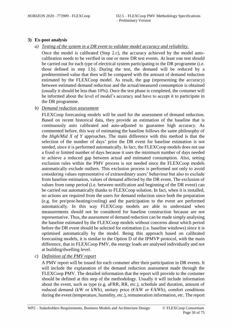
HORIZON 2020 –773909 - FLEXCoop D2.5 – FLEXCoop PMV Methodology Specifications
– Preliminary Version
WP2 – Stakeholders Requirements, Business Models and Architecture Design FLEXCoop Consortium
Page 50 of 75
3) Ex-post analysis
a) Testing of the system in a DR event to validate model accuracy and reliability.
Once the model is calibrated (Step 2.c), the accuracy achieved by the model auto-
calibration needs to be verified in one or more DR test events. At least one test should
be carried out for each type of electrical system participating to the DR programme (i.e.
those defined in step 1.b). During the test, the demand will be reduced by a
predetermined value that then will be compared with the amount of demand reduction
estimated by the FLEXCoop model. As result, the gap (representing the accuracy)
between estimated demand reduction and the actual/measured consumption is obtained
(usually it should be less than 10%). Once the test phase is completed, the costumer will
be informed about the level of model’s accuracy and have to accept it to participate in
the DR programme.
b) Demand reduction assessment
FLEXCoop forecasting models will be used for the assessment of demand reduction.
Based on recent historical data, they provide an estimation of the baseline that is
continuously auto calibrated and auto-adjusted to guarantee high accuracy. As
commented before, this way of estimating the baseline follows the same philosophy of
the High/Mid X of Y approaches. The main difference with this method is that the
selection of the number of days’ prior the DR event for baseline estimation is not
needed, since it is performed automatically. In fact, the FLEXCoop models does not use
a fixed or limited number of days because it uses the minimum number of days needed
to achieve a reduced gap between actual and estimated consumption. Also, setting
exclusion rules within the PMV process is not needed since the FLEXCoop models
automatically exclude outliers. This exclusion process is performed not only to avoid
considering values representative of extraordinary users’ behaviour but also to exclude
from baseline estimation, values of demand affected by the DR event. The exclusion of
values from ramp period (i.e. between notification and beginning of the DR event) can
be carried out automatically thanks to FLEXCoop solution. In fact, when it is installed,
no actions are required from the users for demand reduction since both the preparation
(e.g. for pre/post-heating/cooling) and the participation to the event are performed
automatically. In this way FLEXCoop models are able to understand when
measurements should not be considered for baseline construction because are not
representative. Thus, the assessment of demand reduction can be made simply analysing
the baseline estimated by the FLEXCoop models without concerns about which period
before the DR event should be selected for estimation (i.e. baseline windows) since it is
optimised automatically by the model. Being this approach based on calibrated
forecasting models, it is similar to the Option D of the IPMVP protocol, with the main
difference, that in FLEXCoop PMV, the energy loads are analysed individually and not
at building/dwelling level.
c) Definition of the PMV report
A PMV report will be issued for each costumer after their participation in DR events. It
will include the explanation of the demand reduction assessment made through the
FLEXCoop PMV. The detailed information that the report will provide to the costumer
should be defined at this step of the methodology. Usually it will include information
about the event, such as type (e.g. aFRR, RR, etc.), schedule and duration, amount of
reduced demand (kW or kWh), unitary price (€/kW or €/kWh), comfort conditions
during the event (temperature, humidity, etc.), remuneration information, etc. The report

HORIZON 2020 –773909 - FLEXCoop D2.5 – FLEXCoop PMV Methodology Specifications
– Preliminary Version
WP2 – Stakeholders Requirements, Business Models and Architecture Design FLEXCoop Consortium
Page 51 of 75
will be issued to the costumer with a periodicity according to its preferences. For
instance, it could be at the end of each DR event or on a weekly/monthly/yearly basis.
In most cases, sending remuneration information with high frequency should guarantee
a higher transparency to the programme.
The steps of the FLEXCoop PMV have been designed, not only following IPMVP and FEMP
approaches, but also considering the recommendations of NAESB [1]. According to that, it is
therefore essential that a well-defined methodology matches with the characteristics of
customers, markets and programmes and that is fair, simple and accurate to avoid lack of
transparency that is a huge barrier against the development of DR adoption. Where possible,
the methodology should be standardised and replicable, taking into account multiple standard
baselines for each type of DR activations on different consumption sites. How FLEXCoop
PMV accomplishes with these recommendations is explained at following.
Fair. FLEXCoop forecasting models will be defined and tested during the project to achieve a
standard algorithm for the baseline construction that can be applied to different types of users
and dwellings as well as in different climate conditions. These models will be part of the
FLEXCoop PMV and will provide the aggregators with a standard method to assess demand
reduction in the same way for all its customers. Furthermore, since algorithms are also
conceived for demand flexibility forecasting, estimations about potential demand reduction can
be provided to the users before the event and then compared with post assessment demand
reduction.
Accurate. FLEXCoop human centric approach foresees the measurement of the most
significant user behaviour variables that can affect the dwelling energy demand (such as
occupancy and human behaviour). In previous European project’s approaches (such as
eeMeasure) these variables were considered as immeasurable since they are dynamic and not
static, such as orientation, floor surface, envelope thermal transmittance, etc. Thanks to the
collection of this information, baselining in FLEXCoop can be provided in a more robust and
precise manner since baselining models can be continuously calibrated (continuing to improve
their accuracy while being fed with new building data), providing accurate results in short
periods. The validation of these models and going beyond typical statistical regression models
is in the core of FLEXCoop challenges. Using these types of algorithm for baseline construction
can be considered as a similar approach to High X of Y method, that has been examined in
Section 3.2.1 and is identified by the EnerNOC “Demand Response Baseline” White Paper [33]
and the KEMA “PJM Empirical Analysis of Demand Response Baseline Methods” [32] as the
best for baseline construction in most cases. In the literature, the main issue concerning this
method is the definition of the number of days needed for baseline definition. With FLEXCoop
models, this barrier is addressed, since the number of days is variable and depends on how
much time is needed to calibrate the models. Another added value of FLEXCoop models is that
they are dynamic, since learn constantly from previous data and on this basis adapt the baseline.
This aspect, together with the fact that the participation to DR event is automatized through the
FLEXCoop solution, minimizes the risk for baseline manipulation. In addition, in comparison
with previous methodologies both accuracy and precision will be higher because system loads
are measured independently (as isolated loads). This will avoid noise and errors coming from a
whole building/home measurement as well as the cross effects from other loads that are not
used for DR purposes and that can distort the assessment. This way of measurement will make
available a high number of data sample that will be useful to reduce the approximation error
and produce more accurate estimations.

HORIZON 2020 –773909 - FLEXCoop D2.5 – FLEXCoop PMV Methodology Specifications
– Preliminary Version
WP2 – Stakeholders Requirements, Business Models and Architecture Design FLEXCoop Consortium
Page 52 of 75
Simple. Measuring loads as individuals provides customers with more detailed information on
their participation in DR events. Thus, both the demand reduction assessment and the associated
remuneration can be done load by load, being for users more easy to understand. On the other
hand, since FLEXCoop model uses complex algorithms based on regression, it can result more
difficult to understand, decreasing for this reason the comprehensibility of the methodology for
the users. Nevertheless, the fact that the same algorithm is used for all customers and is
previously validated in FLEXCoop pilots will reduce this drawback. Moreover, from the side
of aggregators, the application of FLEXCoop PMV will be easier than others DR M&V
methodologies. In fact, since the analysis of historical data prior the event will automatically
be done by FLEXCoop models they do not have to perform it after each DR event. Furthermore,
being the FLEXCoop baselining method auto adaptive to recent historical data and since it
considers the actual values of all significant variables used for load estimation, a post
adjustment of baseline will not be required.
Replicable/Flexible. In the FLEXCoop framework different forecasting algorithms are created
in order to forecast and estimate all the uses that could be affected by DR event. These specific
algorithms will easily be applied to all the users and dwelling typologies as well as different
climate conditions. Despite they are designed for standard use cases, since they are fed with
real-time monitoring data they are calibrated in each specific dwelling ensuring accurate
predictions for each specific case. In addition, since they auto-adapt themselves to extraordinary
circumstances such as excessively high load on event days and to possible changes in
occupancy, user-behaviours, environmental conditions, etc. their flexibility in different
conditions and for different types of users is guaranteed. Thanks to these algorithms, the
FLEXCoop model provides a high flexibility, allowing the application of the FLEXCoop PMV
in different contexts.
6. KPIS DEFINITION
This section provides adequate Key Performance Indicators (KPIs) needed to assess the results
of demand flexibility achieved by FLEXCoop, that is, the optimization of the energy
performance at pilot sites, by, for example, measuring the efficiency of load shifting
mechanisms under user’s comfort conditions. The deliverable defines various interrelated
evaluation categories, each of which consists of independent KPIs. KPIs are deviated from
FLEXCoop Use Cases (UCs), which have also been correlated to Business Scenarios (BSs). A
brief summary of UCs with collaborated BSs are presented in this deliverable. For more
information, the reader is referred to FLEXCoop D2.1 and D2.4. For each KPI, the calculation
method with the formulas used and monitoring needed to determine the performance of the
parameters along with linked UC(s) and BS(s) is presented. After the initial design and
implementation of pilots, PMV must be re-evaluated and KPIs must be revised with
modifications suggested based on experience that will be acquired after system deployment in
pilot sites. As a result, we, first, overview BSs and UCs followed by a briefly presentation of
the KPIs based on different categories. Appendix A details KPIs thoroughly.
6.1. Overview of Business Scenarios
BSs have been made in such a way that are acceptable for cooperatives as business
models to extend their business portfolio with explicit DR solutions. FLEXCoop has defined
the following six BSs (see D2.1 and D2.4 for more details) as follows:

HORIZON 2020 –773909 - FLEXCoop D2.5 – FLEXCoop PMV Methodology Specifications
– Preliminary Version
WP2 – Stakeholders Requirements, Business Models and Architecture Design FLEXCoop Consortium
Page 53 of 75
BS1: Energy efficiency, comfort and self-generation monitoring
o This scenario concerns the providing of an increased comfort and control over
the equipment and (automation of) devices.
BS2-A: Self-consumption optimisation of Distributed Energy Resources (DER)
o This scenario enables cooperative (retailer) to employ consumers’ flexibility to
match better with the production patterns of generation assets and optimisation
of self-generation assets.
BS2-B: Consumption optimisation of energy bought on wholesale market
o This scenario utilizes consumers’ flexibility to better match the anticipated
prices on wholesale market – encouraging consumption at low hours and
avoiding consumption at peak hours by offering cheaper electricity.
BS3: Participation into balancing and ancillary services
o This scenario, by using the flexibility, aims at providing grid system actors,
e.g., TSO and DSO, with ancillary services, such as balancing or congestion
management, based on contractual agreement in place.
BS4: Microgrid-as-a-Service
o This scenario realizes the real-time management of decentralized generation
and consumption (smart appliances) by offering the possibility of not relying
on the grid anymore (i.e. to become a microgrid, independent form the power
market).
BS5: Neutral platform for aggregator- prosumer matching
o This scenario, by using FLEXCoop solution as a platform service (like Uber or
Airbnb, aims to facilitate contracting between prosumers and aggregators at a
wide scale.
6.2. Overview of Use Cases
From the defined set of BSs, a list of UCs is proposed for cooperatives as
domestic demand flexibility aggregators. Table 2 lists the FLEXCoop functional use cases list
along with correlated BSs. For more information, please refer to D2.1.
Table 2: FLEXCoop functional use cases list along with correlated BSs
UC UC description Correlated BS
1 Extraction of personalized (dis)comfort profiles towards the
establishment of a user-centred management framework
BS1, BS3, BS4
2 Extraction of context-aware demand flexibility profiles BS2(A&B),
BS3, BS4
3 Establishment of a data analytics framework for the optimal
portfolio management
BS2(A&B),
BS3, BS4
4 Establishment of a real time fully automated DR triggering
framework
BS2(A&B),
BS3, BS4
5 Real time monitoring of DR strategies implementation and re-
configuration of dynamic VPPs
BS2(A&B),
BS3, BS4
6 DR settlement and prosumer remuneration for DR participation BS3 BS4
7 Establishment of DER Registry to ensure the openness of energy
market to the final customers
(BS2), BS3,
BS4

HORIZON 2020 –773909 - FLEXCoop D2.5 – FLEXCoop PMV Methodology Specifications
– Preliminary Version
WP2 – Stakeholders Requirements, Business Models and Architecture Design FLEXCoop Consortium
Page 54 of 75
8 Establishment of Flexibility Pooling and Sharing Marketplace to
promote end user’s empowerment in energy market
BS3, BS4, BS5
9 Promotion of self-consumption concept for maximizing
consumption from local generation units
BS2, BS4
9 bis Promotion of system efficiency concept for optimising energy
purchase on wholesale market based on price or CO2 content
BS2
10 Cooperative-operated microgrids towards the establishment of
independent entities in distribution grid
(BS2) BS4
11 Prosumers awareness and knowledge about their consumption
patterns- Engagement to the overall framework
BS1,
BS2(A&B),
BS3, BS4
11 bis Prosumers on delivered services and resulting remuneration –
Transparency of the overall framework
BS2(A&B),
BS3, BS4
12 Prosumer level self-consumption to maximize energy
consumption when high RES generation
BS2(A&B),
BS3, BS4
6.3. Categorized KPIs
6.3.1. Category of Energy
Table 3 provides Energy KPIs for quantifying the (renewable) electricity
consumption/production as well as energy saving.
Table 3: KPIs proposed for evaluation of the category of Energy
KPI ID Name Description
ENE 1 Self-consumption
ratio
Measuring the efficiency of load shifting mechanisms and
energy storage by quantifying the amount of electricity
produced and consumed locally relative to the total local
production available from on-site generation units
ENE 2 Energy saving Quantifying the difference between measured and reference
consumption data within a predefined period
ENE 3 (Buildings) Final
consumption
Quantifying the total amount of energy consumed in a building
(or in a part of it) within a predefined period
ENE 4 Total renewable
energy
consumption
Quantifying the total amount of renewable energy (electricity)
consumed in a building (or in a part of it) within a predefined
period
6.3.2. Category of DR and Flexibility
Table 4 provides DR and Flexibility KPIs for tracking customer’s participation in DR programs in
the FLEXCoop pilot sites, quantifying the aggregated flexibility, and measuring the peak load reduction.
Table 4: KPIs proposed for evaluation of the category of DR and Flexibility
KPI ID Name Description
DRF 1 DR participation
adoption
Tracking the increase of customers participation in DR
programs in the FLEXCoop pilot sites
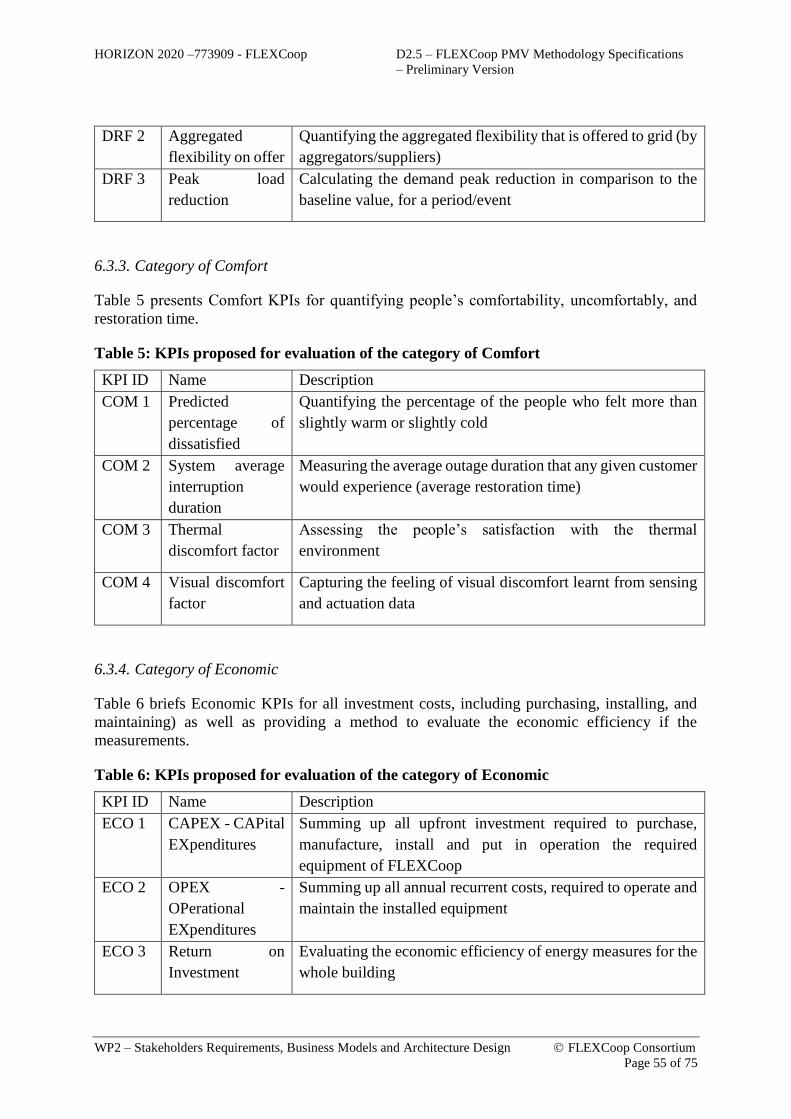
HORIZON 2020 –773909 - FLEXCoop D2.5 – FLEXCoop PMV Methodology Specifications
– Preliminary Version
WP2 – Stakeholders Requirements, Business Models and Architecture Design FLEXCoop Consortium
Page 55 of 75
DRF 2 Aggregated
flexibility on offer
Quantifying the aggregated flexibility that is offered to grid (by
aggregators/suppliers)
DRF 3 Peak load
reduction
Calculating the demand peak reduction in comparison to the
baseline value, for a period/event
6.3.3. Category of Comfort
Table 5 presents Comfort KPIs for quantifying people’s comfortability, uncomfortably, and
restoration time.
Table 5: KPIs proposed for evaluation of the category of Comfort
KPI ID Name Description
COM 1 Predicted
percentage of
dissatisfied
Quantifying the percentage of the people who felt more than
slightly warm or slightly cold
COM 2 System average
interruption
duration
Measuring the average outage duration that any given customer
would experience (average restoration time)
COM 3 Thermal
discomfort factor
Assessing the people’s satisfaction with the thermal
environment
COM 4 Visual discomfort
factor
Capturing the feeling of visual discomfort learnt from sensing
and actuation data
6.3.4. Category of Economic
Table 6 briefs Economic KPIs for all investment costs, including purchasing, installing, and
maintaining) as well as providing a method to evaluate the economic efficiency if the
measurements.
Table 6: KPIs proposed for evaluation of the category of Economic
KPI ID Name Description
ECO 1 CAPEX - CAPital
EXpenditures
Summing up all upfront investment required to purchase,
manufacture, install and put in operation the required
equipment of FLEXCoop
ECO 2 OPEX -
OPerational
EXpenditures
Summing up all annual recurrent costs, required to operate and
maintain the installed equipment
ECO 3 Return on
Investment
Evaluating the economic efficiency of energy measures for the
whole building

HORIZON 2020 –773909 - FLEXCoop D2.5 – FLEXCoop PMV Methodology Specifications
– Preliminary Version
WP2 – Stakeholders Requirements, Business Models and Architecture Design FLEXCoop Consortium
Page 56 of 75
6.3.5. Category of System Reliability
Table 7 introduces System Reliability KPIs for measuring the load forecasting accuracy and
validating the data reliability.
Table 7: KPIs proposed for evaluation of the category of System Reliability
KPI ID Name Description
SYR 1 Load forecasting
accuracy
Measuring the mean absolute percentage error between the
forecasted and the current load
SYR 2 Data validation
ratio
Calculating the percentage of validated data according to all
the data received in a time
6.3.6. Category of Security and Privacy
X lists Security and Privacy KPIs for assessing the level of data privacy collected in the
FLEXCoop project that meet GDPR requirements.
KPI ID Name Description
SEP 1 GDPR risk Assessing the level of data privacy collected in the FLEXCoop
project to get how many of regulation standards are met
Correlation between BSs, UCs, and KPIs Table 8 consolidates the correlations/dependencies
among various BSs, UCs, and KPIs defined.
Table 8: Consolidated correlations/dependencies among defined BSs, UCs, and KPIs
Category KPI ID BS UC
Energy
ENE 1
BS1,
BS2(A&B),
BS3, BS4
UC1, UC2, UC4, UC6, UC9, UC9 bis,
UC12
ENE 2 UC1, UC2, UC4, UC6, UC9, UC9 bis,
UC11, UC11 bis, UC12
ENE 3 UC1, UC2, UC4, UC6, UC9, UC9 bis,
UC11, UC11 bis, UC12
ENE 4 UC1, UC2, UC4, UC6, UC9, UC9 bis,
UC11, UC11 bis, UC12
DR and Flexibility
DRF 1 UC3, UC6, UC8
DRF 2 UC3, UC6, UC8
DRF 3 UC1, UC2, UC6, UC9, UC9 bis
Comfort
COM 1 UC1, UC2, UC6, UC11, UC12
COM 2 UC1, UC2, UC4, UC6, UC11, UC12
COM 3 UC1, UC2, UC9, UC9 bis, UC11
COM 4 UC1, UC2, UC9, UC9 bis, UC11
Economic
ECO 1 UC3, UC4, UC5, UC7, UC12
ECO 2 UC3, UC4, UC5, UC7, UC12
ECO 3 UC3, UC4, UC5, UC7, UC12
System Reliability SYR 1 UC1, UC2, UC11, UC12

HORIZON 2020 –773909 - FLEXCoop D2.5 – FLEXCoop PMV Methodology Specifications
– Preliminary Version
WP2 – Stakeholders Requirements, Business Models and Architecture Design FLEXCoop Consortium
Page 57 of 75
SYR 2 UC1, UC2, UC5, UC7, UC11, UC11 bis,
UC12
Security and Privacy SEP 1 UC1 - UC12

HORIZON 2020 –773909 - FLEXCoop D2.5 – FLEXCoop PMV Methodology Specifications
– Preliminary Version
WP2 – Stakeholders Requirements, Business Models and Architecture Design FLEXCoop Consortium
Page 58 of 75
7. CONCLUSION
The main conclusions of the first part of FLEXCoop Task 2.4 on “Definition of Monitoring and
Verification Methodology for DR settlement and remuneration and Key Performance
Indicators” are summarised in the list of steps that compose the FLEXCoop PMV:
1) Ex-ante analysis
a) Definition of DR events and criteria for remuneration.
b) Definition of DR systems and minimum comfort conditions
c) Identification of static and dynamic variables that affect the demand and need to be
measured.
2) Implementation
a) Analysis of existing monitoring system and specification of metering points’ and
sensors’ characteristics.
b) Analysis of the technical and economic reliability of individual loads measurements.
c) Conduct post-installation verification activities for algorithm calibration.
3) Ex-post analysis
a) Testing of the system in a DR event to validate model accuracy and reliability.
b) Demand reduction assessment
c) Definition of the PMV report
The methodology is the main outcome of the work carried on in this task. Other relevant
findings have been achieved through the analysis of previous EU projects and of existent
literature in the fields of M&V applied to energy efficiency and DR. Thanks to this initial work,
how the FLEXCoop PMV allows going beyond normal practices in M&V in DR has been
detected. Main barriers addressed by the FLEXCoop PMV are:
- FLEXCoop models used for baselining calculation treat occupancy and human actions
as dependent variables and for this reason are measurable (and not immeasurable as in
the eeMeasure methodology) and allow higher accuracy.
- In FLEXCoop PMV, data required for baseline calibration are needed only for the last
days/weeks and not for a completely operational cycle.
- The selection of historical data for baselining calibration and adjustment is made
automatically by the FLEXCoop models that select the minimum number of days
needed to achieve an acceptable baseline accuracy. In this way, the issue related to
which period considers to select representative days is solved, as well as the necessity
of performing adjustment to the baseline (and select an adjustment window) after the
DR event is not needed since it is carried out automatically.
- Baseline methods that use recent historical data between notification and beginning of
the DR event for baselining construction are opened to the risk of manipulation by users,
Since FLEXCoop solution provides an automated control of the systems used to give
response when a DR event is called, manipulation is limited. Also in the case that user
tries to increase the loads more than the necessary to get an over-remuneration,
FLEXCoop models will be able to detect it thanks to the user behaviour’s models that
will detect an unusual action and will exclude it for baseline calibration.

HORIZON 2020 –773909 - FLEXCoop D2.5 – FLEXCoop PMV Methodology Specifications
– Preliminary Version
WP2 – Stakeholders Requirements, Business Models and Architecture Design FLEXCoop Consortium
Page 59 of 75
- As consequence of a continuous auto-calibration of the forecasting models a very high
accuracy will be achieved. This would allow the application of Option D that usually is
very complicated due to the high accuracy required by the IPMVP. Nevertheless, this
option does not represent as whole the FLEXCoop PMV since measurements for model
calibration are made at load and not at building level, being in this case, closer to Option
B.
The literature research has been also useful to verify that the approach proposed by FLEXCoop
complies with main recommendations stated in the last years on the basis of previous practical
experiences in PMV methods. In this Task 2.4, also a list of KPIs to assess the results of demand
flexibility achieved by FLEXCoop has been identified and organised in six evaluation
categories during this task. KPIs are derived from FLEXCoop Use Cases (UCs), which have
also been translated to Business Scenarios (BSs). Further validation of the FLEXCoop PMV
and of KPIs’ lists will be carried out in the second phase of this Task 2.4, when the method will
be implemented in FLEXCoop friendly user’s pilots.

HORIZON 2020 –773909 - FLEXCoop D2.5 – FLEXCoop PMV Methodology Specifications
– Preliminary Version
WP2 – Stakeholders Requirements, Business Models and Architecture Design FLEXCoop Consortium
Page 60 of 75
8. LITERATURE
[1] D. Holmberg, D. Hardin y E. Koch, Towards Demand Response Measurement and Verification
Standards, 2013.
[2] Australasian Energy Performance Contracting Association, A best practice guide to
measurement and verification of energy savings. A companion document to ‘A best practice
guide to energy performance contracts’, 2004.
[3] [Online]. Available: https://evo-world.org/en/about-en/history-mainmenu-en.
[4] Efficiency Valuation Organization (EVO), International Performance Measurement &
Verification Protocol. Concepts and Options for Determining Energy and Water Savings,
Volume I, 2010.
[5] Efficiency Valuation Organization (EVO),, International performance measurement &
verification protocol. Concepts and practices for improved indoor environmental quality.
Volume II., 2002.
[6] United States Department of Energy (DOE), M&V guidelines: measurement and verification
for performance-based contracts version 4.0, 2015.
[7] American Society of Heating, Refrigerating and Air-Conditioning Engineers (ASHRAE),
Guideline 14-2002 – Measurement of energy and demand savings, 2002.
[8] European Committee for Standardization (CEN), EN 16212:2012 ‘Energy efficiency and
savings calculation, top-down and bottom-up methods’, 2012.
[9] The European Parliament and the Council of the European Union, Directive 2006/32/EC of the
European Parliament and of the Council on energy end-use efficiency and energy services
and repealing council directive 93/76/EEC, 2006.
[10] International Organization for Standardization (ISO), ISO 50015:2014 Energy management
systems – Measurement and verification of energy performance of organizations – General
principles and guidance, 2014.
[11] International Organization for Standardization (ISO), ISO 50001:2011 Energy management
systems – Requirements with guidance for use, 2011.
[12] International Organization for Standardization (ISO), ISO 17741:2016 General technical rules
for measurement, calculation and verification of energy savings of projects, 2016.
[13] European Comission, [En línea]. Available:
http://iet.jrc.ec.europa.eu/energyefficiency/european-energy-service-
companies/monitoring-and-verification.
[14] Efficiency Valuation Organization, «International Performance Measurement and Verification
Protocol. Concepts and Options for Determining,» January 2012. [En línea]. Available:
http://www.eeperformance.org/uploads/8/6/5/0/8650231/ipmvp_volume_i__2012.pdf.
[15] FEMP of the US Department of Energy, «M&V Guidelines: Measurement and Verification for
Performance-Based Contracts Version 4.0, Federal Energy Management Program,»
November 2015. [En línea]. Available:
https://www.energy.gov/sites/prod/files/2016/01/f28/mv_guide_4_0.pdf.
[16] Efficiency Valuation Organization (EVO), International performance measurement &
verification protocol. Concepts and practices for improved indoor environmental quality.
Volume II., 2002.

HORIZON 2020 –773909 - FLEXCoop D2.5 – FLEXCoop PMV Methodology Specifications
– Preliminary Version
WP2 – Stakeholders Requirements, Business Models and Architecture Design FLEXCoop Consortium
Page 61 of 75
[17] Efficiency Valuation Organization (EVO), International performance measurement &
verification protocol. Concepts and practices for determining energy savings in new
construction. Volume III Part I., 2006.
[18] Efficiency Valuation Organization (EVO), International performance measurement &
verification protocol. Concepts and practices for determining energy savings in renewable
energy technologies applications. Volume III Part II, 2003.
[19] [En línea]. Available: https://evo-world.org/en/products-services-mainmenu-
en/protocols/ipmvp .
[20] U.S. Department of Energy, «Federal Energy Management Program,» Feb 2016. [En línea].
Available:
https://www.energy.gov/sites/prod/files/2016/02/f29/fed_energy_mgmt_program.pdf.
[21] AEIC Load Research Committee, «Demand Response Measurement & Verification,» 2009.
[En línea]. Available: https://www.smartgrid.gov/files/demand_response.pdf.
[22] European Union, «EEmeasure,» [En línea]. Available: http://eemeasure.smartspaces.eu/.
[23] European Commission, «The ICT PSP methodology for energy saving measurement - a
common deliverable from projects of ICT for sustainable growth in the residential sector,»
April 2012. [En línea]. Available:
http://eemeasure.smartspaces.eu/static/files/eemeasure_residential_methodology.pdf.
[24] G. Woodall, «SMART 2011 / 0072: Methodology for energy-efficiency measurements
applicable to ICT in buildings (eeMeasure): D1.5 Non-residential methodology,» 2011.
[En línea]. Available:
http://eemeasure.smartspaces.eu/static/files/eemeasure_non_residential_methodology.pdf.
[25] European Commission, «Moeebius project,» [En línea]. Available: http://www.moeebius.eu/.
[26] Moeebius Project, «Energy performance assessment methodology,» 2016. [En línea].
Available: http://www.moeebius.eu/333-report-moeebius-energy-performance-
assessment-methodology.
[27] Federal Energy Management Program, US Department of Energy, «FEMP, M&V Guidelines:
Measurement and Verification for Performance-Based Contracts Version 4.0,» November
2015.
[28] OrbEEt project, [En línea]. Available: http://orbeet.eu/.
[29] OrbEEt, «D1.2 Energy Measurements Methodology,» 2016.
[30] HOLISDER, «HOLISDER project,» [En línea]. Available: http://holisder.eu/.
[31] North American Standard Energy Standards Board (NAESB), WEQ Annual Plan Item 4(a) and
4(b) Final Action: Review and develop business practice standards to support DR and
DSM-EE programs., 2010.
[32] KEMA, PJM Empirical Analysis of Demand Response Baseline Methods., 2011.
[33] Enernoc, The Demand Response Baseline, 2009.
[34] Association of Edison Illuminating Companies (AEIC), Demand Response Measurements &
Verification, 2009.
[35] Efficiency Valuation Organization (EVO), Uncertainty Assessment for IPMVP - Release of a
New IPMVP Application Guide, 2018.
[36] California Energy Commission , Protocol Development for Demand Response Calculation.
Draft and Findings., 2002.

HORIZON 2020 –773909 - FLEXCoop D2.5 – FLEXCoop PMV Methodology Specifications
– Preliminary Version
WP2 – Stakeholders Requirements, Business Models and Architecture Design FLEXCoop Consortium
Page 62 of 75
[37] ERCOT Demand Side Working Group (Freeman, Sullivan & Co.), Empirical Data on
Settlement of Weather Sensitive Loads., 2012.
[38] Southern California Edison , Southern California Edison Company Demand Response
Appendices to SCE-1, Volumes 1-4, 2011.
[39] Diao, Lu, Elizondo, Mayhorn, Zhang y Samaan, Electric Water Heater Modeling and Control
Strategies for Demand Response, 2012.
[40] A. Sepulveda, L. Paull, W. Morsi, H. Li, C. Diduch y L. Chang, A Novel Demand Side
Management Program using Water Heaters and Particle Swarm Optimization, 2010.
[41] European Commission, «REGULATION (EU) 2016/679 on the protection of natural persons
with regard to the processing of personal data and on the free movement of such data, and
repealing Directive 95/46/EC (General Data Protection Regulation),» 2016. [En línea].
Available: https://eur-lex.europa.eu/legal-
content/EN/TXT/HTML/?uri=CELEX:32016R0679&from=EN.
[42] M. L. Goldberg y G. K. Agnew, «Measurement and Verification for Demand Response,»
U.S.A, 2013.
[43] D. Holmberg, D. Hardin y E. Koch, «Towards Demand Response Measurement and
Verification Standards,» 2013.

HORIZON 2020 –773909 - FLEXCoop D2.5 – FLEXCoop PMV Methodology Specifications
– Preliminary Version
WP2 – Stakeholders Requirements, Business Models and Architecture Design FLEXCoop Consortium
Page 63 of 75
APPENDIX A
The following tables present the detail of categorized KPIs briefed in Section 6.
Energy KPIs
KPI ID ENE 1
Name Self-consumption ratio
Category Energy
Related Use Cases UC1, UC2, UC4, UC6, UC9, UC9 bis, UC12
Description
Self-consumption ratio is a metric used for quantifying the amount of
electricity produced and consumed locally relative to the total production
that is locally available from on-site generation units. It is calculated as the
ratio of self-consumption divided by the self-generated energy.
Formula
𝑆𝐶𝑅 =∑ min(𝑃𝑡 , 𝐷𝑡)𝑡∈𝑇
∑ 𝑃𝑡𝑡∈𝑇100
𝑆𝐶𝑅: self-consumption ratio
𝑇: evaluation period
𝑡: metering period (e.g. 15 minutes)
𝑃𝑡: energy produced by on-site generation/energy drawn from on-site
storage unit during metering period 𝑡 (by the whole portfolio or on the
customer permises) (kWh)
𝐷𝑡: energy demand during metering period 𝑡 (by the whole portfolio or on
the customer premises) (kWh)
Unit of
measurement %
GENERAL COMMENTS
The SCR is usually calculated over a certain time period (e.g. a year).
This KPI aims to measure the efficiency of load shifting mechanisms and energy storage towards
increasing the ratio of energy produced by members of the portfolio that is self-consumed within
the portfolio. However, this KPI could also be used for individual evaluation of self-consumption
per customer.
Higher value of the ratio signifies that the best use of the locally generated energy is made, since
it is consumed locally.

HORIZON 2020 –773909 - FLEXCoop D2.5 – FLEXCoop PMV Methodology Specifications
– Preliminary Version
WP2 – Stakeholders Requirements, Business Models and Architecture Design FLEXCoop Consortium
Page 64 of 75
KPI ID ENE 2
Name Energy savings (electricity)
Category Energy
Related Use Cases UC1, UC2, UC4, UC6, UC9, UC9 bis, UC11, UC11 bis, UC12
Description
This indicator is usually used for project evaluation (where suppliers are
involved), and for consumer behaviour change (for consumers). It will
measure the difference between measured and reference consumption data,
evaluated within a predefined period of time.
Formula
𝐸𝑆 =∑ ∑ |𝐶𝐵𝐿𝑛ℎ
𝑛− 𝐿ℎ|
ℎ∈𝐻
𝐶𝐵𝐿𝑛ℎ : baseline load of user 𝑛 during time interval ℎ of the period under
study (kWh/h)
𝐿ℎ = ∑ 𝑙𝑛ℎ
𝑛∈𝑁 : the total power of the load across all users 𝑛 ∈ 𝑁 during
each time interval ℎ of the period under study (kWh/h)
𝑙𝑛ℎ: the load of user 𝑛 during time interval ℎ of the period under study
(kWh/h)
𝐻: the set of time intervals of the period under study (ℎ ∈ 𝐻)
𝑁: the set of customers under study (𝑛 ∈ 𝑁)
Unit of
measurement kWh

HORIZON 2020 –773909 - FLEXCoop D2.5 – FLEXCoop PMV Methodology Specifications
– Preliminary Version
WP2 – Stakeholders Requirements, Business Models and Architecture Design FLEXCoop Consortium
Page 65 of 75
GENERAL COMMENTS
KPI ID ENE 3
Name Buildings final energy consumption/demand
Category Energy
Related Use Cases UC1, UC2, UC4, UC6, UC9, UC9 bis, UC11, UC11 bis, UC12
Description This KPI aims to show the total amount of energy consumed in a building
(or in a part of it) in a time period.
Formula
BFEC =∑ 𝐵𝐹𝐶ℎ∈𝐻𝑛
𝑛∈𝑁 ; 𝑆𝐵𝐹𝐸𝐶 =𝐵𝐹𝐸𝐶
𝑆
𝑁: set of customers under study (𝑛 ∈ 𝑁)
𝐻: the set of time intervals of the period under study (ℎ ∈ 𝐻)
BFC: Building final consumption (kWh)
SBFEC: Building final energy consumption per surface unit (kWh/m2)
S: Surface (m2)
Unit of
measurement kWh ; kWh/m2
GENERAL COMMENTS
KPI ID ENE 4
Name Renewable total energy consumption
Category Energy
Related Use Cases UC1, UC2, UC4, UC6, UC9, UC9 bis, UC11, UC11 bis, UC12
Description
This KPI aims to show the total amount of renewable energy (electricity)
consumed in a building (or in a part of it) in a time period. It will also show
its proportion concerning the total energy consumed.
Formula RE =∑ 𝑅𝐶ℎ∈𝐻𝑛
𝑛∈𝑁 ; %𝑁𝑅𝐸 =𝑅𝐸
𝐵𝐹𝐸𝐶× 100

HORIZON 2020 –773909 - FLEXCoop D2.5 – FLEXCoop PMV Methodology Specifications
– Preliminary Version
WP2 – Stakeholders Requirements, Business Models and Architecture Design FLEXCoop Consortium
Page 66 of 75
𝑁: set of customers under study (𝑛 ∈ 𝑁)
𝐻: the set of time intervals of the period under study (ℎ ∈ 𝐻)
RC: Renewable energy consumption (kWh)
%NRC: Non-Renewable energy consumption
BFEC: Building Final Energy Consumption (kWh)
Unit of
measurement kWh ; %
GENERAL COMMENTS
DR and Flexibility KPIs
KPI ID DRF 1
Name DR participation analysis
Category DR & Flexibility
Related Use Cases UC3, UC6, UC8
Description
This KPI aims to track the increase of customers participation in DR
programs in the FLEXCoop pilot sites, hence to quantify the improvement
in adopting DR mechanisms among these final customers, due to
implementation of the FLEXCoop system.
Formula
𝐷𝑅𝑃𝑃 =𝑁𝐶𝑎𝑓𝑡𝑒𝑟
−𝑁𝐶𝑏𝑒𝑓𝑜𝑟𝑒
𝑁𝐶𝑏𝑒𝑓𝑜𝑟𝑒
100
𝐷𝑅𝑃𝑃: DR participation penetration
𝑁𝐶𝑏𝑒𝑓𝑜𝑟𝑒
: Numbers of customers active in DR programs before system
deployment and pilot rollout
𝑁𝐶𝑎𝑓𝑡𝑒𝑟
: Numbers of customers active in DR programs after system
deployment and pilot rollout
Unit of
measurement %
GENERAL COMMENTS

HORIZON 2020 –773909 - FLEXCoop D2.5 – FLEXCoop PMV Methodology Specifications
– Preliminary Version
WP2 – Stakeholders Requirements, Business Models and Architecture Design FLEXCoop Consortium
Page 67 of 75
KPI ID DRF 2
Name Flexibility on offer
Category DR & Flexibility
Related Use Cases UC3, UC6, UC8
Description This KPI aims to quantify the aggregated flexibility that is offered to grid
operators by aggregators/suppliers.
Formula
The maximum demand flexibility that is on offer by an aggregator and/or
supplier can be quantified as follows:
maxℎ∈𝐻
∑ 𝐷𝐹ℎ𝑛
𝑛∈𝑁
𝐷𝐹ℎ𝑛: demand flexibility profile of individual consumer 𝑛 during interval ℎ
(kWh)
𝑁: set of customers under study (𝑛 ∈ 𝑁)
𝐻: the set of time intervals of the period under study (ℎ ∈ 𝐻)
Unit of
measurement kWh
GENERAL COMMENTS
KPI ID DRF 3
Name Peak load reduction
Category DR & Flexibility
Related Use Cases UC1, UC2, UC6, UC9, UC9 bis
Description
Peak Load Reduction captures a significant aspect of DR, in the sense that
it quantifies, for a particular period of time/event, how much demand was
reduced, in comparison to the baseline value.
Formula
𝑳𝑹 = (𝟏 −𝑳𝒂𝒄𝒕𝑷𝑳𝒃𝒍
) ∗ 𝟏𝟎𝟎
where:
PLR: Peak Load Reduction
Lact: actual Load at the moment of expected/baseline peak load during the
day of the intervention
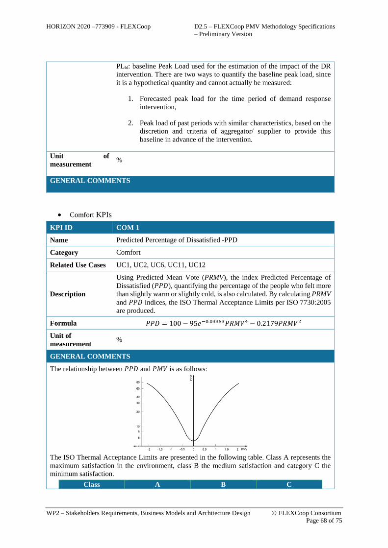
HORIZON 2020 –773909 - FLEXCoop D2.5 – FLEXCoop PMV Methodology Specifications
– Preliminary Version
WP2 – Stakeholders Requirements, Business Models and Architecture Design FLEXCoop Consortium
Page 68 of 75
PLbl: baseline Peak Load used for the estimation of the impact of the DR
intervention. There are two ways to quantify the baseline peak load, since
it is a hypothetical quantity and cannot actually be measured:
1. Forecasted peak load for the time period of demand response
intervention,
2. Peak load of past periods with similar characteristics, based on the
discretion and criteria of aggregator/ supplier to provide this
baseline in advance of the intervention.
Unit of
measurement %
GENERAL COMMENTS
Comfort KPIs
KPI ID COM 1
Name Predicted Percentage of Dissatisfied -PPD
Category Comfort
Related Use Cases UC1, UC2, UC6, UC11, UC12
Description
Using Predicted Mean Vote (PRMV), the index Predicted Percentage of
Dissatisfied (𝑃𝑃𝐷), quantifying the percentage of the people who felt more
than slightly warm or slightly cold, is also calculated. By calculating PRMV
and 𝑃𝑃𝐷 indices, the ISO Thermal Acceptance Limits per ISO 7730:2005
are produced.
Formula 𝑃𝑃𝐷 = 100 − 95𝑒−0.03353𝑃𝑅𝑀𝑉4 − 0.2179𝑃𝑅𝑀𝑉2
Unit of
measurement %
GENERAL COMMENTS
The relationship between 𝑃𝑃𝐷 and 𝑃𝑀𝑉 is as follows:
The ISO Thermal Acceptance Limits are presented in the following table. Class A represents the
maximum satisfaction in the environment, class B the medium satisfaction and category C the
minimum satisfaction.
Class A B C
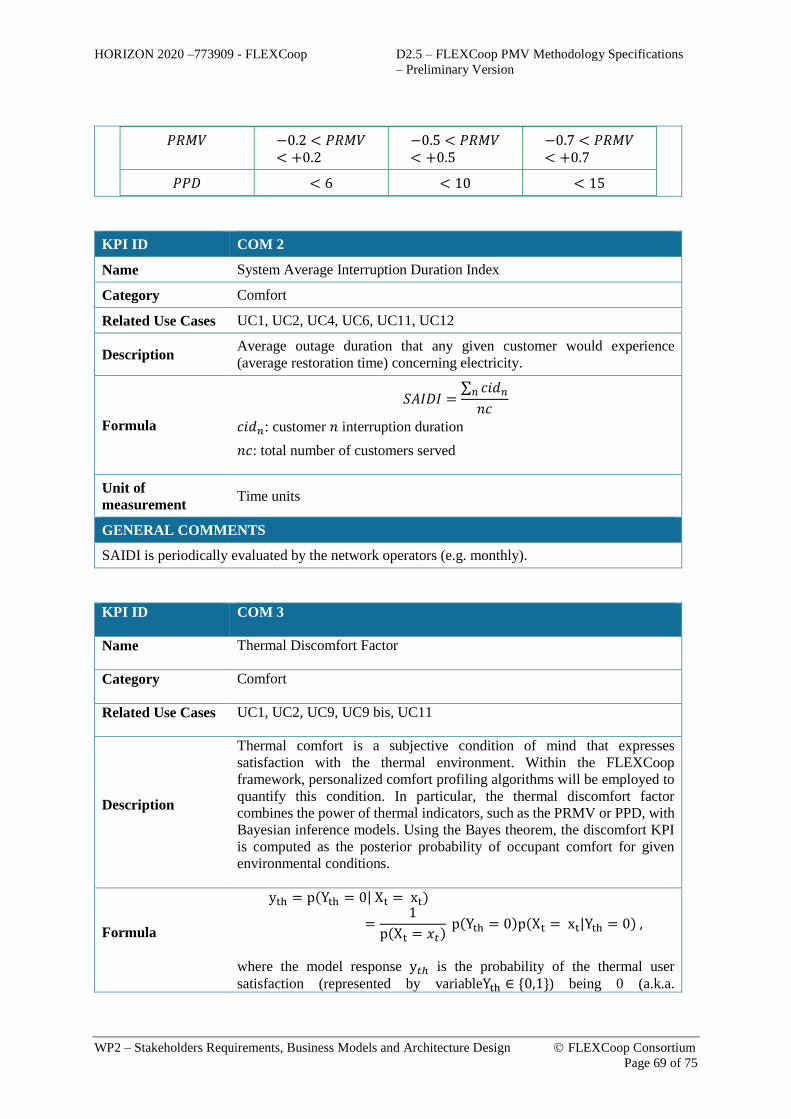
HORIZON 2020 –773909 - FLEXCoop D2.5 – FLEXCoop PMV Methodology Specifications
– Preliminary Version
WP2 – Stakeholders Requirements, Business Models and Architecture Design FLEXCoop Consortium
Page 69 of 75
𝑃𝑅𝑀𝑉 −0.2 < 𝑃𝑅𝑀𝑉< +0.2
−0.5 < 𝑃𝑅𝑀𝑉< +0.5
−0.7 < 𝑃𝑅𝑀𝑉< +0.7
𝑃𝑃𝐷 < 6 < 10 < 15
KPI ID COM 2
Name System Average Interruption Duration Index
Category Comfort
Related Use Cases UC1, UC2, UC4, UC6, UC11, UC12
Description Average outage duration that any given customer would experience
(average restoration time) concerning electricity.
Formula
𝑆𝐴𝐼𝐷𝐼 =∑ 𝑐𝑖𝑑𝑛𝑛
𝑛𝑐
𝑐𝑖𝑑𝑛: customer 𝑛 interruption duration
𝑛𝑐: total number of customers served
Unit of
measurement Time units
GENERAL COMMENTS
SAIDI is periodically evaluated by the network operators (e.g. monthly).
KPI ID COM 3
Name Thermal Discomfort Factor
Category Comfort
Related Use Cases UC1, UC2, UC9, UC9 bis, UC11
Description
Thermal comfort is a subjective condition of mind that expresses
satisfaction with the thermal environment. Within the FLEXCoop
framework, personalized comfort profiling algorithms will be employed to
quantify this condition. In particular, the thermal discomfort factor
combines the power of thermal indicators, such as the PRMV or PPD, with
Bayesian inference models. Using the Bayes theorem, the discomfort KPI
is computed as the posterior probability of occupant comfort for given
environmental conditions.
Formula
yth = p(Yth = 0|Xt = xt)
=1
p(Xt = 𝑥𝑡)p(Yth = 0)p(Xt = xt|Yth = 0),
where the model response y𝑡ℎ is the probability of the thermal user
satisfaction (represented by variableYth ∈ {0,1}) being 0 (a.k.a.

HORIZON 2020 –773909 - FLEXCoop D2.5 – FLEXCoop PMV Methodology Specifications
– Preliminary Version
WP2 – Stakeholders Requirements, Business Models and Architecture Design FLEXCoop Consortium
Page 70 of 75
dissatisfied). xt denotes the input condition variable, which can be selected
from among various options (PRMV, PPD, temperature, etc.).
Unit of
measurement Probability (0-1)
GENERAL COMMENTS
The Thermal Discomfort Factor constitutes a basis for the comfort and flexibility profiling
framework of the FLEXCoop project and will be described in detail in later deliverables. The
model requires training from monitored sensing and actuation data. The lack of control actions is
translated as user comfort, while modification of the HVAC operation is taken to be an indicator
of discomfort for the occupant.
KPI ID COM 4
Name Visual Discomfort Factor
Category Comfort
Related Use Cases UC1, UC2, UC9, UC9 bis, UC11
Description
Similar to the previous KPI, the Visual Discomfort Factor is a personalized
metric regarding the feeling of visual discomfort learnt from sensing and
actuation data. Again, this KPI is computed as the posterior probability of
occupant comfort for given luminance conditions.
Formula
y𝑣𝑖𝑠 = p(Y𝑣𝑖𝑠 = 0|X𝑣 = x𝑣)
=1
p(X𝑣 = 𝑥𝑣)p(Y𝑣𝑖𝑠 = 0)p(X𝑣 = x𝑣|Y𝑣𝑖𝑠 = 0),
where the model response y𝑣𝑖𝑠 is the probability of the user satisfaction
(represented by variable Y𝑣𝑖𝑠 ∈ {0,1}) being 0 (a.k.a. dissatisfied). x𝑣
denotes the input condition variable, which can be selected from among
visual metrics, such as luminance or illuminance.
Unit of
measurement Probability (0-1)
GENERAL COMMENTS
The Visual Discomfort Factor constitutes a basis for the comfort and flexibility profiling
framework of the FLEXCoop project and will be described in detail in later deliverables. The
model requires training from monitored sensing and actuation data. The lack of control actions is
translated as user comfort, while modification of the lighting system operation is taken to be an
indicator of discomfort for the occupant.
Economic KPIs
KPI ID ECO 1
Name CAPEX - CAPital EXpenditures
Category Economic

HORIZON 2020 –773909 - FLEXCoop D2.5 – FLEXCoop PMV Methodology Specifications
– Preliminary Version
WP2 – Stakeholders Requirements, Business Models and Architecture Design FLEXCoop Consortium
Page 71 of 75
Related Use Cases UC3, UC4, UC5, UC7, UC12
Description Sum of all upfront investment required to purchase, manufacture, install
and put in operation the required equipment of the designed solution.
Formula
𝐶𝐴𝑃𝐸𝑋 == 𝐶𝐴𝐷𝐵𝐸 + 𝐶𝐼𝑀𝐶𝑆 + 𝐶𝑂𝐸𝑀𝑆
CADBE: cost of all materials and manufacturing, installation and put in
operation of façade including systems installed (ventilation units, PV
modules, batteries, inverters, etc.)
CIMCS and COEMS are the cost of all sensors and control units of the IMCS
and the OEMS
Unit of
measurement €; €/m2
GENERAL COMMENTS
The aim of CAPEX is to account for all costs to be incurred at the beginning of the project as
investment.
KPI ID ECO 2
Name OPEX - OPerational EXpenditures
Category Economic
Related Use Cases UC3, UC4, UC5, UC7, UC12
Description
Sum of all annual recurrent costs, that is all required costs of operating the
installed equipment as well as the cost of maintenance of it. The objective
is to reach an OPEX as close to zero as possible.
Formula
𝑂𝑃𝐸𝑋 == 𝑂𝑀𝐴𝐷𝐵𝐸 + 𝑂𝑀𝐼𝑀𝐶𝑆 + 𝑂𝑀𝑂𝐸𝑀𝑆
OMADBE: O&M costs of ADBE (PV modules, batteries, inverters, HVAC
units and the façade)
OMIMCS and OMOEMS are the O&M costs of IMCS and OEMS; all of them
in annual basis.
Unit of
measurement €/year; €/year and m2
GENERAL COMMENTS

HORIZON 2020 –773909 - FLEXCoop D2.5 – FLEXCoop PMV Methodology Specifications
– Preliminary Version
WP2 – Stakeholders Requirements, Business Models and Architecture Design FLEXCoop Consortium
Page 72 of 75
The aim of OPEX is to account for all recurrent costs related to FLEXCoop solution on annual
basis
KPI ID ECO 3
Name Return on Investment (ROI) (electricity)
Category Economic
Related Use Cases UC3, UC4, UC5, UC7, UC12
Description
ROI evaluates the economic efficiency of energy measures. It assesses the
energy measures for the whole building by using the overall investment
costs and the saving in running costs energy.
Formula
𝑅𝑂𝐼 =𝑆 ∗∑ (1 + 𝑍)𝑡
𝑡
𝐶𝐼𝑁𝑉 ∗ (1 + 𝑖)𝑡∗ 100
S: yearly savings in running costs energy [€]. Cumulative savings for
each year.
S=Total 𝐸𝑛𝑒𝑟𝑔𝑦 𝑟𝑢𝑛𝑛𝑖𝑛𝑔 𝑐𝑜𝑠𝑡𝑠 𝑜𝑟𝑖𝑔𝑖𝑛𝑎𝑙 – Total 𝐸𝑛𝑒𝑟𝑔𝑦 𝑟𝑢𝑛𝑛𝑖𝑛𝑔
𝑐𝑜𝑠𝑡𝑠 𝑎𝑓𝑡𝑒𝑟_𝑚𝑒𝑎𝑠𝑢𝑟𝑒
CINV: The total investment costs for the energy measures [€]
i: discount rate
z: energy price changing rate
t: period considered
Other way of calculation:
where the Revenue is the net profit obtained from a product/service
marketed and the investment costs are all the costs required to be in position
of selling the product/service
Unit of
measurement %

HORIZON 2020 –773909 - FLEXCoop D2.5 – FLEXCoop PMV Methodology Specifications
– Preliminary Version
WP2 – Stakeholders Requirements, Business Models and Architecture Design FLEXCoop Consortium
Page 73 of 75
GENERAL COMMENTS
The indicator only relies on the costs and savings from measures that are directly affecting the
energy demand in the use stage over a defined period of consideration (Participation in DR
programs).
System Reliability KPIs
KPI ID SYR 1
Name Load forecasting accuracy
Category System Reliability
Related Use Cases UC1, UC2, UC11, UC12
Description
The indicator will measure the Mean Absolute Percentage Error (MAPE)
between the forecasted and the current load. The evolution of this KPI will
be monitored through a moving window, observing how the MAPE value
evolves, verifying that the solution reduces its forecasting errors as time
evolves.
Formula
Mean Absolute Percentage Error (MAPE) between actual and forecasted
load.
𝑀𝐴𝑃𝐸 =∑ |
𝐸𝑡𝐿𝑡|𝑁
𝑡=1
𝑁100
𝐸𝑡: forecast error at period 𝑡 (𝐸𝑡 = 𝐿𝑡 − 𝐹𝑡)
𝐿𝑡: actual value of load at period 𝑡
𝐹𝑡: forecasted load at period 𝑡
𝑁: number of available data points of the load time series
Unit of
measurement %
GENERAL COMMENTS
The MAPE value can be monitored as time evolves through different curve evaluations.

HORIZON 2020 –773909 - FLEXCoop D2.5 – FLEXCoop PMV Methodology Specifications
– Preliminary Version
WP2 – Stakeholders Requirements, Business Models and Architecture Design FLEXCoop Consortium
Page 74 of 75
KPI ID SYR 2
Name Data Validation Ratio
Category System Reliability
Related Use Cases UC1, UC2, UC5, UC7, UC11, UC11 bis, UC12
Description This KPI will calculate the percentage of validated data according to all the
data received in a time period
Formula
𝑅𝑎𝑡𝑖𝑜 = (𝑉𝐷
𝑅𝐷∙ 100)
𝑡
𝑉𝐷: Amount of validated data
𝑅𝐷: Amount of received data
𝑡: Period of time studied
Unit of
measurement %
GENERAL COMMENTS
The KPI is repeatedly calculated within a predefined period of time. As soon as this period expires,
the ratio is initialized with zero and the calculation restarts. By narrowing the refresh period, it is
possible to have better information of the moment of the failure.

HORIZON 2020 –773909 - FLEXCoop D2.5 – FLEXCoop PMV Methodology Specifications
– Preliminary Version
WP2 – Stakeholders Requirements, Business Models and Architecture Design FLEXCoop Consortium
Page 75 of 75
Security and Privacy KPIs
KPI ID SEP 1
Name GDPR risk
Category Security and Privacy
Related Use Cases UC1 - UC12
Description
Level of data privacy collected in the FLEXCoop project that meet GDPR
requirements (2016/679/EC) [41]. Failing to meet the standards of the
regulations will increase the risks related to the GDPR, including
protection, costs, access, and other data challenges. Reducing the risks
through GDPR policies will improve the organizations performance for
data security.
Formula
Qualitative measurement.
6 Risk ranges from: 1(very poor), 2 (poor), 3 (medium), 4 (high), 5 (very
high), N/A
Unit of
measurement Number
GENERAL COMMENTS


![Polar Monitoring WP2: Assessment and consolidation of ... · Polar Monitoring WP2: Assessment and consolidation of mission requirements CLS-ENV-NT-19-0364 [Nomenclature] V1.0 [Issue](https://img.pdfslide.us/doc/110x75/5f2a35f767cda915763ed5b5/polar-monitoring-wp2-assessment-and-consolidation-of-polar-monitoring-wp2.jpg)