Embed Size (px)
Citation preview

IZA DP No. 3606
Causal Effects of Monetary Shocks:Semiparametric Conditional Independence Testswith a Multinomial Propensity Score
Joshua D. AngristGuido M. Kuersteiner
DI
SC
US
SI
ON
PA
PE
R S
ER
IE
S
Forschungsinstitutzur Zukunft der ArbeitInstitute for the Studyof Labor
July 2008
Causal Effects of Monetary Shocks:
Semiparametric Conditional Independence Tests with a
Multinomial Propensity Score
Joshua D. Angrist MIT and IZA
Guido M. Kuersteiner
UC Davis
Discussion Paper No. 3606 July 2008
IZA
P.O. Box 7240 53072 Bonn
Germany
Phone: +49-228-3894-0 Fax: +49-228-3894-180
E-mail: [email protected]
Any opinions expressed here are those of the author(s) and not those of IZA. Research published in this series may include views on policy, but the institute itself takes no institutional policy positions. The Institute for the Study of Labor (IZA) in Bonn is a local and virtual international research center and a place of communication between science, politics and business. IZA is an independent nonprofit organization supported by Deutsche Post World Net. The center is associated with the University of Bonn and offers a stimulating research environment through its international network, workshops and conferences, data service, project support, research visits and doctoral program. IZA engages in (i) original and internationally competitive research in all fields of labor economics, (ii) development of policy concepts, and (iii) dissemination of research results and concepts to the interested public. IZA Discussion Papers often represent preliminary work and are circulated to encourage discussion. Citation of such a paper should account for its provisional character. A revised version may be available directly from the author.

IZA Discussion Paper No. 3606 July 2008
ABSTRACT
Causal Effects of Monetary Shocks: Semiparametric Conditional Independence Tests with a Multinomial Propensity Score*
Macroeconomists have long been concerned with the causal effects of monetary policy. When the identification of causal effects is based on a selection-on-observables assumption, non-causality amounts to the conditional independence of outcomes and policy changes. This paper develops a semiparametric test for conditional independence in time series models linking a multinomial policy variable with unobserved potential outcomes. Our approach to conditional independence testing is motivated by earlier parametric tests, as in Romer and Romer (1989, 1994, 2004). The procedure developed here is semiparametric in the sense that we model the process determining the distribution of treatment – the policy propensity score – but leave the model for outcomes unspecified. A conceptual innovation is that we adapt the cross-sectional potential outcomes framework to a time series setting. This leads to a generalized definition of Sims (1980) causality. A technical contribution is the development of root-T consistent distribution-free inference methods for full conditional independence testing, appropriate for dependent data and allowing for first-step estimation of the propensity score. JEL Classification: E52, C22, C31 Keywords: monetary policy, propensity score, multinomial treatments, causality Corresponding author: Joshua Angrist Department of Economics MIT E52-353 50 Memorial Drive Cambridge, MA 02139-437 USA E-mail: [email protected]
* This paper is a revised version of NBER working paper 10975, December 2004. We thank Christina Romer for sharing the Romers’ data, Alberto Abadie, Xiaohong Chen, Jordi Gali, Simon Gilchrist, Yanqin Fan, Stefan Hoderlein, Bernard Salanié and James Stock for helpful discussions and seminar and conference participants at Columbia University, Harvard-MIT, 2004 NSF/NBER Time Series Conference, Rochester, Rutgers, the Triangle Econometrics Workshop, Wisconsin and the 2nd conference on evaluation research in Mannheim for helpful comments. Kuersteiner gratefully acknowledges support from NSF grants SES-0095132 and SES-0523186.
1 Introduction
The possibility of a causal connection between monetary policy and real economic variables is one of the
most important and widely studied questions in macroeconomics. Most of the evidence on this question
comes from regression-based statistical tests. That is, researchers regress an outcome variable such as
industrial production on measures of monetary policy, while controlling for lagged outcomes and contem-
poraneous and lagged covariates, with the statistical signi�cance of policy variables providing the test
results of interest. Two of the most in�uential empirical studies in this spirit are by Sims (1972, 1980),
who discusses conceptual as well as empirical problems in the money-income nexus.
The foundation of regression-based causality tests is a simple conditional independence assumption.
The core null hypothesis is that conditional on lagged outcomes and an appropriate set of control variables,
the absence of a causal relationship should be manifest in a statistically insigni�cant connection between
policy surprise variables and contemporaneous and future outcomes. In the language of cross-sectional
program evaluation, policy variables are assumed to be �as good as randomly assigned�after appropriate
regression conditioning, so that conditional e¤ects have a causal interpretation. While this is obviously
a strong assumption, it seems like a natural place to begin empirical work, at least in the absence of
a randomized trial or a compelling exclusion restriction. This assumption is equivalent to postulating
independent structural innovations in structural vector autoregressions (SVAR) which have taken center
stage in the analysis of monetary policy e¤ects. Recent contributions to this literature include Bernanke
and Blinder (1992), Christiano, Eichenbaum and Evens (1996, 1999), Gordon and Leeper (1994), Sims and
Zha (2006) and Strongin (1995).
While providing a �exible tool for the analysis of causal relationships, an important drawback of
regression-based conditional independence tests, including those based on SVAR�s, is the need for an
array of auxiliary assumptions that are hard to assess and interpret, especially in a time series context.
Essentially, regression tests rely on a model of the process determining GDP growth or other macroeconomic
outcomes. Much of the recent literature in monetary macroeconomics has focused on dynamic stochastic
general equilibrium (DSGE) models for this purpose. As discussed by Sims and Zha (2006), SVAR�s can
be understood as �rst-order approximations to a potentially non-linear DSGE model. Moreover, as a
framework for hypothesis testing, the SVAR approach implicitly requires speci�cation of both a null and
an alternative model.
The principal contribution of this paper is to develop an approach to time series causality testing that
shifts the focus away from a complete model of both the processes determining outcomes and the process
determining policies towards a model of the process determining policy decisions alone. In particular, we
develop causality tests that rely on a model for the conditional probability of a policy shift, which we call
the �policy propensity score�, leaving the model for outcomes unspeci�ed. In the language of the SVAR
1
literature, our approach reduces the modeling burden to the speci�cation, identi�cation, and estimation of
the structural policy innovation while leaving the remaining part of the system unspeci�ed. This limited
focus should increase robustness. For example, we do not need to specify the functional form or lag length
in a model for GDP growth. Rather, we need be concerned solely with the horizon and variables relevant
for Federal Open market Committee (FOMC) decision-making, issues about which there is considerable
institutional knowledge. Moreover, the multinomial nature of some policy variables provides a natural
guide as to the choice of functional form for the policy model.
A second contribution of our paper is the outline of a potential-outcomes framework for causal re-
search using time series data. In particular, we show that a generalized Sims-type de�nition of dynamic
causality provides a coherent conceptual basis for time series causal inference analogous to the selection-on-
observables assumption in cross-section econometrics. The analogy between a time series causal inquiry
and a cross-sectional selection-on-observables framework is even stronger when the policy variable can be
coded as a discrete treatment-type variable. In this paper, therefore, we focus on the causal e¤ect of
changes in the federal funds target rate, which tends to move up or down in quarter-point jumps. Our
empirical work is motivated by Romer and Romer�s (2004) analysis of the FOMC decisions regarding the
intended federal funds rate. This example is also used to make our theoretical framework concrete. In
an earlier paper, Romer and Romer (1989) described monetary policy shocks using a dummy variable
for monetary tightening. An application of our framework to this binary-treatment case appears in our
working paper (Angrist and Kuersteiner, 2004). Here, we consider a more general model of the policy
process where Federal Funds target rate changes are modeled as a dynamic multinomial process.
Propensity score methods, introduced by Rosenbaum and Rubin (1983), are now widely used for cross-
sectional causal inference in applied econometrics. Important empirical examples include Dehejia and
Wahba (1999) and Heckman, Ichimura and Todd(1998), both of which are concerned with evaluation of
training programs. Heckman, Ichimura, and Todd (1997), Heckman, et al (1998), and Abadie (2005)
develop propensity score strategies for di¤erences-in-di¤erences estimators. The di¤erences-in-di¤erences
framework often has a dynamic element since these models typically involve intertemporal comparisons.
Similarly, Robins, Greenland and Hu (1999), Lok et.al. (2004) and Lechner (2004) have considered panel-
type settings with time-varying treatments and sequential randomized trials. At the same time, few, if
any, studies have considered propensity score methods for a pure time series application. This in spite
of the fact that the dimension-reducing properties of propensity score estimators would seem especially
attractive in a time series context. Finally, we note that Imbens (2000) and Lechner (2000) generalize the
binary propensity score approach to estimation to allow for ordered treatments, though this work has not
yet featured widely in applications.
Implementation of our semiparametric test for conditional independence in time series data generates
2

a number of inference problems. First, as in the cross-sectional and di¤erences-in-di¤erences settings
discussed by Hahn (1999), Heckman, Ichimura and Todd (1998), Hirano, Imbens, and Ridder(2003), and
Abadie (2005), inference should allow for the fact that in practice the propensity score is unknown and
must be estimated. First-step estimation of the propensity score changes the limiting distribution of our
Kolmogorov-Smirnov (KS) and von Mises (VM) test statistics.
A second and somewhat more challenging complication arises from the fact that non-parametric tests of
distributional hypotheses such as conditional independence may have a non-standard limiting distribution,
even in a relatively simple cross-sectional setting. For example, in a paper closely related to ours, Linton
and Gozalo (1999) consider KS- and VM-type statistics, as we do, but the limiting distributions of their test
statistics are not asymptotically distribution-free, and must therefore be bootstrapped.1 More recently,
Su and White (2003) propose a nonparametric conditional independence test for time series data based on
orthogonality conditions obtained from an empirical likelihood speci�cation. The Su and White procedure
converges at a less-than-standard rate due to the need for nonparametric density estimation. In contrast,
we present new Kolmogorov-Smirnov (KS) and von Mises (VM) statistics that provide distribution-free
tests for full conditional independence, suitable for dependent data, and which converge at the standard
rate.
The key to our ability to improve on previous tests of conditional independence, and an added bene�t
of the propensity score, is that we are able to reduce the problem of testing for conditional distributional
independence to a problem of testing for a martingale di¤erence sequence (MDS) property of a certain
functional of the data. This is related to the problem of testing for the MDS property of simple stochastic
processes, which has been analyzed by, among others, Bierens (1982, 1990), Bierens and Ploberger (1997),
Chen and Fan (1999), Stute, Thies and Zhu (1998) and Koul and Stute (1999). Our testing problem
is more complicated because we simultaneously test for the MDS property of a continuum of processes
indexed in a function space. Earlier contributions propose a variety of schemes to �nd critical values
for the limiting distribution of the resulting test statistics but most of the existing procedures involve
nuisance parameters.2 Our work extends Koul and Stute (1999) by allowing for more general forms of
dependence, including mixing and conditional heteroskedasticity. These extensions are important in our
application because even under the null hypothesis of no causal relationship, the observed time series are
not Markovian and do not have a martingale di¤erence structure. Most importantly, direct application
of the Khmaladze (1988,1993) method in a multivariate context appears to work poorly in practice. We
1See also Abadie (2002), who proposes a bootstrap procedure for nonparametric testing of hypotheses about the distribution
of potential outcomes, when the latter are estimated using instrumental variables.2 In light of this di¢ culty, Bierens and Ploberger (1997) propose asymptotic bounds, Chen and Fan (1999) use a bootstrap
and Koul and Stute (1999) apply the Khmaladze transform to produce a statistic with a distribution-free limit. The univariate
version of the Khmaladze transform was �rst used in econometrics by Bai (2002) and Koenker and Xiao (2002) .
3
therefore use a Rosenblatt (1952) transformation of the data in addition to the Khmaladze transformation3.
This combination of methods seems to perform well, at least for the low-dimensional multivariate systems
explored here.
The paper is organized as follows. The next section outlines our conceptual framework, while section
3 provides a heuristic derivation of the testing strategy. Section 4 discusses the construction of feasible
critical values using the Khmaladze and Rosenblatt transforms as well as a bootstrap procedure. Finally,
the empirical behavior4 of alternative causality concepts and test statistics is illustrated through a re-
analysis of the Romer and Romer (2004) data in Section 5. As an alternative to the Romers�approach,
and to illustrate the use of our framework for speci�cation testing, we also explore a model for monetary
policy based on a simple Taylor rule.
2 Notation and Framework
Causal e¤ects are de�ned here using the Rubin (1974) notion of potential outcomes. The potential
outcomes concept originated in experimental studies where the investigator has control over the assignment
of treatments, but is now widely used in observational studies. Our de�nition of causality relies on
distinguishing the potential outcomes that would be realized with and without a change in policy. In the
case of a binary treatment, these are denoted by Y1t and Y0t: The observed outcome in period t can then
be written Yt = Y1tDt+(1�Dt)Y0t; where Dt is treatment status. In the absence of any serial correlation
or covariates, the causal e¤ect of a treatment or policy action is unambiguously de�ned as Y1t � Y0t: It is
clear that this e¤ect can never be measured in practice. Researchers therefore focus on either the average
e¤ect E(Y1t � Y0t); or the e¤ect in treated periods, E(Y1t � Y0tjDt = 1): We refer to both of these as the
average causal e¤ect of policy action Dt; since under our identifying assumptions they are the same. When
Dt takes on more than two values, there are multiple incremental average treatment e¤ects, e.g., the e¤ect
of going up or down. This is spelled out further below.
Time series data are valuable in that, by de�nition, a time series sample includes repeated observations
on treatment and outcome variables. At the same time, time series application pose special problems
for causal inference. In a dynamic setting, the de�nition of causal e¤ects is complicated by the fact that
potential outcomes are determined not just by current policy actions but also by past actions and covariates.
To capture dynamics, we assume the economy can be described by the observed vector stochastic process
�t = (Yt; Xt; Dt) ; de�ned on the probability space (;F ;P), where Yt is a vector of outcome variables, Dt
is a vector of policy variables, and Xt is a vector of other exogenous and (lagged) endogenous variables that
3 In recent work, independent of ours, Delgado and Stute (2005) discuss a speci�cation test that also combines the Khmal-
adze and Rosenblatt transforms.4A small Monte Carlo study can be found in our NBER working paper Angrist and Kuersteiner (2004).
4
are not part of the null hypothesis of no causal e¤ect of Dt: Let �Xt = (Xt; :::; Xt�k; :::) denote the covariate
path, with similar de�nitions for �Yt and �Dt: We assume that the information used by policy makers at
time t; denoted Ft; is contained in the public record or otherwise available to researchers. Formally, therelevant information is assumed to be described by Ft = � (zt) where zt = �t( �Xt; �Yt; �Dt�1) is a sequence of
�nite dimensional functions �t :Ndim(�t)
i=1 R1 ! Rk2 of the entire observable history of the joint process.For the purposes of empirical work, the mapping �t is assumed to be known.
A key to identi�cation in our framework is the distinction between systematic and random components
in the process by which policy is determined. Speci�cally, decisions about policy are assumed to be
determined in part by a time-varying but non-stochastic function of observed random variables, denoted
D(zt; t). This function summarizes the role played by observable variables in the policy makers�decision-
making process. In addition, policy makers are assumed to react to idiosyncratic information, represented
by the scalar "t, that is not observed by researchers and therefore modeled as a stochastic shock. The
policy Dt is determined by both observed and unobserved variables according to Dt = (D(zt; t); "t),
where is a general mapping. Without loss of generality we can assume that "t has a uniform distribution
on [0; 1]. This is because (a; b; t) can always be de�ned as ~ (a; F�1(b); t) where F is any parametric or
non-parametric distribution function. We assume that takes values in the set of functions t: A common
speci�cation in the literature on monetary policy is a Taylor (1993) rule for the nominal interest rate. In
this literature, is usually linear while zt is lagged in�ation and unemployment (see, e.g., Rotemberg and
Woodford (1997)). A linear rule implicitly determines the distribution of "t:
A second key assumption is that the stochastic component of the policy function, "t, is independent
of potential outcomes. This assumption is distinct from the policy model itself and therefore discussed
separately, below. Given this setup, we can de�ne potential outcomes as the possibly counterfactual
realizations of Yt that would arise in response to a hypothetical change in policy as described by alternative
realizations for (D(zt; t); "t). The de�nition allows counterfactual outcomes to vary with changes in policy
realizations for a given policy rule, or for a changing policy rule:
De�nition 1 A potential outcome, Y t;j (d), is de�ned as the value assumed by Yt+j if Dt = (D(zt; t); "t) =
d, where d is a possible value of Dt and 2 t:
The random variable Y t;j (d) depends in part on future policy shocks such as "t+j�1, that is, random
shocks that occur between time t and t + j. When we imagine changing d or to generate potential
outcomes, the sequence of intervening shocks is held �xed. This is discussed further in Example 1, below.
It�s also worth noting that our setup focuses on the e¤ect of a single policy shock on subsequent outcomes.
This is consistent with the tradition of impulse response analysis in macroeconomics. Our setup is more
general, however, in that it allows the distributional properties of Y t;j (d) to depend on the policy parameter
5
d in arbitrary ways. In contrast, traditional impulse response analysis looks at the e¤ect of d on the mean
of Y t;j (d) only.
It also bears emphasizing that both the timing of policy adoption and the horizon matter for Y t;j (d).
For example, Y t;j (d) and Y
t+1;j�1 (d
0) may di¤er even though both occur in period t + j: In particular,
Y t;j (d) and Y
t+1;j�1 (d
0) may di¤er because Y t;j (d) does not constrain the policy in period t+1 to equal d
0
and Y t+1;j�1 (d
0) does not constrain the policy in period t to equal d; a point that will be further illustrated
in Example 1 below.
Under the null hypothesis of no causal e¤ect, potential and realized outcomes coincide. This is formal-
ized in the next de�nition.
Condition 1 The sharp null hypothesis of no causal e¤ects means that Y 0t;j (d
0) = Y t;j (d) ; j > 0 for
all d; d0 and for all possible policy functions ; 0 2 t: In addition, under the no-e¤ects null hypothesis,Y t;j (d) = Yt+j for all d, , t, j:
In the simple situation studied by Rubin (1974), the no-e¤ects null hypothesis states that Y0t =
Y1t.5 Our approach to causality testing leaves Y t;j (d) unspeci�ed. In contrast, it�s common practice in
econometrics to model the joint distribution of the vector of outcomes and policy variables (�t) as a
function of lagged and exogenous variables or innovations in variables, and so it�s worth thinking about
what potential outcomes would be in this case. When economic theory provides a model for �t; as is the
case for DSGE models, there is a direct relationship between potential outcomes and the solution of the
model. As in Blanchard and Kahn (1980) or Sims (2001) a solution ~�t = ~�t (�"t; ��t) is a representation
of �t as a function of past structural innovations �"t = ("t; "t�1; :::) in the policy function and structural
innovations ��t =��t; �t�1; :::
�in the rest of the economy. Further assuming that (D(zt; t); "t) = d
can be solved for "t such that for some function �; "t = �(D(zt; t); d) we can then partition ~�t =�~Yt; ~Xt; ~Dt
�and focus on ~Yt = ~Yt (�"t; ��t) : The potential outcome Y
t;j (d) can now be written as Y
t;j (d) =
~Yt+j
�"t+j ; :::"t+1;
�( ~Dt; d);�"t�1; ��t
�6: It is worth pointing out that the solution ~�t; and thus the potential
outcome Y t;j (d) ; in general both depends on D (:; :) and on the distribution of "t. With linear models,
a closed form for ~�t can be derived. Given such a functional relationship, Y t;j (d) can be computed in
5 In a study of sequential randomized trials, Robins, Greenland and Hu (1999) de�ne potential outcome Y (0)t as the outcome
that would be observed in the absence of any current and past interventions, i.e. when Dt = Dt�1 = ::: = 0: They denote by
Y(1)t the set of values that could have potentially been observed if for all i � 0; Dt�i = 1: This approach seems too restrictiveto �t the macroeconomic policy experiments we have in mind.
6When Dt = D (zt; t) + "t; � (D (zt; t) ; d) = d � D (zt; t) : However, the function � may not always exist. Then, it
may be more convenient to index potential outcomes directly as functions of "t rather than d. In that case, one could de�ne
Y t;j (e) =~Yt+j ("t+j ; :::"t+1; e;�"t�1; ��t) where we use e instead of d to emphasize the di¤erence in de�nition. This distinction
does not matter for our purposes and we focus on Y t;j (d) :
6
an obvious way. As recently highlighted by Clarida, Gali and Gertler (2000) and Lubik and Schorfheide
(2003, 2004), however, New Keynesian monetary models have multiple equilibria under certain interest
rate targeting rules. Lubik and Schorfheide (2003) in particular show that the e¤ect of policy shocks "t may
not be unique for some models and parameter combinations. In this case, potential outcomes are also non-
unique, but we can accommodate non-uniqueness by allowing Y t;j (d) to be a set-valued random variable.
Lubik and Schorfheide (2003) provide an algorithm that can be used to compute potential outcomes for
linear rational expectations models even when there are multiple equilibria. Multiplicity of equilibria is
compatible with Condition 1 as long as the multiplicity disappears under the Null hypothesis of no causal
e¤ect. Moreover, uniqueness of equilibria under the no-e¤ects null only needs to hold for the component~Yt (�"t; ��t) of ~�t =
�~Yt; ~Xt; ~Dt
�: In the context of testing for the e¤ects of monetary policy on the real
economy, this means that under the null hypothesis only real variables need to be uniquely determined,
while nominal variables such as the in�ation rate still may be subject to multiplicity.
The link between the potential outcomes concept and structural macroeconomic models can be made
more speci�c using Bernanke and Blinder�s (1992) SVAR model for the e¤ects of money (see also Bernanke
and Mihov (1998)). This example illustrates how potential outcomes can be computed explicitly in simple
linear models, and the link between observed and potential outcomes under the no-e¤ects null.
Example 1 Suppose that the SVAR takes the form �0�t = �� (L)�t + (�0t; "t)0 where �0 is a matrix
of constants conformable to �t and � (L) = �1L + ::: + �pLp is a lag polynomial such that C (L) :=
(�0 + � (L))�1 =
P1k=0CkL
k exists. The policy innovations are denoted by "t and other structural inno-
vations are �t: Then, �t = C (L) (�0t; "t)0 such that Yt has a moving average representation
Yt =P1
k=0 cy";k"t�k +P1
k=0 cy�;k�t�k
where cy";k and cy�;k are blocks of Ck partitioned conformably to Yt; "t and �t: In this setup, potential
outcomes are de�ned as
Y t;j (d) =
P1k=0;k 6=j cy";k"t+j�k +
P1k=0 cy�;k�t+j�k + cy";jd:
Potential outcomes answer the following question: assume that everything else equal, which in this case
means keeping "t+j�k and �t+j�k �xed for k 6= j, how would the outcome variable Yt+j change if we
change the policy innovation from "t to d? The sharp null hypothesis of no causal e¤ect holds if and
only if cy";j = 0 for all j: This is the familiar restriction that the impulse response function be identically
equal to zero. In general, Y t+1;j�1 (d
0) =P1
k=0;k 6=j�1 cy";k"t+j�k +P1
k=0 cy�;k�t+j�k + cy";j�1d0 di¤ers
from Y t;j (d) ;except when the potential outcomes are evaluated at the realized policy innovations "t and
"t+1; in which case Y t;j ("t) = Y
t+1;j�1 ("t+1) = Yt or under the null hypothesis of no causal e¤ects, where
Y t+1;j�1 (d
0) = Y t;j (d) = Yt+j.
7
De�nition 1 extends the conventional potential outcome framework in a number of important ways. A
key assumption in the cross-sectional causal framework is non-interference between units, or what Rubin
(1978) calls the Stable Unit Treatment Value Assumption (SUTVA). Thus, in a cross-sectional context,
the treatment received by one subject is assumed to have no causal e¤ect on the outcomes of others. The
overall proportion treated is also taken to be irrelevant. For a number of reasons, SUTVA may fail in a
time series setup. First, because the units in a time series context are serially correlated, current outcomes
depend on past policies. This problem is accounted for by statistically conditioning on the history of
observed policies, covariates and outcomes, so that in practice when we discuss potential outcomes, we
have in mind alternative states of the world that might be realized for a given history. Second, and more
importantly, since the outcomes of interest are often assumed to be equilibrium values, potential outcomes
may depend on the distribution �and hence all possible realizations �of the unobserved component of
policy decisions, "t: The dependence of potential outcomes on the distribution of "t is captured by .
Finally, the fact that potential outcomes depend on allows them to depend directly on the decision-
making rule used by policy makers even when policy realizations are �xed. Potential outcomes can
therefore be de�ned in a rational-expectations framework where both the distribution of shocks and policy
makers reaction to these shocks matter.
The framework up to this point de�nes causal e¤ect in terms of unrealized potential or counterfactual
outcomes. In practice, of course, we obtain only one realization each period, and therefore cannot directly
test the non-causality null. Our tests therefore rely on the identi�cation condition below, referred to in the
cross-section treatment e¤ects literature as �ignorability� or �selection-on-observables.� This condition
allows us to establish a link between potential outcomes and the distribution of observed random variables.
Condition 2 Selection on observables:
Y t;1 (d) ; Y
t;2 (d) ; :::?Dtjzt; for all d and 2 t:
The selection on observable assumption says that policies are independent of potential outcomes after
appropriate conditioning. Note also that Condition 2 implies that Y t;1 (d) ; Y
t;2 (d) ; :::?"tjzt. This is
because Dt = (zt; "t; t) such that conditional on zt, randomness in Dt is due exclusively to randomness
in "t: The variation in "t is shorthand for idiosyncratic factors such as those detailed for monetary policy
by Romer and Romer (2004). These factors include the variation over time in policy makers� beliefs
about the workings of the economy, decision-makers�tastes and goals, political factors, and the temporary
pursuit of objectives other than changes in the outcomes of interest (e.g., monetary policy that targets
exchange rates instead of in�ation or unemployment), and �nally harder-to-quantify factors such as the
mood and character of decision-makers. Conditional on observables, this idiosyncratic variation is taken
to be independent of potential future outcomes.
8
The sharp null hypothesis in Condition 1 implies Y 0t;j (d
0) = Y t;j (d) = Yt+j . Using this to substitute in
Condition 2 produces the key testable conditional independence assumption, written in terms of observable
distributions as:
Yt+1; :::; Yt+j ; ::: ? Dtjzt: (1)
In other words, conditional on observed covariates and lagged outcomes, there should be no relationship
between treatment and outcomes.
Identi�cation Condition 2 plays a central role in the applied literature on testing the e¤ects of monetary
policy. Of course, Condition 2 is a strong restriction. Nevertheless, a corresponding version of it has been
widely used in SVAR analysis of monetary policy shocks. Bernanke and Blinder (1992), Gordon and Leeper
(1994), Christiano, Eichenbaum and Evans (1996, 1999), Bernanke and Mihov (1998) all assume a block
recursive structure to identify policy shocks. In terms of Example 1, this is equivalent to imposing zero
restrictions on the coe¢ cients in �0 corresponding to the policy variables Dt in the equations for Yt and
Xt (see Bernanke and Mihov, 1998, p 874). Together with the assumption that "t and �t are independent
this implies that Condition 2 holds in Example 1. To see this, note that conditional on zt the distribution
of Dt only depends on "t whose distribution in turn is independent of zt and thus all past and future "t
and all �t: Christiano, Eichenbaum and Evans (1999) discuss a variety of di¤erent speci�cations within the
SVAR literature that are based on recursive identi�cation. The key assumption in all these approaches
is that an instantaneous response of the conditioning variables zt to the policy shock "t can be ruled out
a priori. Leeper, Sims and Zha (1996) and Sims and Zha (2006) argue that these assumptions are often
not satis�ed and propose identi�cation based on restrictions that involve the entire system matrix �0.
When simultaneity is indeed a problem, in other words when the distribution of "t conditional on zt does
depend on zt then Condition 2 can not hold in general because potential outcomes Y t;j (d) generally are
not independent of zt:
Tests based on Condition 1 can be seen as testing a generalized version of Sims causality similar to the
one introduced by Chamberlain (1982). A natural question is how this relates to the Granger causality
tests widely used in empirical work. Note that ifXt can be subsumed into the vector Yt; Sims non-causality
simpli�es to Yt+1; :::; Yt+k; ::: ? Dtj �Yt; �Dt�1. Chamberlain (1982) and Florens and Mouchart (1982, 1985)
show that under plausible regularity conditions this is equivalent to generalized Granger non-causality, i.e.,
Yt+1 ? Dt; �Dt�1j �Yt: (2)
In the more general case, however, where Dt potentially causes Xt+1; so �Xt can not be subsumed into �Yt,
(1) does not imply
Yt+1 ? Dt; �Dt�1j �Xt; �Yt: (3)
This result was shown for the case of linear processes by Dufour and Tessier (1993), but seems to
9
have received little attention in the literature.7 We summarize the non-equivalence of Sims and Granger
causality in the following theorem:
Theorem 1 Let �t be a stochastic process de�ned on a probability space (;F ;P) as before, assuming alsothat conditional probability measures Pr(Yt+1; Dtjzt) are well de�ned 8t except possibly on a set of measurezero. Then (1) does not imply (3) and (3) does not imply (1).
The intuition for the Granger/Sims distinction is that while Sims causality looks forward only at
outcomes, the Granger causality relation is de�ned by conditioning on potentially endogenous responses
to policy shocks and other disturbances.
A scenario with Granger non-causality but Sims causality is of potential relevance in the debate over
money-output causality. Suppose yt is output, xt is in�ation and Dt is a proxy for monetary policy. Then
this stylized model captures a direct e¤ect of monetary policy on in�ation and an indirect e¤ect on output
through the e¤ect of in�ation on output. In this case, Granger tests will fail to detect a causal link between
monetary policy and output while Sims tests will detect this relationship. One way to understand this
di¤erence is through the impulse response function, which shows that Sims looks for an e¤ect of structural
innovations in policy (i.e., "Dt). In contrast, Granger non-causality is formulated as a restriction on the
relation between output and all lagged variables, including covariates that themselves have responded to
the policy shock of interest. Granger causality therefore provides an incorrect answer to a question that
Sims causality tests answer correctly: will output change in response to a random manipulation if we
randomly shock monetary policy?
This example raises the question of how important time-varying, policy-sensitive covariates are in
practice. In research on monetary policy, Shapiro (1994) and Leeper (1997) argue that it is important to
include in�ation in the conditioning set when attempting to isolate the causal e¤ect of monetary policy
innovations.
The nonequivalence between Granger and Sims causality has important operational consequences:
testing for (3) can be done easily with regression analysis by regressing Yt+1 on lags of Dt; Yt and Xt:
Tests of (1) on the other hand are di¢ cult to construct unless Dt; Yt and Xt can be nested within a linear
dynamic model such as an SVAR model. One of the main contributions of this paper is to relax linearity
assumptions implicitly imposed on Y t;j (d) by SVAR or regression analysis and to allow for non-linearities
in the policy function.
7Many authors have studied the relationship between Granger and Sims-type conditional independence restrictions. See,
for example, Dufour and Renault (1998) who consider a multi-step forward version of Granger causality testing, and Robins,
Greenland, and Hu (1999) who state something like theorem 1 without proof. Robins, Greenland and Hu also present
restrictions on the joint process of wt under which (1) implies (3) but these assumptions are unrealistic for applications in
macroeconomics.
10
In the remainder of the paper, we assume the policy variable of interest is multinomial. This is in
the spirit of a line of research focusing on Federal Reserve decisions regarding changes in the federal funds
rate, which are by nature discrete (e.g., Hamilton and Jorda (2002)). Typically changes come in widely-
publicized movements up or down, usually in multiples of 25 basis points if nonzero. As noted in Romer
and Romer (2004), the Federal Reserve actively sets interest rate targets for most of the period since 1969,
even when targeting was not as explicit as it is today.
The discrete nature of monetary policy decisions leads naturally to a focus on the propensity-score, the
conditional probability of a rate change (or a change of a certain magnitude or sign)8 To develop this setup,
we assume that models for the policy function can be written in the parametric form Pr(Dtjzt) = p(zt; �0)
for some function p(:; :) and an unknown parameter vector, �0: There is a direct analogy to SVAR analysis
when �t has a representation such as in Example 1. In that case, p(zt; �0) corresponds to the SVAR
policy-determination equation. In the recursive identi�cation schemes discussed earlier, this equation can
be estimated separately from the system. Our method di¤ers in two important respects: We do not assume
a linear relationship between Dt and zt and we do not need to model the elements of zt as part of a bigger
system of simultaneous equations. This increases robustness and saves degrees of freedom relative to a
conventional SVAR analysis.
Under the non-causality null hypothesis it follows that Pr(Dtjzt; Yt+1; :::; Yt+j ; :::) = Pr(Dtjzt): A Sims-type test of the null hypothesis can therefore be obtained by augmenting the policy function p(zt; �0) with
future outcome variables. This test has correct size though it will not have power against all alternatives.
Below, we explore simple parametric Sims-type tests constructed by augmenting the policy function with
future outcomes. But our main objective is use of the propensity score to develop a �exible class of
semiparametric conditional independence tests that can be used to direct power in speci�c directions or
to construct tests with power against general alternatives.
A natural substantive question at this point is what should go in the conditioning set for the policy
propensity score and how this should be modeled. In practice, Fed policy is commonly modeled as being
driven by a few observed variables like in�ation and lagged output growth. Examples include Romer
and Romer (1989, 2000, 2004) and others inspired by their work.9 The fact that Dt is multinomial
in our application also suggests that Multinomial Logit and Probit or similar models provide a natural
functional form. A motivating example that seems especially relevant in this context is Shapiro (1994), who
8The recent empirical literature on the e¤ects of monetary policy has focused on developing policy models for the federal
funds rate. See, e.g., Bernanke and Blinder (1992), Christiano, Eichenbaum, and Evans (1996), and Romer and Romer (2004).
In future work, we hope to develop an extension for mutli-valued or continuous causal variables like the Federal funds rate.
For a recent extension of cross-sectional propensity-score methods to multi-valued treatments, see Hirano and Imbens (2004).9Stock and Watson (2002a, 2002b) propose the use of factor analysis to construct a low-dimensional predictor of in�ation
rates from a large dimensional data set. This approach has been used in the analysis of monetary policy by Bernanke and
Boivin (2003) and Bernanke, Boivin and Eliasz (2005).
11
develops a parsimonious Probit model of Fed decision-making as a function of net present value measures
of in�ation and unemployment10. Importantly, while it is impossible to know for sure whether a given set
of conditioning variables is adequate, our framework naturally generates a diagnostic test that can be used
to decide when the model for the policy propensity score is consistent with the data. We illustrate the
interaction between speci�cation testing and causality testing in Section 5, below.
3 Semiparametric Conditional Independence Tests Using the Propen-
sity Score
We are interested in testing the conditional independence restriction yt?Dtjzt where yt takes values in Rk1
and zt takes values in Rk2 with k1 + k2 = k �nite. Typically, yt = (Y 0t+1; :::; Y0t+m)
0 but it is also possible
to focus on particular future outcomes, say, yt = Y 0t+m, when causal e¤ects are thought to be delayed
by m periods. Assuming that Dt is a discrete variable taking on M + 1 distinct values, the conditional
independence hypothesis can be written
Pr(yt � y;Dt = ijzt) = Pr(yt � yjzt) Pr(Dt = ijzt) for i = f0; 1; :::;Mg : (4)
We use the short hand notation pi(zt) = Pr(Dt = ijzt) and assume that pi(zt) = pi(zt; �) is known up to a
parameter �: A convenient representation of the hypotheses we are interested in testing can be obtained
by noting that under the null,
Pr(yt � y;Dt = ijzt)�Pr(yt � yjzt)p (zt) = E [1 (yt � y) (1 (Dt = i)� pi(zt)) jzt] = 0 for i = f0; 1; :::;Mg :(5)
It is convenient to write the moment conditions (5) in vector notation. Noting thatPM+1
i=0 1 (Dt = i) =
1 andPM+1
i=0 pi(zt; �) = 1 we de�ne M�1 vectors Dt = (1 (Dt = 1) ; :::;1 (Dt =M))0 and p(zt) =
(p1 (zt) ; :::; pM (zt))0 such that theM non-redundant moment conditions of (5) can be expressed as
E [1 (yt � y) (Dt � p(zt)) jzt] = 0: (6)
This leads to a simple interpretation of test statistics based on this moment condition as looking for a
relation between (generalized) policy innovations, Dt � p(zt); and the distribution of future outcomes.
Note also that, like the Hirano, Imbens and Ridder (2000) and Abadie (2005) propensity-score-weighted
estimators and the Robins, Mark, and Newey�s (1992) partially linear estimator, test statistics constructed
10Also related are Eichengreen, Watson and Grossman (1985), Hamilton and Jordà (2002) , and Genberg and Gerlach
(2004), who use ordered probit models for central bank interest rate targets.
12
from moment condition (5) work directly with the propensity score; in particular, no matching step or
nonparametric smoothing is required once estimates of the score have been constructed.11
We now de�ne Ut = (yt; zt) so that the null hypothesis of conditional independence can be represented
very generally in terms of moment conditions for functions of Ut: Let �(:; :) : Rk1 �Rk2 ! H be a functionof Ut and some index v where H is some set. Our development below allows for � (Ut; v) to be aM�Mmatrix of functions of Ut and v such that H = RM � RM: However, it is often su¢ cient to consider the
case where � (:; :) is scalar valued with H = R, a possibility that is also covered by our theory: Under thenull we then have E [�(Ut; v)(Dt � p(zt))jzt] = 0: Examples of functions � are �(Ut; v) = 1 fUt � vg or�(Ut; v) = exp(iv0Ut) where i =
p�1; as suggested by Bierens (1982) and Su and White (2003). Since
correct speci�cation of the policy model implies that E [(Dt � p(zt))jzt] = 0 testing (6) is equivalent to
testing the unconditional moment condition E [�(Ut; v)(Dt � p(zt))] = 0 over a su¢ ciently �exible class offunctions �(Ut; v) such as 1 fUt � vg :
While omnibus tests can detect departures from the null in all directions this is associated with a loss
in power and may not shed light on speci�c alternatives of interest. Additional tests of practical relevance
therefore focus on speci�c alternatives. Possibilities include � (Ut; v) = yt1 fzt � v2g which could be usedto test if the policy innovation a¤ects the mean of yt: Generalizations to the e¤ects on higher moments can
be handled in the same way. For example, if yt is univariate, the function � (Ut; v) = yrt 1 fzt � v2g can beused to test if the policy innovation a¤ects the r-th moment of the distribution of the outcome variables.
A series of tests thus can be designed to distinguish the e¤ects of policy innovations on the mean and
variance of the outcome variable.
The fact that Dt takes on distinct values is well suited to analyze the e¤ects of speci�c policy actions
on the outcome variable. In our empirical application, Dt is modelled to represent situations where
the Fed raises, lowers or leaves the interest rates unchanged. By focusing on speci�c cases, such as
E [�(Ut; v) (1 (Dt = i)� pi(zt))] = 0 for i = 1; :::M separately and therefore allowing for the possibility
that the non-causality moment condition may be violated only for certain values of i, we can test if raising
or lowering the interest rate has a di¤erent e¤ect on the outcome variable. Our approach thus allows for
general non-linear responses to policy innovations without the need to explicitly model the functional form
of these responses.
An implication of (6) is that the average policy e¤ect is zero as well. In other words, letting Ez be the
expectation operator integrating over zt one obtains, from the law of iterated expectations, that
Ez [E [1 (yt � y) (Dt � p(zt)) jzt]] = E [1 (yt � y) (Dt � p(zt))] = 0: (7)11Hirano, Imbens and Ridder (2003) show in a somewhat di¤erent context that non-parametric estimation of the propensity
score may lead to more e¢ cient inference. Based on their insight it is possible that a test based on a non-parametric estimate
of the propensity score would be more powerful than our semiparametric test. We do not consider this type of procedure
because the sample size in our application does not lend itself to non-parametric estimation of the propensity score.
13
In practice, the unconditional moment restriction (7) is often of more direct interest than testing for full
conditional independence in (6). Partitioning v = (v1; v2) where v1; v2 2 Rk one then can restrict attentionto tests based on �(yt; v1) : Rk1 ! H. In addition it is often the case in applications, as our empirical workin Section 5 illustrates, that the case where yt is scalar is of most interest.
A third version of our test concerns speci�cation tests for the policy model. Under correct speci�-
cation of p(zt) the conditional moment restriction E [(Dt � p(zt))jzt] = 0 must hold. Choosing functions�(zt; v2) : Rk2 ! H which are su¢ ciently �exible, the conditional moment restriction is equivalent to the
unconditional moment restriction
E [�(zt; v2)(Dt � p(zt))] = 0: (8)
In our empirical application we use tests based on (8) to validate our empirical speci�cation of p (zt) :
Equation (5) shows that the hypothesis of conditional independence, whether formulated directly
or for conditional moments, is equivalent to a martingale di¤erence sequence (MDS) hypothesis for a
certain empirical process. In particular, the moment condition in (5) implies that for any �xed y;
1 (yt � y) (Dt � p(zt)) is a MDS. Our test is a joint test of whether the set of all processes indexed byy 2 Rk1 have the MDS property. We use the terminology of a functional martingale di¤erence hypothesisto distinguish the hypothesis being tested here from the simple MDS hypothesis usually covered in the
literature. The functional MDS hypothesis is an extension of the case analyzed by Koul and Stute (1999).
The functional nature of the MDS hypothesis related to tests of (6) implies that the test statistic depends
on the parameter v 2 Rk where for k it is necessary that k � 2 while Koul and Stute only consider the
case k = 1.12
To move from population moment conditions to the sample, we start by de�ning the empirical process
Vn (v) = n�1=2nXt=1
m(yt; Dt; zt; �0; v)
with
m(yt; Dt; zt; �; v) = �(Ut; v) [Dt � p(zt; �)] :
Under regularity conditions that include stationarity of the observed process, we show in Appendix A that
Vn(v) converges weakly to a limiting mean-zero Gaussian process V (v) on the space of cadlag functions13
denoted by D [�1;1]k with covariance function �(v; �), de�ned as
�(v; �) = E�Vn(v)Vn(�)
0�12Another important di¤erence is that in our setup, the process 1 (yt � y) (Dt � p(zt)) is not Markovian even under the
null hypothesis. This implies that the proofs of Koul and Stute do not apply directly for our case.13Cadlag functions are functions which are continuous from the right with left limits.
14
where �; � 2 Rk.14 Using the fact that under the null E [Dtjzt; yt] = E [Dtjzt] = p (zt) and partitioning
u = (u1; u2) with u2 2 [�1;1]k2 we de�ne H(v ^ �) with
H(v) =
Z v
�1
�diag (p(u2))� p(u2)p (u2)0
�dFu (u) (9)
where diag (p(u2)) is the diagonal matrix with diagonal elements pi (zt) ; Fu(u) is the cumulative marginal
distribution function of Ut and ^ denotes the element by element minimum. The covariance function�(v; �) can now be written as �(v; �) =
R�(u; v)dH (u)�(u; �)0: Note that if �(Ut; v) = 1 fUt � vg then
�(v; �) = H(v ^ �): This is the case we consider in the empirical application. Let kmk2 = tr (mm0) be
the usual Euclidean norm of a vector m: The statistic Vn(v) can be used to test the null hypothesis of
conditional independence by comparing the value of KS= supv kVn (v)k or
VM =
ZkVn (v)k2 dFu(v) (10)
with the limiting distribution of these statistics under the null hypothesis.
Implementation of statistics based on Vn(v) requires a set of appropriate critical values. Construction
of critical values is complicated by two factors a¤ecting the limiting distribution of Vn(v): One is the
dependence of Vn(v) on � (Ut; v), which induces data-dependent correlation in the process Vn(v): Hence,
the nuisance parameter �(v; �) appears in the limiting distribution. This is handled in two ways: �rst,
critical values for the limiting distribution of Vn(v) are computed numerically conditional on the sample
in a way that accounts for the covariance structure � (v; �) : We discuss this procedure in Section 4.3.
An alternative to numerical computation is to transform Vn(v) to a standard Gaussian process on the
k-dimensional unit cube, following Rosenblatt (1952). The advantage of this approach is that asymptotic
critical values can be based on standardized tables that only depend on the dimension k and the function
�, but not on the distribution of Ut and thus not on the sample. We discuss how to construct these tables
numerically in Section 5.
The second factor that a¤ects the limiting distribution of Vn(v) is the fact that the unknown parameter
� needs to be estimated. We use the notation Vn(v) to denote test statistics that are based on an estimate
� for �: Section 4 discusses a martingale transform proposed by Khmaladze (1988, 1993) to remove the
e¤ect of variability in Vn(v) stemming from estimation of �: The resulting corrected test statistic then has
the same limiting distribution as Vn(v); and thus, in a second step, critical values that are valid for Vn(v)
can be used to carry out tests based on the transformed version of Vn(v):14 It seems likely that stationarity can be relaxed to allow for some distributional heterogeneity over time. But unit root
and trend nonstationarity cannot be handled in our framework because the martinagle transformations in Section 4.1 rely
on Gaussian limit distributions. Park and Phillips develop a powerful limiting theory for the binary choice model when the
explanatory variables have a unit root. Hu and Phillips (2002a, 2002b) extend Park and Phillips to the mulitnomial choice
case and apply it to the fed funds target rate. The quesiton of how to adapt these results to the problem of conditional
independence testing is left for future work.
15
The combined application of the Rosenblatt and Khmaladze transforms that we advocate in this paper
leads to an asymptotically pivotal test. Pivotal statistics have the practical advantage of comparability
across data-sets because the critical values for these statistics are not data-dependent. In addition to these
practical advantages, bootstrapped pivotal statistics usually promise an asymptotic re�nement (see Hall,
1992).
4 Implementation
As a �rst step, let Vn(v) denote the empirical process of interest where p(zt; �) is replaced by p(zt; �) and
the estimator � is assumed to satisfy the following asymptotic linearity property:
n1=2�� � �0
�= n�1=2
nXt=1
l (Dt; zt; �0) + op(1):
A more formal statement of this assumption is contained in Condition 8 in Appendix A. In our context,
l (Dt; zt; �) is the score for the maximum likelihood estimator of the propensity score model. To develop a
structure that can be used to account for the variability in Vn (v) induced by the estimation of �, de�ne
the function �m(v; �) = E [m(yt; Dt; zt; �; v)] and let
_m(v; �) = �@ �m(v; �)@�0
:
It therefore follows that Vn (v) can be approximated by Vn (v) � _m(v; �0)n�1=2Pn
t=1 l (Dt; zt; �0). The
empirical process Vn(v) converges to a limiting process V (v) with covariance function
�(v; �) = � (v; �)� _m(v; �0)L(�0) _m(� ; �0)0;
with L (�0) = E�l (Dt; zt; �0) l (Dt; zt; �0)
0� as shown in Appendix A. Next we turn to details of the
transformations. Section 4.1 discusses a Khmaladze-type martingale transformation that corrects V (v) for
the e¤ect of estimation of �: Section 4.2 then discusses the problem of obtaining asymptotically distribution
free limits for the resulting process. This problem is straightforward when v is a scalar, but extensions to
higher dimensions are somewhat more involved.
4.1 Khmaladze Transform
The object here is to de�ne a linear operator T V (v) with the property that the transformed process,
W (v) = T V (v), is a mean zero Gaussian process with covariance function �(v; �): While V (v) has a
complicated data-dependent limiting distribution (because of the estimated �), the transformed process
16
W (v) has the same distribution as V (v) and can be handled more easily in statistical applications. Khmal-
adze (1981, 1988, 1993) introduced the operator T in a series of papers exploring limiting distributions of
empirical processes with possibly parametric means.
When v 2 R, the Khmaladze transform can be given some intuition. First, note that V (v) has in-
dependent increments �V (v) = V (v + �) � V (v) for any � > 0. On the other hand, because V (v)
depends on the limit of n�1=2Pn
t=1 l (Dt; zt; �0) this process does not have independent increments. De�n-
ing Fv = ��~V (s); s � v
�, we can understand the Khmaladze transform as being based on the insight that,
because V (v) is a Gaussian process, �W (v) = �V (v)�E��V (v) jFv
�has independent increments. The
Khmaladze transform thus removes the conditional mean of the innovation �V : When v 2 Rk with k > 1as in our application, this simple construction cannot be trivially extended because increments of V (v) in
di¤erent directions of v are no longer independent. As explained in Khmaladze (1988), careful speci�cation
of the conditioning set Fv is necessary to overcome this problem.Following Khmaladze (1993), let fA�g be a family of measurable subsets of [�1;1]k, indexed by
� 2 [�1;1] such that A�1 = ?; A1 = [�1;1]k, � � �0 =) A� � A�0 and A�0nA� ! ? as �0 # �.De�ne the projection ��f(v) = 1 (v 2 A�) f(v) and �?� = 1� �� such that �?� f(v) = 1 (v =2 A�) f(v): Wethen de�ne the inner product hf(:); g (:)i :=
Rf(u)0dH (u) g(u) and, for
�l(v; �) =�diag (p(v2))� p(v2)p (v2)0
��1 @p(v2; �)@�0
;
de�ne the matrix
C� =D�?��l(:; �); �?�
�l(:; �)E=
Z�?��l(u; �)0dH(u)�?�
�l(u; �):
We note that the process V (v) can be represented in terms of a vector of Gaussian processes b(v) with co-
variance function H(v^�) as V (�(:; v)) = V (v) =R�(u; v)db(u): Using the same notation the transformed
statistic W (v) is given by
T V (v) :=W (v) = V (v)�Z
� (:; v)0 ; d����l(:; �)
��C�1� V (�?�
�l(:; �)0) (11)
where d����l(:; �)
�is the total derivative of ���l(:; �) with respect to �.
We show in Appendix A that the process W (v) is zero mean Gaussian and has covariance function
�(v; �):
The transform above di¤ers from that in Khmaladze (1993) in that �l(v; �) is di¤erent from the optimal
score function that determines the estimator �: The reason is that here H(v) is not a conventional cumu-
lative distribution function as in these papers. It should also be emphasized that unlike Koul and Stute
(1999), we make no conditional homoskedasticity assumptions. 15
15Stute, Thies and Zhu (1998) analyze a test of conditional mean speci�cation in an independent sample allowing for
17
Khmaladze (1993, Lemma 2.5) shows that tests based on W (v) and V (v) have the same local power
against a certain class of local alternatives which are orthogonal to the score process l (:; �0). The reason
for this result is that T is a norm preserving mapping (see Khmaladze, 1993, Lemmas 3.4 and 3.10). The
fact that local power is una¤ected by the transformation T also implies that the choice of fA�g has noconsequence for local power as long as A� satis�es the regularity conditions outlined above.
To construct the test statistic proposed in the theoretical discussion we must deal with the fact that
the transformation T is unknown and needs to be replaced by an estimator Tn where
Wn(v) = TnVn (v) = Vn (v)�Z �Z
�(u; v)dHn(u)d����l(u; �)
��C�1� Vn(�
?��l(:; �)0) (12)
with Vn(�?� �l(:; �)0) = n�1=2
Pns=1 �
?��l(Us; �)
0�Ds � p(zs; �)
�and the empirical distribution Hn(v) is de�ned
in Appendix B.
The transformed test statistic depends on the choice of the sets A� although, as pointed out earlier,
the choice of A� does not a¤ect local power. Computational convenience thus becomes a key criterion in
selecting A�: Here we focus on sets
A� = [�1; �]� [�1;1]k�1 ; (13)
which lead to test statistics with simple closed form expressions. Denote the �rst element of yt by y1t:
Then (12) can be expressed more explicitly as
Wn(v) = Vn(v)� n�1=2nXt=1
"� fUt; vg
@p(zt; �)
@�0C�1y1tn
�1nXs=1
1 fy1s > y1tg �l(Us; �)0�Ds � p(zs; �)
�#(14)
In the appendix we show that Wn(v) converges weakly to W (v): In the next section we show how a further
transformation can be applied that leads to a distribution free limit for the test statistics.
4.2 Rosenblatt Transform
The implementation strategy discussed above has improved operational characteristics when the data
are modi�ed using a transformation proposed by Rosenblatt (1952). This transformation produces a
multivariate distribution that is i.i.d on the k-dimensional unit cube, and therefore leads to a test that
can be based on standardized tables. Let Ut = [Ut1; :::; Utk] and de�ne the transformation w = TR (v)
component wise by w1 = F1(v1) = Pr (Ut1 � v1) ; w2 = F2 (v2jv1) = Pr(Ut2 � v2jU1t = v1); :::; wk =
heteroskedasticity by rescaling the equivalent of our m(yt; Dt; zt; �0; v) by the conditional variance. But their approach does
not work for our problem because the relevant conditional variance depends on the unknown parameter �: Instead of correcting
m(yt; Dt; zt; �0; v) we adjust the transformation T in the appropriate way.
18
Fk (vkjvk�1; :::; v1) where Fk (vkjvk�1; :::; v1) = Pr (Utk � vkjUtk�1 = vk�1; :::; Ut1 = v1) : The inverse v =
T�1R (w) of this transformation is obtained recursively as v1 = F�11 (u1) ;
v2 = F�12�w2jF�11 (w1)
�; ::::
Rosenblatt (1952) shows that the random vector wt = TR (Ut) has a joint marginal distribution which is
uniform and independent on [0; 1]k :
Using the Rosenblatt transformation we de�ne
mw(wt; Dt; �jv) = �(wt; w)�Dt � p
��T�1R (wt)
�z; ���
where w = TR(v) and zt =�T�1R (wt)
�zdenotes the components of T�1R corresponding to zt.
The null hypothesis is now that E [�(wt; w)Dtjzt] = E [�(wt; w)jzt] p(zt; �); or equivalently,
E [mw(wt; Dtjv)jzt] = 0:
Also, the test statistic Vn(v) becomes the marked process
Vw;n(w) = n�1=2Pn
t=1mw(wt; Dt; �jw):
Rosenblatt (1952) notes that tests using TR are generally not invariant to the ordering of the vector
wt because TR is not invariant under such permutations. Of course, our test statistic also depends on the
choice of �(:; :): This sort of dependence on the details of implementation is a common feature of consistent
speci�cation tests. From a practical point of view it seems natural to �x �(:; :) using judgements about
features of the data where deviations from conditional independence are likely to be easiest to detect (e.g.,
moments). In contrast, the wt ordering is inherently arbitrary16.
We denote by Vw (v) the limit of Vw;n (v) and by Vw (v) the limit of Vw;n (v) which is the process
obtained by replacing � with � in Vw;n (v) : De�ne the transform TwVw(w) as before by17
TwVw (w) :=Ww(w) = Vw (w)�Z
� (:; w)0 ; d���lw(:; �)�C�1� Vw(�
?��lw(:; �)
0): (15)
Finally, to convertWw(w) to a process which is asymptotically distribution free we apply a modi�ed version
of the �nal transformation proposed by Khmaladze (1988, p. 1512) to the process W (v): In particular,
using the notation Ww(�(:; w)) = Ww(w) to emphasize the dependence of W on �, it follows from the
previous discussion that
Bw(w) =Ww
��(:; w)(hw(:))
�1=2�
16 In the working paper (Angrist and Kuersteiner, 2004) we discuss ways to resolve the problem of the ordering in wt:17For a more detailed derivation see Appendix B.
19
is a Gaussian process with covariance functionR 10 � � �
R 10 �(u;w)�(u;w
0)0du; where
hw(:) =�diag
�p(�T�1R (:)
�z)�� p(
�T�1R (:)
�z)p��T�1R (:)
�z
�0�:
In practice, wt = TR(Ut) is unknown because TR depends on unknown conditional distribution func-
tions. In order to estimate TR we introduce the kernel function Kk(x) where Kk(x) is a higher order
kernel satisfying Conditions (10) of Section A.2. A simple way of constructing higher order kernels is
given in Bierens (1987). Let Kk(x) = (2�)�k=2P!
j=1 �j j�j j�k exp
��1=2x0x=�2j
�with
P!j=1 �j = 1 andP!
j=1 �j j�j j2` = 0 for ` = 1; 2; :::; ! � 1: Let mn = O(n�1=(2+k)) be a bandwidth sequence and de�ne
F1(x1) = n�1nXt=1
1 fUt1 � x1g
...
Fk(xkjxk�1; :::; x1) =n�1
Pnt=1 1 fUtk � xkgKk�1((xk� � Utk�) =mn)
n�1Pn
t=1Kk�1((xk� � Utk�) =mn)
where xk� = (xk�1; :::; x1)0 and Utk� = (Utk�1; :::; Ut1)
0 : An estimate wt of wt is then obtained from the
recursions
wt1 = F1(Ut1)
...
wtk = Fk(UtkjUtk�1; :::; Ut1):
We de�ne Ww;n (w) = Tw;nVw;n (w) where Tw;n is the empirical version of the Khmaladze transform applied
to the vector wt: Let Ww;n (w) denote the process Ww;n(w) where wt has been replaced with wt: For a
detailed formulation of this statistic see Appendix B. An estimate of hw(w) is de�ned as
hw(:) =
�diag
�p(:; �)
�� p(:; �)p
�:; ��0�
:
The empirical version of the transformed statistic is
Bw;n (w) = Ww;n
��(:; w)hw(:)
�1=2�
= n�1=2nXt=1
� (wt; w) h(zt)�1=2
hDt � p(zt; �)� An;t
i(16)
where An;s = n�1Pn
t=1 1 fwt1 > ws1g @p(zs;�)@�0C�1w1s
�l(zt; �)0�Dt � p(zt; �)
�: Finally, Theorem 7 in Appendix
A formally establishes that the process Bw;n (v) converges to a Gaussian process with covariance function
equal to the uniform distribution on [0; 1]k :
20
Note that the convergence rate of Bw;n (v) to a limiting random variable does not depend on the
dimension k or the bandwidth sequence m: Theorem 7 shows that Bw;n(w)) Bw(w) on D��[0;1]
�where
Bw(w) is a standard Gaussian process and �[0;1] =nw 2 [0; 1]k jw = �xw
owhere �xw = 1 (w 2 Ax)w for
x 2 R and Ax is the set de�ned in (13). The restriction to �[0;1] is needed to avoid problems of invertibilityof C�1w : It thus follows that transformed versions of the VM and KS statistics converge to functionals of
Bw(w): These results can be stated formally as
VMw =
Z�[0;1]
Bw;n(w) 2 dw ) Z�[0;1]
kBw(w)k2 dw (17)
and
KSw = supv2�[0;1]
Bw;n(w) ) supv2�[0;1]
kBw(w)k : (18)
Here VMw and KSw are the VM and KS statistics after both the Khmaladze and Rosenblatt transforms
have been applied to Vn(v). In practice the integral in (17) and the supremum in (18) can be computed
over a discrete grid. The asymptotic representations (17) and (18) make it possible to use asymptotic
statistical tables. For the purposes of the empirical application below, we computed critical values for
the VM statistic in the special case where � (:; v) = 1 f: � vg These critical values depend only on thedimension k and are thus distribution free.
4.3 Bootstrap-Based Critical Values
In addition to tests using critical values computed using asymptotic formulas, we also experimented with
bootstrap critical values for the raw statistic, Vn (v) ; and the transformed statistic, Bw;n (w) : This pro-
vides a check on the asymptotic formulas and gives some independent evidence on the advantages of the
transformed statistic. Also, because the transformed statistic has a distribution free limit, we can expect
an asymptotic re�nement: tests based on bootstrapped critical values for this statistic should have more
accurate size than bootstrap tests using Vn (v).
Our implementation of the bootstrap is similar to a procedure by Chen and Fan (1999) and Hansen
(1996), a version of the wild bootstrap called conditional monte carlo. This procedure seems especially
well-suited to time series data since it provides a simple strategy to preserve dependent data structures
under resampling. Following Mammen (1993), the wild bootstrap error distribution is constructed by
sampling "�t;s for s = 1; :::; S bootstrap replications according to
"�t;s = "��t;s=p2 +
��"��t;s�2 � 1� =2 (19)
where "��t;s � N (0; 1) is independent of the sample. Let the moment condition underlying the transformed
test statistic (16) be denoted by
mT;t
�v; ��= � (wt; w) h(zt)
�1=2hDt � p(zt; �)� An;t
i21
and write
B�w;n;s (w) = n�1=2nXt=1
"�t;s
�mT;t
�v; ��� �mn;T
�v; ���
(20)
to denote the test statistic in a bootstrap replication, with �mn;T
�v; ��= n�1
Pnt=1mT;t
�v; ��: The distri-
bution of "�t;s induced by (19) guarantees that the �rst three empirical moments ofmT;t
�v; ��� �mn;T
�v; ��
are preserved in bootstrap samples. Theorem 8 in the appendix shows that the asymptotic distribution of
Bw;n (w) under the null hypothesis is the same as the asymptotic distribution of B�w;n (w) conditional on
the data. This implies that critical values for Bw;n (w) can be computed as follows: 1) Draw s = 1; :::S
samples "�1;s; :::; "�n;s independently from the distribution (19); 2) compute VMs =
R�[0;1]
B�w;n;s (w) 2 dwfor s = 1; :::; S; 3) obtain the desired empirical quantile from the distribution of VMs; s = 1; :::; S: The
empirical quantile then approximates the critical value forR�[0;1]
Bw;n (w) 2 dw:Bootstrap critical values for the untransformed statistic are based in an equivalent way on S bootstrap
samples of
V �n;s (v) = n�1=2nXt=1
"�t;s
�m(yt; Dt; zt; �; v)� �mn(v; �)
�(21)
where �mn(v; �) = n�1Pn
t=1m(yt; Dt; zt; �; v) and "�t;s is generated in the same way as before.
5 Causal E¤ects of Monetary Policy Shocks Revisited
We use the machinery developed here to test for the e¤ects of monetary policy using data from Romer and
Romer (2004). The key monetary policy variable in this study is the change in the FOMC�s intended federal
funds rate. This rate is derived from the narrative record of FOMC meetings and internal Federal Reserve
memos. The conditioning variables for selection-on-observables identi�cation are derived from Federal
Reserve forecasts of the growth rate of real GNP/GDP, the GNP/GDP de�ator, and the unemployment
rate, as well as a few contemporaneous variables and lags. The relevant forecasts are prepared by Federal
Reserve researchers and are called Greenbook forecasts.
The key identifying assumption in this context is that conditional on Greenbook forecasts and a handful
of other variables, including lagged policy variables, changes in the intended federal funds target rate are
independent of potential outcomes (in this case, the monthly percent change in industrial production).
The Romer�s (2004) detailed economic and institutional analysis of the monetary policy-making process
makes their data and framework an ideal candidate for an investigation of causal policy e¤ects using the
policy propensity score.18 In much of the period since the mid-1970s, and especially in the Greenspan era,
18Romer and Romer (2004) can be seen as a response to critiques of Romer and Romer (1989) by Leeper (1997) and Shapiro
(1994). These critics argued that monetary policy is forward-looking in a way that induces omitted variables bias in the
Romers�(1989) regressions.
22
the FOMC targeted the funds rate explicitly. The Romers argue, however, that even in the pre-Greenspan
era, when the FOMC targeted the funds rate less closely, the central bank�s intentions can be read from
the documentary record. Moreover, the information used by the FOMC to make the decisions about
whether and how to redirect policy is available to researchers studying the e¤ects of monetary policy. The
propensity-score approach begins with a statistical model predicting the intended federal funds rate as a
function of the publicly available information used by the FOMC.
The propensity-score approach contrasts with SVAR-type identi�cation strategies of the sort used by
(among others) Bernanke and Blinder (1992), Bernanke, Boivin and Eliasz (2005), Christiano, Eichenbaum,
and Evans (1996), Cochrane (1994), Leeper, Sims and Zha (1996). In this work, identi�cation turns on a
fully-articulated model of the macro economy, as well as a reasonably good approximation of the policy-
making process. One key di¤erence between the propensity-score approach developed here and the SVAR
literature is that in the latter, policy variables and covariates entering the policy equation may also be
endogenous variables. Identi�cation assumptions about the transmission mechanism of policy innovations
are then required to disentangle the e¤ects of monetary policy.
Our approach is closer to the recursive identi�cation strategy employed by Christiano, Eichenbaum,
and Evans (1999), hereafter CEE. The CEE study similarly makes the central bank�s policy function a key
element in an analysis of monetary policy e¤ects. Important di¤erences, however, are that CEE formulate
a monetary policy equation in terms of the actual federal funds rate and non-borrowed reserves and that
they include contemporaneous values of real GDP, the GDP de�ator and commodity prices as covariates.
These variables are determined in part by market forces and are therefore potentially endogenous. For
example, Sims and Zha (2006) argue that monetary aggregates and the producer price index are both
endogenous because of an immediate e¤ect of monetary policy shocks on producer prices. In contrast, the
intended funds rate is determined by forecasts of market conditions and intentions formed by policy makers
only based on predetermined information, and thus is sequentially exogenous by construction. Moreover,
the CEE approach is parametric and relies on linear models for both outcomes and policy.
The substantive identifying assumption in our framework (and Romer and Romer, 2004) is that, condi-
tional on the information used by the FOMC and now available to outside researchers (such as Greenbook
forecasts), changes in the intended funds rate are essentially idiosyncratic or �as good as randomly as-
signed.�At the same time, we don�t really know what the best model for the policy propensity score is
(.e.g., there is some uncertainly as to the �exibility and lag length). We explore these issues by experi-
menting with variations on the Romers�original speci�cation. We also consider an alternative somewhat
less institutionally grounded model based on a simple Taylor rule. Our Taylor speci�cation is motivated
by Rotemberg and Woodford (1997).
Our reanalysis of the Romer data uses a discretized version of changes in the intended federal funds
23
rate. Speci�cally, to allow for asymmetric policy e¤ects while keeping the model parsimonious, we treat
policy as having three values: up, down, or no change. The change in the intended federal funds rate
is denoted by d¤ t, and the discretized change by dD¤ t: The monthly sample includes 29% reductions,
32% increases and 39% no change in the intended funds rate.19 Following Hamilton and Jorda (2002), we
�t ordered probit models with dD¤ t as the dependent variable. Hamilton and Jorda (2002) derive their
speci�cation using a linear latent-index model of the central bank�s intentions.
The �rst speci�cation we report on, labeled model (a), uses the variables from Romer and Romer�s
(2004) policy model as controls, with the modi�cations that the lagged level of the intended funds rate is
replaced by the lagged change in the intended federal funds rate and the unemployment level is replaced
by the unemployment innovation.20 Our modi�cations are motivated in part by a concern that the lagged
intended rate and the unemployment level are nonstationary. In addition, the lagged change in the
intended federal funds rate captures the fact that the FOMC often acts in a sequence of small increments.
This results in higher predicted probabilities of a change in the same direction conditional on past changes.
A modi�ed speci�cation, constructed by dropping regressors without signi�cant e¤ects, leads to model (b).
To allow for non-linear dynamic responses, model (c) adds a quadratic function of past intended changes
in the federal funds rate to the restricted model (b). We also consider versions of (a)-(c) using a discretized
variable for the lagged change in the intended federal funds rate. These are labeled (d), (e), and (f).
As an alternative to the policy model based on Romer and Romer (2004) we consider a Taylor-type
model similar to the one used by Rotemberg and Woodford (1997). The Taylor models have dD¤ t as the
dependent variable in an ordered Probit model, as before. The covariates in this case consist of two lags
of d¤ t; 9 lags of the growth rate of real GDP, and 9 lags of the monthly in�ation rate.21 This baseline
Taylor speci�cation is labeled model (g). We also consider a modi�cation replacing d¤ t�2 with (d¤t�1)2
to capture non-linearities (model h). Finally, we look at variants (i) and (j) of (g) and (h), that replace
lags of d¤ t with the corresponding lags of dD¤ t:
As a benchmark for our semiparametric analysis, our analysis begins with parametric Sims-type causal-
ity tests. These are simple parametric tests of the null hypothesis of no causal e¤ect of monetary policy
shocks on outcome variables, constructed by augmenting ordered Probit models for the propensity score
19We use the data set available via the Romer and Romer (2004) AER posting. Our sample period starts in March 1969
and ends in December 1996. Data for estimation of the policy propensity score are organized by �meeting month�: only
observations during months with Federal Open Market meetings are recorded. In the early part of the sample there are a few
occasions when the committee met twice in a month. These instances were treated as separate observations.20The unemployment innovation is the Romer�s ~um0, the Greenbook forecast for the unemployment rate in the current
quarter, minus the unemployment rate in the previous month.21Monthly GDP is interpolated from quarterly using a program developed by Mönch and Uhlig (2005). We thank Emanuel
Mönch and Harld Uhlig for providing the code for this. The in�ation rate is calculated as the change in the log of the
seasonally unadjusted CPI of urban consumers, less food and energy.
24

with future outcome variables. Under the null hypothesis of no causal e¤ect, future outcome variables
should have insigni�cant coe¢ cients in the policy model.22 This is the essence of Condition 2.
Tables 1a and 1b report results for parametric Sims tests for the e¤ect of policy on the non-seasonally-
adjusted index of industrial production. The table shows tests for the e¤ect on the cumulated change
in industrial production up to three years ahead. This is presented at quarterly, half year and full year
intervals. The models with lagged dD¤ t on the right hand side point to a signi�cant response to a change
in monetary policy at a 5% signi�cance level at 8 and more quarters lead. This result is robust across
models (d)-(f) and (i)-(j). There is also some isolated signi�cance at the 10% level at earlier leads for
models (e)-(j). For models with d¤ t on the right hand side, the lag pattern is more mixed. Models (a),(b)
and (h) predict a response after 7 quarters, while model (c) predicts a response after 8 quarters and model
(g) predicts a response after 6 quarters. We note that model (h) generates an isolated initial impact of
the monetary policy shock, but this does not persist in the coarser half and full year tests. Tests at the 10
percent level generally show earlier e¤ects, 6-7 quarters out for models (b) and (c).
While easy to implement, the parametric Sims-causality tests do not tell us about di¤erences in the
e¤ects of rate increases and decreases, and may not detect nonlinearities in the relationship between policy
and outcomes, or e¤ects of policy on higher-order moments. The semiparametric tests developed in Sections
3 and 4 do all this in an internally consistent way that does not require speci�cation of an elaborate model
for the response function. Importantly, the semiparametric tests can also be used to evaluate the policy
model speci�cation and explore possible misspeci�cation due to functional form or omitted covariates. This
is done by using the moment condition in (8) with the function �(zt; v2) con�gured to equal 1 fzti � v2igand i ranging across all covariates of models (a) through (j). Rejection of the test statistic based on (8)
implies that the policy model is misspeci�ed.
The results of speci�cation tests for the policy models appear in Tables 2a and 2b. Speci�cally, the
table shows test statistics for possibly omitted covariates (or lagged covariates), and starred signi�cance
levels (*=10%, **=5% and ***=1%) for each covariate-speci�c test in each model. The table reports test
results using asymptotic critical values (ASY), the bootstrap de�ned in (20, BSK) and the bootstrap for
the untransformed statistic (21, BS).23 Tests based on (20) should have the most accurate size since the
test statistic is asymptotically pivotal.
The best �t in the speci�cation tests, as determined by BSK, is the baseline Romer model (a) as well as
22See also the discussion at the end of Section 2.23Critical values for the asymptotic distribution were obtained by randomly drawing the k-dimensional vector U��
t;i
from a multivariate independent uniform distribution. In addition we draw independetly "t;i from an iid standard
normal distribution. The sample size was set to n = 300 and 100,000 replications were done. We then compute
B��i (w) = n�1=2
Pnt=1 "
�t1�U��t;i � x
for each replication sample i. The �nal step consists in forming the sum B��
i =
n�1Pnt=1 1
�U��j;i 2 �[0;1]
B��i
�U��j;i
� 2 : Asymptotic critical values are then obtained from the quantiles of the empirical
distribution of B��i :
25
modi�cations (c) and (e). The Taylor models generally �t less well, with moment restrictions violated most
notably for the innovation in the Greenbook forecast for the percentage change in GDP/GNP variables.
This suggests that the Taylor models do not fully account for all information the Federal Reserve seems
to rely on in its policy decisions. The Taylor models also generate some rejections of moment conditions
related to lagged dD¤ t, an indication that they do not fully account for the dynamic pattern of Federal
Reserve policy actions. The Romer models on the other hand seem to implicitly take account of lagged real
GDP growth and in�ation, in spite of the fact that these variables are not included in the Romer propensity
score. Of the Romer models (a), (c) and (e) look best, while for the Taylor models, speci�cation (h) seems
best.
We now turn to the semiparametric causality tests based on the unconditional moment conditions in
(7) with �(Ut; v) con�gured to equal 1 fyt � v1g. In the �rst implementation, Dt is a bivariate vectorcontaining dummy variables for an up or down movement in dD¤ t: This amounts to a joint test of the
overall e¤ect of a monetary policy shock analogous to the parametric tests in Tables 1a and 1b.
The �rst set of semiparametric test results are reported in Tables 3a and 3b. As in Tables 2a 2b,
these tables report test statistics and starred signi�cance levels. Results using ASY and BSK are generally
similar, though ASY appears to reject slightly more often. This is particularly true for the Romer model (d)
in Table 3b and to a lesser extent for models (a) and (f). Size distortions may arise due to multicollinearity
induced by discretizing the lagged d¤ t variables in these speci�cations. At the same time BSK sometimes
rejects where ASY does not, for example, in Models (i) and (j) in Table 3b. Bootstrap based critical
values based on untransformed statistic and based on (21) tend to reject much less often in most models,
indicating some undersizing for these tests, especially in light of the parametric tests in Tables 1a and 1b.
The multivariate tests look simultaneously at the signi�cance of up and down movements in a single
test statistic, in a manner analgous to the parametric tests in table 1. All speci�cations in Table 3 show
signi�cant e¤ects at the 5% level starting 10 quarters ahead. Model (a) also generates signi�cant e¤ects as
early as in quarter 7, using both asymptotic and bootstrap critical values. The Taylor models (h), (i) and
(j) also generate signi�cant e¤ects starting in quarter 8 using both ASY and BSK. The restricted Romer
models, (b), (c), (e) and (f), generate the longest lag in policy e¤ects at about 10 quarters, although
models (e) and (f) also show weaker signi�cance at the 10% level as early as 4 quarters ahead in model
(e) and 3 quarters ahead in model (f).
We also considered the e¤ects of positive and negative monetary shocks separately. The asymmetric
tests again use the moment conditions (7), but the tests in this case are constructed from Dt =dD¤U t
indicating upward movements in the intended funds rate and Dt =dD¤D t indicating decreases in the
intended funds rate. Ordered Probit models for the policy propensity score generate the conditional
expectation of both dD¤D t and dD¤U t; and can therefore be used to construct the expectational surprise
26
variable at the core of our testing framework. To save space, the asymmetric results are shown only for
models that do well in the model speci�cation tests in Table 2. These are (a), (c), and (e) for the Romer
speci�cations and (h) for the Taylor model.
The picture that emerges from Table 4 is mostly one of insigni�cant responses to a surprise reduction in
the intended Federal Funds rate. In particular, the only models to show a statistically signi�cant response
to a decrease at the 5% ciritcal level are (a) and (c), where a response appears after 10 quarters. (The ASY
and BSK results are similar on this point). Results for Taylor model, (h), generate an isolated signi�cant
test two-and-a-half years out, though only when using the bootstrap critical values, BSK. There is a less
signi�cant (10% level) response in models (e) and (h) at a 10-11 quarter lead as well.
The results in Table 5 contrast sharply with those in Table 4, showing signi�cant e¤ects of an increase
in the funds rate after 6 quarters for Romer speci�cation (a) and after 3 quarters for Romer speci�cation
(e). Taylor speci�cation (h) also shows a strongly signi�cant e¤ect somewhere between quarter 7 or 8.
Model (c) also shows a signi�cant e¤ect, but only for critical values based on BS. For models (a) and (h)
we also �nd a less signi�cant early response at 4 and 5 quarters. The e¤ects are generally more signi�cant
in Table 5 than in Table 4. This is evident both from the fact that the BS-based test generates a signi�cant
result and from the fact that some results are signi�cant at the 1% level using both the ASY and BSK
tests. Overall, test results using ASY and BSK are similar, except for the quarterly tests of the Taylor
model where the BSK based tests indicate slightly more signi�cance at shorter leads.
The results in Table 5 shed some light on the �ndings in Tables 3a and 3b, which pool up and down
policy changes. The pooled results suggest a somewhat more immediate response for the Romer based
speci�cations (a) than for the Taylor based speci�cation (h). This is consistent with the results in Table 5,
where Romer model (a) uncovers a more immediate response to interest rate increases with a particularly
strong response at 7 quarters lead but generates less signi�cant test results than the Taylor models at leads
farther out.
6 Conclusions
This paper develops a causal framework for time series data. The foundation of our approach is an
adaptation of the potential-outcomes and selection-on-observables ideas widely used in cross-sectional
studies. This adaptation leads to a de�nition of causality similar to that proposed by Sims (1972). For
models with covariates, Sims causality di¤ers from Granger causality, which potentially confuses enogenous
system dynamics with the causal e¤ects of isolated policy actions. In contrast, Sims causality hones in on
the e¤ect of isolated policy shocks relative to a well-de�ned counterfactual baseline.
Causal inference in our framework is based on a multinomial model for the policy assignment mech-
anism, a model we call the policy propensity score. In particular, we develop a new semiparametric test
27
of conditional independence that uses the policy propensity score. This procedure tests the selection-
on-observables null hypothesis that lies at the heart of much of the empirical work on time series causal
e¤ects. A major advantage of our approach is that it does not require researchers to model the process
determining the outcomes of interest. The resulting test has power against all alternatives but can be
�ne-tuned to look at speci�c alternatives of interest, such as mean independence or a particular direction
of causal response. Our testing framework can also be used to evaluate the speci�cation of the policy
propensity score.
Our approach is illustrated with a re-analysis of the data and policy model in Romer and Romer (2004)
along with a simple Taylor model. Our �ndings point to a signi�cant response to monetary policy shock
after about 7 quarters, while the Taylor model and a restricted Romer speci�cation shows responses that
take a little longer to develop. Our results are broadly in line with those in Romer and Romer (2004), who
�nd the strongest response to a monetary shock after about 2 years with continued signi�cance for another
year. Our results therefore highlight the robustness of the Romers�original �ndings. An investigation
that allows for di¤erent reponses to rate increases and decreases shows an earliy and strong response to
increases without much response to decreases. This �nding has not featured in most previous discussions
of the causal e¤ects of monetary shocks.
Finally, in contrast with the Romer�s �ndings and those reported here, the SVAR literature generally
�nds somewhat less signi�cant and more immediate responses to a monetary shock. For example, Chris-
tiano, Eichenbaum and Evans (1999) report a decline in real GDP two quarters after a policy shock with
the impulse response function showing a �hump�shaped pattern and a maximal decline one to one and
half years after the shock. Sims and Zha (2006) also �nd a statistically signi�cant decline of real GDP in
response to a money supply shock with most of the e¤ect occurring in the �rst year after the shock. SVAR
analysis of Taylor-type monetary policy functions in Rotemberg and Woodford (1997) similarly generates
a response of real GDP after 2 quarters and a rapdily declining hump shaped response. Thus, while SVAR
�ndings similarly suggest that monetary policy matters, some of the early impact in the SVAR literature
may be generated in part by the structural assumptions used to identify these models.
28

A Asymptotic Critical Values
This Appendix provides formal results on the distribution of the test statistics described above and forms
the basis for the construction of asymptotic critical values. The theorems and proofs use the additional
notation outlined below.
A.1 Additional Notation and Assumptions
We focus initially on the process Vn(v) and the associated transformation T: Results for Vw;n(w) and the
transformed process TwVw;n(w) then follow as a special case.
Let �t = [y0t; z0t; Dt]
0 be the vector of observations. Assume that f�tg1t=1 is strictly stationary withvalues in the measurable space
�Rk+1;Bk+1
�where Bk+1 is the Borel �-�eld on Rk+1 and k is �xed with
2 � k <1. Let Al1 = � (�1; :::; �l) be the sigma �eld generated by �1; :::; �l: The sequence �t is �-mixing
or absolutely regular if
�m = supl�1
E
"sup
A2A1l+m
���Pr�AjAl1�� Pr (A)���#! 0 as m!1:
A sequence is called �-mixing if
�m = supl�1
E
24 supA2Al1;B2A1l+m
jPr (A \B)� Pr (A) Pr (B)j
35! 0 as m!1
and it is well known that �m � �m.
Condition 3 Let �t be a stationary, absolutely regular process such that for some 2 < p <1 the �-mixing
coe¢ cient of �t satis�es mp=(p�2) (logm)2(p�1)=(p�2) �m ! 0:
Condition 4 Let Fu(u) be the marginal distribution of Ut: Assume that Fu (:) is absolutely continuous
with respect to Lebesgue measure on Rk and has a density fu(u)
Condition 5 The matrix of functions �(:; :) belongs to a VC subgraph class of functions with envelope
M(�t) such that E kM(�t)k2+� <1 for some � > 0:
We note that jm(yt; Dt; zt; �0jv)j � 2 for �(:; v) = 1 f: � vg such that by Pollard (1984) Theorem II.25,
mv(Wt) = m(yt; Dt; zt; �0jv) is a VC subgraph class of functions indexed by v with envelope 2:
Condition 6 Let H(v) be as de�ned in (9) : Assume that H(v) is absolutely continuous in v with respect
to Lebesgue measure and for all v; � such that v � � with vi < � i for at least one element vi of v it
follows that H(v) < H(�): Let the M�M matrix of derivatives h(v) = @kH(v)=@v1:::@vk and assume
that det (h(v)) > 0 for all v 2 Rk:
29

Remark 1 A su¢ cient condition for Condition 6 is that 0 < pi(zt; �0) < 1 almost surely for all i =
0; 1; :::;M.
A.2 Limiting Distributions
Let D [�1;1]k be the space of functions that are continuous from the right with left limits (Cadlag)
mapping [�1;1]k ! R. We consider weak convergence on D [�1;1]k equipped with the sup norm:Here [�1;1]k denotes the k-fold product space of the extended real line equipped with the metric q(v; �) =�Pk
i=1 j�(vi)� �(� i)j2�1=2
where � is a �xed, bounded and strictly increasing function. It follows that
[�1;1]k is totally bounded. The function space F =nm(:; v)jv 2 [�1;1]k
oof functions m indexed by
v then is a subset of the space of all bounded functions on [�1;1]k denoted by l1([�1;1]k):
Proposition 2 Assume that Conditions 3, 4 and 6 are satis�ed. Let vi 2 [�1;1]k for i = 1; :::; s be a�nite collection of points: Then, for all �nite s; Vn (v1) ; ::::; Vn (vs) converges in distribution to a Gaussian
limit with mean zero and covariance function �(vi; vj): Moreover, Vn (v) converges in D [�1;1]k to aGaussian process V (v) with covariance kernel �(v; �) with v; � 2 [�1;1]k and V (�1) = 0, H(v) is
positive de�nite with H(v) increasing in v:
Proof of Proposition 2. As noted before, under H0; mv(�t) is a martingale di¤erence sequence such
that E (mv(�t)jzt) = 0: Let � = (�1; :::; �s)0 with k�k = 1 and �i 2 RM: For �nite dimensional convergence
we apply Corollary 3.1 of Hall and Heyde (1980) to Yt = �01mv1(�t) + �02mv2(�t) + :::+ �0smvs(�t): Then,
clearly Yt is also a martingale di¤erence sequence. Consider Ynt = Yt=pn: Then, for all " > 0;X
t
E�Y 2nt1 fjYntj � "g jAt�11
��Xt
E�Y 2nt1
�kM(�t)k
Pi k�ik �
pn"jAt�11
�! 0 a.s.
because E kM(�t)k2+� is bounded for some � > 0. Also,Xt
E�Y 2ntjAt�11
�= n�1
nXt=1
E�Y 2t jAt�11
�= n�1
nXt=1
sXi;j=1
E��0i� (ut; vi)
�diag (p(zt))� p(zt)p (zt)0
�� (ut; vj)
0 �j jAt�11
�p!
sXi;j=1
�0i�(vi; vj)�j
where the last line is a consequence of Theorem 2.1 in Arcones and Yu (1994). By the Cramer-Wold theorem
this establishes �nite dimensional convergence. The functional central limit theorem again follows from
Theorem 2.1 in Arcones and Yu (1994).
30
The next proposition establishes a linear approximation to the process Vn (v) evaluated at the estimated
parameter value �: The fact that l (Dt; zt; �0) is a martingale di¤erence sequence is critical to the develop-
ment of a distribution free test statistic. The next condition states that the propensity score p(zt; �) is the
correct parametric model for the conditional expectation of Dt and lists a number of additional regularity
conditions.
Condition 7 Let �0 2 � where � � Rd is a compact set and d < 1: Assume that E [Dtjzt] = p(ztj�0)and for all � 6= �0 it follows E [Dtjzt] 6= p(ztj�): Assume that p(ztj�) is di¤erentiable a.s. for � 2f� 2 �j k� � �0k � �g := N�(�0) for some � > 0: Let N(�0) be a compact subset of the union of all
neighborhoods N� (�0) where @p(ztj�)=@�; @2p(ztj�)=@�i@�j exists and assume that N(�0) is not empty. Let@pi(ztj�)=@�j be the i; j-th element of the matrix of partial derivatives @p(ztj�)=@�0 and let �li;j(zt; �) be thei; j-th element of �l (zt; �) : Assume that there exists a function B(x) and a constant � > 0 such that��@pi(xj�)=@�j � @pi(xj�0)=@�j�� � B(x)
� � �0 � ;��@2pk(xj�)=@�i@�j � @2pk(xj�)=@�i@�j�� � B(x) � � �0 � and ��@�li;j(xj�)=@�k � @�li;j(xj�0)=@�k�� � B(x)
� � �0 �for all i; j; k and �; �0 2 intN (�0), E jB(zt)j2+� <1; E j@pi(ztj�0)=@�j j4+� <1;
Ehpi(zt; �0)
�(4+�)i<1
and
Ehj@pi(ztj�0)=@�j j
4+�2
i<1
for all i; j and some � > 0:
Remark 2 By Pakes and Pollard (1989, Lemma 2.13) the uniform Lipschitz condition for the derivatives
@pi(ztj�)=@�j guarantees that the functions @p(ztj�)=@�0 indexed by � form a Euclidean class for the envelopeB(zt)
�2pd supN(�0)
� � �0 �� + j@pi(ztj�0)=@�j j :Condition 8 Let
l (Dt; zt; �) = ��1�
@p0 (zt; �)
@�h (zt; �)
�1 (Dt � p(zt; �)) (22)
where
h(zt; �) =�diag (p(zt; �))� p(zt; �)p (zt; �)0
�and
�� = E
�@p0 (Dtjzt; �)
@�h (zt; �)
�1 @p (Dtjzt; �)@�0
�: (23)
Assume that �� is positive de�nite for all � in some neighborhood N � � such that �0 2 intN and
0 < k��k < 1 for all � 2 N: Let li (Dt; zt; �) be the i-th element of l (Dt; zt; �) : Assume that there
exists a function B(x1; x2) and a constant � > 0 such that @li (x1; x2; �) =@�j � @li �x1; x2; �0� =@�j �
B(x) � � �0 � for all i and �; �0 2 intN , EB(zt) <1 and E jl (Dt; zt; �)j <1 for all i:
31

Remark 3 Note that for P (zt; �) = diag (p(zt; �)) it follows that
h (zt; �)�1 = P (zt; �)
�1 +P (zt; �)
�1 p (zt; �) p (zt; �)0 P (zt; �)
�1�1� p (zt; �)0 P (zt; �)�1 p (zt; �)
� = P (zt; �)�1 +
110
1�PM
j=1 pi (zt; �): (24)
Simple algebra then shows that
(Dt � p(zt; �))0 h (zt; �)�1 @p (Dtjzt; �) =@�0 = @` (Dt; zt; �) =@�0
where ` (Dt; zt; �) =PM
j=0Dj;t log pi (zt; �) is the log likelihood of the multinomial distribution and Dj;t =
1 fDt = jg :
Proposition 3 Assume that Conditions 3, 4,5, 6, 7 and 8 are satis�ed. Then
supv2[�1;1]k
Vn (v)� Vn (v) + _m(v; �0)n�1=2
nXt=1
l (Dt; zt; �0)
= op(1) (25)
and if l (Dt; zt; �0) is as de�ned in 22 and 23 then Vn (v) converges weakly in D[ � 1;1]k equippedwith the sup norm to a limiting Gaussian process with mean zero and covariance function �(v; �) =
� (v; �)� _m(v; �0)L(�0) _m(� ; �0)0 where L(�0) = ��1�0 is de�ned in 23.
Proof of Proposition 3. Note that Vn (v) � Vn (v) = n�1=2Pn
t �(Ut; v)hp(zt; �0)� p(zt; �)
isuch
that we can approximate
Vn (v)� Vn (v) =1
n
nXt
��(Ut; v)
�@p(zt; �n)
@�0� @p(zt; �0)
@�0
���n1=2
�� � �0
��+1
n
nXt
��(Ut; v)
@p(zt; �0)
@�
��n1=2
�� � �0
��where k�n � �0k �
� � �0 by the mean value theorem. Let _m (�; v) = Eh�(Ut; v)
@p(zt;�)@�0
iand _m(Ut; �; v) =
�(Ut; v)@p(zt;�)@�0
� _m (�; v) : From Pakes and Pollard (1989, Lemmas 2.13 and 2.14) and Condition 7 it follows
that _m(:; �; v) is a matrix of funcitions in a Euclidean class indexed on N(�0) � [�1;1]k with envelopeMB(zt)
�2pd supN(�0)
� � �0 �� +PMi=1 j@pi(ztj�0)=@�j j)M(�t) for all the elements in the j-th column
of _m(Ut; �; v): Note that the factor M can be replaced with the constant 1 if �(Ut; v) is scalar valued.
Then 1nnXt
�(Ut; v)
�@p(zt; �n)
@�� @p(zt; �0)
@�
� � sup
k���0k��supv
1nnXt
[ _m(Ut; �; v)� _m(Ut; �0; v)]
+ supk���0k��
k _m(�; v)� _m(�0; v)k+ op(1) = op(1)
32
since supk���0k�� supv 1n
Pnt [ _m(Ut�; v)� _m(Ut; �0; v)]
= op(1) by applying Lemma 2.1 of Arcones and
Yu (1994) to each element supk���0k�� supv�� 1n
Pnt [ _mi;j(Ut�; v)� _mi;j(Ut; �0; v)]
��. This completes the proofof 25.
The second part of the result follows from the fact that the class of functions F = [mv(:)]i+[ _m (�; v) l(:; :; �0)]i
where [:]i denotes the i-the element of a vector, is a Euclidean class by Lemma 2.14 of Pakes and Pollard
(1989). Sincemv(Xt)+ _m (�; v) l(Dt; zt; �0) is a martingale di¤erence sequence with respect to the �ltration
At�11 �nite dimensional convergence to a Gaussian random vector with zero mean and covariance function
�(v; �) follows from the martingale CLT (Hall and Heyde, Corollary 3.1) and the fact that 0 < k��0k <1by Condition 8. Convergence to a weak limit in D [�1;1]k then follows again by Theorem 2.1 of Arconesand Yu (1994) as well as van der Vaart and Wellner (1996, Corollary 1.4.5) together with Pakes and Pollard
(1989, Lemmas 2.13 and 2.15) to handle the vector case.
We now establish that the process T V (v); de�ned in (11) is zero mean Gaussian with covariance
function �(v; �): This establishes that the process T ~V (v) = W (v) can be transformed to a distribution
free process via Lemma 3.5 and Theorem 3.9 of Khmaladze (1993).
In order to de�ne the transform T we choose a grid �1 = �0 < �1 < ::: < �N = 1 on [�1;1] ; let���i = ��i+1 � ��i and set
cN (V ) =
NXi=1
� (:; v) ;���i
�l(:; �)�C�1�i V (�
?�i�l(#; �)): (26)
This construction is the same as in Khmaladze (1993) except that we work on [�1;1] rather than [0; 1] :In Proposition (4) we show that cN (V ) converges as N ! 1 and maxi (�(�i+1)� � (�i)) ! 0: Let the
limit of cN (V ) be denoted as c(V ) =R
� (:; v) ; d���l(:; �)�C�1� V
��?��l(:; �)
�Condition 9 Let fA�g be a family of measurable subsets of [�1;1]k, indexed by � 2 [�1;1] such thatA�1 = ?; A1 = [�1;1]k, � � �0 =) A� � A�0 and A�0nA� ! ? as �0 # �. Assume that the setsfA�g form a V-C class (polynomial class) of sets as de�ned in Pollard (1984, p.17). De�ne the projection
��f(v) = 1 (v 2 A�) f(v) and �?� = 1� �� such that �?� f(v) = 1 (v =2 A�) f(v): We then de�ne the innerproduct hf(:); g(:)i :=
Rf(u)dH(u)g(u)0 and the matrix
C� =D�?��l(:; �); �?�
�l(:; �)E=
Z�?��l(u; �)dH(u)�?�
�l(u; �)0:
Assume that hf(v); ��g(v)i is absolutely continuous in � and C� is invertible for � 2 [�1;1):
Proposition 4 Assume condition 9 holds. De�ne �x =nv 2 [�1;1]k jv = �xv
ofor some x < 1: Let
cN (v) be de�ned as in 26. Then cN (v) converges with probability 1 to c(v) for all v 2 �x. Let T V (v) beas de�ned in 11. Then T V (v) is a Gaussian process with zero mean and covariance function �(v; �) for
all v; � 2 �x:
33

Proof of Proposition 4. The proof of this result follows closely Khmaladze (1993) with the
necessary adjustments pointed out. First, let V (v) be a Gaussian process on [�1;1]k and taking valuesin RM with zero mean and covariance function �(v; �) and V (�1) = 0: See Kallenberg (1997, p. 201) forthe construction of such a process. Then, V (�?� �l(:; �)) is a process with trajectories that are continuous
in � by essentially the same argument as in Lemma 3.2 of Khmaladze. To see this �x � 2 RM such
that �0V (�?� �l(:; �)) is a Wiener process on [�1;1] with mean zero, �0V (�?1�l(:; �)) = 0 and variance
�0C�� with almost all trajectories continuous in � on [�1;1]: To show that cN (v) ! c(v) almost
surely we adapt the proof of Lemma 3.3 of Khmaladze (1993). As there, de�ne �1(�) = j�1j + ::: + j�kjfor any vector � = (�1; :::; �k) 2 Rk and �1 (�) = maxi j�ij : Set � =
�;����l(:; �)
�and � (�; �) =
C�1� V (�?� �l(:; �)) � C�1� V (�?��l(:; �)): By Condition 9 the matrix C� is invertible on [�1;1) and C�1� is
continuous in �: Then, since V (�?� �l(:; �)) is continuous in � almost surely, we have
supj�(�)��(�)j<��;�2[�1;x]
�1 (� (�; �))! 0
with probability 1 for any �xed x <1: The remainder of the proof in Khmaladze (1993) then goes throughwithout change.
We �rst represent V (v) in terms of V (v). Let V (l (:; �0)) =Rl(u; �0)db(u) as before for any function
l(v; �) and b(v) a zero mean vector Gaussian process with covariance function H(v ^ �) and note thatV (v) = V (�(:;v)) � _m(v; �)��1� V (�l(:; �0)
0): In order to establish a corresponding result to Lemma 3.4 of
Khmaladze (1993) we �rst show that V (v) = V (�(:;v))� _m(v; �)��1� V (�l(:; �0)0) is a valid representation of
the limiting distribution of Vn(v) which was derived in Proposition 3. Clearly, V (v) is zero mean Gaussian
and the covariance function is
E�V (v)V (�)0
�� _m(v; �0)�
�1�
Z� (u; �)H(du)�l(u; �0)�
�Z� (u; v)H(du)�l(u; �0)
���1� _m(� ; �0)
0
+ _m(v; �0)0��1�
�Z�l(u; �0)
0H(du)�l(u; �0)
���1� _m(� ; �0):
Note that dH(u) =�diag (p(u2))� p(u2)p (u2)0
�dFu (u) such thatZ
� (u; �) dH(u)�l(u; �0) =
Z� (u; �) dH(u)
�diag (p(u2))� p(u2)p (u2)0
��1 @p(u2; �)@�0
=
Z� (u; �)
@p(u2; �0)
@�dFu(u) = _m(� ; �0)
and Z�l(u; �0)
0dH(u)�l(u; �0)
=
Z@p0(u2; �)
@�
�diag (p(u2))� p(u2)p (u2)0
��1 @p(u2; �)@�0
dFu(u) = ��
34
such that EhV (v)V (�)0
i= H(v ^ �)� _m(v; �0)
0��1� _m(� ; �0) as required.
We now verify that the transformation T has the required properties. Note that
�(:;v)0; �l(:; �)
�=
Z� (u; v) dH(u)
�diag (p(u2))� p(u2)p (u2)0
��1 @p(u2; �)@�0
= _m(v; �0)
such that V (v) = V (� (:; v))�� (:; �)0 ; �l(:; �)
�C�1�1V (
�l(v; �)):
In order to establish that T V (v) = V (v)�R
� (:; v)0 ; d���l(:; �)�C�1� V (�?�
�l(:; �)) has covariance func-
tion �(v; �) we �rst consider E (TV (v))2 where
E
�V (v)�
Z � (:; v)0 ; d���l(:; �)
�C�1�
Z�?��l(#; �)0db(u)
�2= �(v; v)� 2
Z � (:; v)0 ; d���l(:; �)
�C�1�
D�?��l(:; �); � (:; v)0
E+
Z Z � (:; v) ; d���l(:; �)
�C�1�
�Z�?��l(u; �)0dH(u)�?� �l(u; �)
�C�1�
d���l(:; �); � (:; v)
0�= �(v; v)� 2
Z � (:; v) ; d���l(:; �)
�C�1�
D�?��l(:; �); � (:; v)0
E+
Z Z � (:; v) ; d���l(:; �)
�C�1� C�_�C
�1�
d���l(:; �); � (:; v)
0� :Note that
� (:; v) ; d���l(:; �)
�C�1� C�_�C
�1�
d���l(:; �); � (:; v)
0� is symmetric in � and � such thatZ Z � (:; v) ; d���l(:; �)
�C�1� C�_�C
�1�
� (:; v) ; d���l(:; �)
0�= 2
Z � (:; v) ; d���l(:; �)
�C�1�
Z 1
�
d���l(:; �); � (:; v)
0�= 2
Z � (:; v) ; d���l(:; �)
�C�1�
���l(:; �); � (:; v)
0�such that E
�V (v)�
R � (:; v) ; d���l(:; �)
�C�1� V (�?�
�l(:; �))�2= � (v; v) : By the same arguments it follows
that E [TV (v)TV (�)] = � (v; �) :
That the result then also holds for T V (v) follows from Khmaladze (1993, Theorem 3.9).
Khmaladze (1993, Lemmas 3.2-3.4) shows that the argument need not be limited to all v such that
v 2 �x. As noted by Koul and Stute, however, once T is replaced by Tn convergence can only be shown onthe subset �xv of [�1;1]k for some �nite x due to the instability of the estimated matrix C� as �!1:
The next step is to analyze the transform T when applied to the empirical processes Vn(v) and Vn(v)
and in particular to show convergence to the limiting counterpart, T V (v):
35

Proposition 5 Assume Conditions 3, 4, 5, 6, 7, 8 and 9 are satis�ed. Fix x < 1 arbitrary and de�ne
�x =nv 2 [�1;1]k jv = �xv
o. Then,
supv2�x
���T Vn(v)� TVn(v)��� = op(1)
and TVn(v)) TV (v) in D [�x] where ) denotes weak convergence.
Proof of Proposition 5. By Theorem 3 we have uniformly on [�1;1]k that Vn (v) � Vn (v) =
_m(v; �0)n�1=2Pn
t=1 l (Dt; zt; �0) + op(1): Thus consider the di¤erence
T Vn � TVn (27)
= � _m(v; �0)n�1=2nXt=1
l (Dt; zt; �0)
�Z
� (:; v)0 ; d���l(:; �0)�C�1�
�Vn
��?��l(:; �0)
0�� Vn
��?��l(:; �0)
0��+ op (1)
where Hn and Hn are de�ned in Appendix B.1 for k�n � �0k � � � �0 it follows by the mean value
theorem that
Vn
��?��l(:; �0)
0�� Vn
��?��l(:; �0)
0�
= n�1=2nXt=1
1 fUt =2 A�g �l(zt; �0)0�p(zt; �0)� p(zt; �)
�= n�1=2
nXt=1
1 fUt =2 A�g �l(zt; �0)0�@p(zt; �n)
@�0� @p(zt; �0)
@�0
��� � �0
�+n�1=2
nXt=1
1 fUt =2 A�g �l(zt; �0)0@p(zt; �0)
@�0
�� � �0
�: = R1 (�) +R2 (�) :
Let _m (�) = Eh@p(zt;�)@�0
iand _m(zt; �) =
@p(zt;�)@� � _m (�) : First consider
sup�kR1 (�)k � n1=2
� � �0 n�1 nXt=1
�l(zt; �0) @p(zt; �n)@�0� @p(zt; �0)
@�0
� n1=2
� � �0 n�1 nXt=1
�l(zt; �0) k _m(zt; �n)� _m(zt; �0)k
+n1=2 � � �0 n�1 nX
t=1
�l(zt; �0) k _m (�n)� _m (�0)k
� n1=2 � � �0 n�1 nX
t=1
�l(zt; �0) 2!1=2 n�1 nXt=1
k _m(zt; �n)� _m(zt; �0)k2!1=2
36

where the third inequality follows from Hölder�s inequality. Since k�n � �0k = op(1) it follows from the
continuous mapping theorem that k _m (�n)� _m (�0)k = op(1): Together with the fact that E �l(zt; �0) <1
and Lemma 2.1 of Arcones and Yu (1994) this implies that
n1=2 � � �0 n�1 nX
t=1
�l(zt; �0) k _m (�n)� _m (�0)k = op(1):
By Condition 7 it follows that
k _m(zt; �n)� _m(zt; �0)k2 � k jB(zt)j2 k�n � �0k2�
for some � > 0 such that
n�1nXt=1
k _m(zt; �n)� _m(zt; �0)k2 � k k�n � �0k2� n�1nXt=1
jB(zt)j2 = op(1):
This establishes sup� kR1 (�)k = op(1) such that uniformly on �x Z � (:; v)0 ; d���l(:; �0)�C�1� R1 (�)
� sup�kR1 (�)k sup
�:��2�xkC�k�1
Z � (:; v)0 ; d���l(:; �0)� = op (1) :
Next consider R2 (�)��R
�?��l(#; �0)
0 @p(u2;�0)@�0
dFu (u)�n1=2
�� � �0
�: Note that
E
�1 fUt =2 A�g �l(zt; �0)
@p(zt; �0)
@�0
�=
Z�?��l(u; �0)
0@p(u2; �0)
@�0dFu (u)
and
sup�
1 fUt =2 A�g �l(zt; �0)0@p(zt; �0)@�0
�
�l(zt; �0)0@p(zt; �0)@�0
=
@p0(zt; �0)@�
�diag (p(u2))� p(u2)p (u2)0
��1 @p(zt; �0)@�0
�
@p0(zt; �0)@�
2 �diag (p(u2))� p(u2)p (u2)0��1=2 2�
�supu2
�10M
�diag (p(u2))� p(u2)p (u2)0
��11M�� MX
i=1
dXj=1
�@pi(zt; �0)
@�j
�2
where�supu2
�10M
�diag (p(u2))� p(u2)p (u2)0
��11M��
is bounded by Condition 6 and E��
@pi(zt;�0)@�j
�2�is bounded by Condition 7. This shows that (1� 1 f(yt; zt) 2 A�g) �l(zt; �0)@p(zt;�0)@�0
is a Euclidean class
with integrable envelope �l(zt; �0)@p(zt;�0)@�0
such that by Lemma 2.1 of Arcones and Yu it follows thatsup�
R2 (�)� �Z �?��l(#; �0)
0@p(u2; �0)
@�0dFu (u)
�n�1=2
�� � �0
� = op(1):
37

It then follows that uniformly on �xZ � (:; v) ; d���l(:; �0)
�C�1�
�R2 (�)�
Z�?��l(#; �0)
0@p(u2; �0)
@�0dFu (u)n
�1=2�� � �0
��= op (1) :
Now note thatR�?��l(#; �0)
0 @p(u2;�0)@�0
dFu (u) = C� such thatZ � (:; v)0 ; d���l(:; �0)
�C�1�
Z�?��l(#; �0)
0@p(u2; �0)
@�0dFu (u)n
�1=2�� � �0
�=
Z � (:; v)0 ; d���l(:; �0)
�n�1=2
�� � �0
�= _m(v; �0)n
�1=2�� � �0
�:
Substituting back in 27 then shows that supv2�x
���T Vn (v)� TVn (v)��� = op(1):
For the second part of the proposition consider
TVn (v) = Vn (v)�Z
� (:; v)0 ; d���l(:; �0)�C�1� n�1=2
nXt=1
1 fUt =2 A�g �l(zt; �0)0 (Dt � p(zt; �0)) :
Under H0 it follows that
E�1 fUt =2 A�g �l(zt; �0) (Dt � p(zt; �0)) jzt
�= E [(Dt � p(zt; �0)) jzt]E [1 fUt =2 A�g jzt] �l(zt; �0) = 0
such that Vn (v) is a martingale. The �nite dimensional distributions can therefore be obtained from a
martingale di¤erence CLT. Let
g(yt; zt; v) =
Z � (:; v) ; d���l(:; �0)
�C�1� 1 fUt =2 A�g �l(zt; �0)0
such that TVn(v) = n�1=2Pn
t=1 (� (Ut; v)� g(yt; zt; v)) (Dt � p(zt; �0)) : Then let
Y1t (v) = � (Ut; v) (Dt � p(zt; �0)) ;
Y2t (v) = g(yt; zt; v) (Dt � p(zt; �0)) ;
Yt (v) = Y1t (v)� Y2t (v) and Ynt (v) = n�1=2Yt (v) : It follows that
E�Y1t (v)Y1t (v)
0� = �(v; v);E�Y2t (v)Y2t (v)
0� =
Z Z �� (:; v) ; d���l(:; �0)
�C�1�
�E�E [1 fUt =2 A�g1 fUt =2 A�g jzt]
@pt (zt; �0)
@�0�diag (p(zt))� p(zt)p (zt)0
��1 @pt (zt; �0)@�
�� C�1�
� (:; v) ; d���l(:; �0)
0�=
Z Z � (:; v) ; d���l(:; �0)
�C�1� C�_�C
�1�
� (:; v) ; d���l(:; �0)
0�= 2
Z � (:; v) ; d���l(:; �)
�C�1�
D� (:; v) ; �?�
�l(:; �)E;
38

and
E [Y1t (v)Y2t (v)] =
Z � (:; v) ; d���l(:; �0)
�C�1� E
�E [1 fUt =2 A�g� (Ut; v) jzt]
@pt (zt; �0)
@�0
�=
Z � (:; v) ; d���l(:; �)
�C�1�
D� (Ut; v) ; �
?��l(:; �)
Ewhich shows that E
�Yt (v)Yt (v)
0� = �(v; v): Also, E �Y1t (v)Y1t (�)0� = � (v; �) ;E�Y2t (v)Y2t (�)
0� = 2Z � (:; v) ; d���l(:; �)�C�1� D� (:; �) ; �?�
�l(:; �)E
and
E�Y1t (v)Y2t (�)
0� = Z 1 (: � v) ; d���l(:; �)�C�1�
D1 (: � �) ; �?�
�l(:; �)E
such that E�Yt (v)Yt (�)
0� = � (v; �) : It also follows that E kYtk2 <1 such that the conditional Lindeberg
condition of the CLT is satis�ed. We conclude that the �nite dimensional distributions of TVn(v) converge
to a Gaussian limit with mean zero and covariance function �(v; �): For weak convergence in the function
space note that
kg(yt; zt; v)k �Z � (:; v) ; d���l(:; �0)�C�1� �l(zt; �0)
0 �
Z � (:; v) ; d���l(:; �0)�C�1� �l(zt; �0) where
R � (:; v) ; d���l(:; �0)�C�1� is uniformly bounded on�x and �l(zt; �0) 2 =PMj=1
Pdi=1
���li;j(zt; �0)��2such that by the Hölder inequality
���li;j(zt; �0)��2+� � (M+ 1)1+�=2
0B@����@pi(zt; �0)=@�jpi (zt; �0)
����2+� +PM
j=1 j@pj(zt; �0)=@�j j2+����1�PM
j=1 pj(zt; �0)���2+�
1CA :
By the Cauchy Schwartz inequality it then follows that
E���li;j(zt; �0)��2+� � (M+ 1)1+�=2
�Ehj@pi(zt; �0)=@�j j4+2�
i�1=2 �Ehpi (zt; �0)
�(4+2�)i�1=2
+(M+ 1)1+�=2PM
j=1
�Ehj@pj(zt; �0)=@�j j4+2�
i�1=2�E
����1�PMj=1 pj(zt; �0)
����(4+2�)��1=2< 1
which is bounded for some � by Condition 7. This shows that g(yt; zt; v) is a Euclidean class of functions
and by Lemma 2.14 of Pakes and Pollard it follows that Yt(v) is a Euclidean class of functions. Lemma
2.1 of Arcones and Yu then can be used to establish weak convergence on D [�x] :
Our main formal result is established next.
39
Theorem 6 Assume Conditions 3, 4, 5, 6,7, 8 and 9 are satis�ed. Fix x < 1 arbitrary and de�ne
�x =nv 2 [�1;1]k jv = �xv
o: Then, for Tn de�ned in (12),
supv2�x
���TnVn(v)� TVn(v)��� = op(1):
Proof of Theorem 6. We start by considering C� � C�: Let
C� (�) = E
�1 fUt =2 A�g �l(zt; �)0
@p(zt; �)
@�0
�such that C� = C� (�0) and
C� � C� = n�1nXt=1
1 fUt =2 A�g �l(zt; �)0@p(zt; �)
@�0� C� (�0)
= n�1nXt=1
1 fUt =2 A�g �l(zt; �)0@p(zt; �)
@�0� C�
���+ C�
���� C� (�0) :
Note that C� (�) =R(1� 1 (u 2 A�)) �l(u; �)0H(du)�l(u; �) such that for any �; � it follows that C�0 ��0�� C� (�) �
Z (1 (u 2 A�0)� 1 (u 2 A�)) �l(u; �0)0dH(u)�l(u; �0)
+
Z 1 (u 2 A�)��l(u; �0)0dH(u)�l(u; �0)� �l(u; �)0dH(u)�l(u; �)0
� where j1 (u 2 A�0)� 1 (u 2 A�)j � 1
�u 2 Amax(�;�0)nAmin(�;�0)
�! 0 as �0 ! � by Condition 9. Continuity
of �l(u; �)0�l(u; �) and integrability of the envelope function �l(u; �0) 2 then establish uniform continuity of
C�(�) on �x � N(�0) by use of the dominated convergence theorem. By continuity of C� (�) and the
continuous mapping theorem it now follows that C� ���� C� (�0) = op(1) uniformly on �x � N(�0):
Let vn(�; �) = n�1Pn
t=1 1 fUt =2 A�g �l(zt; �)0@p(zt;�)@�0
� C� (�) : We note that 1 fUt =2 A�g �l(zt; �)0@p(zt; �)@�0
� 2 �l(zt; �) 2 diag (p(zt))� p(zt)p (zt)0 � 2M �l(zt; �) 2where �li;j(zt; �) has the integrable Envelope B(zt)
�2pd supN(�0)
� � �0 �� + ���li;j(zt; �0)�� on N (�0) byCondition 7. By Condition 9 the functions 1 f(yt; zt) 2 A�g form a Euclidean class. It now follows from
Lemma 2.1 of Arcones and Yu (1994) that, because n1=2vn(�; �) converges weakly to a Gaussian limit, a
tightness condition must hold, i.e. for any "; � > 0; 9� > 0 such that
lim supn
Pr
sup
�;�2�x�N(�0)sup
�0;�0:d((�;�);(�0;�0))<�
vn(�0; �0)� vn(�; �) > "
!< �: (28)
40

Property 28 together with the boundedness of the space �x � N(�0) now implies by a conventional ap-
proximation argument, that
sup�;�2�x�N(�0)
kvn (�; �)k = op(1):
It now follows that
Pr� C� � C� ��� > "
�� Pr
sup
�;�2�x�N(�0)kvn (�; �)k > "
!+ Pr
�� =2 N(�0)
�p! 0 (29)
such that sup�2�x
C� � C� = op(1):
Then
TnVn(v)� TVn(v) = � _m(v; �0)n�1=2nXt=1
l (Dt; zt; �0) + op(1)
�Zd
�Z� (u; v) dHn(u)���l(:; �)
�C�1� Vn(�
?��l(:; �)0)
+
Z � (:; v) ; d���l(:; �0)
�C�1� Vn(�
?��l(:; �0)
0):
From before we have Zd
�Z� (u; v) dHn(u)���l(:; �)
�C�1� Vn(�
?��l(:; �)0)
=
Zd
�Z� (u; v) dHn(u)���l(:; �)
��C�1� � C�1�
�Vn(�
?��l(:; �)0)
+
Zd
�Z� (u; v) dHn(u)���l(:; �)
�C�1� Vn(�
?��l(:; �)0)
where Z d
�Z� (u; v) dHn(u)���l(:; �)
��C�1� � C�1�
�Vn(�
?��l(:; �))
� sup
�2[�1;x]
C�1� � C�1� Z d�Z � (u; v) dHn(u)���l(:; �)
� Vn(�?� �l(:; �)) = op(1)
41
by 29. Next we consider
Vn(�?��l(:; �)0) = n�1=2
nXt=1
1 fUt =2 A�g �l(Ut; �)0�Dt � p(zt; �)
�= n�1=2
nXt=1
1 fUt =2 A�g �l(Ut; �0)0 (Dt � p(zt; �0))
+
"n�1=2
nXt=1
1 fUt =2 A�g�(Dt � p(zt; �0))0 IM
� @ vec �l(Ut; �n)0@�0
#�� � �0
��"n�1=2
nXt=1
1 fUt =2 A�g �l((yt; zt) ; �0)0@p(zt; �n)
@�0
#�� � �0
����
� � �0�0 IM
�"n�1=2
nXt=1
1 fUt =2 A�g�@p0(zt; �n)
@� IM
�@ vec �l(Ut; �n)
@�0
#�� � �0
�� R1 (�) +R2 (�)
�� � �0
�+R3 (�)n
1=2�� � �0
�+ n1=2
�� � �0
�0R4 (�)
�� � �0
�where k�n � �0k �
� � � and we have used the mean value theorem. Note that R1 = R �?� �l(#; �0)dVn(u);R2 (�) = n�1=2
nXt=1
1 fUt =2 A�g�(Dt � p(zt; �0))0 IM
� @ vec �l(Ut; �0)0@�0
+n�1=2nXt=1
1 fUt =2 A�g�(Dt � p(zt; �0))0 IM
��@ vec �l(Ut; �n)0@�0
� @ vec �l(Ut; �0)0
@�0
�� R21 (�) +R22 (�; �n)
satis�es ER21 (�) = 0 because
E
�1 fUt =2 A�g
�(Dt � p(zt; �0))0 IM
� @ vec �l(Ut; �0)0@�0
jzt�
= E��(Dt � p(zt; �0))0 IM
�jzt�E
�1 fUt =2 A�g
@ vec �l(Ut; �0)0
@�0jzt�= 0
under H0 such that �nite dimensional convergence follows by the martingale di¤erence CLT and uniform
convergence follows from the fact that 1 fUt =2 A�g�(Dt � p(zt; �0))0 IM
� @ vec �l(Ut;�0)0@�0
is a Euclidean class
of functions by Condition 9. It thus follows that sup�R21(�) = Op(1) and R21(�)�� � �0
�= op(1)
uniformly in �: For the term R22 (�; �n) we note that
E
�1 fUt =2 A�g
�(Dt � p(zt; �0))0 IM
� @ vec �l(Ut; �)0@�0
jzt�= 0
for any �: By Lemma 2.1 of Arcones and Yu it thus follows that R22 (�; �) converges to a Gaussian limit
process uniformly in � and �: Consequently, a tightness condition implied by this result can be used to show
42

that lim supPrhsup�:d(�;�0)�� kR22 (�; �)k > "
i< � for all "; � > 0 and some � > 0: Use root-n convergence
of �n to conclude from this that R22 (�; �n) = op(1): The terms involving �n in the remainder terms R3
and R4 containing �n can be handled in similar form and we therefore only consider the leading terms
where �n is replaced by �0: For R4 (�) where
R4 (�) = n�1nXt=1
1 fUt =2 A�g�@p0(zt; �n)
@� IM
�@ vec �l(Ut; �n)
@�0
we note that n1=2 (R4 (�)� ER4 (�)) satis�es the conditions of Lemma 2.1 of Arcones and Yu (1994)such that it follows by similar arguments as before that sup�R4 (�) = Op(1). Then conclude that
n1=2�� � �0
�0R4 (�)
�� � �0
�= op(1) uniformly in �:
For R3 (�) note that
R3 (�) = n�1nXt=1
1 fUt =2 A�g �l(Ut; �0)0@p(zt; �0)
@�0
uniformly converges to
ER3 (�) = E
�1 fUt =2 A�g �l(Ut; �0)
@p(zt; �0)
@�0
�= C�:
We have thus established that
sup�
Vn(�?� �l(:; �))� Vn(�?� �l(:; �0))� C�n1=2 �� � �0� = op (1) :
Using this result we obtainZd
�Z� (u; v) dHn(u)���l(u; �)
�C�1�
�Vn(�
?��l(:; �))� Vn(�?� �l(:; �0))
�=
Zd
�Z� (u; v) dHn(u)���l(u; �)
�n1=2
�� � �0
�+ op(1):
The leading term is then
vec
Zd
�Z� (u; v) dHn(u)���l(u; �)
�= vec
Zd
�Z� (u; v) dHn(u)���l(u; �0)
�(30)
+
Zd
�Z� (u; v)��
@ vec @p(u2; �n)=@�0
@�0dFu(u)
��� � �0
�
43
where Fu(u) is de�ned in (33) in Appendix B.1 and Z d
Z� (u; v)��
@ vec @p(u2; �n)=@�0
@�0dFu(u)
� n�1
nXt=1
1 fUt � vg1 fUt 2 A�g@ vec @p(u2; �n)=@�
0
@�0
� n�1
nXt=1
@ vec @p(u2; �0)=@�0@�0
+n�1
nXt=1
@ vec @p(u2; �n)=@�0@�0� @ vec @p(u2; �0)=@�
0
@�0
� n�1
nXt=1
@ vec @p(u2; �0)=@�0@�0
+ C k�n � �0k� n�1 nXt=1
B(zt)
= Op(1)
where C is a �nite constant, the third inequality uses Condition 7 and the last equality follows from a
standard law of large numbers for strong mixing sequences. The �rst term in 30 then isZd
�Z� (u; v) dHn(u)���l(u; �0)
�= n�1
nXt=1
� (Ut; v)1 fUt 2 A�g@p(zt; �0)
@�0
where Eh� (Ut; v)1 fUt 2 A�g @p(zt;�0)@�
i= _m(��v; �0) for v 2 �x: It thus follows again by a law or large
numbers thatRd�R� (u; v) dHn(u)���l(u; �0)
�= _m(v; �0) + op (1) uniformly on �x:
Finally we need to show thatZ �d
�Z� (u; v) dHn(u)���l(u; �0)
��� (:; v)0 ; d���l(:; �0)
��C�1� Vn(�
?��l(u; �0)) = op(1): (31)
Let g(zt; �; v) = � (Ut; v)1 fUt 2 A�g @p(zt;�0)@� : We �rst note that uniformly in � on [�1; x] and v 2 �x;Z� (:; v)��dHn(v)�l(:; �0)�
� (:; v)0 ; ���l(:; �0)
�= n�1
nXt=1
g(zt; �; v)� E (g(zt; �; v))! 0 a.s.
Weak convergence of C�1� Vn(�?��l(u; �0)) uniformly in � on [�1; x] can be established by the same methods
as for TVn(v)) TV (v) in the second part of the proof of Proposition 5. We can thus proceed in the same
way as Koul and Stute (1999, Lemma 4.2). Let Gn(�; v) = n�1Pn
t=1 g(zt; �; v); G(�; v) = E (g(zt; �; v))
and let �n(�) = C�1� Vn(�?��l(u; �0)
0): Then each component �ni(�) of the vector �n(�) is asymptotically
tight by Prohorov�s Theorem. In other words there exists a compact set H such that �ni(�) 2 H with
probability no less than 1� � for any � > 0: Following the proof of Lemma 3.1 of Chang (1990) we choosestep functions a1; a2; :::; ak 2 D [�1; x] such that for any � 2 H; sup jai � �j < " for some i; 1 � i � k: The
44
right hand side of 31 can now be written asR x�1 �n (�)
0 (Gn(d�)�G(d�)) such that for any � > 0
Pr
� Z x
�1�n (�)
0 (Gn(d�)�G(d�)) > �
�� Pr
sup
�2H;v2�x
Z x
�1� (�)0 (Gn(d�; v)�G(d�; v))
> �
!+Pr (�n =2 H) :
Since � 2 H it follows that
sup�2H;v2�x
����Z x
�1� (�)0 (Gn(d�; v)�G(d�; v))
���� � sup�2H
k� (�)k�supv2�x
Z x
�1kG(d�; v)k+ sup
v2�x
Z x
�1kGn(d�; v)k
�where
R x�1 kG(d�; v)k = kG(x; v)k and
R x�1 kGn(d�; v)k = kGn(x; v)k : Since G(x; v) ! 0 uniformly in v
as x! �1 and Gn(�; v) converges uniformly to G(x; v) we can focus on a subset [xu; x] � [�1; x] wherexu is such that
sup�2H;v2�x
Z xu
�1� (�)0 (Gn(d�; v)�G(d�; v))
< �
with probability tending to one. Now, for any component i; there exists a strictly increasing, con-
tinuous mapping � of [�1; x] onto itself, depending on �i such that sup�1���x j� (�)� �j < " and
sup�1���x j�i (�)� ai(�(�))j < ": Then for any element i; j of � (�)0 (Gn(d�; v)�G(d�; v))����Z x
xu
�i (�) (Gni;j(d�; v)�Gi(d�; v))���� �
����Z x
xu
(�i (�)� ai(�(�))) (Gni;j(d�; v)�Gi;j(d�; v))����
+
����Z x
xu
ai(�(�)) (Gni;j(d�; v)�Gi;j(d�; v))����
which implies that for some N0 and all n > N0;���R x�1 �i (�) (Gni;j(d�; v)�Gi;j(d�; v))
��� < 3" uniformly onH ��x by the arguments of Chang (1994, p.396) which establishes 31. This now implies that TnVn(v)�TVn(v) = op(1).
Theorem 6 together with Propositions 5 and 4 implies that Wn(v)�Vn(v) = op(1) uniformly in v 2 �x:This in turn means that the limiting distribution of Wn(v) is a zero mean Gaussian process with covariance
function H(v; �): This distribution is not nuisance parameter free but can be computed conditional on the
sample relatively easily as pointed out in Section 4.
Section 4.2 introduced the distribution free statistic Bw;n(w), de�ned as Bw;n(w) = Ww;n
��(:; w)hw(:)
�1=2� :By the arguments preceding Theorem 6, it follows that Bw;n(w) =) Bw(w) on �[0;1]: The only adjustments
necessary are a restriction of [�1;1]k to [0; 1]k. What remains to be shown is that
supv2�[0;1]
���Bw;n(w)� Bw;n(w)��� = op(1): (32)
This is done in the next Theorem. We impose the following assumptions on the kernel function and density.
45

Condition 10 The density fu(u) is continuously di¤erentiable to some integral order ! � max(2; k) on
Rk with supx2Rk jD�h(x)j < 1 for all j�j � ! where � = (�1; :::; �k) is a vector of non-negative inte-
gers, j�j =Pk
j=1 �j ; and D�f(x) = @j�jh(x)=@x
�11 ::::@x
�kk is the mixed partial derivative of order j�j :
The kernel K(:) satis�es i)RK(x)dx = 1;
Rx�K(x)dx = 0 for all 1 � j�j � ! � 1;
Rjx�K(x)j dx < 1
for all � with j�j � !; K(x) ! 0 as kxk ! 1 and supx2 Rk (1 + kxk) jDeiK(x)j < 1 for all i � k
and ei is the i-th elementary vector in Rk: ii) K(x) is absolutely integrable and has Fourier transformK(r) = (2�)k
Rexp(ir0x)K(x)dx that satis�es
RjK(r)j dr <1 where i =
p�1:
Theorem 7 Assume Conditions 3, 4, 5, 6,7, 8, 9 and 10 are satis�ed. Fix x < 1 arbitrary and de�ne
�[0;1] =nw 2 [0; 1]k jw = �xw
o: Then,
supw2�[0;1]
���Bw;n(w)� Bw;n(w)��� = op(1):
Proof of Theorem 7:. By Theorem 1 of Andrews (1995) it follows that
supx
���Fk(xkjxk�1; :::; x1)� Fk(xkjxk�1; :::; x1)��� = Op(T�1=2m�k
n ) +Op(m!n):
By Pakes and Pollard (1989, Lemma 2.15) it follows that the composition of a function from a Euclidean
class with envelope M and a measurable map with envelope M1 forms another Euclidean class with
envelope M �M1. Since Fk(xkjxk�1; :::; x1) takes values in [0; 1] it clearly has an envelope M1: It follows
that Ww;n is a sample average over functions that belong to a Euclidean class plus remainder terms that
vanish by similar arguments as before. It thus follows by the same arguments as before that for all "; � > 0
there exists an � > 0 such that
lim supnPr
0BBB@ supw;w02�[0;1];kw�w0k<�;w1;w012[0;1]
k;kw1�w01k<�
���Bw1;n(w)� Bw01;n(w0)��� > "
1CCCA < �:
It then follows that Bn(s)) B(s):
This result allows us to conduct inference using critical values that do not depend on nuisance para-
meters. Although these critical values must be calculated numerically, they are invariant to the sample
distribution for a given design.
Theorem 8 Assume Conditions 3, 4, 5, 6,7, 8, 9 and 10 are satis�ed. Fix x < 1 arbitrary and de�ne
�[0;1] =nw 2 [0; 1]k jw = �xw
o: For B�w;n (w) de�ned in (20) it follows that B
�w;n (w) converges on �[0;1]
to a Gaussian process Bw(w):
46
Proof. Following Chen and Fan (1999) we note that conditional on the data, B�w;n (w) is a Gaussian
process with covariance function given by
�w (v; �) = n�1nXt=1
�mT;t
�v; ��� �mn;T
�v; ����
mT;t
�� ; ��� �mn;T
�� ; ���0
:
By (32) and similar arguments as in the proof of Proposition 4 and Theorems 5 and 6 it follows that
�w (v; �) converges uniformly on �[0;1] to the covariance function of Bw (w) ;R�(u; v)�(u; �)du. The result
then follows in the same way as Theorem 5.2 of Chen and Fan (1999).
B Implementation Details
B.1 Details for the Khmaladze Transform
To construct the test statistic proposed in the theoretical discussion we must deal with the fact that the
transformation T is unknown and needs to be replaced by an estimator. In this section, we discuss the
details that lead to the formulation in (14). We also present results for general sets A�: We start by
de�ning the empirical distribution
Fu(v) = n�1nXt=1
fUt � vg ; (33)
and let
Hn(v) =
Z v
�1
�diag (p(u2; �0))� p(u2; �0)p (u2; �0)0
�dFu (u)
= n�1nXt=1
�diag (p(zt; �0))� p(zt; �0)p (zt; �0)0
�1 fUt � vg
as well as
Hn(v) =
Z v
�1
�diag
�p(zt; �)
�� p(zt; �)p
�zt; �
�0�dFu (u)
= n�1nXt=1
�diag
�p(zt; �)
�� p(zt; �)p
�zt; �
�0�1 fUt � vg :
We now use the sets A� and projections �� as de�ned in Section 4.1. Let
C� =
Z�?��l(v; �)dHn(v)�
?��l(v; �)0
= n�1nXt=1
(1� 1 fUt 2 A�g) �l(Ut; �)0�diag
�p(zt; �)
�� p(zt; �)p
�zt; �
�0��l(Ut; �)
such that
TnVn (v) = Vn (v)�Zd
�Z�(u; v)dHn(u)���l(u; �)
�C�1� Vn(�
?��l(u; �))
47
where Z� (u; v) dHn(u)���l(:; �) = n�1
nXt=1
1 fUt 2 A�g�(Ut; v)@p(zt; �)
@�0:
Finally, write
Vn(�?��l(u; �)) = n�1=2
nXt=1
(1� 1 fUt 2 A�g) �l(Ut; �)0�Dt � p(zt; �)
�:
We now specialize the choice of sets A� to A� = [�1; �]� [�1;1]k�1 : Denote the �rst element of ytby y1t: Then
C� = n�1nXt=1
1 fy1t > �g �l(zt; �)�diag
�p(zt; �)
�� p(zt; �)p
�zt; �
�0��l(zt; �)
0; (34)
Vn(�?��l(u; �)) = n�1=2
nXt=1
1 fy1t > �g �l(Ut; �)0�Dt � p(zt; �)
�(35)
and Z�(u; v)dHn(u)���l(u; �) = n�1
nXt=1
1 fy1t � �g� fUt; vg@p(zt; �)
@�0(36)
Combining 34, 35 and 36 then leads to the formulation 14.
B.2 Details for the Rosenblatt Transform
As before implementation requires replacement of � with an estimate. We therefore work with the process
Vw;n (v) = n�1=2Pn
t=1mw(wt;Dt; �;w): De�ne
E [mw(wt; Dt; �);w)] =
Z 1
0� � �Z 1
0�(u;w)
�p��T�1R (u)
�z; �0�� p(
�T�1R (u)
�z; �)�du
such that _m(w; �) evaluated at the true parameter value �0 is
_mw(w; �0) = E��(Ut; w)@p(zt; �0)=@�
0�=
Z[0;1]k
�(u;w)@p(�T�1R (u)
�z; �0)
@�0du
It therefore follows that Vw;n (v) can be approximated by Vw;n (v) � _mw(w; �0)0n�1=2
Pnt=1 l (Dt; zt; �0).
This approximation converges to a limiting process Vw (v) with covariance function
�w(w; �) = �w (w; �)� _mw(w; �0)0L(�0) _mw(� ; �0)
where
�w (w; �) =
Z[0;1]k
�(u;w)hw (u)�(u; �)0du:
48
where hw(:; �) =�diag
�p(�T�1R (:) ; �
�z)�� p(
�T�1R (:) ; �
�z)p(�T�1R (:)
�z; �)0
�and hw (:) := hw(:; �0):
We represent Vw in terms of Vw. Let Vw(lw (:; �0)) =Rlw(w; �0)bw(dv) where bw(v) is a Gaussian
process on [0; 1]k with covariance function �w (v; �) as before, for any function lw(w; �): Also, de�ne
�lw(w; �) = hw (w; �)�1 @p(
�T�1R (w)
�z; �)
@�0
such that Vw(w) = Vw(w)� _mw(w; �0)Vw��lw(w; �)
�as before.
Let fAw;�g be a family of measurable subsets of [0; 1]k, indexed by � 2 [0; 1] such that Aw;0 = ?;Aw;1 = [0; 1]
k, � � �0 =) Aw;� � Aw;�0 and Aw;�0nAw;� ! ? as �0 # �. We then de�ne the inner producthf(:); g(:)iw :=
R[0;1]k f(w)
0dHw(w)g(w)0 where
Hw(w) =
Zu�w
hw (u) du
and the matrix
Cw;� =D�?��lw(:; �); �
?��lw(:; �)
Ew=
Z�?��lw(w; �)
0dHw(w)�?��lw(w; �):
and de�ne the transform TwVw(w) as before by
TwVw (w) :=Ww(w) = Vw (w)�Z
� (:; w)0 ; d���lw(:; �)�C�1� Vw(�
?��lw(:; �)
0):
Finally, to convertWw(w) to a process which is asymptotically distribution free we apply a modi�ed version
of the �nal transformation proposed by Khmaladze (1988, p. 1512) to the process W (v): In particular,
using the notation Ww(�(:; w)) = Ww(w) to emphasize the dependence of W on �, it follows from the
previous discussion that
Bw(w) =Ww
��(:; w)(hw(:))
�1=2�
where Bw(w) is a Gaussian process on [0; 1]k with covariance function
R 10 � � �
R 10 �(u;w)�(u;w
0)du:
The empirical version of Ww(w), denoted by Ww;n(w) = TwVw;n(w), is obtained as before from
Ww;n(w) = n�1=2nXt=1
"mw(wt; Dt; �jw)� � (wt; w)
@p(zt; �)
@�0C�1wt1n
�1nXs=1
1 fws1 > wt1g �l(zs; �)0�Ds � p(zs; �)
�#
where Cws1 = n�1Pn
t=1 1 fwt1 > ws1g �l(zt; �)0h�zt; �
��l(zt; �):
49

C Model De�nitions
� Models (a) to (f) �t an ordered Probit model to the change in the discretized intended federal fundsrate (dD¤ t).
�Baseline speci�cation (a) uses the covariates included in Romer and Romer�s (2004) equation
(1), with two modi�cations: We use the change in the lagged intended federal funds rate instead
of the lagged level of the intended federal funds rate; we use the innovation in the unemployment
rate, de�ned as the Greenbook forecast for the unemployment rate in the current quarter minus
the unemployment rate in the previous month, instead of the unemployment level used by the
Romers. These modi�cations are meant to eliminate possibly nonstationary regressors. The
complete conditioning list includes: the lagged change in the intended federal funds rate, plus
the covariates graymt, gray0t, gray1t, gray2t, igrymt, igry0t, igry1t, igry2t, gradmt, grad0t,
grad1t, grad2t, igrdmt, igrd0t, igrd1t, igrd2t, and our constructed unemployment innovation.
For variable names, see the variable names appendix.
� Speci�cation (b) modi�es our baseline speci�cation by eliminating variables with very low sig-
ni�cance levels in the multinomial Probit model for the intended rate change. Speci�cally, we
dropped variables with low signi�cance subject to the restriction that if a �rst-di¤erenced vari-
able from the Romers�list is retained, then the undi¤erenced version should appear as well. The
retained variable list includes the lagged intended rate change, gray0t, gray1t, gray2t, igry0t,
igry1t, igry2t, grad2t, and our constructed unemployment innovation.
� Speci�cation (c) adds a quadratic term in the lagged intended federal funds rate change to the
restricted model (b).
� Speci�cations (d)-(f) are versions of (a)-(c) which use a discretized variable for the lagged change
in the intended federal funds rate.
� Models (g) to (h) use a Taylor speci�cation in an ordered probit model for the the change in thediscretized intended federal funds rate (dD¤ t).
� Speci�cation (g) uses two lags of d¤ t; 9 lags of the growth rate of real GDP as well as 9 lags of
the monthly in�ation rate as covariates.
� Speci�cation (h) replaces d¤ t�2 with (d¤t�1)2 in speci�cation (g).
� Speci�cations (i) and (j) are versions of (g) and (h) where covariates based on d¤ t are replaced
by covariates based on dD¤ t:
50

D Variable Names
d¤ t Change in the intended federal funds rate
D¤ t Discretized intended federal funds rate
dD¤ t Change in the discretized intended federal funds rate
innovationt Unemployment innovation
dD¤U t a dummy indicating increases in the intended federal funds rate
dD¤D t a dummy indicating decreases in the intended federal funds rate
gdpt�k kth lag of GDP growth
inft�k kth lag of in�ation
From Romer and Romer (2004)
graymt Greenbook forecast of the percentage change in real GDP/GNP (at an annual rate) for the
previous quarter.
gray0t Same as above, for current quarter.
gray1t Same as above, for one quarter ahead.
gray2t Same as above, for two quarters ahead.
igrymt The innovation in the Greenbook forecast for the percentage change in GDP/GNP (at an
annual rate) for the previous quarter from the meeting before. The horizon of the forecast
for the meeting before is adjusted so that the forecasts for the two meetings always refer to
the same quarter.
igry0t Same as above, for current quarter.
igry1t Same as above, for one quarter ahead.
igry2t Same as above, for two quarters ahead.
gradmt Greenbook forecast of the percentage change in the GDP/GNP de�ator (at an annual rate)
for the previous quarter.
grad0t Same as above, for current quarter.
grad1t Same as above, for one quarter ahead.
grad2t Same as above, for two quarters ahead.
51

igrdmt The innovation in the Greenbook forecast for the percentage change in the GDP/GNP
de�ator (at an annual rate) for the previous quarter from the meeting before. The horizon
of the forecast for the meeting before is adjusted so that the forecasts for the two meetings
always refer to the same quarter.
igrd0t Same as above, for current quarter.
igrd1t Same as above, for one quarter ahead.
igrd2t Same as above, for two quarters ahead.
52
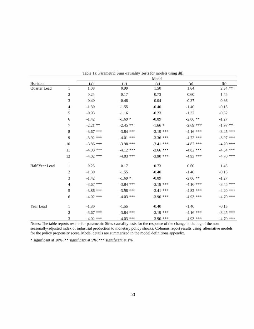
HorizonQuarter Lead 1 1.08 0.99 1.50 1.64 2.34 **
2 0.25 0.17 0.73 0.60 1.453 -0.40 -0.48 0.04 -0.37 0.364 -1.30 -1.55 -0.40 -1.40 -0.155 -0.93 -1.16 -0.23 -1.32 -0.326 -1.42 -1.69 * -0.89 -2.06 ** -1.277 -2.21 ** -2.45 ** -1.66 * -2.69 *** -1.97 **8 -3.67 *** -3.84 *** -3.19 *** -4.16 *** -3.45 ***9 -3.92 *** -4.01 *** -3.36 *** -4.72 *** -3.97 ***
10 -3.86 *** -3.98 *** -3.41 *** -4.82 *** -4.20 ***11 -4.03 *** -4.12 *** -3.66 *** -4.82 *** -4.34 ***12 -4.02 *** -4.03 *** -3.90 *** -4.93 *** -4.70 ***
Half Year Lead 1 0.25 0.17 0.73 0.60 1.452 -1.30 -1.55 -0.40 -1.40 -0.153 -1.42 -1.69 * -0.89 -2.06 ** -1.274 -3.67 *** -3.84 *** -3.19 *** -4.16 *** -3.45 ***5 -3.86 *** -3.98 *** -3.41 *** -4.82 *** -4.20 ***6 -4.02 *** -4.03 *** -3.90 *** -4.93 *** -4.70 ***
Year Lead 1 -1.30 -1.55 -0.40 -1.40 -0.152 -3.67 *** -3.84 *** -3.19 *** -4.16 *** -3.45 ***3 -4.02 *** -4.03 *** -3.90 *** -4.93 *** -4.70 ***
* significant at 10%; ** significant at 5%; *** significant at 1%
Notes: The table reports results for parametric Sims-causality tests for the response of the change in the log of the non-seasonally-adjusted index of industrial production to monetary policy shocks. Columns report results using alternative models for the policy propensity score. Model details are summarized in the model definitions appendix.
Table 1a: Parametric Sims-causality Tests for models using dfft-1
Model (a) (b) (c) (g) (h)
53
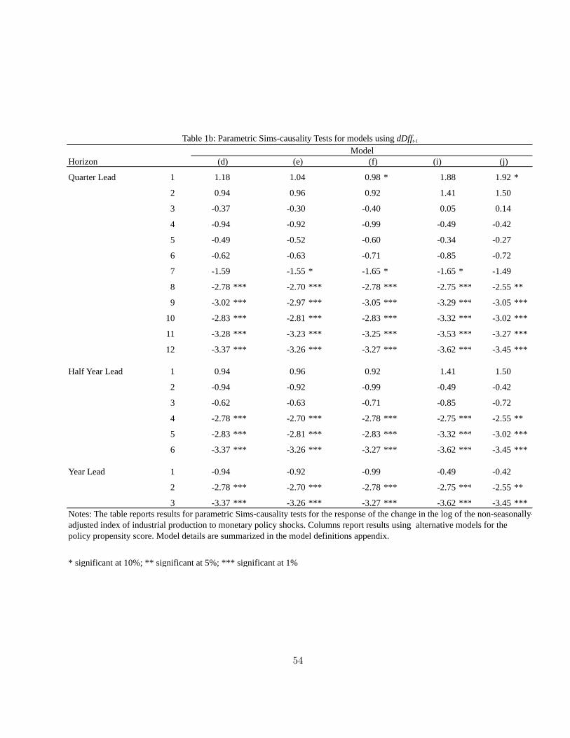
Horizon (i)
Quarter Lead 1 1.18 1.04 0.98 * 1.88 1.92 *
2 0.94 0.96 0.92 1.41 1.50
3 -0.37 -0.30 -0.40 0.05 0.14
4 -0.94 -0.92 -0.99 -0.49 -0.42
5 -0.49 -0.52 -0.60 -0.34 -0.27
6 -0.62 -0.63 -0.71 -0.85 -0.72
7 -1.59 -1.55 * -1.65 * -1.65 * -1.49
8 -2.78 *** -2.70 *** -2.78 *** -2.75 *** -2.55 **
9 -3.02 *** -2.97 *** -3.05 *** -3.29 *** -3.05 ***
10 -2.83 *** -2.81 *** -2.83 *** -3.32 *** -3.02 ***
11 -3.28 *** -3.23 *** -3.25 *** -3.53 *** -3.27 ***
12 -3.37 *** -3.26 *** -3.27 *** -3.62 *** -3.45 ***
Half Year Lead 1 0.94 0.96 0.92 1.41 1.50
2 -0.94 -0.92 -0.99 -0.49 -0.42
3 -0.62 -0.63 -0.71 -0.85 -0.72
4 -2.78 *** -2.70 *** -2.78 *** -2.75 *** -2.55 **
5 -2.83 *** -2.81 *** -2.83 *** -3.32 *** -3.02 ***
6 -3.37 *** -3.26 *** -3.27 *** -3.62 *** -3.45 ***
Year Lead 1 -0.94 -0.92 -0.99 -0.49 -0.42
2 -2.78 *** -2.70 *** -2.78 *** -2.75 *** -2.55 **
3 -3.37 *** -3.26 *** -3.27 *** -3.62 *** -3.45 ***
* significant at 10%; ** significant at 5%; *** significant at 1%
Notes: The table reports results for parametric Sims-causality tests for the response of the change in the log of the non-seasonally-adjusted index of industrial production to monetary policy shocks. Columns report results using alternative models for the policy propensity score. Model details are summarized in the model definitions appendix.
Table 1b: Parametric Sims-causality Tests for models using dDfft-1
(d) (e) (f) (j)Model
54
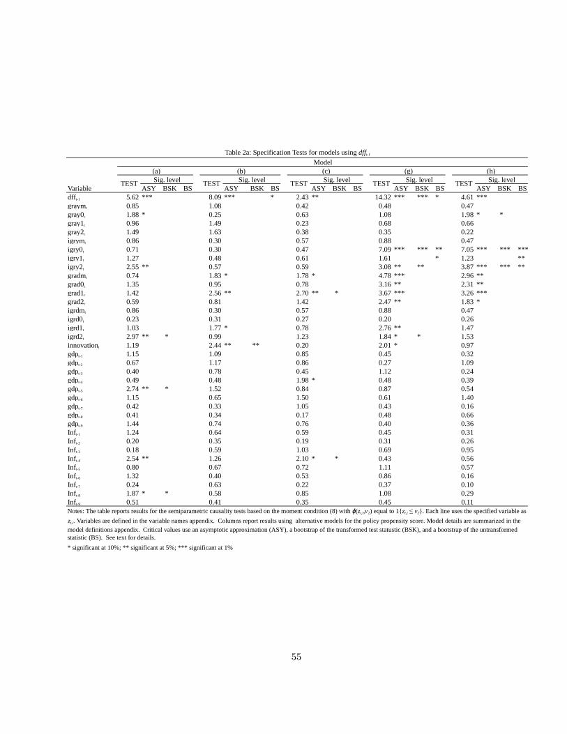
Variable ASY BSK BS ASY BSK BS ASY BSK BS ASY BSK BS ASY BSK BSdfft-1 5.62 *** 8.09 *** * 2.43 ** 14.32 *** *** * 4.61 ***graymt 0.85 1.08 0.42 0.48 0.47gray0t 1.88 * 0.25 0.63 1.08 1.98 * *gray1t 0.96 1.49 0.23 0.68 0.66gray2t 1.49 1.63 0.38 0.35 0.22igrymt 0.86 0.30 0.57 0.88 0.47igry0t 0.71 0.30 0.47 7.09 *** *** ** 7.05 *** *** ***igry1t 1.27 0.48 0.61 1.61 * 1.23 **igry2t 2.55 ** 0.57 0.59 3.08 ** ** 3.87 *** *** **gradmt 0.74 1.83 * 1.78 * 4.78 *** 2.96 **grad0t 1.35 0.95 0.78 3.16 ** 2.31 **grad1t 1.42 2.56 ** 2.70 ** * 3.67 *** 3.26 ***grad2t 0.59 0.81 1.42 2.47 ** 1.83 *igrdmt 0.86 0.30 0.57 0.88 0.47igrd0t 0.23 0.31 0.27 0.20 0.26igrd1t 1.03 1.77 * 0.78 2.76 ** 1.47igrd2t 2.97 ** * 0.99 1.23 1.84 * * 1.53innovationt 1.19 2.44 ** ** 0.20 2.01 * 0.97gdpt-1 1.15 1.09 0.85 0.45 0.32gdpt-2 0.67 1.17 0.86 0.27 1.09gdpt-3 0.40 0.78 0.45 1.12 0.24gdpt-4 0.49 0.48 1.98 * 0.48 0.39gdpt-5 2.74 ** * 1.52 0.84 0.87 0.54gdpt-6 1.15 0.65 1.50 0.61 1.40gdpt-7 0.42 0.33 1.05 0.43 0.16gdpt-8 0.41 0.34 0.17 0.48 0.66gdpt-9 1.44 0.74 0.76 0.40 0.36Inft-1 1.24 0.64 0.59 0.45 0.31Inft-2 0.20 0.35 0.19 0.31 0.26Inft-3 0.18 0.59 1.03 0.69 0.95Inft-4 2.54 ** 1.26 2.10 * * 0.43 0.56Inft-5 0.80 0.67 0.72 1.11 0.57Inft-6 1.32 0.40 0.53 0.86 0.16Inft-7 0.24 0.63 0.22 0.37 0.10Inft-8 1.87 * * 0.58 0.85 1.08 0.29Inft-9 0.51 0.41 0.35 0.45 0.11
* significant at 10%; ** significant at 5%; *** significant at 1%
Sig. level
Table 2a: Specification Tests for models using dfft-1
Model (a) (b) (c) (g) (h)
Notes: The table reports results for the semiparametric causality tests based on the moment condition (8) with !(zt,i,v2) equal to 1{zt,i ! v2}. Each line uses the specified variable as zt,i. Variables are defined in the variable names appendix. Columns report results using alternative models for the policy propensity score. Model details are summarized in the model definitions appendix. Critical values use an asymptotic approximation (ASY), a bootstrap of the transformed test statustic (BSK), and a bootstrap of the untransformed statistic (BS). See text for details.
TEST Sig. level TEST Sig. levelTEST Sig. level TEST Sig. level TEST
55
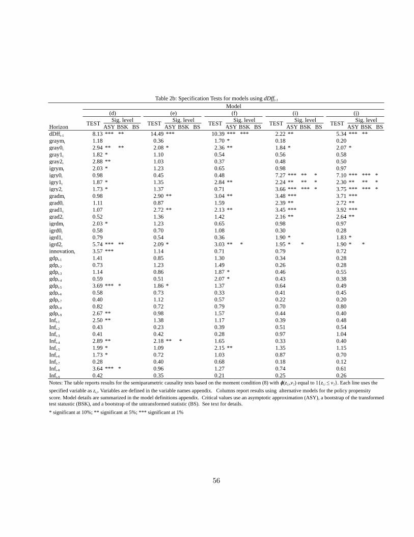
Horizon ASY BSK BS ASY BSK BS ASY BSK BS ASY BSK BS ASY BSK BSdDfft-1 8.13 *** ** 14.49 *** 10.39 *** *** 2.22 ** 5.34 *** **graymt 1.18 0.36 1.70 * 0.18 0.20gray0t 2.94 ** ** 2.08 * 2.36 ** 1.84 * 2.07 *gray1t 1.82 * 1.10 0.54 0.56 0.58gray2t 2.88 ** 1.03 0.37 0.48 0.50igrymt 2.03 * 1.23 0.65 0.98 0.97igry0t 0.98 0.45 0.48 7.27 *** ** * 7.10 *** *** *igry1t 1.87 * 1.35 2.84 ** 2.24 ** ** * 2.30 ** ** *igry2t 1.73 * 1.37 0.71 3.66 *** *** * 3.75 *** *** *gradmt 0.98 2.90 ** 3.04 ** 3.48 *** 3.71 ***grad0t 1.11 0.87 1.59 2.39 ** 2.72 **grad1t 1.07 2.72 ** 2.13 ** 3.45 *** 3.92 ***grad2t 0.52 1.36 1.42 2.16 ** 2.64 **igrdmt 2.03 * 1.23 0.65 0.98 0.97igrd0t 0.58 0.70 1.08 0.30 0.28igrd1t 0.79 0.54 0.36 1.90 * 1.83 *igrd2t 5.74 *** ** 2.09 * 3.03 ** * 1.95 * * 1.90 * *innovationt 3.57 *** 1.14 0.71 0.79 0.72gdpt-1 1.41 0.85 1.30 0.34 0.28gdpt-2 0.73 1.23 1.49 0.26 0.28gdpt-3 1.14 0.86 1.87 * 0.46 0.55gdpt-4 0.59 0.51 2.07 * 0.43 0.38gdpt-5 3.69 *** * 1.86 * 1.37 0.64 0.49gdpt-6 0.58 0.73 0.33 0.41 0.45gdpt-7 0.40 1.12 0.57 0.22 0.20gdpt-8 0.82 0.72 0.79 0.70 0.80gdpt-9 2.67 ** 0.98 1.57 0.44 0.40Inft-1 2.50 ** 1.38 1.17 0.39 0.48Inft-2 0.43 0.23 0.39 0.51 0.54Inft-3 0.41 0.42 0.28 0.97 1.04Inft-4 2.89 ** 2.18 ** * 1.65 0.33 0.40Inft-5 1.99 * 1.09 2.15 ** 1.35 1.15Inft-6 1.73 * 0.72 1.03 0.87 0.70Inft-7 0.28 0.40 0.68 0.18 0.12Inft-8 3.64 *** * 0.96 1.27 0.74 0.61Inft-9 0.42 0.35 0.21 0.25 0.26
* significant at 10%; ** significant at 5%; *** significant at 1%
Sig. level TESTSig. level TEST Sig. level TEST Sig. level TEST Sig. level
Notes: The table reports results for the semiparametric causality tests based on the moment condition (8) with !(zt,i,v2) equal to 1{zt,i ! v2}. Each line uses the specified variable as zt,i. Variables are defined in the variable names appendix. Columns report results using alternative models for the policy propensity score. Model details are summarized in the model definitions appendix. Critical values use an asymptotic approximation (ASY), a bootstrap of the transformed test statustic (BSK), and a bootstrap of the untransformed statistic (BS). See text for details.
Table 2b: Specification Tests for models using dDfft-1
Model (d) (e) (f) (i) (j)
TEST
56
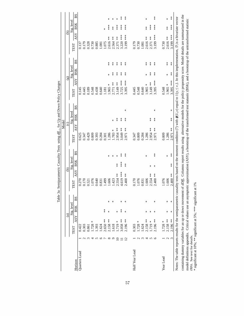
Hor
izon
ASY
BSK
BS
ASY
BSK
BS
ASY
BSK
BS
ASY
BSK
BS
ASY
BSK
BS
Qua
rters
Lea
d 1
0.42
20.
270
0.62
50.
145
0.13
7
20.
303
0.17
00.
347
0.44
50.
179
3
0.86
10.
521
0.42
90.
189
0.32
8
41.
728
*1.
076
0.80
90.
548
0.73
0
51.
393
0.64
00.
393
0.43
80.
885
6
1.62
40.
831
0.28
40.
640
1.08
1
72.
650
****
1.49
90.
301
1.18
11.
075
*
82.
158
***
*1.
606
*1.
286
1.96
5*
***
2.61
6**
***
*
91.
618
*1.
423
*1.
783
**
2.77
1**
****
2.56
4**
***
10
1.71
9*
*2.
554
****
*2.
954
****
3.14
9**
****
2.37
1**
***
*
113.
058
****
*4.
619
***
***
**3.
049
****
3.72
5**
***
**3.
220
***
***
**
122.
196
***
*2.
400
****
**2.
971
****
*3.
395
***
****
3.19
9**
***
***
Hal
f Yea
r Lea
d1
0.30
30.
170
0.34
70.
445
0.17
9
21.
728
*1.
076
0.80
90.
548
0.73
0
31.
624
0.83
10.
284
0.64
01.
081
4
2.15
8**
**
1.60
6*
1.28
61.
965
**
**2.
616
****
*
51.
719
**
2.55
4**
*2.
954
****
3.14
9**
****
2.37
1**
***
6
2.19
6**
**
2.40
0**
***
2.97
1**
***
3.39
5**
***
**3.
199
***
***
** Ye
ar L
ead
11.
728
*1.
076
0.80
90.
548
0.73
0
22.
158
***
*1.
606
*1.
286
1.96
5*
***
2.61
6**
***
3
2.19
6**
**
2.40
0**
****
2.97
1**
***
3.39
5**
***
**3.
199
***
***
**
* si
gnifi
cant
at 1
0%; *
* si
gnifi
cant
at 5
%; *
** si
gnifi
cant
at 1
%
Tabl
e 3a
: Sem
ipar
amet
ric C
ausa
lity
Test
s us
ing
dff
t-1, f
or U
p an
d D
own
Polic
y C
hang
esM
odel
TEST
Sig.
leve
lTE
STSi
g. le
vel
Sig.
leve
lTE
STTE
STSi
g. le
vel
Not
es: T
he ta
ble
repo
rts re
sults
for t
he se
mip
aram
etric
cau
salit
y te
sts b
ased
on
the
mom
ent c
ondi
tion
(7) w
ith !
(Ut,v
) equ
al to
1{y
t ! v
1}. I
n th
is im
plem
enta
tion,
Dt is
a b
ivar
iate
vec
tor
cont
aini
ng d
umm
y va
riabl
es fo
r an
up o
r dow
n m
ovem
ent o
f dD
fft.
Col
umns
repo
rt re
sults
usi
ng a
ltern
ativ
e m
odel
s for
the
polic
y pr
open
sity
scor
e. M
odel
det
ails
are
sum
mar
ized
in th
e m
odel
def
initi
ons a
ppen
dix.
Crit
ical
val
ues u
se a
n as
ympt
otic
app
roxi
mat
ion
(ASY
), a
boot
stra
p of
the
trans
form
ed te
st st
atus
tic (B
SK),
and
a bo
otst
rap
of th
e un
trans
form
ed st
atis
tic
(BS)
. Se
e te
xt fo
r det
ails
.
(a)
(b)
(c)
(g)
(h)
TEST
Sig.
leve
l
57
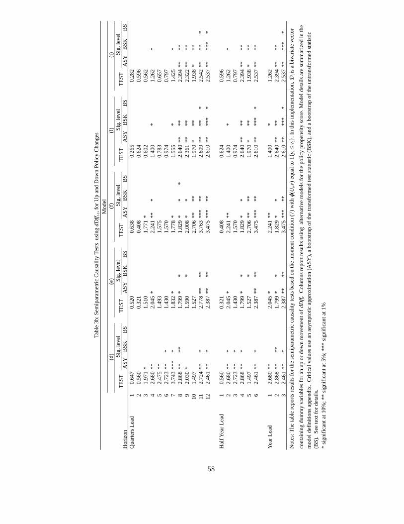
Hor
izon
ASY
BSK
BS
ASY
BSK
BS
ASY
BSK
BS
ASY
BSK
BS
ASY
BSK
BS
Qua
rters
Lea
d 1
0.64
70.
520
0.63
80.
265
0.28
2
20.
560
0.32
10.
408
0.62
40.
596
3
1.97
1*
1.51
01.
771
*0.
602
0.56
2
42.
680
**2.
045
*2.
241
***
1.40
0*
1.26
2*
5
2.47
5**
1.49
31.
575
0.78
30.
657
6
2.72
3**
*1.
430
1.57
00.
974
0.79
7
73.
743
***
*1.
832
*1.
778
*1.
555
*1.
425
*
82.
868
****
1.79
9*
*1.
829
**
*2.
640
****
2.39
4**
**
92.
030
*1.
590
*2.
008
**
2.36
1**
**2.
322
****
10
1.49
71.
527
2.70
6**
**1.
970
***
1.93
8*
**
112.
724
***
2.77
8**
**3.
763
***
**2.
609
****
*2.
542
****
*
122.
461
***
2.38
7**
**3.
475
***
**2.
610
****
**
2.53
7**
***
* H
alf Y
ear L
ead
10.
560
0.32
10.
408
0.62
40.
596
2
2.68
0**
*2.
045
*2.
241
**1.
400
*1.
262
*
32.
723
***
1.43
01.
570
0.97
40.
797
4
2.86
8**
*1.
799
**
1.82
9*
*2.
640
****
2.39
4**
**
51.
497
1.52
7*
2.70
6**
**1.
970
***
1.93
8*
**
62.
461
***
2.38
7**
**3.
475
***
**2.
610
****
**
2.53
7**
** Ye
ar L
ead
12.
680
**2.
045
*2.
241
**1.
400
*1.
262
2
2.86
8**
**1.
799
**
1.82
9*
*2.
640
****
2.39
4**
**
32.
461
***
2.38
7**
**3.
475
***
**2.
610
****
**
2.53
7**
***
*
* si
gnifi
cant
at 1
0%; *
* si
gnifi
cant
at 5
%; *
** si
gnifi
cant
at 1
%
Tabl
e 3b
: Sem
ipar
amet
ric C
ausa
lity
Test
s us
ing
dD
fft-
1, f
or U
p an
d D
own
Polic
y C
hang
esM
odel
TEST
Sig.
leve
lTE
STSi
g. le
vel
TEST
Sig.
leve
lTE
STSi
g. le
vel
Not
es: T
he ta
ble
repo
rts re
sults
for t
he se
mip
aram
etric
cau
salit
y te
sts b
ased
on
the
mom
ent c
ondi
tion
(7) w
ith !
(Ut,v
) equ
al to
1{y
t ! v
1}. I
n th
is im
plem
enta
tion,
Dt is
a b
ivar
iate
vec
tor
cont
aini
ng d
umm
y va
riabl
es fo
r an
up o
r dow
n m
ovem
ent o
f dD
fft.
Col
umns
repo
rt re
sults
usi
ng a
ltern
ativ
e m
odel
s for
the
polic
y pr
open
sity
scor
e. M
odel
det
ails
are
sum
mar
ized
in th
e m
odel
def
initi
ons a
ppen
dix.
Crit
ical
val
ues u
se a
n as
ympt
otic
app
roxi
mat
ion
(ASY
), a
boot
stra
p of
the
trans
form
ed te
st st
atus
tic (B
SK),
and
a bo
otst
rap
of th
e un
trans
form
ed st
atis
tic
(BS)
. Se
e te
xt fo
r det
ails
.
(d)
(e)
(f)
(i)
(j)
TEST
Sig.
leve
l
58
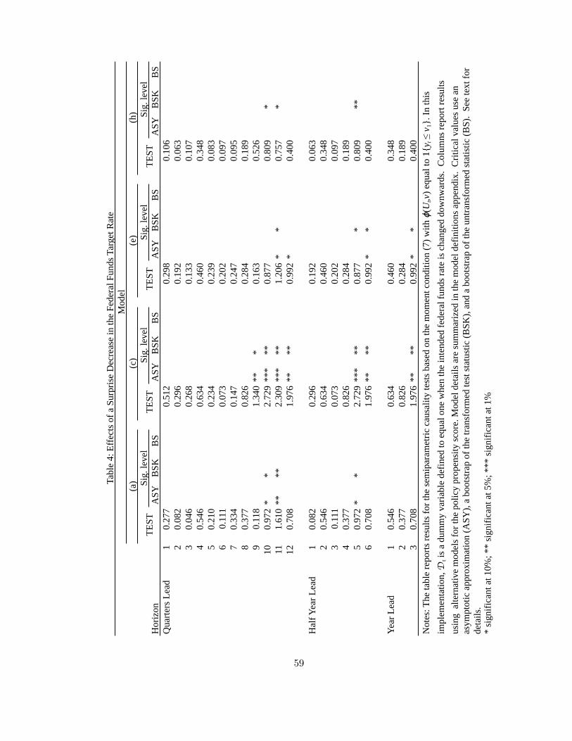
Hor
izon
ASY
BSK
BS
ASY
BSK
BS
ASY
BSK
BS
ASY
BSK
BS
Qua
rters
Lea
d 1
0.27
70.
512
0.29
80.
106
2
0.08
20.
296
0.19
20.
063
3
0.04
60.
268
0.13
30.
107
4
0.54
60.
634
0.46
00.
348
5
0.21
00.
234
0.23
90.
083
6
0.11
10.
073
0.20
20.
097
7
0.33
40.
147
0.24
70.
095
8
0.37
70.
826
0.28
40.
189
9
0.11
81.
340
***
0.16
30.
526
10
0.97
2*
*2.
729
***
**0.
877
0.80
9*
11
1.61
0**
**2.
309
***
**1.
206
**
0.75
7*
12
0.70
81.
976
****
0.99
2*
0.40
0 H
alf Y
ear L
ead
10.
082
0.29
60.
192
0.06
3
20.
546
0.63
40.
460
0.34
8
30.
111
0.07
30.
202
0.09
7
40.
377
0.82
60.
284
0.18
9
50.
972
**
2.72
9**
***
0.87
7*
0.80
9**
6
0.70
81.
976
****
0.99
2*
*0.
400
Year
Lea
d
1
0.54
60.
634
0.46
00.
348
2
0.37
70.
826
0.28
40.
189
3
0.70
81.
976
****
0.99
2*
*0.
400
* si
gnifi
cant
at 1
0%; *
* si
gnifi
cant
at 5
%; *
** si
gnifi
cant
at 1
%
Sig.
leve
l
Not
es: T
he ta
ble
repo
rts re
sults
for t
he se
mip
aram
etric
cau
salit
y te
sts b
ased
on
the
mom
ent c
ondi
tion
(7) w
ith !
(Ut,v
) equ
al to
1{y
t ! v
1}. I
n th
is
impl
emen
tatio
n, D
t is a
dum
my
varia
ble
defin
ed to
equ
al o
ne w
hen
the
inte
nded
fede
ral f
unds
rate
is c
hang
ed d
ownw
ards
. C
olum
ns re
port
resu
lts
usin
g a
ltern
ativ
e m
odel
s for
the
polic
y pr
open
sity
scor
e. M
odel
det
ails
are
sum
mar
ized
in th
e m
odel
def
initi
ons a
ppen
dix.
Crit
ical
val
ues u
se a
n as
ympt
otic
app
roxi
mat
ion
(ASY
), a
boot
stra
p of
the
trans
form
ed te
st st
atus
tic (B
SK),
and
a bo
otst
rap
of th
e un
trans
form
ed st
atis
tic (B
S).
See
text
for
deta
ils.
TEST
Sig.
leve
lTE
STSi
g. le
vel
TEST
Sig.
leve
lTE
ST
Tabl
e 4:
Effe
cts o
f a S
urpr
ise
Dec
reas
e in
the
Fede
ral F
unds
Tar
get R
ate
(a)
(c)
(e)
(h)
Mod
el
59
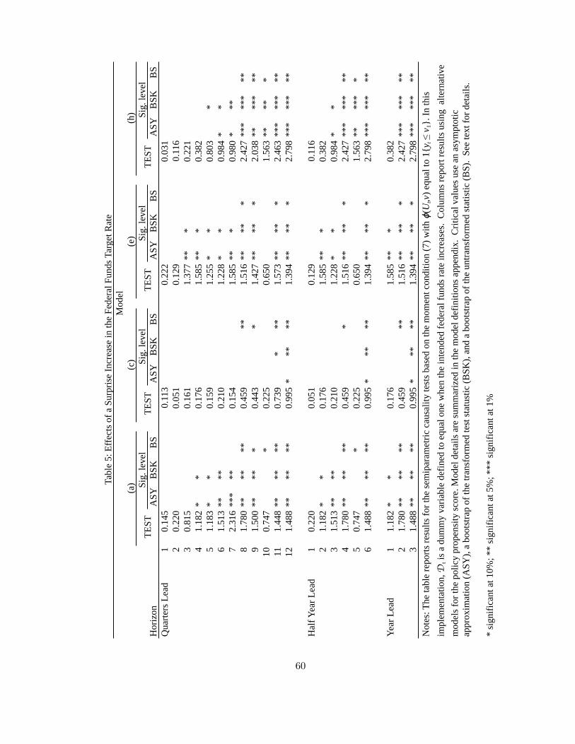
Hor
izon
ASY
BSK
BS
ASY
BSK
BS
ASY
BSK
BS
ASY
BSK
BS
Qua
rters
Lea
d 1
0.14
50.
113
0.22
20.
031
2
0.22
00.
051
0.12
90.
116
3
0.81
50.
161
1.37
7**
*0.
221
4
1.18
2*
*0.
176
1.58
5**
*0.
382
5
1.18
3*
*0.
159
1.25
5*
*0.
803
*
61.
513
****
0.21
01.
228
**
0.98
4*
*
72.
316
***
**0.
154
1.58
5**
*0.
980
***
8
1.78
0**
****
0.45
9**
1.51
6**
***
2.42
7**
***
***
9
1.50
0**
***
0.44
3*
1.42
7**
***
2.03
8**
***
**
100.
747
*0.
225
0.65
01.
563
****
*
111.
448
****
**0.
739
***
1.57
3**
***
2.46
3**
***
***
12
1.48
8**
****
0.99
5*
****
1.39
4**
***
2.79
8**
***
***
Hal
f Yea
r Lea
d1
0.22
00.
051
0.12
90.
116
2
1.18
2*
*0.
176
1.58
5**
*0.
382
3
1.51
3**
**0.
210
1.22
8*
*0.
984
**
4
1.78
0**
****
0.45
9*
1.51
6**
***
2.42
7**
***
***
5
0.74
7*
0.22
50.
650
1.56
3**
***
*
61.
488
****
**0.
995
***
**1.
394
****
*2.
798
***
***
** Ye
ar L
ead
11.
182
**
0.17
61.
585
***
0.38
2
21.
780
****
**0.
459
**1.
516
****
*2.
427
***
***
**
31.
488
****
**0.
995
***
**1.
394
****
*2.
798
***
***
**
* si
gnifi
cant
at 1
0%; *
* si
gnifi
cant
at 5
%; *
** si
gnifi
cant
at 1
%
Sig.
leve
l
Not
es: T
he ta
ble
repo
rts re
sults
for t
he se
mip
aram
etric
cau
salit
y te
sts b
ased
on
the
mom
ent c
ondi
tion
(7) w
ith !
(Ut,v
) equ
al to
1{y
t ! v
1}. I
n th
is
impl
emen
tatio
n, D
t is a
dum
my
varia
ble
defin
ed to
equ
al o
ne w
hen
the
inte
nded
fede
ral f
unds
rate
incr
ease
s. C
olum
ns re
port
resu
lts u
sing
alte
rnat
ive
mod
els f
or th
e po
licy
prop
ensi
ty sc
ore.
Mod
el d
etai
ls a
re su
mm
ariz
ed in
the
mod
el d
efin
ition
s app
endi
x. C
ritic
al v
alue
s use
an
asym
ptot
ic
appr
oxim
atio
n (A
SY),
a bo
otst
rap
of th
e tra
nsfo
rmed
test
stat
ustic
(BSK
), an
d a
boot
stra
p of
the
untra
nsfo
rmed
stat
istic
(BS)
. Se
e te
xt fo
r det
ails
.
TEST
Sig.
leve
lTE
STSi
g. le
vel
TEST
Sig.
leve
lTE
ST
Tabl
e 5:
Effe
cts o
f a S
urpr
ise
Incr
ease
in th
e Fe
dera
l Fun
ds T
arge
t Rat
e
(a)
(c)
(e)
(h)
Mod
el
60
References
Abadie, A. (2002): �Bootstrap Tests for Distributional Treatment E¤ects in Instrumental Variables
Models,�Journal of the American Statistical Association, pp. 284�292.
(2005): �Semiparametric Di¤erence-in-Di¤erences Estimators,� Review of Economic Studies,
72(1), 1�19.
Andrews, D. W. (1995): �Nonparametric Kernel Estimation for Semiparametric Models,�Econometric
Theory, pp. 560�596.
Arcones, M. A., and B. Yu (1994): �Central Limit Theorems for Empirical and U-Processes of Sta-
tionary Mixing Sequences,�Journal of Theoretical Probability, pp. 47�71.
Bai, J. (2002): �Testing Parametric Conditional Distributions of Dynamic Models,�mimeo.
Bernanke, B. S., and A. S. Blinder (1992): �The Federal Funds Rate and the Channels of Monetary
Transmission,�The American Economic Review, 82, 901�921.
Bernanke, B. S., and J. Boivin (2003): �Monetary Policy in a Data-Rich Environment,� Journal of
Monetary Economics, 50, 525�546.
Bernanke, B. S., J. Boivin, and P. Eliasz (2005): �Measuring the E¤ects of Monetary Policy: A
Factor-Augmented Vector Autoregressive (FAVAR) Approach,�The Quarterly Journal of Economics,
pp. 387�422.
Bernanke, B. S., and I. Mihov (1998): �Measuring Monetary Policy,� The Quarterly Journal of
Economics, 113, 869�902.
Bierens, H. J. (1982): �Consistent Model Speci�cation Tests,�Journal of Econometrics, 20, 105�134.
(1987): �Kernel Estimators of Regression Functions,�in Advances in Econometrics: Fifth World
Congress, ed. by T. Bewley, pp. 99�144. Cambridge University Press, New York.
(1990): �A consistent conditional moment test of functional form.,�Econometrica, 58, 1443�1458.
Bierens, H. J., and W. Ploberger (1997): �Asymptotic theory of integrated conditional moment
tests,�Econometrica, 65, 1129�1152.
Blanchard, O. J., and C. M. Kahn (1980): �The Solution of Linear Di¤erence Models under Rational
Expectations,�Econometrica, 48, 1305�1311.
61
Chamberlain, G. (1982): �The General Equivalence of Granger and Sims Causality,�Econometrica, pp.
569�581.
Chen, X., and Y. Fan (1999): �Consistent hypothesis testing in semiparametric and nonparametric
models for econometric time series,�Journal of Econometrics, 91, 373�401.
Christiano, L., M. Eichenbaum, and C. L. Evans (1999): �Monetary Policy Shocks: What Have
We Learned And To What End?,�in Handbook of Macroeconomics, Volume 1, ed. by J. B. Taylor, and
M. Woodford, chap. 2, pp. 65�148. Elsevier Science B.V.
Christiano, L. J., M. Eichenbaum, and C. Evans (1996): �The E¤ects of Monetary Policy Shocks:
Evidence from the Flow of Funds,�The Review of Economics and Statistics, 78, 16�34.
Clarida, R., J. Gali, and M. Gertler (2000): �Monetary Policy Rules and Macroeconomic Stability:
Evidence and some Theory,�The Quarterly Journal of Economics, pp. 147�180.
Cochrane, J. H. (1994): �Shocks,�Carnegie-Rochester Conference Series on Public Policy, 41, 295�364.
Dehejia, R. H., and S. Wahba (1999): �Causal E¤ects in Nonexperimental Studies: Reevaluating the
Evaluation of Training Programs,�Journal of the American Statistical Association, 94, 1053�1062.
Delgado, M. A., and W. Stute (2005): �Distribution Free Speci�cation Tests of Conditional Models,�
manuscript.
Dufour, J.-M., and E. Renault (1998): �Short Run and Long Run Causality in Time Series: Theory,�
Econometrica, pp. 1099�1125.
Dufour, J.-M., and D. Tessier (1993): �On the relationship between impulse response analysis, inno-
vation accounting and Granger causality,�Economics Letters, 42, 327�333.
Eichengreen, B., M. W. Watson, and R. S. Grossman (1985): �Bank Rate Policy Under the Interwar
Gold Standard: A Dynamic Probit Model,�The Economic Journal, 95, 725�745.
Florens, J.-P., and M. Mouchart (1982): �A Note on Non-Causality,�Econometrica, pp. 582�591.
Florens, J.-P., and M. Mouchart (1985): �A Linear Theory for Noncausality,� Econometrica, pp.
157�176.
Genberg, H., and S. Gerlach (2004): �Estimating Central Bank Reaction Function with Ordered
Probit: A Note,�mimeo.
62
Gordon, D. B., and E. M. Leeper (1994): �The Dynamic Impacts of Monetary Policy: An Exercise
in Tentative Identi�cation,�The Journal of Political Economy, 102, 1228�1247.
Hahn, J. (1999): �How informative is the initial condition in the dynamic panel model with �xed e¤ects,�
Journal of Econometrics, 93, 309�326.
Hall, P., and C. Heyde (1980): Martingale Limit Theory and its Application. Academic Press.
Hamilton, J. D., and O. Jorda (2002): �A Model of the Federal Funds Rate Target,� Journal of
Political Economy, pp. 1135�1167.
Hansen, B. E. (1996): �Inference when a nuisance parameter is not identi�ed under the null hypothesis.,�
Econometrica, 64, 413�430.
Heckman, J. J., H. Ichimura, and P. E. Todd (1997): �Matching as an Econometric Evaluation
Estimator: Evidence from Evaluating a Job Training Programme,� Review of Economic Studies, 64,
605�654.
Heckman, J. J., H. Ichimura, and P. E. Todd (1998): �Matching as an Econometric Evaluation
Estimator,�Review of Economic Studies, 65, 261�294.
Hirano, K., and G. Imbens (2004): �The Propensity Score with Continuous Treatments,� Berkeley
Department of Economics, mimeo.
Hirano, K., G. Imbens, and G. Ridder (2003a): �E¢ cient Estimation of Average Treatment E¤ects
using the Estimated Propensity Score,�Econometrica, 71, 1161�1189.
Hirano, K., G. Imbens, and G. Ridder (2003b): �E¢ cient Estimation of Average Treatment E¤ects
using the Estimated Propensity Score,�Econometrica, 71, 1161�1189.
Hu, L., and P. C. Phillips (2002a): �Dynamics of the Federal Funds Target Rate: A Nonstationary
Discrete Choice Approach,�Cowles Foundation Discussion Paper No. 1365.
(2002b): �Nonstationary Discrete Choice,�Cowles Foundation Discussion Paper No 1364.
Imbens, G. W. (2000): �The Role of the Propensity Score in Estimating Dose-Response Functions,�
Biometrika, 87, 706�710.
Khmaladze, E. (1981): �Martingale Approach in the Theory of Goodness-of-�t Tests,�Theory of Prob-
ability and Its Applications, pp. 240�257.
63
(1988): �An Innovation Approach to Goodness-of-Fit Tests in Rm,� Annals of Statistics, pp.
1503�1516.
Khmaladze, E. V. (1993): �Goodness of Fit Problem and Scanning Innovation Martingales,�The Annals
of Statistics, pp. 789�829.
Koenker, R., and Z. Xiao (2002): �Inference of the Quantile Regression Process,�Econometrica, 70,
1583�1612.
Koul, H. L., andW. Stute (1999): �Nonparametric Model Checks for Time Series,�Annals of Statistics,
pp. 204�236.
Lechner, M. (2000): �Identi�cation and Estimation of Causal E¤ects of Multiple Treatments under the
Conditional Independence Assumption,� in Economic Evaluations of Active Labour Market Policies in
Europe, ed. by M. Lechner, and F. Pfei¤er. Physica, Heidelberg.
Lechner, M. (2004): �Sequential Matching Estimation of Dynamic Causal Models,�Discussion Paper
2004-06, Department of Economics, University of St. Gallen.
Leeper, E. M. (1997): �Narrative and VAR approaches to Monetary Policy: Common Identi�cation
Problems,�Journal of Monetary Economics, pp. 641�657.
Leeper, E. M., C. A. Sims, and T. Zha (1996): �What Does Monetary Policy Do?,�Brookings Papers
on Economic Activity, 1996, 1�78.
Linton, O., and P. Gozalo (1999): �Conditional Independence Restrictions: Testing and Estimation,�
mimeo.
Lok, J., R. Gill, A. V. der Vaart, and J. Robins (2004): �Estimating the causal e¤ect of a time-
varying treatment on time-to-event using structural nested failure time models,�Statistica Neerlandica,
58, 271�295.
Lubik, T. A., and F. Schorfheide (2003): �Computing sunspot equilibria in linear rational expectations
models,�Journal of Economic Dynamics and Control, 28, 273�285.
(2004): �Testing for Indeterminacy: An Application to U.S. Monetary Policy,�The American
Economic Review, 94, 190�217.
Mammen, E. (1993): �Bootstrap and the Wild Bootstrap for High Dimensional Linear Models,�Annals
of Statistics, 21, 255�285.
64
Moench, E., and H. Uhlig (2005): �Towards a Monthly Business Cycle Chronology for the Euro Area,�
Journal of Business Cycle Measurement and Analysis, 2, 43�69.
Pakes, A., and D. Pollard (1989): �Simulation and the Asymptotics of Optimization Estimators,�
Econometrica, 57(5), 1027�1057.
Park, J. Y., and P. C. Phillips (2000): �Nonstationary Binary Choice,�Econometrica, pp. 1249�1280.
Pollard, D. (1984): Convergence of Stochastic Processes. Springer-Verlag New York, Inc.
Robins, J. M., S. Greenland, and F.-C. Hu (1999): �Estimation of the Causal E¤ect of a Time-
Varying Exposure on the Marginal Mean of a Repeated Binary Outcome,� Journal of the American
Statistical Association, pp. 687�712.
Romer, C. D., and D. H. Romer (2004): �A New Measure of Monetary Shocks: Derivation and
Implications,�The American Economic Review, 94, 1055�1084.
Rosenbaum, P. R., and D. B. Rubin (1983): �The Central Role of the Propensity Score in Observational
Studies for Causal E¤ects,�Biometrika, pp. 41�55.
Rosenblatt, M. (1952): �Remarks on a Multivariate Transform,�The Annals of Mathematical Statistics,
23(3), 470�472.
Rotemberg, J. J., and M. Woodford (1997): �An Optimization-Based Econometric Framework for
the Evaluation of Monetary Policy,�NBER Macroeconomic Annual, 12, 297�346.
Rubin, D. B. (1974): �Estimating Causal E¤ects of Treatments in Randomized and Non-Randomized
Studies,�Journal of Educational Psychology, pp. 688�701.
(1978): �Bayesian Inference for Causal E¤ects: The Role of Randomization,� The Annals of
Statistics, 6, 34�58.
Shapiro, M. D. (1994): �Federal Reserve Policy: Cause and E¤ect,� in Monetary Policy, ed. by G. N.
Mankiew, pp. 307�334. University of Chicago Press.
Sims, C., and T. Zha (2006): �Does Monetary Policy Generate Recessions,�Macroeconomic Dynamics,
10, 231�272.
Sims, C. A. (1972): �Money, Income and Causality,�American Economic Review, pp. 540�562.
(1980): �Macroeconomics and Reality,�Econometrica, pp. 1�48.
65
(2001): �Solving Linear Rational Expectations Models,�Computational Economics, 20, 1�20.
Stock, J. H., and M. W. Watson (2002a): �Forecasting Using Principle Components from a Large
Number of Predictors,�Journal of the American Statistical Association, 97, 1167�1179.
(2002b): �Macroeconomic Forecasting Using Di¤usion Indexes,� Journal of Business and Eco-
nomic Statistics, 20, 147�162.
Strongin, S. (1995): �The Identi�cation of Monetary Policy Disturbances Explaining the Liquidity
Puzzle,�Journal of Monetary Economics, 35, 463�497.
Su, L., and H. White (2003): �Testing Conditional Independence via Empirical Likelihood,� UCSD
Discussion Paper 2003-14.
Sute, W., S. Thies, and L.-X. Zhu (1998): �Model Checks for Regression: An Innovation Process
Approach,�Annals of Statistics, pp. 1916�1934.
Taylor, J. B. (1993): �Discretion versus policy rules in practice,�Carnegie-Rochester Conference Series
on Public Policy, 39, 195�214.
VanderVaart, A. W., and J. A. Wellner (1996): Weak Convergence and Empirical Processes.
Springer Verlag.
66