Embed Size (px)
Citation preview

Which Model for the Italian
Interest Rates?
Monica Gentile*
Roberto Renò †
* Sant'Anna School of Advanced Studies, Pisa, Italy† University of Siena, Italy
2002/02 March 2002
LLEEMM
Laboratory of Economics and ManagementSant’Anna School of Advanced StudiesPiazza dei Martiri della Libertà, 33 - I-56127 PISA (Italy)Tel. +39-050-883-341 Fax +39-050-883-344Email: [email protected] Web Page: http://www.sssup.it/~LEM/
Working Paper Series
WHICH MODEL FOR THE ITALIAN INTEREST RATES?
MONICA GENTILE AND ROBERTO RENO
Abstract. In the recent years, diffusion models for interest rates became very pop-
ular. In this paper, we try to do a selection of a suitable diffusion model for the
Italian interest rates. Our data set is given by the yields on three-month BOT, from
1981 to 2001, for a total of 470 observations. We investigate among stochastic volatil-
ity models, paying more attention to affine models. Estimating diffusion models via
maximum likelihood, which would lead to efficiency, is usually unfeasible since the
transition density is not available. Recently it has been proposed a method of mo-
ments which gains full efficiency, hence its name of Efficient Method of Moments
(EMM); it selects the moments as the scores of an auxiliary model, to be computed
via simulation, thus EMM is suitable to diffusions whose transition density is un-
known, but which are convenient to simulate. The auxiliary model is selected among
a family of densities which spans the density space. As a by-product, EMM provides
diagnostics which are easy to compute and to interpret. We find evidence that one-
factor models are rejected, while a logarithmic specification of the volatility provides
the best fit to the data, in agreement with the findings on U.S. data. Moreover, we
provide evidence that this model allows a more flexible representation of the yield
curve.
Keywords: estimation by simulation, method of moments, stochastic differential equa-
tions, diffusions, interest rate term structure, yield curve.
Monica Gentile is from Scuola Superiore S.Anna, Via Carducci, 40, 56100, Pisa, Italy. E-mail:
[email protected]. Roberto Reno (corresponding author) is from the University of Siena, Diparti-
mento di Economia Politica, Piazza S.Francesco 7, 53100, Siena, Italy. E-mail: [email protected]. We
wish to acknowledge the partecipants at the CIDE Summer School of June, 2001, in particular Carlo
Bianchi, Eduardo Rossi and George Tauchen. We acknowledge Claudio Impenna for useful sugges-
tions. We acknowledge the participants at the CIDE Seminar, people of the University of Perugia, the
Faculty of the Doctoral Program in Economics and Management Scuola degli Studi Superiori S. Anna
for stimulating discussions and suggestions. The association Amici della Scuola Normale Superiore in
Pisa is gratefully acnkowledged for financial and academic support. All errors and omissions remain
our own.
2 MONICA GENTILE AND ROBERTO RENO
1. Introduction and Motivation
The modeling of the term structure of interest rates is one of the most challenging
research area in finance. It is nowadays common to model the term structure by
specifying the evolution of one primary state variable, the inherently unobservable
short, or instantaneous, or spot rate, which is allowed to depend on a given number of
state variables, typically Markov-type continuous time diffusions. If we denote by Yt
the Rd-valued state variable process, one of them being the spot rate, we will model it
as:
(1.1) dYt = µ(Yt, t; ρ)dt+ σ(Yt, t; ρ)dWt,
where µ(rt, t; ρ) and σ(rt, t; ρ) are respectively the drift and the diffusion of the process,
while Wt is a standard d−dimensional Brownian motion. The only condition on the
functions µ and σ is that they are such that a strong solution of (1.1) exists. Such
models are typically parametric models, i.e. they depend on a given set of parameters
ρ. In the recent years, much complicated interest rate models have been proposed in
this framework in order to deal with the observed empirical facts. This development
leaded to increasing sophistication of econometric techniques to estimate these increas-
ingly complex models1. The motivation underlying the need for sophistication is the
following: the general representation (1.1) is a continuous-time representation, while
observations are discretely sampled, e.g. in the form of fixed (daily, monthly) time-span
interval data. Thus, if we denote by {Pt(Yt), t = 1, . . . , n} the size-n observation set,
given the functions µ(Yt, t; ρ), σ(Yt, t; ρ) the parameter vector ρ could, in principle, be
estimated by maximum likelihood via the evaluation of the transition density in the
observed data points; as it is well known, such a procedure would lead to the most
efficient estimate. Unfortunately, with the exception of few not very flexible models,
the transition density of the process (1.1) is generally not analytically computable, and
even very difficult to compute numerically, thus efficient estimation cannot be achieved
by this standard technique2.
1Chapman and Pearson (2000) provide a review of the recent advancements in this field, while
Sundaresan (2000) reviews the benefits of using continuous-time models in many fields of finance,
among which interest rate modeling.2A relevant exception to this rule is provided by affine models (Duffie and Kan, 1996). For affine
models, the transition density can be computed via the inversion of the characteristic function (Sin-
gleton, 2001), which has a convenient exponential-affine representation, with the only problem of the
curse of dimensionality. An example of this technique is provided in Mari and Reno (2001).

WHICH MODEL FOR THE ITALIAN INTEREST RATES? 3
To circumvent this difficulty, many techniques have been proposed in the lit-
erature. Ait-Sahalia (1996); Stanton (1997) approximate the transition density via
non-parametric densities, which asymptotically span the true density; Christensen,
Poulsen and Sorensen (2001) provide numerical recipes to solve the PDE associated
with the likelihood function; Brandt and Santa-Clara (2001); Pedersen (1995) compute
the transition density via simulation; Jacquier, Polson and Rossi (1994); Elerian, Chib
and Shephard (2001); Eraker (2001) adopt a Bayesian methodology. All these methods
approximate the true transition density in some way, thus achieving efficiency asymp-
totically, but their finite-sample properties are largely unknown; moreover, they are
often computationally intensive, sometimes prohibitively for multi-factor models. On
the other hand, the GMM method of Hansen (1982), which has been refined e.g. in
Conley et al. (1997), is simple to implement, but not efficient. Ingram and Lee (1991);
Duffie and Singleton (1993) develop a version of GMM whose moments are computed
via simulations; this approach turns out to be useful when the moments are hard to
compute, but its efficiency properties are unknown. Finally, Gallant and Tauchen
(1996) develop a GMM estimator by selecting the moment conditions as the scores of
an auxiliary model; these moments are computed via simulation, and if the auxiliary
model encompasses, in a sense that will be more clear later, the true (structural) model,
their method is as efficient as maximum likelihood: following these results, they named
their method Efficient Method of Moments (henceforth EMM).
The aim of this paper is to select a model which should be able to fit the Italian
time series of the short rate from 1981 to 2001. We will select among models of the
form (1.1); our models will differ from the choice of the parametric specifications of µ
and σ, which will be allowed to depend upon other Markov factors. To estimate these
models, in the sea of estimators previously quoted, we will use EMM. Our choice is
motivated essentially by two facts: the first is that, differently from other methods, a
carefully implemented EMM estimation gains full efficiency; the efficiency of EMM is
a well known theoretical and empirical fact. Second, EMM estimation provides, as a
by-product, a battery of diagnostic specification tests, which are very useful in making
selection among different models, which is exactly the aim of this paper.
EMM is now a well established method; other application on interest rate models
include Ahn, Dittmar and Gallant (2001); Andersen and Lund (1997a); Bansal and
Zhou (2001); Dai and Singleton (2000); Gallant and Tauchen (1998); Jensen (2000);
4 MONICA GENTILE AND ROBERTO RENO
Tauchen (1997). The method has also been used for estimating stock prices mod-
els (Andersen, Benzoni and Lund, 2001; Chernov et al., 2001; Craine, Lochstoer and
Syrtveit, 2000; Gallant, Hsu and Tauchen, 1999), currency models (Bansal et al., 1995;
Chung and Tauchen, 2001) and assessing the relation of stock prices with option prices
(Benzoni, 1999; Chernov and Ghysels, 2000; Jiang and van der Sluis, 1999). Our list
is extensive but not exhaustive. We remark that the main results on the interest rate
models have been obtained on U.S. data.
We will test different models of the Italian short rate in the spirit of Andersen
and Lund (1997a); Gallant and Tauchen (1998). We will start our search from one-
factor models. Previous work on estimation of interest rate diffusion models, however,
pointed out the fact that one-factor parameterizations are not able to express all the
information included in the interest rate data (Pearson and Sun (1994) is a celebrated
example). The main result of recent research on this subject is that at least a richer
volatility parameterization is needed to obtain a good fit of the observed time series. We
will then extend our model to multi-factor models, and look for the most parsimonious
representation of a diffusion model which embodies the statistical features of the Italian
data.
In our paper, we will do some simplifying assumptions. First, we will not specify
market prices of risk in the estimation step, while we will introduce them in order to
illustrate the consequences of our findings on yield curve modeling. Second, we will not
make any attempt of linking our models to macro-economic variables, as for example in
Piazzesi (2001). We clearly recognize the importance of incorporating news and macro-
economic facts in the model3, as the high interest rate level in the period 1979-1982
or the EMU transition in 1999, but we believe that a model which is free from these
instances, even if it has the flaw of not assessing thoroughly the economic significance
of the results, is simpler to implement for applications. From this perspective, our only
economic guidance will be the principle of absence of arbitrage. Our paper is structured
in the following way. The parameter vectors of the structural models are estimated
by finding the minimum of a chi-square criterion function, whose moments are the
scores of the auxiliary model, which are computed via a simulation-based numerical
approximation. This procedure and all its properties are illustrated in Section 2 where
we also compare EMM with other estimation methodologies. EMM consists of several
steps: in the first, usually referred to as projection, the time series is summarized
3On this topic, see Balduzzi, Elton and Green (2001); Fleming and Remolona (1999).
WHICH MODEL FOR THE ITALIAN INTEREST RATES? 5
through an auxiliary model. To specify it, we will use the SNP approach suggested by
Gallant and Tauchen (1989). We illustrate the projection step in Section 3 of this paper.
In the forth and in the fifth Section we illustrate results of the application respectively
of the SNP algorithm and of EMM on the Italian three-months BOT yields time series.
In Section 6, we briefly analyze the consequences of our results on yield curve modeling.
The last section reports the conclusions of our work.
2. The EMM estimator
In this Section, we briefly review the main properties of the EMM estimation
method; for a thorough review, see Gallant and Tauchen (2001c) and the references
therein.
2.1. Definition. The EMM estimation method starts with the need of an auxiliary
model which should nest the structural one to achieve asymptotic efficiency; then the
auxiliary model has to describe statistically the data in the most accurate way: the
guidelines of the choice of the auxiliary model will be illustrated in Section 3.
Let us assume that the (parametric) transition density of the auxiliary model is
given by f(yt|xt−1, θ), where θ denotes the parameter vector, xt−1 = (yt−1, . . . , yt−L) is a
vector of L past lagged values. On the other side, we denote the (parametric) transition
density of the structural model by p(yt|xt−1, ρ), where ρ denotes the true parameter
vector whose estimation is the aim of the whole procedure. By structural we mean that
p(yt|xt−1, ρ) is the true data generating process. Let us denote by yt, t = 1, . . . , n the
vector of the observations. If θ is the maximum likelihood estimator of the auxiliary
model:
(2.1) θ = argmaxθ
{1
n
n∑
t=L+1
log[f(yt|xt−1, θ)]
},
then we have asymptotically (White, 1994):4
(2.2) θ −→ θ∗ = argmaxθ
∫log[f(yt|xt−1, θ)]p(yt, xt−1|ρ0)d(yt, xt−1)
The second member of equation (2.2) is the expected value, under the structural model
transition density, of the log-likelihood of the auxiliary model. Thus, if we define the
score function of the auxiliary model by:
(2.3) sf(yt, xt−1, θ) =∂
∂θlog f(yt|xt−1, θ)
4Let us recall that p(yt|xt−1, ρ) = p(yt,xt−1|ρ)p(yt−1,xt−2|ρ) , where p(y, x|ρ) is the unconditional density.
6 MONICA GENTILE AND ROBERTO RENO
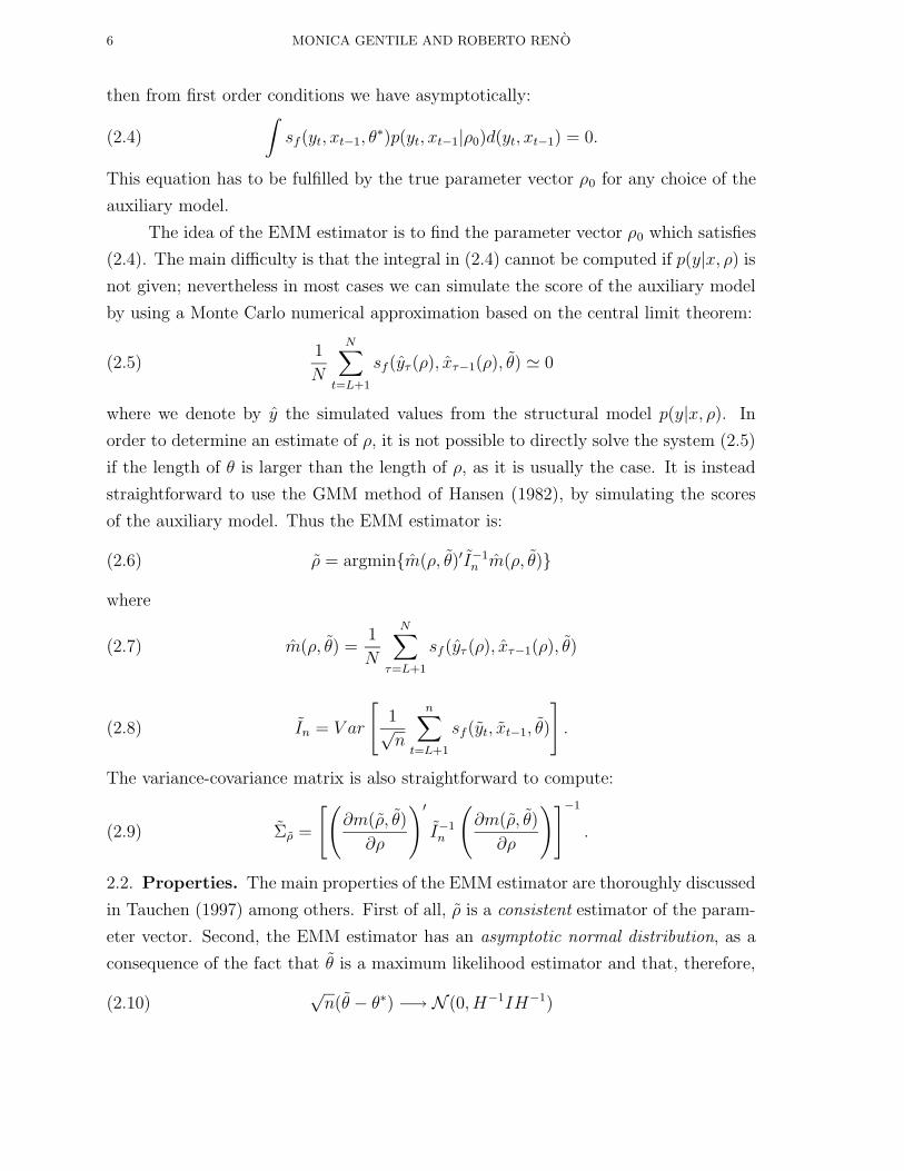
then from first order conditions we have asymptotically:
(2.4)
∫sf(yt, xt−1, θ
∗)p(yt, xt−1|ρ0)d(yt, xt−1) = 0.
This equation has to be fulfilled by the true parameter vector ρ0 for any choice of the
auxiliary model.
The idea of the EMM estimator is to find the parameter vector ρ0 which satisfies
(2.4). The main difficulty is that the integral in (2.4) cannot be computed if p(y|x, ρ) is
not given; nevertheless in most cases we can simulate the score of the auxiliary model
by using a Monte Carlo numerical approximation based on the central limit theorem:
(2.5)1
N
N∑
t=L+1
sf(yτ (ρ), xτ−1(ρ), θ) ' 0
where we denote by y the simulated values from the structural model p(y|x, ρ). In
order to determine an estimate of ρ, it is not possible to directly solve the system (2.5)
if the length of θ is larger than the length of ρ, as it is usually the case. It is instead
straightforward to use the GMM method of Hansen (1982), by simulating the scores
of the auxiliary model. Thus the EMM estimator is:
(2.6) ρ = argmin{m(ρ, θ)′I−1n m(ρ, θ)}
where
(2.7) m(ρ, θ) =1
N
N∑
τ=L+1
sf(yτ (ρ), xτ−1(ρ), θ)
(2.8) In = V ar
[1√n
n∑
t=L+1
sf(yt, xt−1, θ)
].
The variance-covariance matrix is also straightforward to compute:
(2.9) Σρ =
[(∂m(ρ, θ)
∂ρ
)′I−1n
(∂m(ρ, θ)
∂ρ
)]−1
.
2.2. Properties. The main properties of the EMM estimator are thoroughly discussed
in Tauchen (1997) among others. First of all, ρ is a consistent estimator of the param-
eter vector. Second, the EMM estimator has an asymptotic normal distribution, as a
consequence of the fact that θ is a maximum likelihood estimator and that, therefore,
(2.10)√n(θ − θ∗) −→ N (0, H−1IH−1)
WHICH MODEL FOR THE ITALIAN INTEREST RATES? 7
where H is the Hessian matrix of the log-likelihood function, while I is the Fisher
information matrix. Most important, if the auxiliary models nests the structural model,
EMM tends asymptotically to be as efficient as the maximum likelihood estimator
(Gallant and Long, 1995). Finally, it is useful to point out the fact that parameter
values that belong to instable or unacceptable regions of the parameter space cannot
minimize the chi-square function and consequently be the result of the estimation
process (Tauchen, 1997). This fact is illustrated in Andersen, Chung and Sorensen
(1999) by means of Monte Carlo experiments. It is suggested, instead, to check that θ
makes the auxiliary model stable.
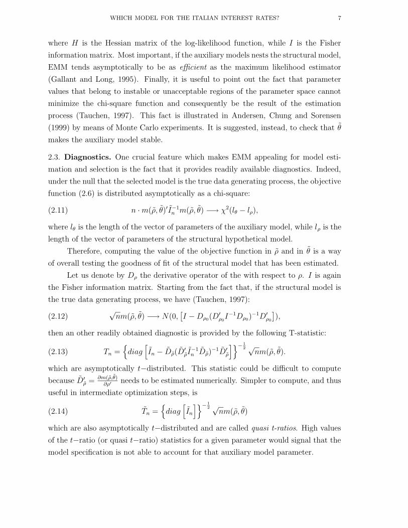
2.3. Diagnostics. One crucial feature which makes EMM appealing for model esti-
mation and selection is the fact that it provides readily available diagnostics. Indeed,
under the null that the selected model is the true data generating process, the objective
function (2.6) is distributed asymptotically as a chi-square:
(2.11) n ·m(ρ, θ)′I−1n m(ρ, θ) −→ χ2(lθ − lρ),
where lθ is the length of the vector of parameters of the auxiliary model, while lρ is the
length of the vector of parameters of the structural hypothetical model.
Therefore, computing the value of the objective function in ρ and in θ is a way
of overall testing the goodness of fit of the structural model that has been estimated.
Let us denote by Dρ the derivative operator of the with respect to ρ. I is again
the Fisher information matrix. Starting from the fact that, if the structural model is
the true data generating process, we have (Tauchen, 1997):
(2.12)√nm(ρ, θ) −→ N(0,
[I −Dρ0(D′ρ0
I−1Dρ0)−1D′ρ0
]),
then an other readily obtained diagnostic is provided by the following T-statistic:
(2.13) Tn ={diag
[In − Dρ(D
′ρI−1n Dρ)
−1D′ρ
]}− 12 √
nm(ρ, θ).
which are asymptotically t−distributed. This statistic could be difficult to compute
because D′ρ = ∂m(ρ,θ)∂ρ′ needs to be estimated numerically. Simpler to compute, and thus
useful in intermediate optimization steps, is
(2.14) Tn ={diag
[In
]}− 12 √
nm(ρ, θ)
which are also asymptotically t−distributed and are called quasi t-ratios. High values
of the t−ratio (or quasi t−ratio) statistics for a given parameter would signal that the
model specification is not able to account for that auxiliary model parameter.
8 MONICA GENTILE AND ROBERTO RENO
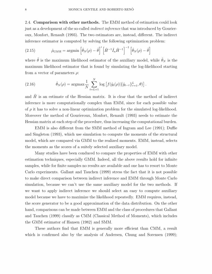
2.4. Comparison with other methods. The EMM method of estimation could look
just as a development of the so-called indirect inference that was introduced by Gourier-
oux, Monfort, Renault (1993). The two estimators are, instead, different. The indirect
inference estimator is computed by solving the following optimization problem:
(2.15) ρGMR = argmin[θN (ρ)− θ
]′ [H−1InH
−1]−1 [
θN (ρ)− θ]
where θ is the maximum likelihood estimator of the auxiliary model, while θN is the
maximum likelihood estimator that is found by simulating the log-likelihood starting
from a vector of parameters ρ:
(2.16) θN (ρ) = argmax1
N
N∑
t=L+1
log[f(yt(ρ)|{yt−τ}Lτ=1, θ)
].
and H is an estimate of the Hessian matrix. It is clear that the method of indirect
inference is more computationally complex than EMM, since for each possible value
of ρ it has to solve a non-linear optimization problem for the simulated log-likelihood.
Moreover the method of Gourieroux, Monfort, Renault (1993) needs to estimate the
Hessian matrix at each step of the procedure, thus increasing the computational burden.
EMM is also different from the SMM method of Ingram and Lee (1991); Duffie
and Singleton (1993), which use simulation to compute the moments of the structural
model, which are compared via GMM to the realized moments. EMM, instead, selects
the moments as the scores of a suitely selected auxiliary model.
Many studies have been conduced to compare the properties of EMM with other
estimation techniques, especially GMM. Indeed, all the above results hold for infinite
samples, while for finite samples no results are available and one has to resort to Monte
Carlo experiments. Gallant and Tauchen (1999) stress the fact that it is not possible
to make direct comparison between indirect inference and EMM through Monte Carlo
simulation, because we can’t use the same auxiliary model for the two methods. If
we want to apply indirect inference we should select an easy to compute auxiliary
model because we have to maximize the likelihood repeatedly. EMM requires, instead,
the score generator to be a good approximation of the data distribution. On the other
hand, comparisons can be made between EMM and the class of procedures that Gallant
and Tauchen (1999) classify as CMM (Classical Method of Moments), which includes
the GMM estimator of Hansen (1982) and SMM.
These authors find that EMM is generally more efficient than CMM, a result
which is confirmed also by the analysis of Andersen, Chung and Sorensen (1999);
WHICH MODEL FOR THE ITALIAN INTEREST RATES? 9
Chumacero (1997); Zhou (2001) also in small samples (n = 500), which is particularly
interesting for our application, in which n = 470.5 Moreover EMM improves the strong
over-rejection bias of GMM, while improving the rejection of misspecified models (Zhou,
2001). Ad hoc choice of moment conditions is probably the main reason of under-
performance of GMM and SMM. In the framework of EMM, the weighting matrix
is simpler to compute because the scores of a well fitted auxiliary model should be
approximately orthogonal. Andersen, Chung and Sorensen (1999) show that the t-
statistics are well-behaved even in small samples. Regarding efficiency, the theoretical
result of Gallant and Long (1995) is confirmed by Andersen, Chung and Sorensen
(1999): they evaluate EMM efficiency for samples of different size and they verify that
asymptotically (n = 4000) EMM efficiency is very close to that of maximum-likelihood.
Finally, Michaelides and Ng (2000) find, again by means of a Monte Carlo study in the
context of the theory of storage, that EMM over-performs both indirect inference and
SMM.
In general, we conclude that if the transition density is known maximum likeli-
hood or quasi-maximum likelihood should be preferred with respect to EMM. In all
other cases EMM provides a reasonable alternative.
3. The SNP algorithm
Selecting an auxiliary model that resumes the statistical properties of the ob-
served data is the central condition for a good performance of EMM procedure.
The choice of the auxiliary model (sometimes referred to as projection), in fact,
is tightly connected to the efficiency of EMM. The transition density used in the pro-
jection should closely approximate the distribution of the data. In the best case, if
the auxiliary model encompasses the structural one, EMM is as efficient as maximum
likelihood (Gallant and Long, 1995). Gallant and Tauchen (1989) proposed to use in
this first step of the procedure an expanding class of conditional densities that they
call SNP (Semi Non Parametric). The name SNP stems from the fact that, even if no
a-priori hypothesis is done, the projection represents a process of selection among a
family of parametric functions. To describe this class of densities we will let the process
5In Andersen, Chung and Sorensen (1999) it is shown that in small samples, the fit of an over-
identified auxiliary model, as those used later in this paper, can be problematic since it often results in
crashes or spurious fitting. They advocate, instead, close-to or perfectly identified moments. Since we
don’t experience such a problem, and this result is not confirmed by Chumacero (1997); Zhou (2001),
we guess that this effect strongly depends on the properties of the structural model.
10 MONICA GENTILE AND ROBERTO RENO
of interest {yt}∞t=−∞ depend on an innovation {zt}∞t=−∞ via:
(3.1) yt = Rx · zt + µx,
where y, z and µx, the location function, are vectors of size M while Rx, the scale
function, is an M ×M upper triangular matrix. The density of the innovation can be
approximated through an Hermite expansion:6
(3.3) h(z) =P 2(z)φ(z)∫P 2(s)φ(s)ds
,
where P is the Hermite polynomial of degree K and φ is a standard Normal multi-
variate density. The polynomial is squared to guarantee a positive density. To obtain
the density of the original process y we just need to apply the change of variables
transformation rule:
(3.4) f(yt|xt−1, θ) =P 2[R−1
x (yt − µx)]φ[R−1x (yt − µx)]/|det(Rx)|∫
P (s)2φ(s)ds
where φ[R−1x (yt− µx)]/|det(Rx)| is a Normal multivariate density, of argument y, with
mean µx and variance-covariance matrix Σx = Rx·R′x, K is the degree of the polynomial
P, while xt−1 is the vector of the past values of y. The parameter vector of this density,
θ, is estimated via maximum likelihood7.
An important property of the Hermite expansion, which makes it a good way
to approximate the data distribution, is that it represents a class of densities which
encompasses a lot of important statistical models. More precisely, if we indicate with
HK the domain of all SNP densities, for any choice of R and µ, in which the degree
of the P polynomial is K, the closure of the union H = ∪∞K=1HK under a weighted
Sobolev norm contains the density p(y|x, ρ) (Gallant and Tauchen, 1998). Moreover
under conditions easy to be verified SNP defines a consistent (Gallant and Nychka,
1987) estimator of the structural transition density p(y|x, ρ).
6This approach has its origin in the previous studies of Phillips (1983) who defines a function, called
ERA (Extended Rational Approximant), which takes the form:
(3.2) hERA(z) =P 2(z)
Q2(z)φ(z|µ,Σ).
7More precisely, to avoid negative densities induced by the numerics, we fit
(3.5) fK(yt|xt−1, θ) ={P 2
K [R−1x (yt − µx)] + ε0}φ[R−1
x (yt − µx)]/|det(Rx)|∫P 2K(s)φ(s)ds+ ε0
,
after setting ε0 = 1 · 10−5.
WHICH MODEL FOR THE ITALIAN INTEREST RATES? 11
After modeling the distribution of the residuals, we specify Rx and µx to introduce
dependence in the data. In particular we model µx as:
(3.6) µxt−1 = ψ0 + ψ1yt−1 + . . .+ ψLµyt−Lµ = ψ0 + Ψxt−1,
where xt−1 is the vector of the Lµ lagged values of each y variable. The conditional
heterogeneity of the stochastic process can be represented in the Hermite expansion by
introducing a dependence on P coefficients from yt−1. Following Gallant and Tauchen
(1989), the transition density f becomes:
(3.7) f(yt|xt−1, θ) =
[∑Kz|α|=1 Aα(yt−1)R−1
x (yt − ψ1 −Ψxt−1)α]2
nM(yt|µx,Σx)
∫ [∑Kz|α|=1 Aα(yt−1)uα
]2
φ(u)du,
with
(3.8) Aα(yt−1) =Kx∑
|β|=0
Aαβyβt−1.
To achieve identification A00 is set equal to one. We introduce conditional heteroscedas-
ticity in the variance-covariance matrix Σx in the following way. Setting Rx as:
(3.9)vech(Rx) = p0 +
∑Lri=1 Pi|yt−Lr+i − µxt−1−Lr+i
|+∑Lg
i=1 diag(Gi)vech(Rxt−1−Lg+i).
where vech(R) is the vector obtained with all the upper triangular elements of R,
p0, Pi are vectors of length M(M + 1)/2, G(1) through G(Lg) are vectors of length
M(M + 1)/2, we obtain a model similar to the GARCH model of Bollerslev (1986)8.
In particular, if M is equal to one we can write
(3.11)Rx = τ1 +
∑Lri=1 τa(i)|yt−Lr+i − µxt−1−Lr+i
|+∑Lg
i=1 τg(i)Rxt−1−Lg+i.
We remark that the just defined SNP model is still easily estimated via maximum
likelihood.
8The absolute value in (3.9) is not differentiable and, for this reason, it is substituted with a
trigonometric approximation
(3.10) a(u) =
{(|100u| − π
2 + 1)/100 |100u| ≥ π2
(1− cos(100u))/100 |100u| < π2
12 MONICA GENTILE AND ROBERTO RENO
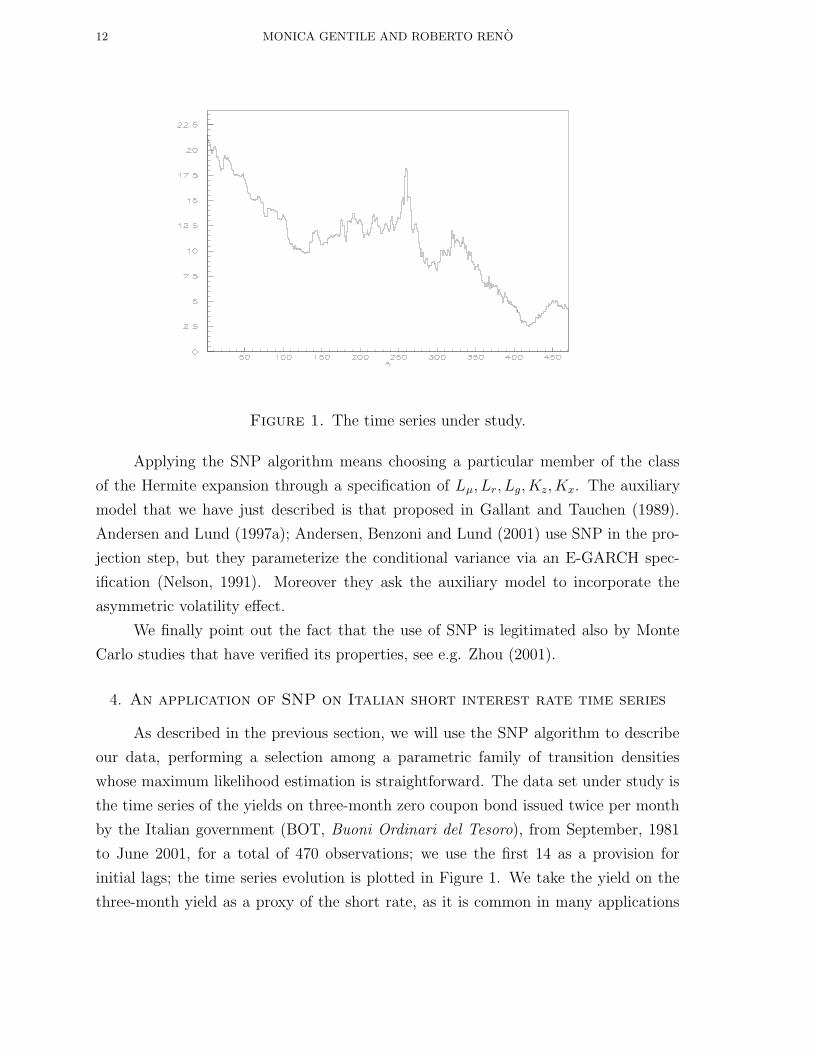
Figure 1. The time series under study.
Applying the SNP algorithm means choosing a particular member of the class
of the Hermite expansion through a specification of Lµ, Lr, Lg, Kz, Kx. The auxiliary
model that we have just described is that proposed in Gallant and Tauchen (1989).
Andersen and Lund (1997a); Andersen, Benzoni and Lund (2001) use SNP in the pro-
jection step, but they parameterize the conditional variance via an E-GARCH spec-
ification (Nelson, 1991). Moreover they ask the auxiliary model to incorporate the
asymmetric volatility effect.
We finally point out the fact that the use of SNP is legitimated also by Monte
Carlo studies that have verified its properties, see e.g. Zhou (2001).
4. An application of SNP on Italian short interest rate time series
As described in the previous section, we will use the SNP algorithm to describe
our data, performing a selection among a parametric family of transition densities
whose maximum likelihood estimation is straightforward. The data set under study is
the time series of the yields on three-month zero coupon bond issued twice per month
by the Italian government (BOT, Buoni Ordinari del Tesoro), from September, 1981
to June 2001, for a total of 470 observations; we use the first 14 as a provision for
initial lags; the time series evolution is plotted in Figure 1. We take the yield on the
three-month yield as a proxy of the short rate, as it is common in many applications
WHICH MODEL FOR THE ITALIAN INTEREST RATES? 13
(Gallant and Tauchen, 1998; Andersen and Lund, 1997a), see Chapman and Pearson
(2001) for a discussion on the economic relevance of this choice. As it can be seen in
Figure 1, the time series under study is sharply decreasing during the period at our
disposal9
The choice of the SNP model, as described in Section 3, is done via the choice of
the parameters Lµ, Lg, Lr, Kz, Kx that define an AR(Lµ)−SNP −GARCH(Lr, Lg)−P (Kz, Kx) model. Let us recall, in particular, that Kz is the degree of the rational
polynomial P in (3.3), while Kx is the maximum degree of each polynomial coefficient
Aα(yt−1) in (3.8). Several combinations of these parameters have been estimated10.
The goodness of the fit of a given model cannot be given simply by the maximum
likelihood:
(4.1) sn(θ) = − 1
n
n∑
t=(L+1)
log[f(yt|{yt−τ}Lτ=1, θ)],
since increasing the number of parameters always improves the value of the log-likelihood.
In order to introduce a penalty for over-parameterization, the usual technique is to con-
sider the Schwarz-Bayes, Akaike, Hannan and Quinn information criteria, defined as:
(4.2)
BIC = sn(θ) + 12(pθ/n) log(n)
AIC = sn(θ) + pθ/n
HQC = sn(θ) + (pθ/n) log[log(n)]
where pθ is the dimension of the parameter vector θ. The auxiliary density is chosen
after considering the information criteria. Generally, it is not guaranteed that these
different criteria provide the same indication.
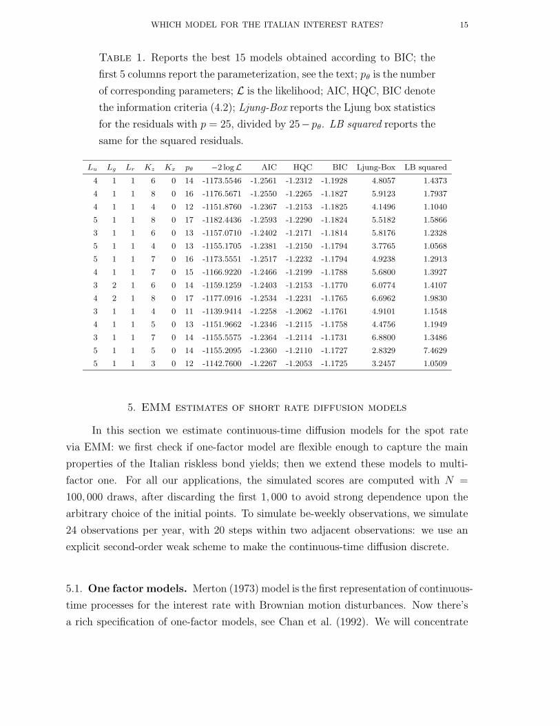
Table 1 summarizes the results for the best 15 models according to the most
popular BIC. In our case, the BIC criterion points towards 41160, while its second
choice is 41180 and its third choice is 41140. HQC would select again 41160, then
51180 and 41180. Finally, AIC would select 51180 as the first choice, and 41160, 41180
as the second and third choice. The tendency of AIC to select over-fitted auxiliary
9On the basis of the result of the Augmented Dickey Fuller test, we cannot reject the null hypothesis
of non stationarity at 95% confidence level (the test value is −2.2231, while the correspondent critical
value is −3.41). Nevertheless, in what follows, we will assume that our data are a sub-sample of a
stationary time series; for a colorful argument supporting this assumption see Cochrane (2001), p.
199.10Instead of using a branching tree, which could lead to miss some possible combinations, we
preferred to estimate all the possible combinations, with 0 ≤ Lµ ≤ 5, 0 ≤ Lr, Lg ≤ 2, 1 ≤ Kz ≤ 8, 0 ≤Kx ≤ 1
14 MONICA GENTILE AND ROBERTO RENO
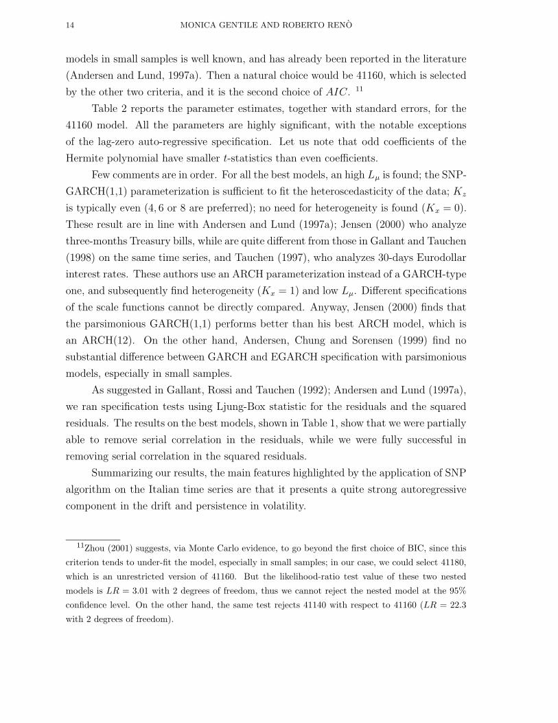
models in small samples is well known, and has already been reported in the literature
(Andersen and Lund, 1997a). Then a natural choice would be 41160, which is selected
by the other two criteria, and it is the second choice of AIC. 11
Table 2 reports the parameter estimates, together with standard errors, for the
41160 model. All the parameters are highly significant, with the notable exceptions
of the lag-zero auto-regressive specification. Let us note that odd coefficients of the
Hermite polynomial have smaller t-statistics than even coefficients.
Few comments are in order. For all the best models, an high Lµ is found; the SNP-
GARCH(1,1) parameterization is sufficient to fit the heteroscedasticity of the data; Kz
is typically even (4, 6 or 8 are preferred); no need for heterogeneity is found (Kx = 0).
These result are in line with Andersen and Lund (1997a); Jensen (2000) who analyze
three-months Treasury bills, while are quite different from those in Gallant and Tauchen
(1998) on the same time series, and Tauchen (1997), who analyzes 30-days Eurodollar
interest rates. These authors use an ARCH parameterization instead of a GARCH-type
one, and subsequently find heterogeneity (Kx = 1) and low Lµ. Different specifications
of the scale functions cannot be directly compared. Anyway, Jensen (2000) finds that
the parsimonious GARCH(1,1) performs better than his best ARCH model, which is
an ARCH(12). On the other hand, Andersen, Chung and Sorensen (1999) find no
substantial difference between GARCH and EGARCH specification with parsimonious
models, especially in small samples.
As suggested in Gallant, Rossi and Tauchen (1992); Andersen and Lund (1997a),
we ran specification tests using Ljung-Box statistic for the residuals and the squared
residuals. The results on the best models, shown in Table 1, show that we were partially
able to remove serial correlation in the residuals, while we were fully successful in
removing serial correlation in the squared residuals.
Summarizing our results, the main features highlighted by the application of SNP
algorithm on the Italian time series are that it presents a quite strong autoregressive
component in the drift and persistence in volatility.
11Zhou (2001) suggests, via Monte Carlo evidence, to go beyond the first choice of BIC, since this
criterion tends to under-fit the model, especially in small samples; in our case, we could select 41180,
which is an unrestricted version of 41160. But the likelihood-ratio test value of these two nested
models is LR = 3.01 with 2 degrees of freedom, thus we cannot reject the nested model at the 95%
confidence level. On the other hand, the same test rejects 41140 with respect to 41160 (LR = 22.3
with 2 degrees of freedom).
WHICH MODEL FOR THE ITALIAN INTEREST RATES? 15
Table 1. Reports the best 15 models obtained according to BIC; the
first 5 columns report the parameterization, see the text; pθ is the number
of corresponding parameters; L is the likelihood; AIC, HQC, BIC denote
the information criteria (4.2); Ljung-Box reports the Ljung box statistics
for the residuals with p = 25, divided by 25−pθ. LB squared reports the
same for the squared residuals.
Lu Lg Lr Kz Kx pθ −2 logL AIC HQC BIC Ljung-Box LB squared
4 1 1 6 0 14 -1173.5546 -1.2561 -1.2312 -1.1928 4.8057 1.4373
4 1 1 8 0 16 -1176.5671 -1.2550 -1.2265 -1.1827 5.9123 1.7937
4 1 1 4 0 12 -1151.8760 -1.2367 -1.2153 -1.1825 4.1496 1.1040
5 1 1 8 0 17 -1182.4436 -1.2593 -1.2290 -1.1824 5.5182 1.5866
3 1 1 6 0 13 -1157.0710 -1.2402 -1.2171 -1.1814 5.8176 1.2328
5 1 1 4 0 13 -1155.1705 -1.2381 -1.2150 -1.1794 3.7765 1.0568
5 1 1 7 0 16 -1173.5551 -1.2517 -1.2232 -1.1794 4.9238 1.2913
4 1 1 7 0 15 -1166.9220 -1.2466 -1.2199 -1.1788 5.6800 1.3927
3 2 1 6 0 14 -1159.1259 -1.2403 -1.2153 -1.1770 6.0774 1.4107
4 2 1 8 0 17 -1177.0916 -1.2534 -1.2231 -1.1765 6.6962 1.9830
3 1 1 4 0 11 -1139.9414 -1.2258 -1.2062 -1.1761 4.9101 1.1548
4 1 1 5 0 13 -1151.9662 -1.2346 -1.2115 -1.1758 4.4756 1.1949
3 1 1 7 0 14 -1155.5575 -1.2364 -1.2114 -1.1731 6.8800 1.3486
5 1 1 5 0 14 -1155.2095 -1.2360 -1.2110 -1.1727 2.8329 7.4629
5 1 1 3 0 12 -1142.7600 -1.2267 -1.2053 -1.1725 3.2457 1.0509
5. EMM estimates of short rate diffusion models
In this section we estimate continuous-time diffusion models for the spot rate
via EMM: we first check if one-factor model are flexible enough to capture the main
properties of the Italian riskless bond yields; then we extend these models to multi-
factor one. For all our applications, the simulated scores are computed with N =
100, 000 draws, after discarding the first 1, 000 to avoid strong dependence upon the
arbitrary choice of the initial points. To simulate be-weekly observations, we simulate
24 observations per year, with 20 steps within two adjacent observations: we use an
explicit second-order weak scheme to make the continuous-time diffusion discrete.
5.1. One factor models. Merton (1973) model is the first representation of continuous-
time processes for the interest rate with Brownian motion disturbances. Now there’s
a rich specification of one-factor models, see Chan et al. (1992). We will concentrate
16 MONICA GENTILE AND ROBERTO RENO
Table 2. Reports the fit of the AR(4)−SNP−GARCH(1, 1)−P (6, 0)
SNP model selected as a statistical description of the data. The param-
eters value are obtained via Maximum Likelihood. Standard errors are
computed via OPG.
Parameter Estimate Standard Error t-statistic
A10 -0.18400 0.09345 -1.969
A20 -0.32189 0.06035 -5.334
A30 0.08086 0.03511 2.303
A40 0.07415 0.01722 4.307
A50 -0.00722 0.00344 -2.099
A60 -0.00406 0.00124 -3.284
ψ0 -0.00045 0.00577 -0.079
ψ4 0.15400 0.04203 3.664
ψ3 -0.37898 0.05480 -6.916
ψ2 0.17221 0.06745 2.553
ψ1 1.04785 0.04870 21.517
τ1 0.01423 0.00335 4.254
τa 0.36425 0.07256 5.020
τg 0.60637 0.07302 8.304
on two very popular one-factor models: the Vasicek (1977) model:
(5.1) drt = α(γ − rt)dt+ σdWt.
and the CIR (Cox, Ingersoll and Ross, 1985a,b) model:
(5.2) drt = α(γ − rt)dt+ σ√rtdWt.
These models are both mean-reverting processes; the difference is in the diffusion term;
while the Vasicek model has Gaussian innovation, thus allowing for negative interest
rates, the CIR model has a non-central chi-square transition density, which prevents the
spot rate from becoming negative. Moreover the CIR model gives a mathematical rep-
resentation of the so-called ‘level effect’: indeed empirically it is observed that volatility
increases with the level of interest rates. This property cannot clearly be observed in
the Vasicek model. Both these models owe their popularity to the nice property that
closed-form expressions for the transition density and bond prices are readily available.

WHICH MODEL FOR THE ITALIAN INTEREST RATES? 17
In what follows, we will also deal with the Chan et al. (1992) specification of one-factor
models, the so-called constant elasticity of variance (CEV) model:
(5.3) drt = α(γ − rt)dt+ σtrξtdWt.
An important feature of the selected one-factor models is that they present a
linear drift, a property which is now a topic of debate in the literature: while both Ait-
Sahalia (1996); Stanton (1997) advocate a strong non-linearity in the drift, Chapman
and Pearson (2000) show by Monte Carlo that this finding could depend on the fact
that finite sample properties of the estimators adopted are not the same as asymptotic
properties. The however do not conclude in favor of a linear drift, but just show that
the rejection in Ait-Sahalia (1996); Stanton (1997) is doubtful. In a recent study, also
Christensen, Poulsen and Sorensen (2001) reject a non-linear drift. Anyway, we will
hold a linear drift throughout all our models, since in our opinion our data sample
is too small to detect non-linearities in the drift12. The results of the estimates for
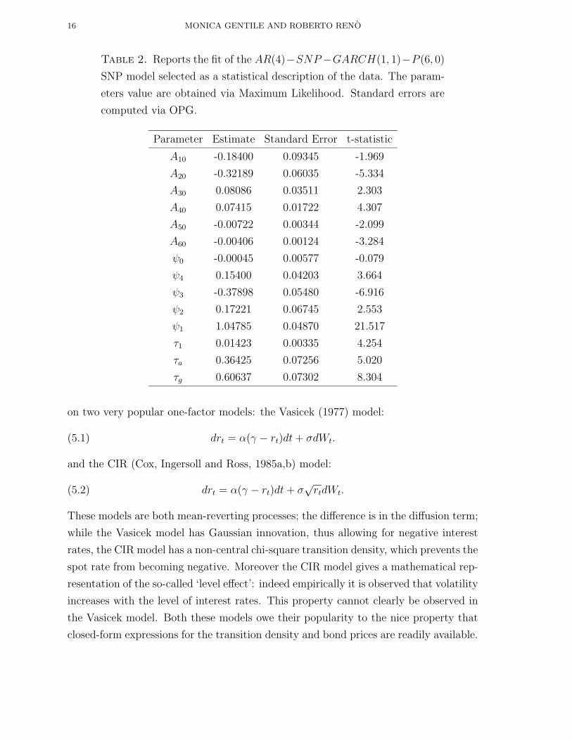
one-factor models are reported in Table 3. The CIR and Vasicek model has been
estimated through EMM several times on US short interest rate time series. In every
case (Tauchen, 1997; Andersen and Lund, 1997a; Gallant and Tauchen, 1998), they
have been firmly rejected. We confirm this result on the Italian time series, also if the
rejection is not so sharp: the χ2 for CIR is nearly 37, which is low when compared
with typical three-digits numbers obtained in similar studies: this is a consequence
of the smallness of our data sample. Anyway, both the one-factor model considered
are rejected. The long-run mean is estimated to be around 6-7%, while the mean-
reversion parameter is around 0.1: they are bot quite low, but it’s not surprising after
looking at the time series under study, which displays very slow mean reversion and
a decreasing shape. In order to assess the reliability of these results, we estimated
the CIR model via a linear regression, after discretizing the continuos-time model to
the first order, and via maximum likelihood, using the inversion of the characteristic
function suggested in Singleton (2001). Moreover, we compared our results to those
obtained by Barone, Cuoco and Zautzik (1991), who analyzed Italian bonds of different
maturities in the period 1984-1990, obtaining CIR estimates cross-sectionally. Table 4
shows the comparison: the estimates of the three parameters are reasonably the same
12Since non-linearities in the drift would be detected by rare extremely high or extremely low events,
Jones (2001) concludes that non-linearities cannot be detected even with the longest time series at
our disposal, the 5000 observations long T-bill daily time series. This issue, anyway, is yet an open
one.
18 MONICA GENTILE AND ROBERTO RENO
Table 3. One-factor model estimates.
Vasicek model
χ2(11) 37.511
Parameter Estimate 95% confidence interval
α 0.032 (0.019, 0.084)
γ 6.22 (3.28,8.34)
σ 1.15 (1.03, 1.29)
CIR model
χ2(11) 37.766
Parameter Estimate 95% confidence interval
α 0.1079 (0.1076, 0.1080)
γ 7.48 (7.47, 7.52)
σ 0.439 (0.438, 0.440)
CEV model
χ2(10) 36.237
Parameter Estimate 95% confidence interval
α 0.107 (0.103, 0.111)
γ 7.41 (7.30, 7.49)
σ 0.448 (0.438, 0.456)
ξ 0.493 (0.489, 0.505)
across different approaches; only the long-run mean estimated by Barone, Cuoco and
Zautzik (1991) is considerably higher, but only because they analized interest rates in a
period in which the interest rate level was higher. We then conclude that our estimates
are reliable, and they show that the considered one-factor model are not able to fit the
Italian data.
Extending to the CEV specification, no significant improvements in the chi-square
are observed. The parameter ξ has been estimated several times in the literature. In
WHICH MODEL FOR THE ITALIAN INTEREST RATES? 19
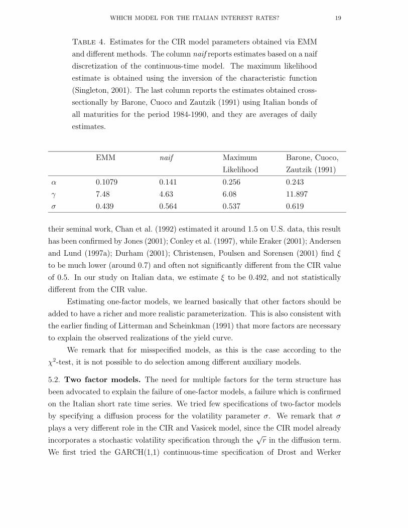
Table 4. Estimates for the CIR model parameters obtained via EMM
and different methods. The column naif reports estimates based on a naif
discretization of the continuous-time model. The maximum likelihood
estimate is obtained using the inversion of the characteristic function
(Singleton, 2001). The last column reports the estimates obtained cross-
sectionally by Barone, Cuoco and Zautzik (1991) using Italian bonds of
all maturities for the period 1984-1990, and they are averages of daily
estimates.
EMM naif Maximum Barone, Cuoco,
Likelihood Zautzik (1991)
α 0.1079 0.141 0.256 0.243
γ 7.48 4.63 6.08 11.897
σ 0.439 0.564 0.537 0.619
their seminal work, Chan et al. (1992) estimated it around 1.5 on U.S. data, this result
has been confirmed by Jones (2001); Conley et al. (1997), while Eraker (2001); Andersen
and Lund (1997a); Durham (2001); Christensen, Poulsen and Sorensen (2001) find ξ
to be much lower (around 0.7) and often not significantly different from the CIR value
of 0.5. In our study on Italian data, we estimate ξ to be 0.492, and not statistically
different from the CIR value.
Estimating one-factor models, we learned basically that other factors should be
added to have a richer and more realistic parameterization. This is also consistent with
the earlier finding of Litterman and Scheinkman (1991) that more factors are necessary
to explain the observed realizations of the yield curve.
We remark that for misspecified models, as this is the case according to the
χ2-test, it is not possible to do selection among different auxiliary models.
5.2. Two factor models. The need for multiple factors for the term structure has
been advocated to explain the failure of one-factor models, a failure which is confirmed
on the Italian short rate time series. We tried few specifications of two-factor models
by specifying a diffusion process for the volatility parameter σ. We remark that σ
plays a very different role in the CIR and Vasicek model, since the CIR model already
incorporates a stochastic volatility specification through the√r in the diffusion term.
We first tried the GARCH(1,1) continuous-time specification of Drost and Werker
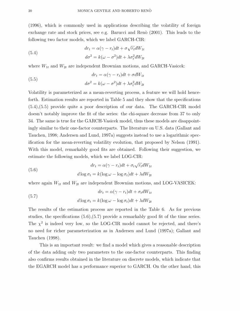
20 MONICA GENTILE AND ROBERTO RENO
(1996), which is commonly used in applications describing the volatility of foreign
exchange rate and stock prices, see e.g. Barucci and Reno (2001). This leads to the
following two factor models, which we label GARCH-CIR:
drt = α(γ − rt)dt+ σ√rtdW1t
dσ2 = k(ω − σ2)dt+ λσ2t dW2t
(5.4)
where W1t and W2t are independent Brownian motions, and GARCH-Vasicek:
drt = α(γ − rt)dt+ σdW1t
dσ2 = k(ω − σ2)dt+ λσ2t dW2t
(5.5)
Volatility is parameterized as a mean-reverting process, a feature we will hold hence-
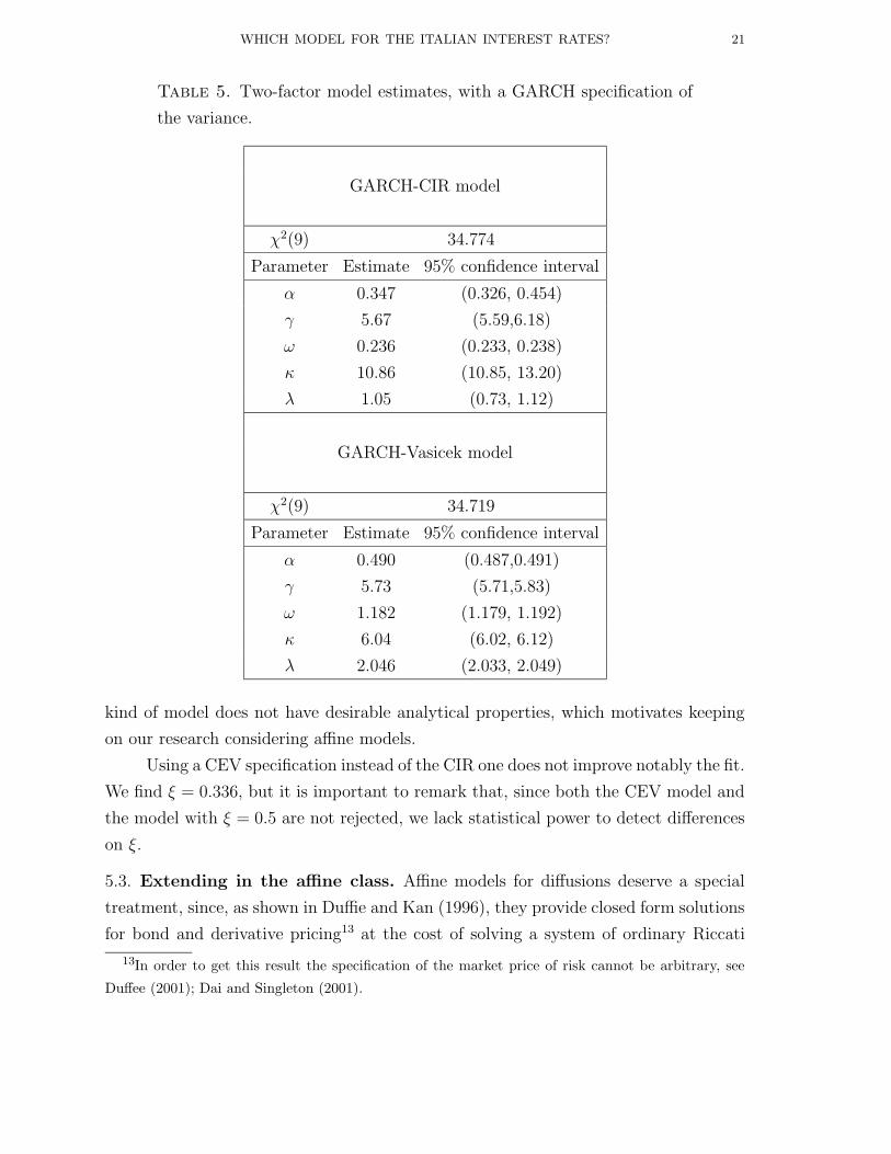
forth. Estimation results are reported in Table 5 and they show that the specifications
(5.4),(5.5) provide quite a poor description of our data. The GARCH-CIR model
doesn’t notably improve the fit of the series: the chi-square decrease from 37 to only
34. The same is true for the GARCH-Vasicek model, thus these models are disappoint-
ingly similar to their one-factor counterparts. The literature on U.S. data (Gallant and
Tauchen, 1998; Andersen and Lund, 1997a) suggests instead to use a logarithmic spec-
ification for the mean-reverting volatility evolution, that proposed by Nelson (1991).
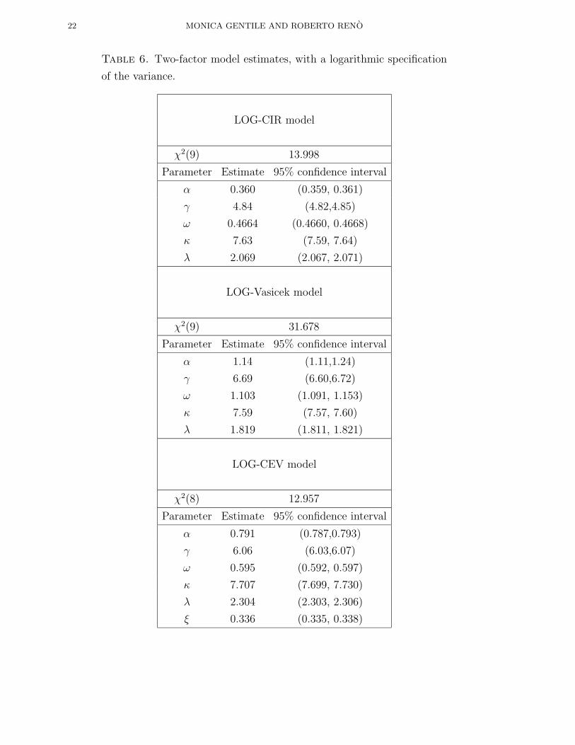
With this model, remarkably good fits are obtained. Following their suggestion, we
estimate the following models, which we label LOG-CIR:
drt = α(γ − rt)dt+ σt√rtdW1t
d log σt = k(logω − log σt)dt+ λdW2t
(5.6)
where again W1t and W2t are independent Brownian motions, and LOG-VASICEK:
drt = α(γ − rt)dt+ σtdW1t
d log σt = k(logω − log σt)dt+ λdW2t
(5.7)
The results of the estimation process are reported in the Table 6. As for previous
studies, the specifications (5.6),(5.7) provide a remarkably good fit of the time series.
The χ2 is indeed very low, so the LOG-CIR model cannot be rejected, and there’s
no need for richer parameterization as in Andersen and Lund (1997a); Gallant and
Tauchen (1998).
This is an important result: we find a model which gives a reasonable description
of the data adding only two parameters to the one-factor counterparts. This finding
also confirms results obtained in the literature on discrete models, which indicate that
the EGARCH model has a performance superior to GARCH. On the other hand, this
WHICH MODEL FOR THE ITALIAN INTEREST RATES? 21
Table 5. Two-factor model estimates, with a GARCH specification of
the variance.
GARCH-CIR model
χ2(9) 34.774
Parameter Estimate 95% confidence interval
α 0.347 (0.326, 0.454)
γ 5.67 (5.59,6.18)
ω 0.236 (0.233, 0.238)
κ 10.86 (10.85, 13.20)
λ 1.05 (0.73, 1.12)
GARCH-Vasicek model
χ2(9) 34.719
Parameter Estimate 95% confidence interval
α 0.490 (0.487,0.491)
γ 5.73 (5.71,5.83)
ω 1.182 (1.179, 1.192)
κ 6.04 (6.02, 6.12)
λ 2.046 (2.033, 2.049)
kind of model does not have desirable analytical properties, which motivates keeping
on our research considering affine models.
Using a CEV specification instead of the CIR one does not improve notably the fit.
We find ξ = 0.336, but it is important to remark that, since both the CEV model and
the model with ξ = 0.5 are not rejected, we lack statistical power to detect differences
on ξ.
5.3. Extending in the affine class. Affine models for diffusions deserve a special
treatment, since, as shown in Duffie and Kan (1996), they provide closed form solutions
for bond and derivative pricing13 at the cost of solving a system of ordinary Riccati
13In order to get this result the specification of the market price of risk cannot be arbitrary, see
Duffee (2001); Dai and Singleton (2001).
22 MONICA GENTILE AND ROBERTO RENO
Table 6. Two-factor model estimates, with a logarithmic specification
of the variance.
LOG-CIR model
χ2(9) 13.998
Parameter Estimate 95% confidence interval
α 0.360 (0.359, 0.361)
γ 4.84 (4.82,4.85)
ω 0.4664 (0.4660, 0.4668)
κ 7.63 (7.59, 7.64)
λ 2.069 (2.067, 2.071)
LOG-Vasicek model
χ2(9) 31.678
Parameter Estimate 95% confidence interval
α 1.14 (1.11,1.24)
γ 6.69 (6.60,6.72)
ω 1.103 (1.091, 1.153)
κ 7.59 (7.57, 7.60)
λ 1.819 (1.811, 1.821)
LOG-CEV model
χ2(8) 12.957
Parameter Estimate 95% confidence interval
α 0.791 (0.787,0.793)
γ 6.06 (6.03,6.07)
ω 0.595 (0.592, 0.597)
κ 7.707 (7.699, 7.730)
λ 2.304 (2.303, 2.306)
ξ 0.336 (0.335, 0.338)
WHICH MODEL FOR THE ITALIAN INTEREST RATES? 23
differential equations, which can be solved with very fast, accurate and easily available
algorithms, while different models need the solution of a partial differential equation,
much harder to solve, even numerically. It is worth to note that CIR and Vasicek
model are affine models, that’s why a closed form solution exists.
We start by experimenting all the possible two-factor affine model. As a second
factor we can choose the mean, resulting in the AFFINE-MEAN model:
(5.8)drt = α(γt − rt)dt+ σ
√rtdW1t
dγt = θ(ν − γt)dt+ η√γtdW2t,
or the volatility, getting the AFFINE-VOL model:
(5.9)drt = α(γ − rt)dt+
√σtdW1t
dσt = k(ω − σt)dt+ λ√σtdW2t
which can be extended to account for correlation among Brownian motions:
(5.10)drt = α(γ − rt)dt+
√σtdW1t + ρσrλ
√σtdW2t
dσt = k(ω − σt)dt+ λ√σtdW2t
Model (5.9) is the same as model (5.10) after setting ρσr = 0. Estimation results, shown
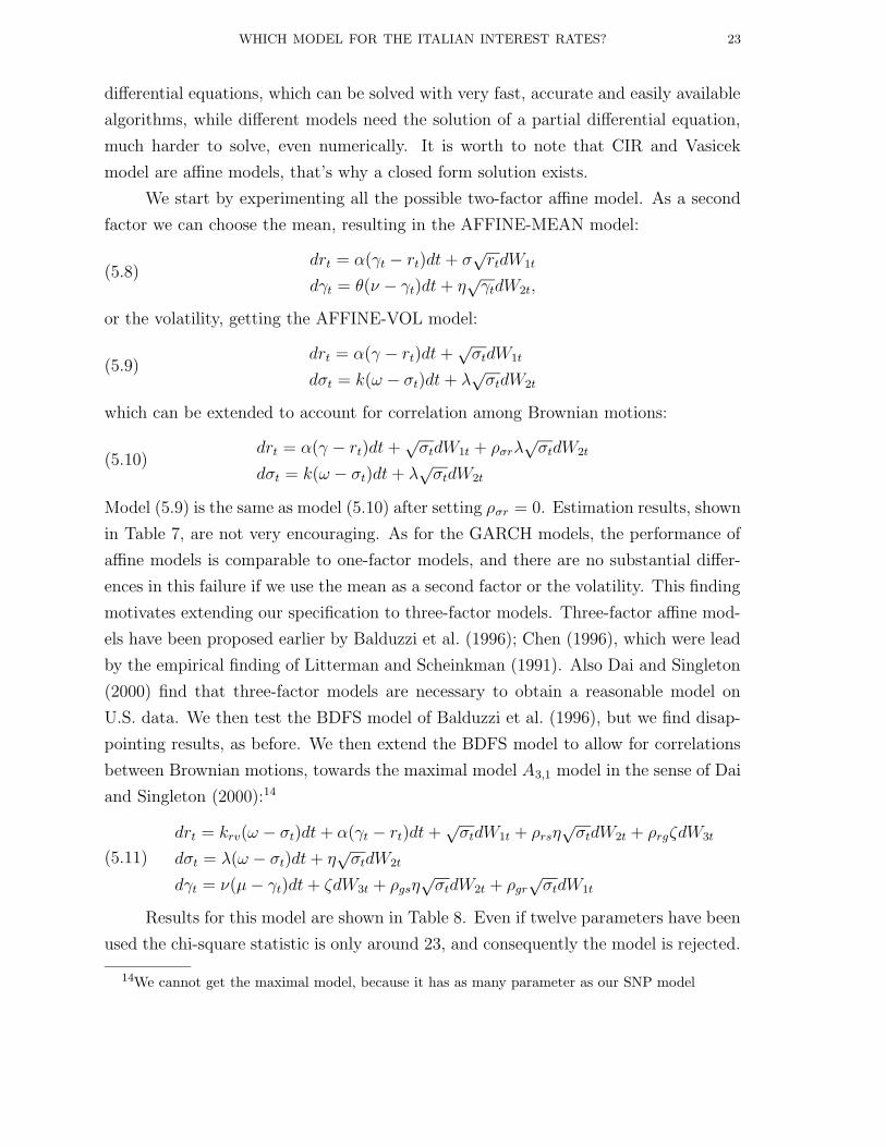
in Table 7, are not very encouraging. As for the GARCH models, the performance of
affine models is comparable to one-factor models, and there are no substantial differ-
ences in this failure if we use the mean as a second factor or the volatility. This finding
motivates extending our specification to three-factor models. Three-factor affine mod-
els have been proposed earlier by Balduzzi et al. (1996); Chen (1996), which were lead
by the empirical finding of Litterman and Scheinkman (1991). Also Dai and Singleton
(2000) find that three-factor models are necessary to obtain a reasonable model on
U.S. data. We then test the BDFS model of Balduzzi et al. (1996), but we find disap-
pointing results, as before. We then extend the BDFS model to allow for correlations
between Brownian motions, towards the maximal model A3,1 model in the sense of Dai
and Singleton (2000):14
(5.11)
drt = krv(ω − σt)dt+ α(γt − rt)dt+√σtdW1t + ρrsη
√σtdW2t + ρrgζdW3t
dσt = λ(ω − σt)dt+ η√σtdW2t
dγt = ν(µ− γt)dt+ ζdW3t + ρgsη√σtdW2t + ρgr
√σtdW1t
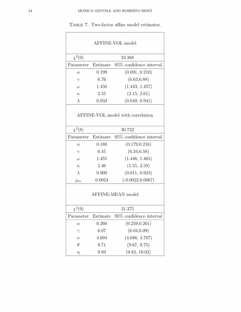
Results for this model are shown in Table 8. Even if twelve parameters have been
used the chi-square statistic is only around 23, and consequently the model is rejected.
14We cannot get the maximal model, because it has as many parameter as our SNP model
24 MONICA GENTILE AND ROBERTO RENO
Table 7. Two-factor affine model estimates.
AFFINE-VOL model
χ2(9) 33.388
Parameter Estimate 95% confidence interval
α 0.199 (0.091, 0.210)
γ 6.76 (6.63,6.88)
ω 1.450 (1.443, 1.457)
κ 2.55 (2.15, 2.61)
λ 0.933 (0.849, 0.941)
AFFINE-VOL model with correlation
χ2(8) 30.732
Parameter Estimate 95% confidence interval
α 0.180 (0.179,0.216)
γ 6.45 (6.34,6.58)
ω 1.455 (1.446, 1.465)
κ 2.46 (1.55, 2.59)
λ 0.909 (0.811, 0.923)
ρσr 0.0024 (-0.0022,0.0067)
AFFINE-MEAN model
χ2(9) 31.375
Parameter Estimate 95% confidence interval
α 0.260 (0.259,0.261)
γ 6.07 (6.04,6.09)
ν 4.694 (4.686, 4.707)
θ 9.71 (9.67, 9.75)
η 9.89 (9.82, 10.02)
WHICH MODEL FOR THE ITALIAN INTEREST RATES? 25
Table 8. Three-factor BDFS model estimates.
Extended BDFS model
χ2(6) 23.467
Parameter Estimate 95% confidence interval
krv 4.26 (-7.28, 10.39)
ω 0.44 (0.42,0.49)
α 3.95 (1.86,5.17)
ν 3.35 (3.20,3.54)
µ 4.13 (4.01,4.25)
λ 1.04 (0.70,1.12)
ρrg 0.49 (0.31, 0.66)
ζ 1.19 (0.83, 1.74)
ρrs 1.52 (1.45, 1.57)
η 0.6964 (0.6963, 0.6965)
ρgs -2.37 (-7.09, -0.67)
ρgr -3.27 (-5.55, -2.91)
We conclude that, differently with the findings of Dai and Singleton (2000) on
U.S. data, affine models, up to three-factors, are not able to provide a completely
satisfactory statistical description of the Italian data.
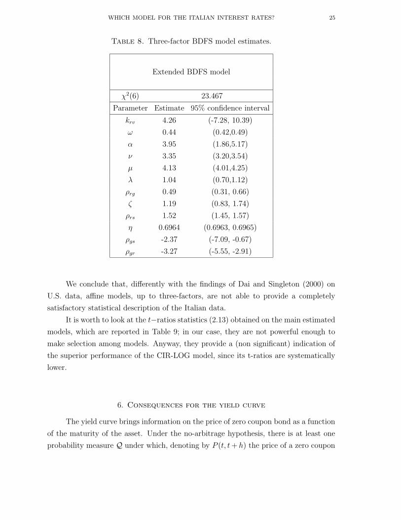
It is worth to look at the t−ratios statistics (2.13) obtained on the main estimated
models, which are reported in Table 9; in our case, they are not powerful enough to
make selection among models. Anyway, they provide a (non significant) indication of
the superior performance of the CIR-LOG model, since its t-ratios are systematically
lower.
6. Consequences for the yield curve
The yield curve brings information on the price of zero coupon bond as a function
of the maturity of the asset. Under the no-arbitrage hypothesis, there is at least one
probability measure Q under which, denoting by P (t, t+ h) the price of a zero coupon
26 MONICA GENTILE AND ROBERTO RENO
Table 9. T-ratios for the main estimated models.
Parameter CIR AFFINE-VOL CIR-LOG Extended BDFS
A10 -1.031 -1.521 -0.172 0.619
A20 0.966 0.456 0.474 3.079
A30 0.245 0.744 0.227 3.121
A40 1.251 0.713 0.384 1.707
A50 0.103 0.430 -0.191 1.657
A60 0.561 0.055 0.191 -0.03
ψ0 -0.357 -0.698 -0.267 -0.672
ψ4 1.580 1.290 0.267 0.990
ψ3 1.557 1.280 0.215 0.995
ψ2 1.425 1.129 0.138 1.080
ψ1 1.530 1.224 0.177 1.104
τ1 0.435 -0.392 0.020 -0.221
τa 0.704 0.237 0.750 0.869
τg 0.429 -0.131 0.444 -0.211
bond issued in t with maturity in t+ h:
(6.1) P (t, t+ h) = EQt
[e−
∫ t+ht rsds
],
where EQt denotes conditional expectation with respect to Q. Then the yield curve is
given by:
(6.2) f(t, h) =logP (t, t+ h)
h.
In this Section, we check if the logarithmic specification (5.6), which we found
to be the best among all the diffusion models tested, can account for the observed
yield curves. Indeed, one great operational problem of one-factor models like CIR and
Vasicek, is that they are not flexible enough to account for the empirical properties of
the observed yield curves; for example, they cannot reproduce the inverse hump which
is sometimes observed around the maturity of one year. This problem has also been
raised and studied by Andersen and Lund (1997b).
For the model (5.6), the yield curve can only be computed via Monte Carlo
simulations, since no closed formulas are available. Since in (6.1) the expected value
is computed under the risk neutral probability, it is necessary to modify the drift by
WHICH MODEL FOR THE ITALIAN INTEREST RATES? 27
introducing the market price of risk, obtaining the modified short-rate diffusion:
(6.3) drt = [µt(rt)− λrσt(rt)]dt+ σt(rt)dWt.
We have a bivariate diffusion, so we need two market prices of risk; following the
example of Andersen and Lund (1997b) we specify the market price of risk via λ1 =
−0.3√rt, λ2 = 0, i.e. we assume that the volatility risk is not priced and we choose
a negative λ1 to offset the convexity bias. It is worth to remark that our purpose
is merely illustrative, and we are not going to calibrate the market prices of risk on
observed yield curves, neither to test if the volatility risk is priced. The market price
of risk λ1 introduces the volatility into the drift of the short rate, thus allowing richer
dynamics.
Let us remark that the functional form of the yield curve at time t will depend
on the values of r(t) and σ(t). Given r and σ at time t, and the market prices of risk,
the yield curve (6.2) is completely specified, as a function of h, by the model.
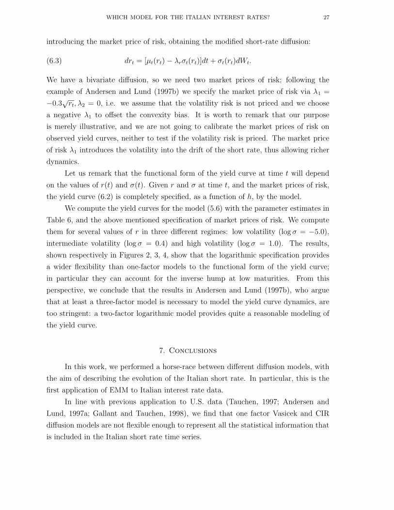
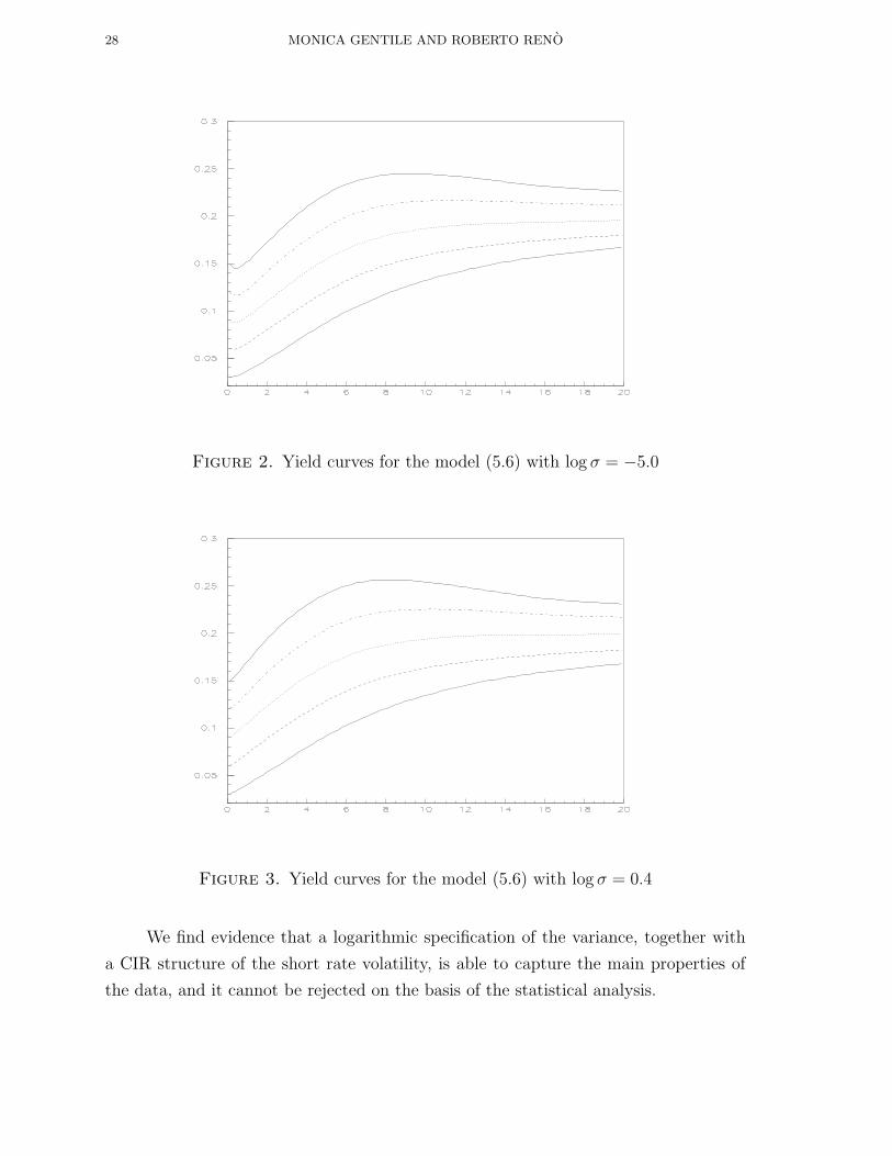
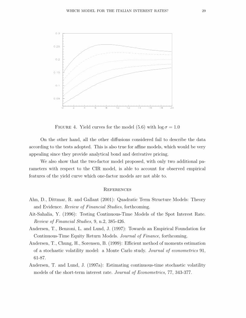
We compute the yield curves for the model (5.6) with the parameter estimates in
Table 6, and the above mentioned specification of market prices of risk. We compute
them for several values of r in three different regimes: low volatility (log σ = −5.0),
intermediate volatility (log σ = 0.4) and high volatility (log σ = 1.0). The results,
shown respectively in Figures 2, 3, 4, show that the logarithmic specification provides
a wider flexibility than one-factor models to the functional form of the yield curve;
in particular they can account for the inverse hump at low maturities. From this
perspective, we conclude that the results in Andersen and Lund (1997b), who argue
that at least a three-factor model is necessary to model the yield curve dynamics, are
too stringent: a two-factor logarithmic model provides quite a reasonable modeling of
the yield curve.
7. Conclusions
In this work, we performed a horse-race between different diffusion models, with
the aim of describing the evolution of the Italian short rate. In particular, this is the
first application of EMM to Italian interest rate data.
In line with previous application to U.S. data (Tauchen, 1997; Andersen and
Lund, 1997a; Gallant and Tauchen, 1998), we find that one factor Vasicek and CIR
diffusion models are not flexible enough to represent all the statistical information that
is included in the Italian short rate time series.
28 MONICA GENTILE AND ROBERTO RENO
Figure 2. Yield curves for the model (5.6) with log σ = −5.0
Figure 3. Yield curves for the model (5.6) with log σ = 0.4
We find evidence that a logarithmic specification of the variance, together with
a CIR structure of the short rate volatility, is able to capture the main properties of
the data, and it cannot be rejected on the basis of the statistical analysis.
WHICH MODEL FOR THE ITALIAN INTEREST RATES? 29
Figure 4. Yield curves for the model (5.6) with log σ = 1.0
On the other hand, all the other diffusions considered fail to describe the data
according to the tests adopted. This is also true for affine models, which would be very
appealing since they provide analytical bond and derivative pricing.
We also show that the two-factor model proposed, with only two additional pa-
rameters with respect to the CIR model, is able to account for observed empirical
features of the yield curve which one-factor models are not able to.
References
Ahn, D., Dittmar, R. and Gallant (2001): Quadratic Term Structure Models: Theory
and Evidence. Review of Financial Studies, forthcoming.
Ait-Sahalia, Y. (1996): Testing Continuous-Time Models of the Spot Interest Rate.
Review of Financial Studies, 9, n.2, 385-426.
Andersen, T., Benzoni, L. and Lund, J. (1997): Towards an Empirical Foundation for
Continuous-Time Equity Return Models. Journal of Finance, forthcoming.
Andersen, T., Chung, H., Sorensen, B. (1999): Efficient method of moments estimation
of a stochastic volatility model: a Monte Carlo study. Journal of econometrics 91,
61-87.
Andersen, T. and Lund, J. (1997a): Estimating continuous-time stochastic volatility
models of the short-term interest rate. Journal of Econometrics, 77, 343-377.
30 MONICA GENTILE AND ROBERTO RENO
Andersen, T. and Lund, J. (1997b): Stochastic volatility and mean drift in the short
rate diffusion: sources of steepness, level and curvature in the yield curve. North-
western University, Kellogg Graduate School of Management, Working Paper N.214.
Balduzzi, P., Das, S., Foresi, S. and Sundaram, R. (1996): A simple approach to three
factor affine term structure models. Journal of Fixed Income, 6, 43-53.
Balduzzi, P., Elton, E. and Green, T.C. (2001): Economic News and Bond Prices:
Evidence from the U.S. Treasury Market. Journal of Financial and Quantitative
Analysis, 36, No. 4, December 2001.
Bansal, R., Gallant, R., Hussey, R. and Tauchen, G. (1995): Nonparametric estimation
of structural models for high-frequency currency market data. Journal of Economet-
rics, 66, 251-287.
Bansal, R. and Zhou, H. (2001): Term Structure of Interest Rates with Regime Shifts.
Journal of Finance, forthcoming.
Barone, E., Cuoco, D. and Zautzik, E. (1991): Term structure estimation using the
Cox, Ingersoll and Ross model: the case of Italian Treasury bonds. Journal of Fixed
Income, 1, 13, 87-95.
Barucci, E. and Reno, R. (2001): On measuring volatility and the GARCH forecasting
performance. Forthcoming Journal of International Financial Markets, Institutions
and Money.
Benzoni, L. (1999): Pricing Options under Stochastic Volatility: An Econometric Anal-
ysis. Manuscript.
Bollerslev, T. (1986): Generalized autoregressive conditional heteroskedasticity. Jour-
nal of Econometrics 31, 307-327.
Brandt, M.W. and Santa-Clara, P. (2001): Simulated Likelihood Estimation of Dif-
fusions with an Application to Exchange Rate Dynamics in Incomplete Markets.
Journal of Financial Economics, forthcoming.
Chapman, D. and Pearson, N. (2000): Is the Short Rate Drift Actually Nonlinear?
Journal of Finance, 55(1), 355-388.
Chapman, D. and Pearson, N. (2001): Recent Advances in Estimating Term-Structure
Models. Financial Analysts Journal, 57(4), pages 77-95.
Chan, K.C., Karolyi, G.A., Longstaff, F.A. F.A., and Sanders, A.B., (1992): An em-
pirical comparison of alternative models of the short-term interest rate. Journal of
Finance, 47, 1209-1227.
WHICH MODEL FOR THE ITALIAN INTEREST RATES? 31
Chen, L. (1996): Stochastic Mean and Stochastic Volatility - a Three-Factor Model of
the Term Structure of Interest Rates and its Application in Derivatives Pricing and
Risk Management. Financial Markets, Institutions and Instruments, 5, No. 1.
Chernov, M. and Ghysels, E. (2000): A study towards a unified approach to the joint
estimation of objective and risk neutral measures for the purpose of options valuation.
Journal of Financial Economics, 56, 407-458.
Chernov, M., Gallant, R., Ghysels, E. and Tauchen G. (2001): Alternative Models for
Stock Price Dynamics. Manuscript.
Christensen, Poulsen and Sorensen (2001): Optimal inference in diffusion models of
the short rate of interest. CAF Working Paper Series No. 102.
Chumacero, R. (1997): Finite Sample Properties of the Efficient Method of Moments.
Studies in Nonlinear Dynamics and Econometrics, 74, 77-118.
Chung, C.S. and Tauchen, G. (2001): Testing Target Zone Models Using Efficient
Method of Moments. Forthcoming, Journal of Business and Economic Statistics.
Cochrane, J. (2001): Asset pricing. Princeton University Press.
Conley, T., Hansen, L.P., Luttmer, E. and Scheinkman, J. (1997): Short-Term Interest
Rates as Subordinated Diffusions. Review of Financial Studies, 10(3), 525-577.
Cox, J. C., Ingersoll, J. E., Ross, S. A. (1985a): An inter-temporal general equilibrium
model of asset prices. Econometrica, 53, 363-384
Cox, J. C., Ingersoll, J. E., Ross, S. A. (1985b): A theory of the term structure of
interest rates. Econometrica, 53, 385-406
Craine, R., Lochstoer, L. and Syrtveit, K. (2000): Estimation of a Stochastic-Volatility
Jump-Diffusion Model. Manuscript.
Dai, Q. and Singleton, K. (2000): Specification Analysis of Affine Term-Structure
Models. Journal of Finance, 55(5), 1943-1978.
Dai, Q. and Singleton, K. (2001): Expectation Puzzles, Time-Varying Risk Premia,
and Dynamic Models of the Term Structure. Manuscript.
Drost, F. and Werker, B., 1996: Closing the GARCH Gap: Continuous Time GARCH
Models. Journal of Econometrics, 74: 31-57.
Duffee, G. (2001): Term Premia and Interest Rate Forecasts in Affine Models. Journal
of Finance, forthcoming.
Duffie, D., Kan, R. (1996): A yield factor model of interest rates. Mathematical Fi-
nance, 6, 379-406
32 MONICA GENTILE AND ROBERTO RENO
Duffie, D., Singleton, K.J., 1993: Simulated moments estimation of Markov of asset
prices. Econometrica, 61, 929-952.
Durham, G. (2001): Likelihood-Based Specification Analysis of Continuous-Time Mod-
els of the Short-Term Interest Rate. Manuscript, University of Iowa.
Elerian, O., Chib, S. and Shephard, N. (2001): Likelihood inference for discretely
observed non-linear diffusions. Econometrica, forthcoming.
Eraker, B. (2001): MCMC Analysis of Diffusion Models With Application to Finance.
Journal of Business and Economic Statistics, 19(2), 177-191.
Fenton, V. and Gallant, R. (1996): Convergence rates of SNP density estimators.
Econometrica, 64, n.3, 719-727.
Fleming, M.J. and E.M. Remolona (1999): Price Formation and Liquidity in the U.S.
Treasury Market: The Response to Public Information. Journal of Finance, 54, 5,
1901-15.
Gallant, A.R. and Nychka, D.W.(1987): Semi-nonparametric maximum likelihood es-
timation. Econometrica, 55, 363-90.
Gallant, A.R. and Long, J.R.(1995): Estimating stochastic differential equations effi-
ciently by minimum chi-square. Biometrika.
Gallant, R., Hsu, C.T. and Tauchen, G. (1999): Using Daily Range Data to Cali-
brate Volatility Diffusions and Extract the Forward Integrated Variance. Review of
Economic and Statistics, 81, 617-631.
Gallant,A.R., Rossi, P.E. and Tauchen, G. (1992): Stock Prices and Volume. The
Review of Financial Studies, v.5, n.2.
Gallant, R. and Tauchen, G. (1989): Seminonparametric Estimation of Conditionally
Constrained Heterogeneous Processes: Asset pricing Applications. Econometrica, 57,
1091-1121.
Gallant, R. and Tauchen, G. (1996): Which moments to match? Econometric Theory,
657-681.
Gallant, R. and Tauchen, G. (1998): Reprojecting partially observed systems with
application to interest rate diffusions. Journal of American Statistical Association,
93, No.441.
Gallant, R., Tauchen, G.,(1999): The relative efficiency of method of moments estima-
tors. Journal of Econometrics, 92, 149-172.
Gallant, R. and Tauchen,G. (2001a): SNP: A program for Nonparametric Time Series
Analysis, Version 8.8, User’s Guide.
WHICH MODEL FOR THE ITALIAN INTEREST RATES? 33
Gallant, R. and Tauchen,G. (2001b): EMM. A Program for Efficient Method of Mo-
ments Estimation, Version 1.6, User’s Guide.
Gallant, R. and Tauchen,G. (2001c): Efficient Method of Moments. Manuscript.
Gourieroux, C., Monfort, A., and Renault, E. (1993): Indirect Inference. Journal of
Applied Econometrics, 8: S85-S118.
Hansen, L.P. and Scheinkman, J. (1982): Large sample properties of generalized
method of moments estimators. Econometrica, 63, 767-804.
Ingram, B.F., Lee, B.S., 1991: Simulation estimation of time series models. Journal of
Econometrics, 47, 197-250.
Jacquier, E., Polson, N. and Rossi, P. (1994): Bayesian Analysis of Stochastic Volatility
Models. Journal of Business and Economic Statistics, 12, 371-389.
Jensen, M.B. (2000): Efficient Method of Moments Estimation of the Longstaff and
Schwartz Interest Rate Model. CAF Working paper.
Jiang, G. and van der Sluis, P. (1999): Pricing Stock Options under Stochastic Volatil-
ity and Interest Rates with Efficient Method of Moments Estimation. Manuscript,
University of Groningen and Tilburg University.
Jones, C. (2001): Nonlinear Mean Reversion in the Short-Term Interest Rate. Manu-
script.
Litterman, R. and Sheinkman, J. (1991): Common Factors Affecting Bond Returns.
Journal of Fixed Income, 1, 54-61.
Mari, C. and Reno, R. (2001). Credit Risk Analysis of Mortgage Loans: an Application
to the Italian Market. Quaderni del Dipartimento di Economia Politica, Universita
di Siena.
Merton, R.C., (1973): Theory of rational option pricing. Bell Journal of Economics
and Mangement Science 4, 141-183.
Michaelides, A. and Ng, S. (2000): Estimating the rational expectations model of spec-
ulative storage: A Monte Carlo comparison of tree simulation estimators. Journal of
Econometrics, 96. 231-266.
Nelson, D.B., 1991, Conditional heteroskedasticity in asset returns: A new approach.
Econometrica 59, 347-370.
Pearson, N. and Sun, T-S. (1994): Exploiting the conditional density in estimating
the term structure: An application to the Cox, Ingersoll and Ross model. Journal of
Finance, 49, 1279-1304.
34 MONICA GENTILE AND ROBERTO RENO
Pedersen, A.R. (1995): A new approach to maximum kileihood estimation for stochatic
differential equations based on discrete observations. Scandinavian Journal of Sta-
tistics, 22, 55-71.
Phillips P. (1983): ERA’s: A New Approach to Small Sample Theory. Econometrica,
51, 1505-1527.
Piazzesi, M. (2001): An econometric Model of the Yield Curve with Macroeconomic
Jump Effects. NBER Working Paper.
Sundaresan, S. (2000): Continuous-Time Methods in Finance: A Review and an As-
sessment. Journal of Finance, 55, n.4, 1569-1622.
Singleton, K. (2001): Estimation of affine asset pricing models using the empirical
characteristic function. Journal of Econometrics, forthcoming.
Stanton, R. (1997): A Nonparametric Model of Term Structure Dynamics and the
Market Price of Interest Rate Risk. Journal of Finance, 52(5), 1973-2002.
Tauchen, G. (1997): New minimum chi-square methods in empirical finance. In Ad-
vances in Econometrics, Seventh World Congress, Cambdrige University Press, 279-
317.
Vasicek, O. (1977): An equilibrium characterization of the term structure. Journal of
Financial Economics, 5, 177-188.
White, Halbert (1994). Estimation, Inference, and Specification Analysis. Cambridge
University Press.
Zhou, Hao (2001): Finite sample properties of EMM, GMM, QMLE, and MLE for a
square-root interest rate diffusion model. Journal of Computational Finance, forth-
coming.