IDENTIFYING THE INDEPENDENT SOURCES OF CONSUMPTION

VARIATION

Matteo BARIGOZZI1 Alessio MONETA

2

August 6, 2012

Abstract

By representing a system of budget shares as an approximate factor model we determine its

rank, i.e. the number of common functional forms, or factors and we estimate a base of the

factor space by means of approximate principal components. We assume that the extracted

factors span the same space of basic Engel curves representing the fundamental forces driving

consumers’ behaviour. We identify and estimate these curves by imposing statistical indepen-

dence and by studying their dependence on total expenditure using local linear regressions.

We prove consistency of the estimates. Using data from the U.K. Family Expenditure Survey

from 1968 to 2006, we find evidence of three common factors which are identified as decreas-

ing, increasing and almost constant Engel curves. The household consumption behaviour is

therefore driven by three factors respectively related to necessities (e.g. food), luxuries (e.g.

vehicles), and goods to which is allocated the same percentage of total budget both by rich

and poor households (e.g. housing).

Keywords: Budget Shares; Engel Curves; Approximate Factor Models; Independent Component

Analysis; Local Linear Regression.

JEL classification: C52, D12.

1Department of Statistics, London School of Economics and Political Science, Houghton Street, WC2A 2AE, Lon-

don, United Kingdom. Email: m.barigozzi@lse.ac.uk

2Institute of Economics - LEM, Scuola Superiore Sant’Anna, Piazza Martiri della Liberta 33, 56127 Pisa, Italy.

Email: amoneta@sssup.it

We thank Stephan Bruns, Andreas Chai, Giorgio Fagiolo, Mark Trede, and Ulrich Witt for helpful comments. We

thank Stefanie Picard for research assistance. We also thank the U.K. Central Statistical Office for making available

the U.K. Family Expenditure Survey and the Expenditure and Food Survey data through the Economic and Social Data

Service.

1 Introduction

In his seminal work of 1857, Ernst Engel made already clear that all kinds of household expen-

ditures depend on income, but each type of expenditure depends on income in its own way. The

functional dependence of expenditure on income is traditionally studied by the analysis of Engel

curves. These are regression functions in which the dependent variable is the level or share of

expenses (i.e. the budget share) allocated towards a category of goods or services and the explana-

tory variable is income, usually proxied by total expenditure. Typically, Engel curves estimated

over different samples of households show that budget shares change with income, which implies

that for many types of expenditures the levels grow non-proportionally with income. For example,

the total budget allocated on food tends to decrease with income. This is a very robust empirical

regularity, found in numerous samples of families, and classically referred to as Engel law. Other

types of expenditure follow different patterns, although in a less robust manner. For example, it

is often the case to observe budget shares spent on leisure goods or services which increase with

income.

The various reactions to income changes, showed by different types of expenditures, suggest

the existence of different motives driving consumption decisions. Each motive determines a very

specific reaction to income changes and all observed Engel curves are to be interpreted as a mixture

of these basic reactions. This paper presents a statistical analysis of the variety of expenditure

patterns (across some categories of goods and services) with the aim of capturing the (unobserved)

reactions to income changes caused by the underlying motives.

The literature trying to interpret the various shapes of Engel curves in terms of underlying

motives traces back to Ernst Engel (1857) himself. He suggested that when studying household

consumption we should distinguish and classify expenditure categories according to the wants they

serve (see Chai and Moneta, 2010). He identified particular categories of wants as “nourishment”,

“clothing”, “housing”, “recreation”, “safety”, and several others. To each category of expenditure

it should be assigned one want or an homogeneous set of wants. In this framework, the shape of

the Engel curve for food (that is the Engel law) can be explained by asserting that nourishment is

one of the basic human needs and that the goods which are necessary for their satisfaction have,

in case of deprivation, higher utility than that of any other commodities. Yet, once the want for

nourishment is satiated, the marginal utility of successive increments of the same goods falls (see

Pasinetti, 1981; Witt, 2001). Thus, each family seeks to reach a certain level of expenses on food

(under the constraint of its budget), but once its members are nourished enough, other types of ex-

2

penditures will be considered, if there is enough budget left. This would explain why poor families

spend, on average, a higher share of their budget on food than rich families. Other assumptions on

the relationship between single wants and utility and on the existence of a hierarchy of wants may

help explain the structure of Engel curves for higher order goods and services, included luxuries

(see Pasinetti, 1981; Foellmi and Zweimuller, 2008).

It is, however, very problematic to assign to each category of expenditure an homogeneous

set of motives. Food expenditure and consumption may well be predominantly driven by need

of calories intake, which is genetically determined and therefore shared (with the usual genetic

variance) among all humans (see Witt, 1999). But other motives, of very different nature, may

concur in influencing the decision about the budget share to be allocated on food, like, for example,

the need of social recognition, health, etc. Categories like clothing, housing, leisure goods and

services, travel, etc. appear even more problematic to be assigned to a class of homogeneous

wants. Travel expenditures, for instance, may be driven by very different kinds of motives, like,

for example, leisure, health and social recognition. Moreover, the existence of a hierarchy of wants

is empirically controversial (see Banerjee and Duflo, 2011).

In this paper we assume that there are different motives driving consumption decisions. We

conjecture that each of these motives determines a specific reaction to income changes and we

estimate and identify each of these reactions, which are interpreted as basic (latent) independent

Engel curves. The assumption of statistical independence is grounded on an argument about the

specific nature of each of the underlying motives. The observed Engel curves are then mod-

elled as mixtures, i.e. linear combinations, of the basic curves. This means that in each category

of expenditure all motives can in principle concur in driving the reaction of consumption to the

income–stimulus. By means of factor analysis, combined with independent component analysis,

we estimate and identify the shape of the basic Engel curves, their number, and the coefficients of

the linear combinations that give rise to the observed Engel curves.

Following Lewbel (1991), we consider a system of budget shares that are linearly driven by

few latent variables, which in turn are functions of total expenditure. This system can be viewed

as a latent factor model for the observed budget shares. We estimate, in particular, an approximate

factor model, which allows idiosyncratic terms to be mildly correlated. For instance, the fact that

budget shares (within one period) add to one implies non-zero covariances among idiosyncratic

terms. Approximate factor models, indeed, deal with panel of data which are large in both di-

mensions (number of variables and observations). In this manner, they overcome the problem of

3

non-zero correlation among idiosyncratic terms (see e.g. Stock and Watson, 1989; Forni et al.,

2000; Bai and Ng, 2002; Doz et al., 2011a,b, among others).

We use deflated expenditure data of the U.K. Family Expenditure Survey1 relative to 13 ex-

penditure categories and based on surveys conducted on different households between 1968 and

2006. In order to estimate an approximate factor model, we need to build a large panel, in terms of

both the number of types of budget shares (expenditure categories) and the dimension over which

the same budget shares are repeatedly observed. This second dimension is not, in our case, time, as

in the typical factor-model setting, (1968-2006 would be a too short time series), but total expen-

diture. We obtain different panels with large dimensions by pooling the budget shares relative to

the 13 categories over different time spans (e.g. from 1997 to 2006). The second dimension does

not consist of time points but of 100, income determined, representative households. We consider

six different datasets built in this way and on each of them the analysis is repeated. This approach

is similar to Kneip (1994) and further technical details and justifications are given below.

Exploiting this large dataset, we determine the number of basic Engel curves, i.e. the rank of

the system, using the criterion for the number of common factors by Bai and Ng (2002). We then

estimate the factors by means of principal component analysis. The determination of the rank of

systems of Engel curves has concerned much literature on empirical analysis of consumption (see

Gorman, 1981; Lewbel, 1991; Kneip, 1994; Donald, 1997; Banks et al., 1997, among others). It

has indeed been shown that the rank has several theoretical implications for the properties of con-

sumer preferences, separability and aggregation of demands (Lewbel, 1991). The most remarkable

result is the proof by Gorman (1981) stating that if consumers are utility maximizer agents, then

the rank of the demand system has to be three at maximum.

Since factor analysis is not sufficient to identify the latent Engel curves, we need to apply

an additional technique which allows us to study their functional form. This technique, referred

to as independent component analysis (see Comon, 1994; Hyvarinen et al., 2001), exploits the

observed non-Gaussianity of the estimated factors and the assumption of statistical independence

of the basic Engel curves, in order to obtain the appropriate orthogonal transformation of estimated

factors. Having identified the correct factors, we investigate what kind of functional dependencies

on total expenditure they convey. These functional dependencies are the basic Engel curves, which

we estimate and interpret by means of parametric and nonparametric methods (see Lewbel, 1991,

for the parametric approach).

1In 2001 this survey was combined with the National Food Survey to form the Expenditure and Food Survey.

4

In the majority of the panels considered, we find evidence of a maximum of three common

factors driving the household consumption choices. These factors correspond to three different

functions of total expenditure related to the standard classification of goods: i) a decreasing func-

tion capturing consumption necessities (e.g. food), ii) an increasing function related to luxuries

(e.g. vehicles), and iii) an almost constant function corresponding to the expenditure for goods to

which is allocated the same percentage of total budget both in rich and in poor households (e.g.

housing).

In section 2, we show the economic implications of different values of the rank of a system of

Engel curves. In section 3, we describe the way in which we build the dataset and we discuss its

assumptions. In section 4, we represent the system as an approximate factor model, we explain

the approximate principal components estimation method, the related criterion for the number of

common factors, and the identification via independent component analysis. In section 5, we give

two simple consistency results for the estimated basic Engel curves. In section 6, we show re-

sults on the number of factors and their interpretation as non-linear functions of total expenditure.

Finally, in section 7, we conclude.

2 Theoretical framework

We consider H households and for each of them we study the properties of a system of J Engel

curves:

wjh = mj(xh) + ejh j = 1, . . . , J ; h = 1, . . . , H, (1)

where wjh is the budget share of household h spent on good j and xh is its total expenditure. The

termsmj(xh), expressing the dependence of a budget share (one for each category of expenditures

j) on the total budget, is a regression function (conditional mean), while ejh is an independent

error term. Thus, mj(xh) can be directly estimated with parametric or nonparametric methods.

However, based on the idea of basic Engel curves driving the observed household behaviour, we

write each observed Engel curve as a linear combination of R < J latent independent Engel

curves:

wjh =R∑

r=1

ajrgr(xh) + ejh = a′jg(xh) + ejh, j = 1, . . . , J ; h = 1, . . . , H. (2)

In this framework, R is the rank of the matrix A = (a′1 . . . a′J)

′ and it determines the dimension

of the space spanned by the basic Engel curves. Gorman (1981) and Lewbel (1991) prove that the

5

knowledge ofR can provide us with important implications about the functional form, separability,

and aggregability of consumer preferences. In particular, Lewbel (1991) shows that:2

(i) ifR = 1 and the adding–up condition holds, then budget shares are constant across income;3

(ii) if R = 2, then the underlying demand functions are generalized linear, e.g. the so–called

AIDS, trans–log, linear expenditure, PIGL, and PIGLOG models are all rank-two models;

(iii) if R = 3, the system of equations (2) is an exactly aggregable class of demand, that is the

aggregate (across households) demand depend only on the means of the individual demands.

Therefore, utility maximization constraints the maximum number of R to three (Gorman, 1981).

However, we have to remark that this is a necessary but not sufficient condition for having utility–

maximizer consumers. Indeed, Aversi et al. (1999) simulate micro–founded models of consump-

tion expenditure which indirectly support Gorman’s rank-three assumption, independently of the

level of aggregation over goods. This happens despite the fact that the simulated individual behav-

iors are designed by the authors to be at odds with those postulated by the standard utility–based

model of rational choice.

3 Building the dataset

In order to perform our analysis we need to have data on how a sample of families has allocated

the budget across different categories of expenditures. This dataset has to fulfil some specific

requirements which permit us to apply factor and independent components analysis (the reason

behind these requirement will be apparent in the next section). First of all, we need to deal with a

large panel: both dimensions — in our case the number of households and the number of categories

of expenditure — have to be high. Moreover, the panel has to be perfectly balanced, that is we

want to know how each household allocated its budget for each selected category of expenditure.

These two requirements are not easy to be simultaneously fulfilled in standard expenditure

national surveys because usually we have complete information as to how a large sample of house-

holds allocated their expenditures towards a limited number of categories of expenditure. In order

2We have to notice that although Lewbel (1991) considers the model using the logarithms of total expenditure, while

we specify it using total expenditure as explanatory variable, the economic implications of the model conclusions do

not change. Indeed, by assuming that gr can be non-linear functions of total expenditure we implicitly allow for the log

dependence.3Indeed, we have

∑J

j=1 wjh = 1, for any h. Thus, we have (setting the error terms ejh equal to zero)

that∑J

j=1 aj1g1(xh) = 1. Hence, g1(xh) = (∑J

j=1 aj1)−1 and each budget share is wjh = aj1g1(xh) =

aj1/∑J

j=1 aj1, which does not depend on xh.

6

to get a large number of expenditures, one option could be to look at numerous disaggregated cat-

egories; expenditure surveys often keep track of these values. The problem is that these values are

not as reliable as the macro-categories and that there is the problem of zero expenditures, since for

each micro-category there is always a number of households whose corresponding expenditure is

zero or missing.

Considering that expenditure surveys are regularly repeated on an annual basis, another option

is to pool together data collected in different years. In this manner we can keep using macro-

categories, but at the same time we can considerably increase the number of expenditure cate-

gories, since we have a set of macro-categories for each year. This is indeed the route we take.

There are, however, two problems with this approach. First, when pooling expenditure data over

different years, we have to control for the fact that prices for each category of expenditure have

changed. We tackle this problem by converting nominal values to real values of expenditures using

category-specific price indices. Second, families change in their characteristics over years, and,

more in general, we cannot keep track of single households. We address this problem by exam-

ining average allocations among groups of income-homogeneous households. For each year, we

divide the data in 100 bins, on the base of a segmentation of total expenditure (see below). By av-

eraging expenditures within each bin we obtain for each year a class of representative households

(each household represents a bin, that is an income-homogeneous group of families). In this way,

for each representative household, we are able to observe its expenditure allocations over several

years. Thus, for example, corresponding to the household representative of the hth bin we can

observe its expenditure allocation towards the category of expenditure g at time t, t+ 1, etc.

We use data from the U.K. family expenditure survey (FES) 1968-2001 jointly with the expen-

diture and food survey (EFS) 2002-2006. We have data about household expenditures on various

categories of goods and services. Each year approximately 7000 households were randomly se-

lected, and each of them recorded expenditures for two weeks. We are able to recover information

about total expenditures and expenditures on fourteen aggregated categories: (1) housing (net); (2)

fuel, light, and power; (3) food; (4) alcoholic drinks; (5) tobacco; (6) clothing and footwear; (7)

household goods; (8) household services; (9) personal goods and services; (10) motoring, fares

and other travel; (11) leisure goods; (13) leisure services; and (14) miscellaneous and other goods.

The 14 categories add up to total expenditure. We omit from our analysis the last category of ex-

penditure and we restrict therefore to 13 categories. A description of the disaggregated categories

of expenditure included in each of the 13 classes is in the appendix.4

4From 1987 to 2006 the survey contains a macro-code for each of the 13 categories. From 1968 to 1986 the

7

In order to have samples of households which are demographically homogeneous, we only

consider families which have a number of members between two and three.5 Families of this type

are approximately 3000 each year. We pool together budget shares over different years, choosing

different waves of 10, 15, and 20 years, plus a single wave made of all 39 available years. In this

way we have a different dataset for each wave. Pooling together different years, we are able to

increase considerably the number of macro-categories. Thus, for example, pooling together 10

years we are able to get J = 13× 10 = 130.

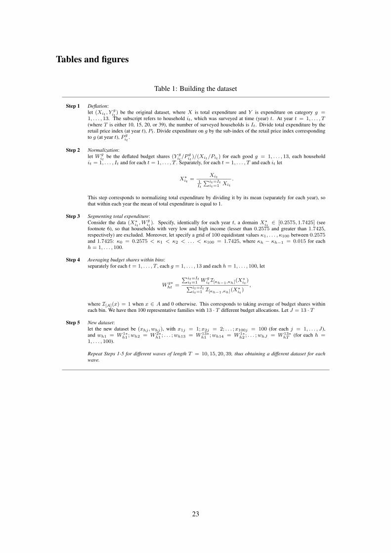
In more detail, our procedure to build the dataset is similar to the one adopted by Kneip (1994)

and consists of five steps, as described in table 1. In the first step, we deflate expenditures using

the retail price indices, so that all the expenditures are converted in real values with 2005 as

base year. In the second step, we take budget shares and normalize total expenditure so that the

value 1 for total expenditure at time t corresponds to mean total expenditure in the year t. In the

third step, we discard data for very rich and very poor household, since they are sparse and not

very reliable: we only keep households whose (normalized) total expenditure ranges within the

interval [0.2575, 1.7425].6 Moreover, we define 100 equidistant bins of width 0.015 within that

interval. In the fourth step, we take, separately for each year and for each expenditure category,

the average budget share within each bin. Finally, in the fifth step, we can build the dataset for

the 100 artificial households, each of them representative of a bin. Since the mean values of

total expenditures within each bin form a set of equidistant and normalized (scale free) numbers,

we simply take the numbers 1, . . . , 100 as their respective values for total expenditures. Each

representative household allocates, for a specific category of expenditure g at year t, a budget

share which is the average of the budget shares allocated by all the households belonging to the

represented bin. For g = 1, . . . , 13 and t = 1, . . . , T we have J = 13 ·T different allocations. We

repeat this procedure for different time windows of length T = 10, 15, 20, 39.

In table 2, we report the average (across households) budget shares for all 13 considered ex-

penditure categories for six different waves. The majority of the budget (about 20%) is spent for

food and housing followed by motoring and leisure services (about 10%). A smaller fraction of

FES contains macro-codes only for the first 6 categories (from housing to clothing and footwear), plus other macro-

categories which are not consistent with the other 7 categories listed above (household goods, household services,

personal goods and services, motoring, fares and other travel, leisure goods, and leisure services). We thus constructed,

for the years 1968-1986, these 7 macro-categories aggregating micro-categories (disaggregate expenditures) in such a

way that they resulted consistent with the way they are formed in the years 1987-2006.5We check also the case of two, three, and four family members and results are similar and available upon request.6The rationale behind these numbers is that, similarly to Kneip (1994), we specify a grid of total expenditure values

0.25 =: X0 < X1 < X2 . . . < Xn < 1.75 =: Xn+1 and we take n = 100 bins of length 0.015 such that each of the

values X1, . . . , Xn lies exactly in the middle.

8

budget is allocated to all other goods and remained constant in time at values less than 10%. When

looking at the three waves of 10 years (columns 2 to 4 in table 2), we notice that while the share

of budget allocated to food has remained constant over time at about 18%, the share allocated to

housing has decreased from 30% to 18%. An increase in the expenditure for motoring from 8% to

13% and leisure services from 5% to 12% is also noticed, a sign of an increased level of welfare

in English population. Finally we notice a decrease in tobacco budget shares from 7% to 2%.

In table 3, we consider the same averages but for more homogeneous classes of normalized

total expenditure xh (as a proxy for income): poor (xh ≤ 30), medium (30 < xh ≤ 70), and rich

(xh > 70) households. While the same time patterns highlighted above remain true for all income

classes, we find differences among households with different income level. Consistently with

Engel’s law in each of the windows considered poor households allocate more budget than rich

to necessities. For example in the time span from 1997 to 2006 poor household allocate to food

24% of their budget against 13% allocated by rich ones, and spend for fuel, light, and power 7%

against just 3% spent by rich families. In the same period poor households allocated less budget

than rich ones to luxuries as motoring (9% against 16%) and leisure services (9% against 15%).

Finally, irrespectively of their income households allocate between 19% and 17% of their budget

to housing and 4% to alcoholic drinks. These across–income differences is what we want to model

and estimate in this paper by means of latent Engel curves. Indeed, already from this descriptive

analysis we can tentatively classify goods according to their budget shares into three broad classes:

necessities (budget shares decreasing with total expenditure), luxuries (budget shares increasing

with total expenditure), and goods for which the budget share is constant with respect to total

expenditure.

4 An approximate factor model for budget shares

As suggested by Bai and Ng (2002), we can consider equation (2) as a factor model withR factors

common to the J budget shares, withR < J . Thus, for every household h we can write the budget

share for expenditure category j as:7

wjh = a′jfh + ejh, j = 1, . . . , J ; h = 1, . . . , H, (3)

7Notice that, given the way our dataset is built (see section 3 for details), the time dimension does not play any role

in this context. Moreover, for simplicity each budget share is rescaled to have zero mean.

9

where aj and fh are R–dimensional vectors of loadings and latent factors respectively. In matrix

notation

w = Af + e, (4)

where w and e are J×H , A is J×R, and f isR×H . We call the term Af the common component

and the term e the idiosyncratic component orthogonal to the factors. While an exact factor model

would require that idiosyncratic components are uncorrelated across expenditure categories, this

is here an unreasonable restriction. Indeed, the adding–up condition of budget shares implies

non-zero cross–correlation both in the common and in the idiosyncratic component. On the other

hand, in approximate factor models a large J allows for mildly correlated idiosyncratic terms. In

fact, a large cross–section of budget shares is what allows us to choose a different modelling and

estimation strategy with respect to Lewbel (1991). Namely, we can apply the theory by Bai and

Ng (2002) in this paper. The necessity of having a large number of items is the practical reason for

pooling expenditures of different years together when building the dataset as described in section

3.

The complete details and assumptions for the approximate factor model are in Bai and Ng

(2002) and we recall here just the three main assumptions:

1. factors: limH→∞1H

∑Hh=1 fhf

′h = Σf , for some positive definite and diagonalR×Rmatrix

Σf ;

2. loadings: limJ→∞ ||A′A/J −D|| = 0, for some positive definite R×R matrix D8;

3. idiosyncratic components: define Σe = E[ehe′h] then there existsM > 0 s.t.

∑Jk=1 |(Σe)jk| ≤

M for any j = 1, . . . , J .

Assumption 1 implies the existence of the covariance matrix of the factors which being diagonal

implies that the factors are orthogonal. Assumption 2 is necessary for identification of the loadings

and implies that, when J goes to infinity, A′A is O(J). Assumption 3 defines an approximate

factor model by allowing for some correlation across goods in the idiosyncratic components, this

is equivalent to require the largest eigenvalue of Σe to be bounded as J goes to infinity (see also

Chamberlain and Rothschild, 1983).

The rank of the considered system of budget shares, is therefore the smallest integer R such

that equation (3) holds. While Lewbel (1991) proposes a test based on LDU decomposition to

8We use the Froboenius norm for a matrix, i.e. ||B|| =√

tr(BB′).

10

determine R, both Kneip (1994) and Donald (1997) propose nonparametric estimation methods.

We instead adopt here the estimation method proposed by Bai and Ng (2002), based on approx-

imate principal component analysis. This approach provides a consistent estimate of R and the

space spanned by the factors when both H and J go to infinity. In the rest of this section we first

briefly review how to estimate factors via principal components and how to determine R. We then

provide an identification strategy based on statistical independence. Finally, by comparing (2) and

(3), we see that the elements of the R-dimensional vector of basic Engel curves g(xh) may be

recovered by regressing each identified factors on total expenditure.

Estimation. First let us assume that R is known, then the estimated factors and loadings are

obtained by solving

(f , A) = arg min(f ,A)

V (R,A, f) = arg min(f ,A)

1

JH

J∑

j=1

H∑

h=1

(wjh − a′jfh)2, (5)

subject to an additional identification condition which consistently with assumption 2, we require

to be A′A/J = IR, where IR is the R-dimensional identity matrix. With this choice, the columns

of A are given by√J-times the eigenvectors corresponding to the R largest eigenvalues of the

sample covariance matrix of the observed budget shares 1H

∑Hh=1whw

′h, where wh is the J-

dimensional vector of budget shares of household h. In the limit J,H → ∞ the estimated loadings

A are a consistent estimate of A and the factors can be consistently estimated as the R largest

principal components: F = A′w/J (see Theorem 1 in Bai and Ng, 2002, for a proof).

Following Bai and Ng (2002), we can use the above estimation method to estimate the number

of factorsR. This can be done by estimating the factors and their loadings for different values k of

the number of factors and by solving each time (5). Define Ak and fk as the approximate principal

components estimates of loadings and factors when assuming the existence of k common factors.

The estimated number of factors is the value of k that minimizes this function, conveniently pe-

nalized with a penalty function p(k, J,H) that depends both on J and on H . We thus look for

minima of the ICs criteria proposed by Bai and Ng (2002), i.e.

R = arg min1≤k≤kmax

log V (k, Ak, fk) + p(k, J,H) (6)

11

where

p(k, J,H) = k

(J +H

JH

)log

(JH

J +H

)

or (7)

p(k, J,H) = k

(J +H

JH

)log(min

(√J,

√H))2

.

Provided that we have a consistent estimate of the factors and their loadings, Bai and Ng (2002)

prove consistency of R as J,H → ∞. In the following sections we also apply two other methods.

A refinement of the above information criteria proposed by Alessi et al. (2010) where a fine–tuning

parameter in the penalty function is introduced. A test by Onatski (2010) which is instead based

on the asymptotic distribution of the eigenvalues of the sample covariance matrix.

Identification. Factor models have an indeterminacy which they cannot solve: both the estimated

loading matrix A and factors f are asymptotically consistent estimates of the true ones only up

to an orthogonal transformation. We have, therefore, an identification problem which makes dif-

ficult the economic interpretation of the estimated factors. In order to identify the model, we use

independent component analysis (ICA) which requires two further assumptions on the R latent

factors:

4. the components of the factor vector fh are mutually independent, i.e. the joint probability

density of the factors is given by

D(fh) =R∏

r=1

dr(frh), h = 1 . . . , H,

where dr is the marginal probability density of the r-th factor;

5. the marginal densities dr are non–Gaussian, for all i = 1, . . . , R, with the exception of at

most one.

Assumption 4 is justified on the basis of the fact that the latent factors represent the basic latent

Engel curves generating the observed system of Engel curves. These basic functions, in turn, have

characteristics which reflect fundamental aspects of human behaviours driving consumption deci-

sions. As argued by Witt (2001), consumption decisions are ultimately driven by basic needs and

acquired wants. Therefore, assuming that latent factors are independent amounts to claim that the

set of needs and wants associated with each factor is of fundamental different nature, i.e. generates

an independent pattern, from the set of needs and wants associated with the other factors. For ex-

ample, if a factor reflects a pattern associated with necessities and another factor reflects a pattern

12

associated with luxuries, these two factors can be seen as statistical independent, because neces-

sities mainly reflect physiological needs, while luxuries reflect culturally acquired wants such as

social recognition and status. The drivers underlying consumption decisions about necessities and

luxuries react in an independent way to changes in income: for example, physiological needs tend

rapidly to satiate, as income gives the possibility to satisfy these needs, whereas acquired wants

such as social recognition and status may be even increasingly reinforced, as income increases.

Nevertheless, it has to be stressed that while basic Engel curves reflect independent motives for

consumption, the observed Engel curves can be seen as a mixture of these needs and thus their

joint distribution may have a non–trivial dependence structure.

Assumption 5 is justified by testing for normality in the data and also by noticing that often data

on consumption expenditures are non-Gaussian (see e.g. Fagiolo et al., 2010) and, moreover, being

budget shares defined on the unit interval, they must have a distribution with bounded support (e.g.

a beta distribution) hence not a Gaussian distribution. As a consequence also the joint distribution

of the factors is non–Gaussian.

ICA can been seen as an extension or a strengthening of principal component analysis (PCA)

(see Comon, 1994; Hyvarinen et al., 2001; Bonhomme and Robin, 2009). Indeed, while PCA

gives a transformation of the original space such that the computed latent factors are linearly un-

correlated, ICA goes further by attempting to minimize all statistical dependencies between the

resulting components. One can show that if there exists a representation with non-Gaussian, statis-

tically independent components, then the representation is essentially unique (up to a permutation,

a sign, and a scaling factor) (Comon, 1994). There exist a number of computationally efficient

algorithms for consistent estimation (Hyvarinen et al., 2001). This identification method is partic-

ularly appealing since it is purely data–driven and not based on economic assumptions which in

turn would require micro–funded models of consumption behavior.

The most popular ICA algorithms are: Joint Approximate Diagonalization of Eigen-matrices

(JADE by Cardoso and Souloumiac, 1993), Fast Fixed-Point Algorithm (FastICA by Hyvarinen

and Oja, 2000). Both methods are based on two steps: i) a whitening step achieved by PCA, in

which the data are transformed so that the covariance matrix is diagonal and has reduced rank,

i.e. we get rid of the idiosyncratic component; ii) a source separation step in which the orthogonal

transformation necessary for achieving identification is determined.

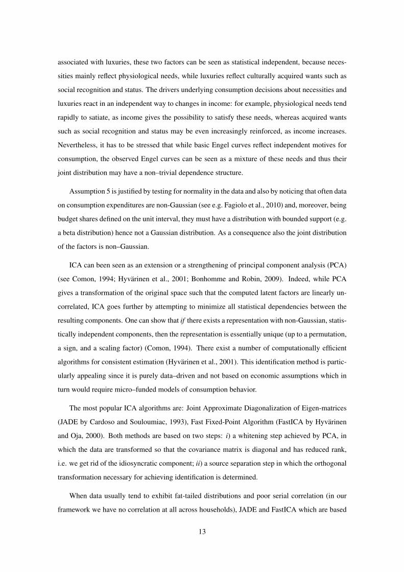
When data usually tend to exhibit fat-tailed distributions and poor serial correlation (in our

framework we have no correlation at all across households), JADE and FastICA which are based

13

on non-Gaussianity of the data, hence on higher order moments, are the most used algorithms.9

We present here results obtained with JADE, the results obtained with FastICA being similar.

Once estimation of the common component is accomplished via approximate PCA, we are left

with a first estimate of the factors fh for any household h. JADE looks for an orthogonal J × R

matrix U such that the identified factors fh = U′fh are maximally non-Gaussian distributed. A

set of random vectors is mutually independent if all the cross-cumulants (i.e. the coefficients of

the Taylor series expansion of the log of the moment generating function) of order higher than

two are equal to zero. In particular, Cardoso and Souloumiac (1993) prove that the factors fh are

maximally independent if their associated fourth-order cumulant tensor which is a R × R matrix

is maximally diagonal.10 JADE is a very efficient algorithm in low dimensional problems as the

one treated here (we have few factors), while a higher computational cost is required when the

dimension increases.

Once we apply JADE the estimated and identified factors, fh, are identified up to a permutation,

a sign, and a scaling factor. The order of the factor is irrelevant for our purposes. Moreover, given

that independent components are nothing else but weighted averages of the data, the sign is chosen

to be consistent with the average of budget shares across goods. Finally, the scale is determined in

such a way that the identified loadings A satisfy A′A/J = IR.

5 Estimation of the basic Engel curves

By combining (3) and (2) we can think of the following system of equations

wjh =

R∑

r=1

ajrfrh + ejh, j = 1, . . . , J ; h = 1, . . . , H,

frh = gr(xh) + zrh, r = 1, . . . , R, (8)

where we introduced an error term in the specification of the latent factors such that zrh ∼

i.i.d.(0, 1). The aim of this section is to provide consistent estimators of the basic Engel curves

gr(xh). In what follows we propose a non–parametric and a parametric estimator of these curves.

While the former is appealing since it is purely data driven, the latter allows us to relate our results

9Another algorithm is Second-Order Blind Identification (SOBI Belouchrani et al., 1997), which, although usu-

ally applied in time-series analysis, could be extended to cross-sectional data with correlations among observations.

However, this is not the case for us, as we assume no correlations across households.10While the cumulant depends on four indexes the cumulant tensor depends on two indexes, the other two being

canceled by means of an additional arbitrary matrix. We thus have to consider several cumulant matrices which have to

be jointly diagonalized. See the appendix for a short description of the JADE algorithm.

14

with the existing literature on functional forms of Engel curves (see e.g. Lewbel, 1991; Banks

et al., 1997).

Proposition 1. The non–parametric estimator for the basic Engel curve gr(xh) is defined as

γ∗r (xh), such that

γ∗r (xh) = argmaxγr

H∑

k=1

[frk − γr − δr(xk − xh)

]2KbH (xk − xh) , r = 1, . . . , R, (9)

where KbH (·) is a suitable kernel function depending on a bandwidth bH (see assumption K in the

appendix). Then,

p- limJ,H→∞

|γ∗r (xh)− gr(xh)|2 = 0,

with a rate of convergence given by min(J−1, H−1b−1

H , bHH−1).

Proof: see the appendix.

Few remarks are necessary. The proposed estimator is a local linear estimator as defined for

example in Fan and Gijbels (1992) and Fan (1993). An alternative estimator is represented by the

local constant fit defined as,

γ∗r (xh) = argmaxγr

H∑

k=1

[frk − γr

]2wk(bH), r = 1, . . . , R. (10)

From (10), we can have either the Nadaraya–Watson estimator (see e.g. Watson, 1964) when

wk(bH) = KbH (xk−xh) or the Gasser–Muller estimator (see e.g. Gasser and Muller, 1984) when

wk(bH) =∫KbH (u − xh)du. Both (9) and (10) would satisfy Proposition 1. However, it can

be proved that the local linear estimator (9) has a smaller finite sample bias, is asymptotically

efficient, and has a better behavior at the extremes of the sample (see e.g. Fan and Gijbels, 2003,

for a comparison). Moroever, by solving the maximization in (9), we obtain also a local estimate of

the slope δ∗r (xh) which is an estimate of the first derivative of the basic Engle curves. Consistency

of the latter in our framework is proved exactly in the same way as in Proposition 1.

The choice of the bandwidth can be based on different methods. In our estimations below

(see next section) we choose the bandwidth on the basis of the minimization of a polynomial

approximation of the mean integrated square error (of γ∗r (xh)), following the approach proposed

by Fan and Gijbels (2003, Section 4.2).

In order to compare our results with the literature (Lewbel, 1991; Banks et al., 1997), we

also investigate which functional form of total expenditure better fits each identified factor. Thus

15

instead of (9) we can think of a parametric model for the basic Engel curves:

gr(xh) = αr + βrm(xh), r = 1, . . . , R; h = 1, . . . , H. (11)

We estimate the following functions m(xh) of total expenditure: xh, x2h, x−1h , x−2

h , log xh,

(log xh)2, xh log xh. These are are the functional forms also considered by Lewbel (1991) and

Donald (1997). By substituting (11) into (8) we have

frh = αr + βrm(xh) + zrh, r = 1, . . . , R; h = 1, . . . , H. (12)

The unknown parameters can be estimated by ordinary least squares with the caveat that, since

zrh are non-Gaussian by assumption 5, robust standard errors must be computed. If the factors

frh were observed, consistency of the estimated parameters would follow from Quasi Maximum

Likelihood theory. However, since frh are unobserved and must be replaced by their estimates

frh, we have to use lemma 1 in appendix and consistency is achieved provided that both H and J

tend to infinity. We have the following result.

Proposition 2. Define the matrix of explanatory variables and the vector of unknown parameters

X = (1H ,m(x)), θr =

(αr

βr

), r = 1, . . . , R,

where 1H is an H-dimensional column vector of ones and x = (x1 . . . xH)′. The estimated vector

parameters for the r-th basic Engel curve is given by

θ∗r = (X ′X )−1X ′fr,

such that

p- limJ,H→∞

|θ∗r − θr| = 0, r = 1, . . . , R,

with a rate of convergence given by min(J−1, H−1

).

Proof: see the appendix.

6 Results

Number of factors. Table 4 displays the estimates of the number of factors for time windows

of 10, 15, and 20 years length plus the whole sample length of 39 years. We find between 2

and 4 common factors, the average of the criteria being always between 2 and 3. In the following

analysis the main role is played by the first two largest factors, while a third plays a minor although

theoretical important role. Adding more factors does not change the interpretation and therefore

we present results for R = 3.

16

In the last 3 columns of table 4 we show the proportion of variance explained by each factor.

The first factor explains, for all the time windows considered, always between 50% and 60% of

total variance, being clearly the most important. Its contribution to the total variance of budget

shares, however, decreased with time. This is probably due to the fact that in the last thirty or forty

years families of the same income class have increasingly differentiated their consumption habits,

so that idiosyncratic components have played a relatively bigger role. This may in turn be due to

a wider range of products available joint with an increase in families’ total resources. Moreover,

as the first factor will be interpreted as related to necessities (see section 4), a decrease in the

explained variance of the first factor can also be seen as a sign of an increased level of welfare, as

mentioned above.

Factor models are identified under a specific condition on diverging eigenvalues of the covari-

ance matrix of the data (see assumption 3). This is precisely the assumption tested by the Bai and

Ng (2002) criterion which shows evidence of an additional one or even two less important, but

still common, factors explaining a much lower proportion of variance, in fact lower than 10%. We

must stress the fact that not recognizing the existence of such factors would imply the existence

of common features in the idiosyncratic components. Indeed, in order to be truly common the

factors do not have to be necessarily large (a relative concept) in terms of explained variance, but

they have to be pervasive, a well defined feature that can be measured by studying the asymptotic

behaviour of eigenvalues. This is exactly what the employed criteria do.

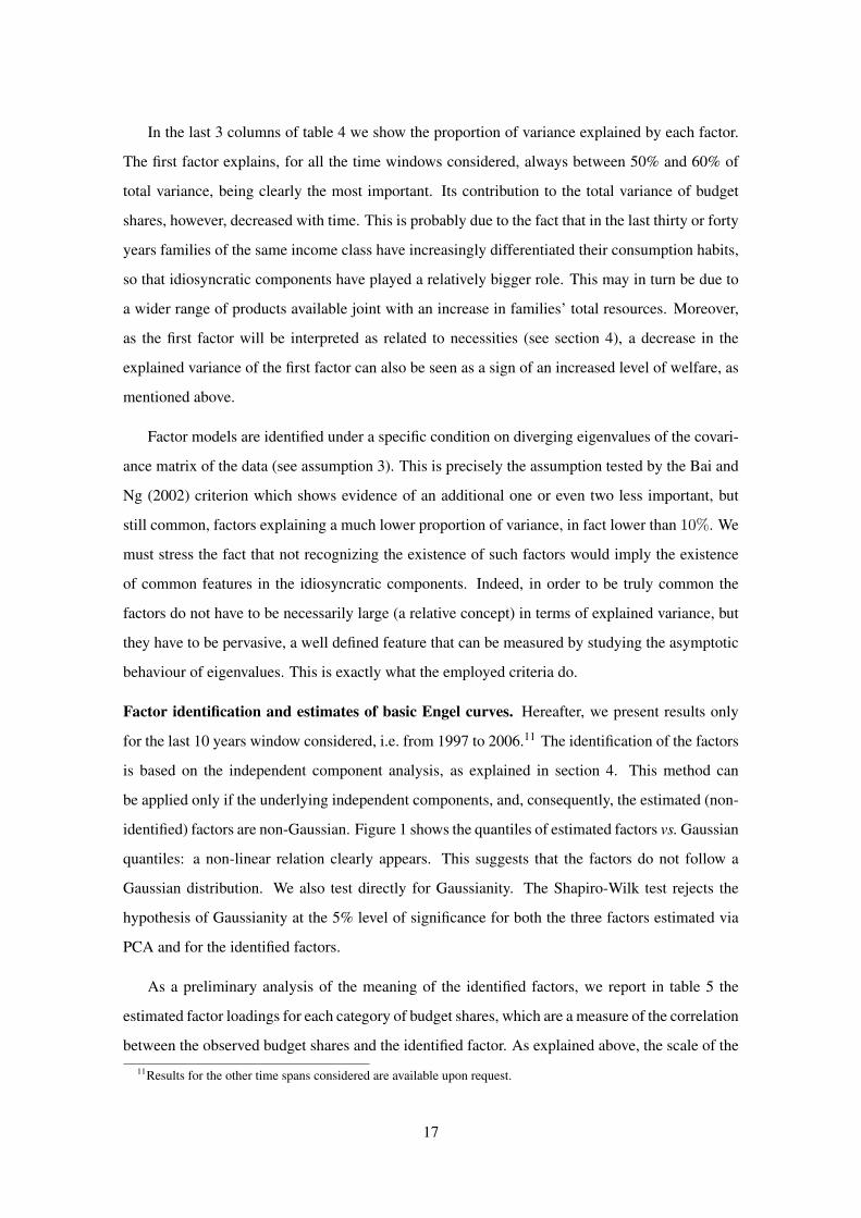
Factor identification and estimates of basic Engel curves. Hereafter, we present results only

for the last 10 years window considered, i.e. from 1997 to 2006.11 The identification of the factors

is based on the independent component analysis, as explained in section 4. This method can

be applied only if the underlying independent components, and, consequently, the estimated (non-

identified) factors are non-Gaussian. Figure 1 shows the quantiles of estimated factors vs. Gaussian

quantiles: a non-linear relation clearly appears. This suggests that the factors do not follow a

Gaussian distribution. We also test directly for Gaussianity. The Shapiro-Wilk test rejects the

hypothesis of Gaussianity at the 5% level of significance for both the three factors estimated via

PCA and for the identified factors.

As a preliminary analysis of the meaning of the identified factors, we report in table 5 the

estimated factor loadings for each category of budget shares, which are a measure of the correlation

between the observed budget shares and the identified factor. As explained above, the scale of the

11Results for the other time spans considered are available upon request.

17

loadings vector is fixed according to the normalization A′A/J = IR. We find that the first

factor is highly correlated with food and fuel, light and power budget shares. This again suggests

that the first factor captures consumption patterns typically associated with the Engel’s law: as

total expenditure rises, budget shares decrease, the downward trend being more dramatic for the

lowest levels of income. On the other hand the second factor is mostly correlated with luxuries

as motoring and leisure services, while the third displays the highest correlation with food and

housing expenditures.

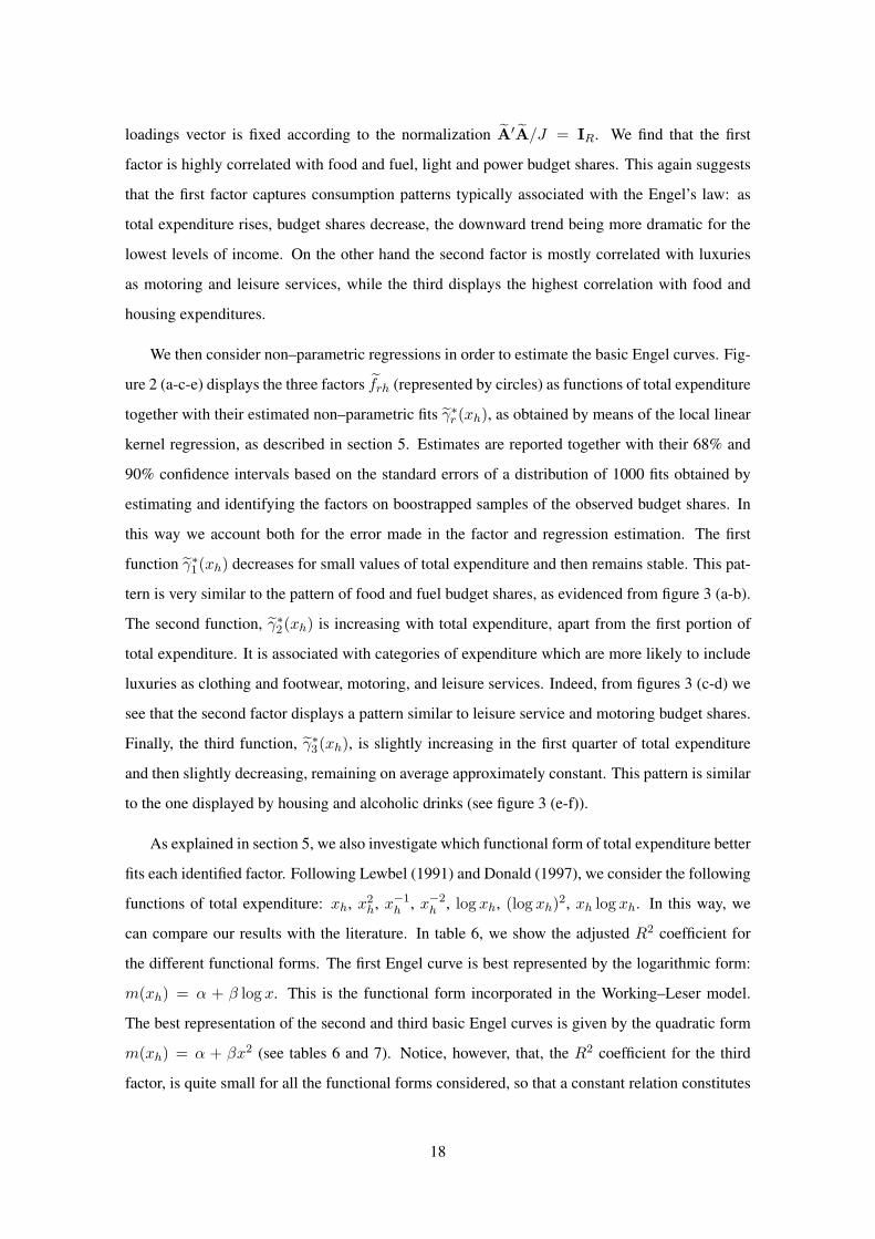
We then consider non–parametric regressions in order to estimate the basic Engel curves. Fig-

ure 2 (a-c-e) displays the three factors frh (represented by circles) as functions of total expenditure

together with their estimated non–parametric fits γ∗r (xh), as obtained by means of the local linear

kernel regression, as described in section 5. Estimates are reported together with their 68% and

90% confidence intervals based on the standard errors of a distribution of 1000 fits obtained by

estimating and identifying the factors on boostrapped samples of the observed budget shares. In

this way we account both for the error made in the factor and regression estimation. The first

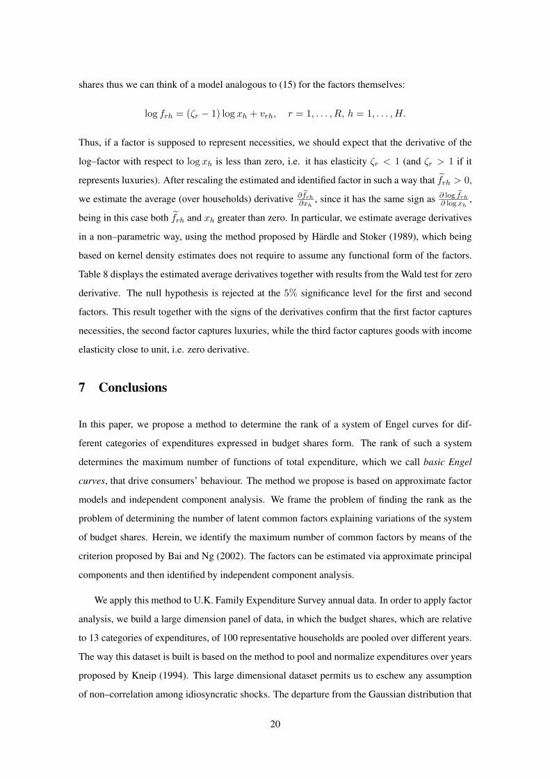
function γ∗1(xh) decreases for small values of total expenditure and then remains stable. This pat-

tern is very similar to the pattern of food and fuel budget shares, as evidenced from figure 3 (a-b).

The second function, γ∗2(xh) is increasing with total expenditure, apart from the first portion of

total expenditure. It is associated with categories of expenditure which are more likely to include

luxuries as clothing and footwear, motoring, and leisure services. Indeed, from figures 3 (c-d) we

see that the second factor displays a pattern similar to leisure service and motoring budget shares.

Finally, the third function, γ∗3(xh), is slightly increasing in the first quarter of total expenditure

and then slightly decreasing, remaining on average approximately constant. This pattern is similar

to the one displayed by housing and alcoholic drinks (see figure 3 (e-f)).

As explained in section 5, we also investigate which functional form of total expenditure better

fits each identified factor. Following Lewbel (1991) and Donald (1997), we consider the following

functions of total expenditure: xh, x2h, x−1h , x−2

h , log xh, (log xh)2, xh log xh. In this way, we

can compare our results with the literature. In table 6, we show the adjusted R2 coefficient for

the different functional forms. The first Engel curve is best represented by the logarithmic form:

m(xh) = α + β log x. This is the functional form incorporated in the Working–Leser model.

The best representation of the second and third basic Engel curves is given by the quadratic form

m(xh) = α + βx2 (see tables 6 and 7). Notice, however, that, the R2 coefficient for the third

factor, is quite small for all the functional forms considered, so that a constant relation constitutes

18

also a good approximation. This is also confirmed from the analysis of the estimated coefficients

in table 7. Moreover, we notice that the first factor is the most important when considering only

poor households, while the second prevails when considering households with medium levels of

income. For the richest households considered no fit is significant and this is due to the high

dispersion of budget shares at the right extreme of the income distribution.

Summing up, the parametric specification of the system of basic Engel curves which is most

consistent with our findings is:

wjh = c1j + c2j log xh + c3jx2h + ejh, j = 1, . . . , J, h = 1, . . . , H, (13)

where crj in our framework are combinations of the loadings ajr and the coefficients αr and βr

for r = 1, 2, 3. The functional form (13) is consistent with the one proposed by Lewbel (1997):

wjh = c1j + c2j log xh + c3jψ(xh) + ejh, j = 1, . . . , J, h = 1, . . . , H, (14)

where ψ is some non-linear function of total expenditure. Banks et al. (1997), using 1980-1982

U.K. FES data, found that Engel curves have indeed the form of equation (14), with ψ(xh) =

(log xh)2. In this latter respect, our results slightly differ from previous findings, since our last

term is quadratic in xh and not in log xh.

Derivatives of basic Engel curves. A final way to interpret the factors is based on the estimation

of the derivatives of the basic Engel curves. Indeed, the sign of these functions is strictly connected

to whether a category of expenditure should be classified as luxury or necessity. In figure 2 (b-

d-f) we show the derivatives of the basic Engel curves δ∗r (xh), estimated with a local–linear fit

as explained in Proposition 1 together with 68% and 90% boostrapped confidence intervals. In

agreement with the findings above, the first derivative of the first basic Engel curve is negative

for low and medium income families as predicted from the Engel law for necessary goods. The

derivative of the second Engel curve captures luxuries being positive for medium–high income

households, while the derivative of the third curve it is zero for all households indicating a constant

Engel curve.

Moreover, total expenditure elasticity ǫj of good j has a direct connection with the double log

model, since for any category of expenditure j we can write (see Deaton and Muellbauer, 1980, p.

17):

logwjh = (ǫj − 1) log xh + νjh, j = 1, . . . , J, h = 1, . . . , H, (15)

where νjh is an error term. In our framework, the latent factors are weighted averages of budget

19

shares thus we can think of a model analogous to (15) for the factors themselves:

log frh = (ζr − 1) log xh + vrh, r = 1, . . . , R, h = 1, . . . , H.

Thus, if a factor is supposed to represent necessities, we should expect that the derivative of the

log–factor with respect to log xh is less than zero, i.e. it has elasticity ζr < 1 (and ζr > 1 if it

represents luxuries). After rescaling the estimated and identified factor in such a way that frh > 0,

we estimate the average (over households) derivative ∂frh∂xh

, since it has the same sign as ∂ log frh∂ log xh

,

being in this case both frh and xh greater than zero. In particular, we estimate average derivatives

in a non–parametric way, using the method proposed by Hardle and Stoker (1989), which being

based on kernel density estimates does not require to assume any functional form of the factors.

Table 8 displays the estimated average derivatives together with results from the Wald test for zero

derivative. The null hypothesis is rejected at the 5% significance level for the first and second

factors. This result together with the signs of the derivatives confirm that the first factor captures

necessities, the second factor captures luxuries, while the third factor captures goods with income

elasticity close to unit, i.e. zero derivative.

7 Conclusions

In this paper, we propose a method to determine the rank of a system of Engel curves for dif-

ferent categories of expenditures expressed in budget shares form. The rank of such a system

determines the maximum number of functions of total expenditure, which we call basic Engel

curves, that drive consumers’ behaviour. The method we propose is based on approximate factor

models and independent component analysis. We frame the problem of finding the rank as the

problem of determining the number of latent common factors explaining variations of the system

of budget shares. Herein, we identify the maximum number of common factors by means of the

criterion proposed by Bai and Ng (2002). The factors can be estimated via approximate principal

components and then identified by independent component analysis.

We apply this method to U.K. Family Expenditure Survey annual data. In order to apply factor

analysis, we build a large dimension panel of data, in which the budget shares, which are relative

to 13 categories of expenditures, of 100 representative households are pooled over different years.

The way this dataset is built is based on the method to pool and normalize expenditures over years

proposed by Kneip (1994). This large dimensional dataset permits us to eschew any assumption

of non–correlation among idiosyncratic shocks. The departure from the Gaussian distribution that

20

budget shares display and a hypothesis about the nature of the fundamental drivers of consumption

decisions permit us to apply independent component analysis to achieve identification.

Once the common latent factors are identified, we study their properties by means of local–

linear nonparametric regressions which are consistent estimates of the basic Engel curves. To

compare our results with the existing literature we also estimate parametric models the factors as

non–linear functions of total expenditure. Finally, we estimate the first derivatives of the basic

Engel curves by applying local–linear regressions and the method proposed by Hardle and Stoker

(1989). All results show that the observed system of budget shares is well represented by the sum

of a logarithmic, quadratic, and constant basic Engel curves, in a form which is consistent with the

model suggested by Lewbel (1997). Moreover, the three sources of consumption variation reflect

those consumption behaviours typical of expenditures for necessities, luxuries, and unity elasticity

goods.

References

Alessi, L., M. Barigozzi, and M. Capasso (2010). Improved penalization for determining the number of factors in

approximate static factor models. Statistics and Probability Letters 80.

Aversi, R., G. Dosi, G. Fagiolo, M. Meacci, and C. Olivetti (1999). Demand dynamics with socially evolving prefer-

ences. Industrial and Corporate Change 8, 353–468.

Bai, J. and S. Ng (2002). Determining the number of factors in approximate factor models. Econometrica 70, 191–221.

Banerjee, A. and E. Duflo (2011). Poor economics: a radical rethinking of the way to fight global poverty. Public

Affairs.

Banks, J., R. Blundell, and A. Lewbel (1997). Quadratic Engel curves and consumer demand. Review of Economics

and Statistics 79, 527–539.

Belouchrani, A., K. Abed Meraim, J. Cardoso, and E. Moulines (1997). A blind source separation tecnique based on

second order statistics. IEEE Transactions on Signal Processing 45.

Bonhomme, S. and J. Robin (2009). Consistent noisy independent component analysis. Journal of Econometrics 149,

12–25.

Cardoso, J. and A. Souloumiac (1993). Blind beamforming for non-Gaussian signals. IEE Proceedings part F Radar

and Signal Processing 140, 362–362.

Chai, A. and A. Moneta (2010). Retrospectives engel curves. The Journal of Economic Perspectives 24(1), 225–240.

Chamberlain, G. and M. Rothschild (1983). Arbitrage, factor structure and mean-variance analysis in large asset

markets. Econometrica 51, 1305–1324.

Comon, P. (1994). Independent component analysis, a new concept? Signal processing 36, 287–314.

Deaton, A. and J. Muellbauer (1980). An almost ideal demand system. American Economic Review 70, 312–326.

Donald, S. (1997). Inference concerning the number of factors in a multivariate nonparamentric relationship. Econo-

metrica 65, 103–132.

Doz, C., D. Giannone, and L. Reichlin (2011a). A quasi maximum likelihood approach for large approximate dynamic

factor models. Review of Economics and Statistics. forthcoming.

21

Doz, C., D. Giannone, and L. Reichlin (2011b). A two-step estimator for large approximate dynamic factor models

based on Kalman filtering. Journal of Econometrics. forthcoming.

Engel, E. (1857). Die Productions- und Consumtionsverhaltnisse des Konigreichs Sachsen. Bulletin de lInstitut Inter-

national de la Statistique (9).

Fagiolo, G., L. Alessi, M. Barigozzi, and M. Capasso (2010). On the distributional properties of household consumption

expenditures: The case of Italy. Empirical Economics 38.

Fan, J. (1993). Local linear regression smoothers and their minimax efficiency. Annals of Statistics 21, 196–216.

Fan, J. and I. Gijbels (1992). Variable bandwidth and local linear regression smoothers. Annals of Statistics 20, 2008–

2036.

Fan, J. and I. Gijbels (2003). Local Polynomial Modelling and Its Applications. Chapam & HallCRC.

Foellmi, R. and J. Zweimuller (2008). Structural change, engel’s consumption cycles and kaldor’s facts of economic

growth. Journal of Monetary Economics 55(7), 1317–1328.

Forni, M., M. Hallin, M. Lippi, and L. Reichlin (2000). The generalized dynamic-factor model: Identification and

estimation. Review of Economics and Statistics 82, 540–554.

Gasser, T. and G. Muller, H (1984). Estimating regression functions and their derivatives by the kernel method. Scan-

dinavian Journal of Statistics 11, 171–185.

Gorman, W. M. (1981). Some Engel curves. In A. Deaton (Ed.), Essays in the Theory and Measurements of Consumer

Behaviour in Honor of Sir Richard Stone. Cambridge University Press.

Gourieroux, C., A. Monfort, and A. Trognon (1984). Pseudo maximum likelihood methods: Theory. Economet-

rica 52(3), 681–700.

Hardle, W. and T. Stoker (1989). Investigating smooth multiple regression by the method of average derivatives. Journal

of the American Statistical Association 84, 986–995.

Hyvarinen, A., J. Karhunen, and E. Oja (2001). Independent Component Analysis. Wiley.

Hyvarinen, A. and E. Oja (2000). Independent component analysis: Algorithms and applications. Neural Networks 13,

411–430.

Kneip, A. (1994). Nonparametric estimation of common regressors for similar curve data. The Annals of Statistics 22,

1386–1427.

Lewbel, A. (1991). The rank of demand systems: Theory and nonparametric estimation. Econometrica 59, 711–730.

Lewbel, A. (1997). Consumer demand systems and household equivalence scales. Handbook of Applied Econometrics:

Microeconomics 2, 167–201.

Onatski, A. (2010). Determining the number of factors form empirical distribution of eigenvalues. Review of Economics

and Statistics. forthcoming.

Pasinetti, L. (1981). Structural change and economic growth: a theoretical essay on the dynamics of the wealth of

nations. Cambridge University Press.

Stock, J. and M. Watson (1989). New indexes of coincident and leading economic indicators. NBER macroeconomics

annual, 351–394.

Watson, G. S. (1964). Smooth regression analysis. Sankhya 26, 359–372.

Witt, U. (1999). Bioeconomics as economics from a darwinian perspective. Journal of Bioeconomics 1(1), 19–34.

Witt, U. (2001). Learning to consume–A theory of wants and the growth of demand. Journal of Evolutionary Eco-

nomics 11, 23–36.

22

Tables and figures

Table 1: Building the dataset

Step 1 Deflation:

let (Xit , Ygit) be the original dataset, where X is total expenditure and Y is expenditure on category g =

1, . . . , 13. The subscript refers to household it, which was surveyed at time (year) t. At year t = 1, . . . , T(where T is either 10, 15, 20, or 39), the number of surveyed households is It. Divide total expenditure by the

retail price index (at year t), Pt. Divide expenditure on g by the sub-index of the retail price index corresponding

to g (at year t), P git

.

Step 2 Normalization:

let W git

be the deflated budget shares (Y git/P g

it)/(Xit/Pit ) for each good g = 1, . . . , 13, each household

it = 1, . . . , It and for each t = 1, . . . , T . Separately, for each t = 1, . . . , T and each it let

X∗

it=

Xit

1It

∑it=Itit=1 Xit

.

This step corresponds to normalizing total expenditure by dividing it by its mean (separately for each year), so

that within each year the mean of total expenditure is equal to 1.

Step 3 Segmenting total expenditure:

Consider the data (X∗

it,W g

it). Specify, identically for each year t, a domain X∗

it∈ [0.2575, 1.7425] (see

footnote 6), so that households with very low and high income (lesser than 0.2575 and greater than 1.7425,

respectively) are excluded. Moreover, let specify a grid of 100 equidistant values κ1, . . . , κ100 between 0.2575and 1.7425: κ0 = 0.2575 < κ1 < κ2 < . . . < κ100 = 1.7425, where κh − κh−1 = 0.015 for each

h = 1, . . . , 100.

Step 4 Averaging budget shares within bins:

separately for each t = 1, . . . , T , each g = 1, . . . , 13 and each h = 1, . . . , 100, let

W g∗ht

=

∑it=Itit=1 W g

itI[κh−1,κh](X

∗

it)

∑it=Itit=1 I[κh−1,κh](X

∗

it)

,

where I[A](x) = 1 when x ∈ A and 0 otherwise. This corresponds to taking average of budget shares within

each bin. We have then 100 representative families with 13 · T different budget allocations. Let J = 13 · T

Step 5 New dataset:

let the new dataset be (xhj , whj), with x1j = 1;x2j = 2; . . . ;x100j = 100 (for each j = 1, . . . , J),

and wh1 = W 1∗h1 ;wh2 = W 2∗

h1 ; . . . ;wh13 = W 13∗h1 ;wh14 = W 1∗

h2 ; . . . ;whJ = W 13∗hT

(for each h =1, . . . , 100).

Repeat Steps 1-5 for different waves of length T = 10, 15, 20, 39, thus obtaining a different dataset for each

wave.

23

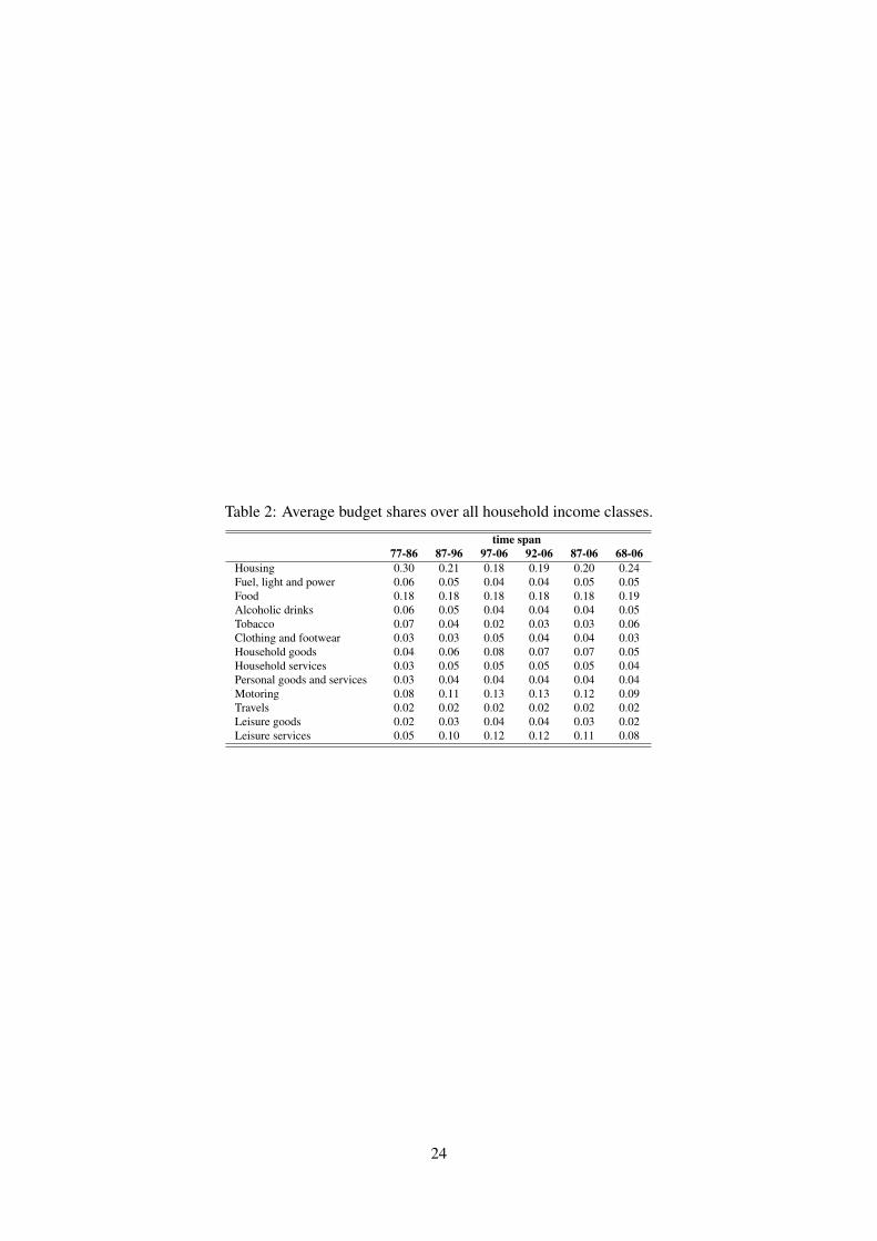
Table 2: Average budget shares over all household income classes.

time span

77-86 87-96 97-06 92-06 87-06 68-06

Housing 0.30 0.21 0.18 0.19 0.20 0.24

Fuel, light and power 0.06 0.05 0.04 0.04 0.05 0.05

Food 0.18 0.18 0.18 0.18 0.18 0.19

Alcoholic drinks 0.06 0.05 0.04 0.04 0.04 0.05

Tobacco 0.07 0.04 0.02 0.03 0.03 0.06

Clothing and footwear 0.03 0.03 0.05 0.04 0.04 0.03

Household goods 0.04 0.06 0.08 0.07 0.07 0.05

Household services 0.03 0.05 0.05 0.05 0.05 0.04

Personal goods and services 0.03 0.04 0.04 0.04 0.04 0.04

Motoring 0.08 0.11 0.13 0.13 0.12 0.09

Travels 0.02 0.02 0.02 0.02 0.02 0.02

Leisure goods 0.02 0.03 0.04 0.04 0.03 0.02

Leisure services 0.05 0.10 0.12 0.12 0.11 0.08

24

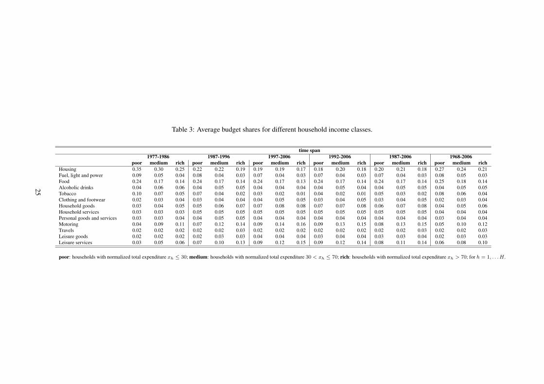
Table 3: Average budget shares for different household income classes.

time span

1977-1986 1987-1996 1997-2006 1992-2006 1987-2006 1968-2006

poor medium rich poor medium rich poor medium rich poor medium rich poor medium rich poor medium rich

Housing 0.35 0.30 0.25 0.22 0.22 0.19 0.19 0.19 0.17 0.18 0.20 0.18 0.20 0.21 0.18 0.27 0.24 0.21

Fuel, light and power 0.09 0.05 0.04 0.08 0.04 0.03 0.07 0.04 0.03 0.07 0.04 0.03 0.07 0.04 0.03 0.08 0.05 0.03

Food 0.24 0.17 0.14 0.24 0.17 0.14 0.24 0.17 0.13 0.24 0.17 0.14 0.24 0.17 0.14 0.25 0.18 0.14

Alcoholic drinks 0.04 0.06 0.06 0.04 0.05 0.05 0.04 0.04 0.04 0.04 0.05 0.04 0.04 0.05 0.05 0.04 0.05 0.05

Tobacco 0.10 0.07 0.05 0.07 0.04 0.02 0.03 0.02 0.01 0.04 0.02 0.01 0.05 0.03 0.02 0.08 0.06 0.04

Clothing and footwear 0.02 0.03 0.04 0.03 0.04 0.04 0.04 0.05 0.05 0.03 0.04 0.05 0.03 0.04 0.05 0.02 0.03 0.04

Household goods 0.03 0.04 0.05 0.05 0.06 0.07 0.07 0.08 0.08 0.07 0.07 0.08 0.06 0.07 0.08 0.04 0.05 0.06

Household services 0.03 0.03 0.03 0.05 0.05 0.05 0.05 0.05 0.05 0.05 0.05 0.05 0.05 0.05 0.05 0.04 0.04 0.04

Personal goods and services 0.03 0.03 0.04 0.04 0.05 0.05 0.04 0.04 0.04 0.04 0.04 0.04 0.04 0.04 0.04 0.03 0.04 0.04

Motoring 0.04 0.09 0.11 0.07 0.12 0.14 0.09 0.14 0.16 0.09 0.13 0.15 0.08 0.13 0.15 0.05 0.10 0.12

Travels 0.02 0.02 0.02 0.02 0.02 0.03 0.02 0.02 0.02 0.02 0.02 0.02 0.02 0.02 0.03 0.02 0.02 0.03

Leisure goods 0.02 0.02 0.02 0.02 0.03 0.03 0.04 0.04 0.04 0.03 0.04 0.04 0.03 0.03 0.04 0.02 0.03 0.03

Leisure services 0.03 0.05 0.06 0.07 0.10 0.13 0.09 0.12 0.15 0.09 0.12 0.14 0.08 0.11 0.14 0.06 0.08 0.10

poor: households with normalized total expenditure xh ≤ 30; medium: households with normalized total expenditure 30 < xh ≤ 70; rich: households with normalized total expenditure xh > 70; for h = 1, . . . H .

25

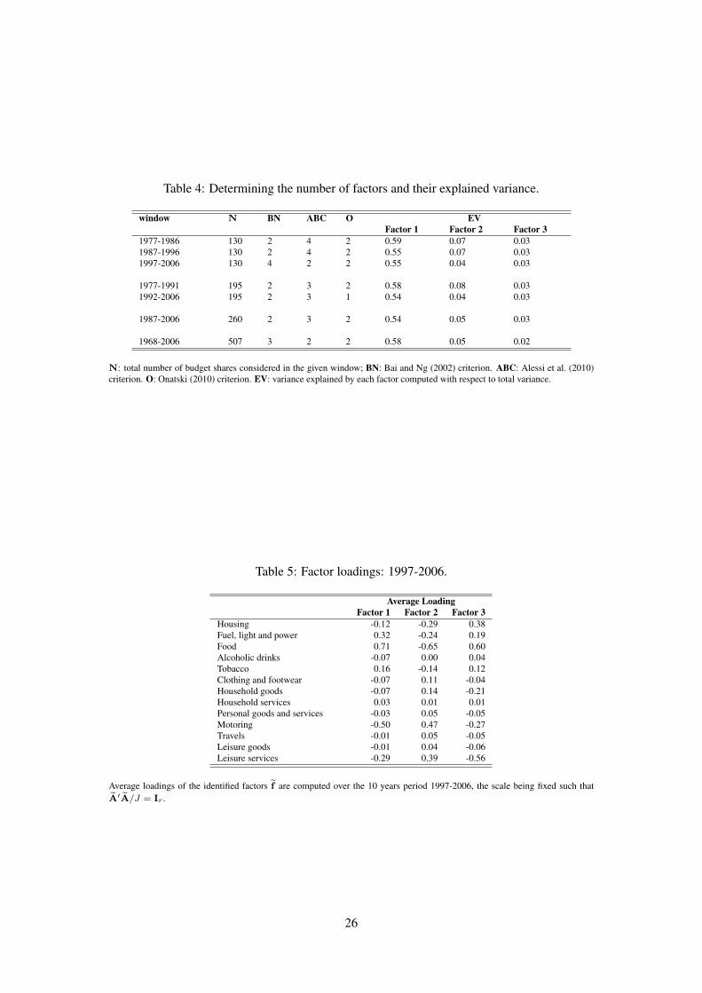
Table 4: Determining the number of factors and their explained variance.

window N BN ABC O EV

Factor 1 Factor 2 Factor 3

1977-1986 130 2 4 2 0.59 0.07 0.03

1987-1996 130 2 4 2 0.55 0.07 0.03

1997-2006 130 4 2 2 0.55 0.04 0.03

1977-1991 195 2 3 2 0.58 0.08 0.03

1992-2006 195 2 3 1 0.54 0.04 0.03

1987-2006 260 2 3 2 0.54 0.05 0.03

1968-2006 507 3 2 2 0.58 0.05 0.02

N: total number of budget shares considered in the given window; BN: Bai and Ng (2002) criterion. ABC: Alessi et al. (2010)

criterion. O: Onatski (2010) criterion. EV: variance explained by each factor computed with respect to total variance.

Table 5: Factor loadings: 1997-2006.

Average Loading

Factor 1 Factor 2 Factor 3

Housing -0.12 -0.29 0.38

Fuel, light and power 0.32 -0.24 0.19

Food 0.71 -0.65 0.60

Alcoholic drinks -0.07 0.00 0.04

Tobacco 0.16 -0.14 0.12

Clothing and footwear -0.07 0.11 -0.04

Household goods -0.07 0.14 -0.21

Household services 0.03 0.01 0.01

Personal goods and services -0.03 0.05 -0.05

Motoring -0.50 0.47 -0.27

Travels -0.01 0.05 -0.05

Leisure goods -0.01 0.04 -0.06

Leisure services -0.29 0.39 -0.56

Average loadings of the identified factors f are computed over the 10 years period 1997-2006, the scale being fixed such that

A′A/J = Ir .

26

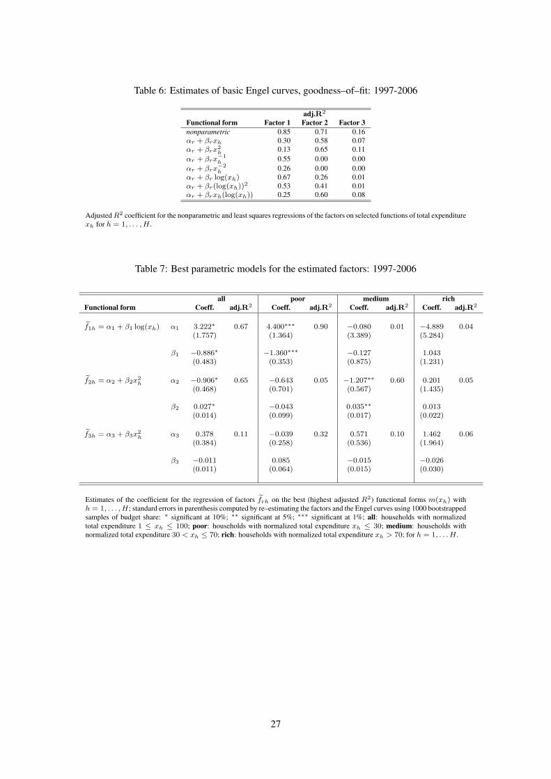
Table 6: Estimates of basic Engel curves, goodness–of–fit: 1997-2006

adj.R2

Functional form Factor 1 Factor 2 Factor 3

nonparametric 0.85 0.71 0.16

αr + βrxh 0.30 0.58 0.07

αr + βrx2h

0.13 0.65 0.11

αr + βrx−1h

0.55 0.00 0.00

αr + βrx−2h

0.26 0.00 0.00

αr + βr log(xh) 0.67 0.26 0.01

αr + βr(log(xh))2 0.53 0.41 0.01

αr + βrxh(log(xh)) 0.25 0.60 0.08

Adjusted R2 coefficient for the nonparametric and least squares regressions of the factors on selected functions of total expenditure

xh for h = 1, . . . , H .

Table 7: Best parametric models for the estimated factors: 1997-2006

all poor medium rich

Functional form Coeff. adj.R2 Coeff. adj.R2 Coeff. adj.R2 Coeff. adj.R2

f1h = α1 + β1 log(xh) α1 3.222∗ 0.67 4.400∗∗∗ 0.90 −0.080 0.01 −4.889 0.04(1.757) (1.364) (3.389) (5.284)

β1 −0.886∗ −1.360∗∗∗ −0.127 1.043(0.483) (0.353) (0.875) (1.231)

f2h = α2 + β2x2h

α2 −0.906∗ 0.65 −0.643 0.05 −1.207∗∗ 0.60 0.201 0.05(0.468) (0.701) (0.567) (1.435)

β2 0.027∗ −0.043 0.035∗∗ 0.013(0.014) (0.099) (0.017) (0.022)

f3h = α3 + β3x2h

α3 0.378 0.11 −0.039 0.32 0.571 0.10 1.462 0.06(0.384) (0.258) (0.536) (1.964)

β3 −0.011 0.085 −0.015 −0.026(0.011) (0.064) (0.015) (0.030)

Estimates of the coefficient for the regression of factors frh on the best (highest adjusted R2) functional forms m(xh) with

h = 1, . . . , H; standard errors in parenthesis computed by re–estimating the factors and the Engel curves using 1000 bootstrapped

samples of budget share: ∗ significant at 10%; ∗∗ significant at 5%; ∗∗∗ significant at 1%; all: households with normalized

total expenditure 1 ≤ xh ≤ 100; poor: households with normalized total expenditure xh ≤ 30; medium: households with

normalized total expenditure 30 < xh ≤ 70; rich: households with normalized total expenditure xh > 70; for h = 1, . . . H .

27

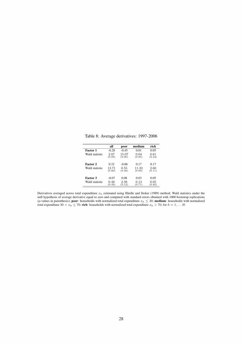
Table 8: Average derivatives: 1997-2006

all poor medium rich

Factor 1 -0.28 -0.45 0.01 0.05

Wald statistic 2.87(0.09)

15.07(0.00)

0.04(0.85)

0.61(0.44)

Factor 2 0.32 -0.06 0.17 0.17

Wald statistic 12.71(0.00)

0.55(0.46)

11.33(0.00)

2.60(0.11)

Factor 3 -0.07 0.08 0.03 0.05

Wald statistic 0.48(0.49)

2.38(0.12)

0.13(0.71)

0.05(0.82)

Derivatives averaged across total expenditure xh estimated using Hardle and Stoker (1989) method; Wald statistics under the

null hypothesis of average derivative equal to zero and computed with standard errors obtained with 1000 bootstrap replications

(p-values in parenthesis); poor: households with normalized total expenditure xh ≤ 30; medium: households with normalized

total expenditure 30 < xh ≤ 70; rich: households with normalized total expenditure xh > 70; for h = 1, . . . H .

28

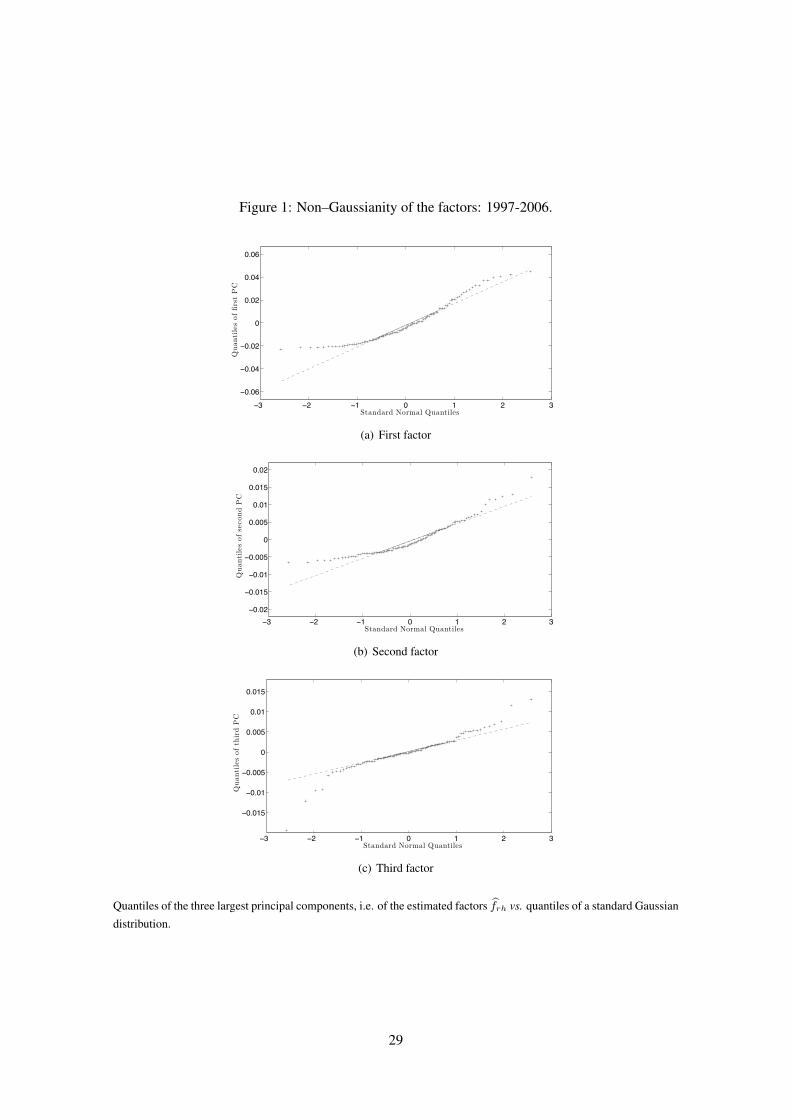
Figure 1: Non–Gaussianity of the factors: 1997-2006.

(! (∀ (# ∃ # ∀ !

(∃%∃&

(∃%∃∋

(∃%∃∀

∃

∃%∃∀

∃%∃∋

∃%∃&

Standard Normal Quantiles

QuantilesoffirstPC

(a) First factor

(! (∀ (# ∃ # ∀ !

(∃%∃∀

(∃%∃#&

(∃%∃#

(∃%∃∃&

∃

∃%∃∃&

∃%∃#

∃%∃#&

∃%∃∀

Standard Normal Quantiles

QuantilesofsecondPC

(b) Second factor

(! (∀ (# ∃ # ∀ !

(∃%∃#&

(∃%∃#

(∃%∃∃&

∃

∃%∃∃&

∃%∃#

∃%∃#&

Standard Normal Quantiles

Quantilesofth

irdPC

(c) Third factor

Quantiles of the three largest principal components, i.e. of the estimated factors frh vs. quantiles of a standard Gaussian

distribution.

29

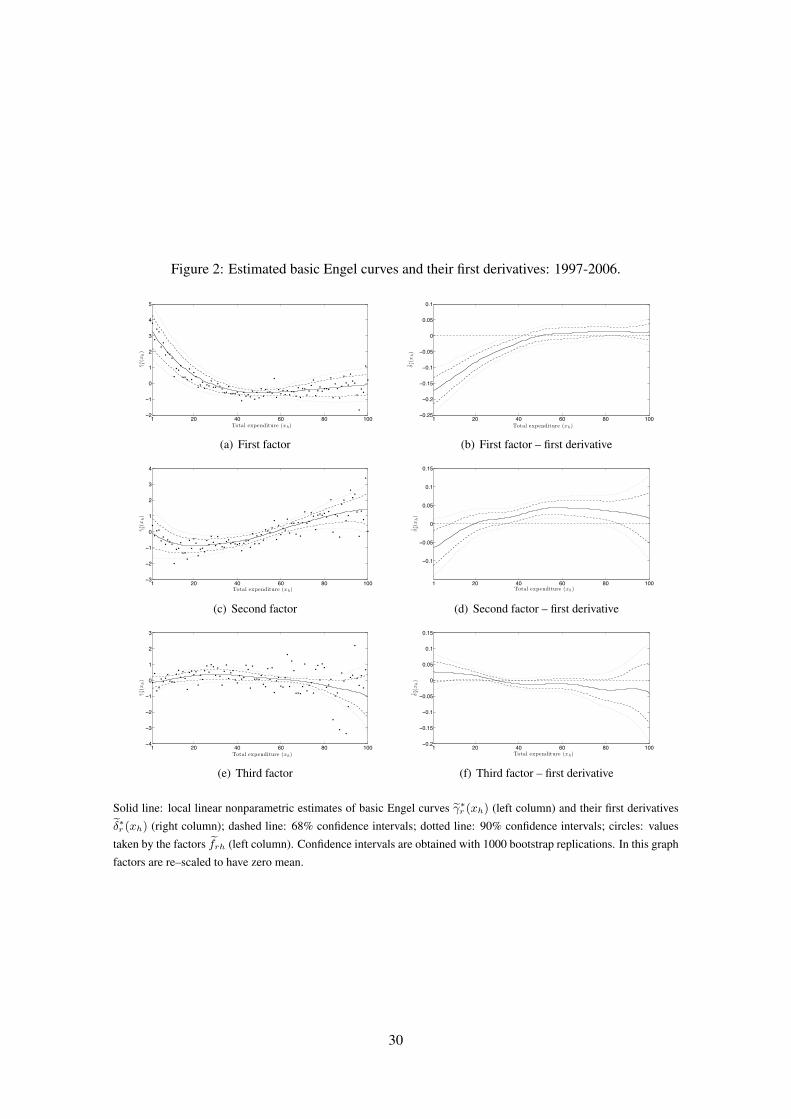
Figure 2: Estimated basic Engel curves and their first derivatives: 1997-2006.

! ∀# ∃# %# &# !##(∀

(!

#

!

∀

∋

∃

(

Total expenditure (xh)

γ∗ 1(x

h)

(a) First factor

! ∀# ∃# %# &# !##(#∋∀(

(#∋∀

(#∋!(

(#∋!

(#∋#(

#

#∋#(

#∋!

Total expenditure (xh)

δ∗ 1(x

h)

(b) First factor – first derivative

! ∀# ∃# %# &# !##(∋

(∀

(!

#

!

∀

∋

∃

Total expenditure (xh)

γ∗ 2(x

h)

(c) Second factor

! ∀# ∃# %# &# !##

(#∋!

(#∋#(

#

#∋#(

#∋!

#∋!(

Total expenditure (xh)

δ∗ 2(x

h)

(d) Second factor – first derivative

! ∀# ∃# %# &# !##(∃

(∋

(∀

(!

#

!

∀

∋

Total expenditure (xh)

γ∗ 3(x

h)

(e) Third factor

! ∀# ∃# %# &# !##(#∋∀

(#∋!(

(#∋!

(#∋#(

#

#∋#(

#∋!

#∋!(

Total expenditure (xh)

δ∗ 3(x

h)

(f) Third factor – first derivative

Solid line: local linear nonparametric estimates of basic Engel curves γ∗

r (xh) (left column) and their first derivatives

δ∗r (xh) (right column); dashed line: 68% confidence intervals; dotted line: 90% confidence intervals; circles: values

taken by the factors frh (left column). Confidence intervals are obtained with 1000 bootstrap replications. In this graph

factors are re–scaled to have zero mean.

30

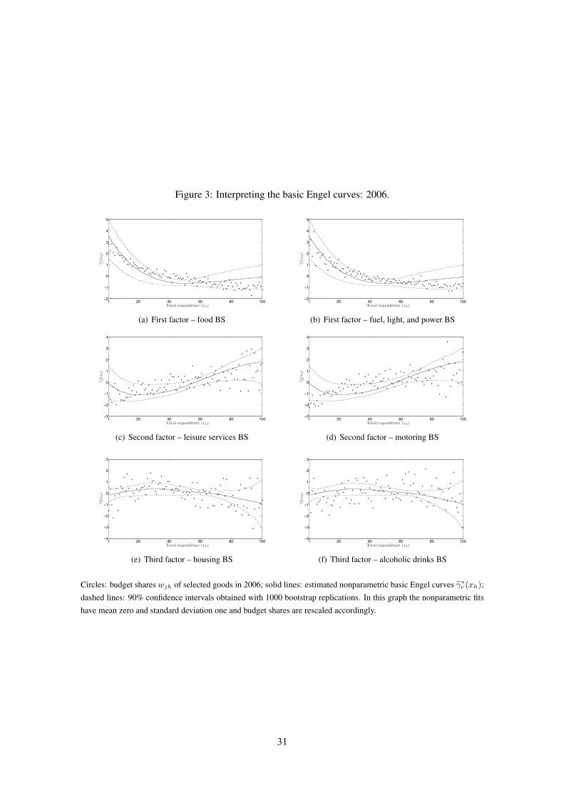
Figure 3: Interpreting the basic Engel curves: 2006.

! ∀# ∃# %# &# !##(∀

(!

#

!

∀

∋

∃

(

Total expenditure (xh)

γ∗ 1(x

h)

(a) First factor – food BS

! ∀# ∃# %# &# !##(∀

(!

#

!

∀

∋

∃

(

Total expenditure (xh)

γ∗ 1(x

h)

(b) First factor – fuel, light, and power BS

! ∀# ∃# %# &# !##(∋

(∀

(!

#

!

∀

∋

∃

Total expenditure (xh)

γ∗ 2(x

h)

(c) Second factor – leisure services BS

! ∀# ∃# %# &# !##(∋

(∀

(!

#

!

∀

∋

∃

Total expenditure (xh)

γ∗ 2(x

h)

(d) Second factor – motoring BS

! ∀# ∃# %# &# !##(∃

(∋

(∀

(!

#

!

∀

∋

Total expenditure (xh)

γ∗ 3(x

h)

(e) Third factor – housing BS

! ∀# ∃# %# &# !##(∃

(∋

(∀

(!

#

!

∀

∋

Total expenditure (xh)

γ∗ 3(x

h)

(f) Third factor – alcoholic drinks BS

Circles: budget shares wjh of selected goods in 2006; solid lines: estimated nonparametric basic Engel curves γ∗

r (xh);

dashed lines: 90% confidence intervals obtained with 1000 bootstrap replications. In this graph the nonparametric fits

have mean zero and standard deviation one and budget shares are rescaled accordingly.

31

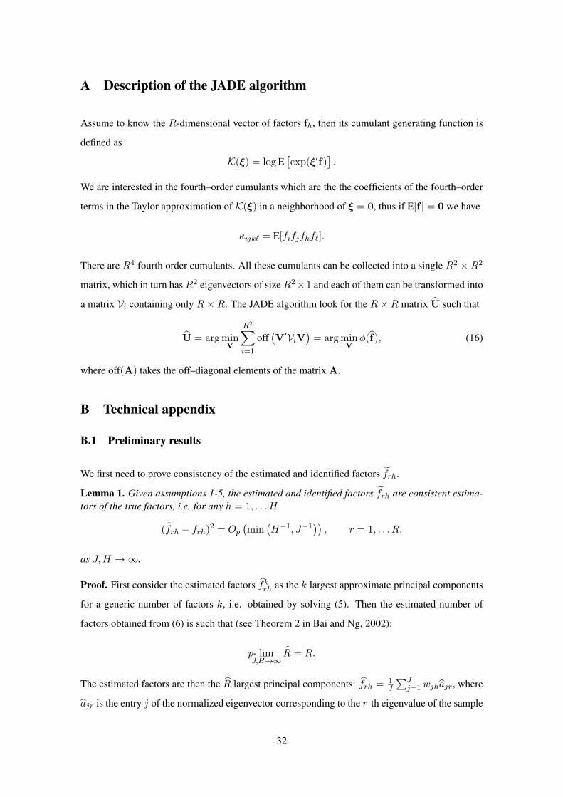
A Description of the JADE algorithm

Assume to know the R-dimensional vector of factors fh, then its cumulant generating function is

defined as

K(ξ) = logE[exp(ξ′f)

].

We are interested in the fourth–order cumulants which are the the coefficients of the fourth–order

terms in the Taylor approximation of K(ξ) in a neighborhood of ξ = 0, thus if E[f ] = 0 we have

κijkℓ = E[fifjfhfℓ].

There are R4 fourth order cumulants. All these cumulants can be collected into a single R2 ×R2

matrix, which in turn hasR2 eigenvectors of sizeR2×1 and each of them can be transformed into

a matrix Vi containing only R×R. The JADE algorithm look for the R×R matrix U such that

U = argminV

R2∑

i=1

off(V′ViV

)= argmin

V

φ(f), (16)

where off(A) takes the off–diagonal elements of the matrix A.

B Technical appendix

B.1 Preliminary results

We first need to prove consistency of the estimated and identified factors frh.

Lemma 1. Given assumptions 1-5, the estimated and identified factors frh are consistent estima-

tors of the true factors, i.e. for any h = 1, . . . H

(frh − frh)2 = Op

(min

(H−1, J−1

)), r = 1, . . . R,

as J,H → ∞.

Proof. First consider the estimated factors fkrh as the k largest approximate principal components

for a generic number of factors k, i.e. obtained by solving (5). Then the estimated number of

factors obtained from (6) is such that (see Theorem 2 in Bai and Ng, 2002):

p- limJ,H→∞

R = R.

The estimated factors are then the R largest principal components: frh = 1J

∑Jj=1wjhajr, where

ajr is the entry j of the normalized eigenvector corresponding to the r-th eigenvalue of the sample

32

covariance matrix of wh. From a corollary of Theorem 1 in Bai and Ng (2002) we have

∣∣∣∣∣∣fh −Ufh

∣∣∣∣∣∣2= Op

(min

(J−1, H−1

)), for any h = 1, . . . , H, (17)

where U is a matrix of rank r.

If we assume statistical independence among the R components of the factors fh (see assump-

tions 4 and 5) then U is uniquely identifiable. For example from JADE we obtain an estimate U

such that U′fh has R statistically independent components. Moreover, since from (16) and the

fact that sample cumulants are continuous function of the factors, and by virtue of (17), we have

(φ(f)− φ(Uf))2 = Op

(min

(J−1, H−1

)),

which implies ∣∣∣∣∣∣U

f− UUf

∣∣∣∣∣∣2= Op

(min

(J−1, H−1

)). (18)

where Uf

is the maximizer of (16) when using the fourth–order cumulants of f and analogously

we define UUf .

Since for any vector x, JADE determines Ux in order to make the components of the vector

U′xx statistically independent, then U′

UfUfh has statistically independent components. Given that

the ICA problem has a unique solution up to a sign, a scale, and a permutation, and given that by

assumption fh has already independent components, then we must have U′Uf

U = Ir. Indeed we

can fix the sign, scale, and permutation indeterminacy by adding assumptions on the true factors

as described in the main text.

By multiplying both terms in (17) by Uf

we have

∣∣∣∣∣∣U

ffh − U

fUfh

∣∣∣∣∣∣2≤∣∣∣∣∣∣U

ffh − UUfUfh

∣∣∣∣∣∣2+∣∣∣∣∣∣UUfUfh − U

fUfh

∣∣∣∣∣∣2, h = 1, . . . , H,

From (18) we have that the second term on the right–hand–side is Op

(min

(J−1, H−1

)). More-

over, from (17) also the term on the left–hand–side is Op

(min

(J−1, H−1

)), therefore also the

first term on the right–hand–side must be Op

(min

(J−1, H−1

)). If we define fh = U

ffh and

recalling that U′Uf

U = Ir, this latter term becomes

∣∣∣∣∣∣U

ffh − UUfUfh

∣∣∣∣∣∣2=∣∣∣∣∣∣fh − fh

∣∣∣∣∣∣2= Op

(min

(J−1, H−1

)), for any h = 1, . . . , H,

or equivalently

∣∣∣frh − frh

∣∣∣2= Op

(min

(J−1, H−1

)), for any h = 1, . . . , H, r = 1, . . . R, (19)

33

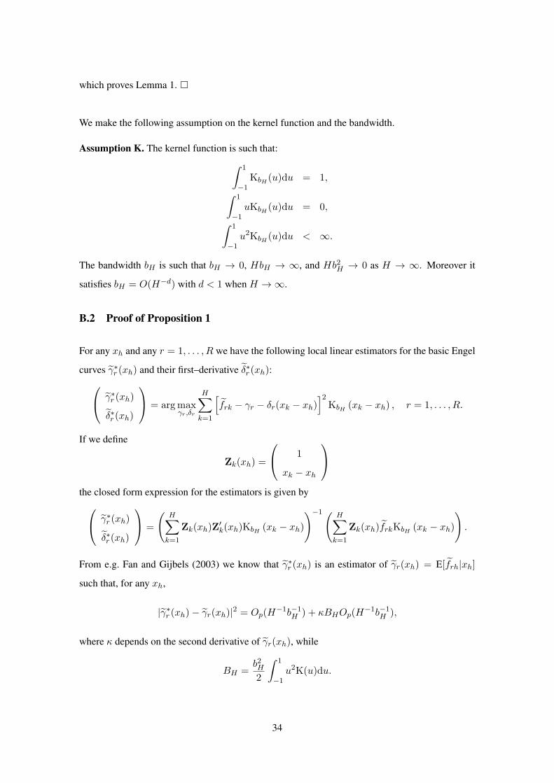
which proves Lemma 1. �

We make the following assumption on the kernel function and the bandwidth.

Assumption K. The kernel function is such that:

∫ 1

−1KbH (u)du = 1,

∫ 1

−1uKbH (u)du = 0,

∫ 1

−1u2KbH (u)du < ∞.

The bandwidth bH is such that bH → 0, HbH → ∞, and Hb2H → 0 as H → ∞. Moreover it

satisfies bH = O(H−d) with d < 1 when H → ∞.

B.2 Proof of Proposition 1

For any xh and any r = 1, . . . , R we have the following local linear estimators for the basic Engel

curves γ∗r (xh) and their first–derivative δ∗r (xh):

γ∗r (xh)

δ∗r (xh)

= argmax

γr,δr

H∑

k=1

[frk − γr − δr(xk − xh)

]2KbH (xk − xh) , r = 1, . . . , R.

If we define

Zk(xh) =

1

xk − xh

the closed form expression for the estimators is given by

γ∗r (xh)

δ∗r (xh)

=

(H∑

k=1

Zk(xh)Z′k(xh)KbH (xk − xh)

)−1( H∑

k=1

Zk(xh)frkKbH (xk − xh)

).

From e.g. Fan and Gijbels (2003) we know that γ∗r (xh) is an estimator of γr(xh) = E[frh|xh]

such that, for any xh,

|γ∗r (xh)− γr(xh)|2 = Op(H−1b−1

H ) + κBHOp(H−1b−1

H ),

where κ depends on the second derivative of γr(xh), while

BH =b2H2

∫ 1

−1u2K(u)du.

34

Therefore,

|γ∗r (xh)− γr(xh)|2 = Op(H−1b−1

H ) +Op(b2HH

−1b−1H ). (20)

Now consider the following decomposition, which holds for any r = 1, . . . R and any h =

1, . . . H

|γ∗r (xh)− gr(xh)|2 = |γ∗r (xh)− γr(xh) + γr(xh)− gr(xh)|2 ≤

≤ |γ∗r (xh)− γr(xh)|2 + |γr(xh)− gr(xh)|2.

Given (20), the first term in the last inequality is Op(H−1b−1

H ) + Op(bHH−1), while the second

term can be written as

∣∣∣E[frh|xh

]− E

[frh|xh

]∣∣∣2=∣∣∣E[(frh − frh)|xh

]∣∣∣2≤ E

[∣∣∣frh − frh

∣∣∣2|xh]= Op

(min

(J−1, H−1

)).

where the last equality is given by Lemma 1. Therefore,

|γ∗r (xh)− gr(xh)|2 ≤ Op(H−1b−1

H ) +Op(bHH−1) +Op

(min

(J−1, H−1

)). (21)

Since when H → ∞ assumption K implies bH → 0, HbH → ∞, and bHH−1 → 0, we have

p- limJ,H→∞

|γ∗r (xh)− gr(xh)|2 = 0,

which proves Proposition 1, the rate of convergence being given by (21). An analogous argument

allows us to prove consistency of the first derivative, i.e.

p- limJ,H→∞

|δ∗r (xh)− g′r(xh)|2 = 0.

�

B.3 Proof of Proposition 2

The proof is based on the same arguments as the proof of Proposition 1. Consider the equation

frh = αr + βrm(xh) + zrh, r = 1, . . . , R; h = 1, . . . , H, (22)

then define

X = (1H ,m(x)), θr =

αr

βr

, r = 1, . . . , R,

35

where 1H is an H-dimensional column vector of ones and x = (x1 . . . xH)′. The least squares

estimator of (22)

θ∗r = (X ′X )−1X ′fr,

is such that (see e.g. Gourieroux et al., 1984)

p-limH→∞

|θ∗r − θr| = 0, r = 1, . . . , R, (23)

with rate H−1/2. Now consider, for any r = 1, . . . , R,

|θ∗r − θr| = |θ∗

r − θr + θr − θr| ≤ |θ∗r − θr|+ |θr − θr| (24)

the first term on the right–hand–side is Op(H−1/2). If we multiply the second term by X we have

X|θr − θr| = |X θr −Xθr| = E[fr − fr|X

]= Op

(min

(J−1/2, H−1/2

)), (25)

by Lemma 1. By combining (23), (24), and (25) we get the required result. �

36

C Data description

Disaggregation at 4-digits level of the 13 expenditure categories considered.

.01 HOUSING: ACCOMMODATION COSTS, REPAIRS AND IMPROVEMENTS

.01.01 Rent, mortgages, council tax, water, home insurance

.01.02 Purchase of main dwelling and caravan/mobile home

.01.03 Capital improvements and maintenance by contractor: Main and second dwelling

.01.04 D-I-Y improvements: Main and second dwelling

.01.05 Purchase of materials, fittings, tools-home maintenance

.01.06 Second dwelling purchase and running costs

.02 FUEL, LIGHT AND POWER

.02.01 Gas expenditure

.02.02 Electricity expenditure

.02.03 Coal and other fuel

.03 FOOD

.03.01 Cereals and cereal products

.03.02 Milk and milk products

.03.03 Eggs

.03.04 Fats and oils

.03.05 Meat and meat products

.03.06 Fish, shellfish and products

.03.07 Vegetables and pulses

.03.08 Fruit and nuts

.03.09 Sugar, preserves and confectionery

.03.10 Beverages (non-alcoholic)

.03.11 Miscellaneous foods

.03.12 Take away meals eaten at home + meals on wheels

.03.13 Food bought and consumed at work, school

.03.15 Food from other outlets not eaten at home

.03.16 Meals/snacks not eaten at home (child)

.03.17 Food stamps

.04 ALCOHOLIC DRINKS

.04.01 Alcohol Bought Off Licensed Premises

.04.02 Alcohol bought and consumed on licensed premises

.05 TOBACCO

.06 CLOTHING AND FOOTWEAR

.06.01 Outerwear

.06.02 Underwear and hosiery

.06.03 Clothing accessories

.06.04 Footwear

.06.05 Haberdashery and clothing materials

.07 HOUSEHOLD GOODS

.07.01 Furniture and furnishings

.07.02 Electrical and gas appliances and consumables

.07.03 Non-electrical kitchenware, hardware, decorative goods

.07.04 Cleaning materials

.07.05 Toilet paper

.07.06 Pet expenditure

.07.07 Garden expenditure

.07.08 Household goods miscellaneous

.08 DOMESTIC AND PAID SERVICES, POSTAGE, PHONE, SUBS (HOUSEHOLD SERVICES)

.08.01 Childcare, laundry, cleaning, repairs-personal goods

.08.02 Postage and telephones

.08.03 Subscriptions

.08.04 Legal, financial, professional fees and costs

.08.05 Other services contracted or hired

.09 PERSONAL GOODS AND SERVICES

.09.01 Cosmetics/toilet requisites

.09.02 Personal effects and travel goods

.09.03 Baby goods

.09.04 Medicines and medical goods

.09.05 Spectacles

.09.06 Hairdressing, beauty treatments and wigs etc.

.09.07 Other personal goods

37

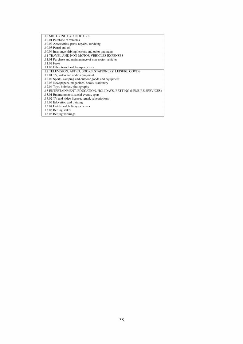
.10 MOTORING EXPENDITURE

.10.01 Purchase of vehicles

.10.02 Accessories, parts, repairs, servicing

.10.03 Petrol and oil

.10.04 Insurance, driving lessons and other payments

.11 TRAVEL AND NON-MOTOR VEHICLES EXPENSES

.11.01 Purchase and maintenance of non-motor vehicles

.11.02 Fares

.11.03 Other travel and transport costs

.12 TELEVISION, AUDIO, BOOKS, STATIONERY, LEISURE GOODS

.12.01 TV, video and audio equipment

.12.02 Sports, camping and outdoor goods and equipment

.12.03 Newspapers, magazines, books, stationery

.12.04 Toys, hobbies, photography

.13 ENTERTAINMENT, EDUCATION, HOLIDAYS, BETTING (LEISURE SERVICES)

.13.01 Entertainments, social events, sport

.13.02 TV and video licence, rental, subscriptions

.13.03 Education and training

.13.04 Hotels and holiday expenses

.13.05 Betting stakes

.13.06 Betting winnings

38