Working Paper 02-32 Economics Series 13 February 2003

Departamento de EconomíaUniversidad Carlos III de Madrid

Calle Madrid, 12628903 Getafe (Spain)

Fax (34) 91 624 98 75

SPILLOVERS IN PRODUCT AND PROCESS INNOVATION: EVIDENCE FROM MANUFACTURING FIRMS *

Carmine Ornaghi1

Abstract This paper proposes a new empirical approach to assess the impact of knowledge

spillovers on firms' productivity and demand. I consider a model where process innovations spillovers to other firms raise firms relative efficiency and technological diffusion of product innovations enhances firms' demand. By modelling knowledge capital as a function of own investment in R\&D and spillovers, I can compare the impact of these two complementary sources of knowledge on both the supply and the demand side. The results obtained confirm the findings already highlighted by previous empirical studies that technological externalities affect significantly firms' productivity growth. The new result obtained is that technological diffusion of product innovations is larger than the one deriving from process innovations, both in magnitude and pervasiveness.

Keywords: Innovation; Knowledge capital; Spillovers. JEL Classification: L61, O30.

1 Departamento de Economía, Universidad Carlos III de Madrid. E.mail: carmine@eco.uc3m.es * I wish to thank Jordi Jaumandreu and Pedro Marin for many helpful discussions and suggestions. I benefit from comments from Bronwyn Hall, Matilde Machado, Georges Siotis and participants in seminars at Universidad Carlos III de Madrid and University of California at Berkeley.

1 Introduction

Since the seminal paper of Griliches (1979) on the productivity effect ofR&D, several economists have investigated the relationship between firms’innovation and productivity growth. The first studies aimed at assessing theimportance of research in explaining productivity improvements relied on in-serting another type of capital, computed from data on R&D expenditure, tothe list of inputs entering the production function. But economists have soonrealized that this type of capital (generally defined knowledge capital) doesnot depend only on firms own investments in R&D. The non-rival characterof knowledge implies that a firm may learn from other firms’ innovations,whenever the technological contents of their R&D activities are not success-fully confined inside their walls. Thus, the firm’s productivity also dependson the pool of general knowledge it has access to. This is what is known astechnological externalities or spillovers. By including a proxy for this variablein the firm production function, it is possible to determine whether spilloversplay an important role in generating productivity growth.1 The economy, asa whole, would be enriched with such a positive externality since it representsa source of increasing social returns.

The common feature of all these studies is that technological innovationis assumed to be process oriented: the knowledge capital acquired by a firmimproves the mechanism by which input is transformed into output. But thisapproach ignores another important dimension of innovation: improvementsin the quality of existing products and the introduction of new goods. Study-ing the impact of spillovers only on the supply or productivity side can showonly part of the picture. A firm that enhances the quality of its products bylearning the technological innovations introduced by competitors is receivinga positive externality that can be estimated only shifting the attention tothe demand or consumption side.2 Moreover, consider that the channels of

1There is a large literature that deals with the empirical estimation of spillovers in theframework of productivity analysis. Griliches (1992) and Nadiri (1993) offer extensive sur-veys of the main contributions. Although the magnitude of spillover seems to vary largelybetween industries and countries, the relevance of technology spillovers is not questioned.See Los and Verspagen (2000) for a recent study.

2Mansfield, Rapport, Romeo and Wagner (1977) conduct a number of case-studies toestimate social and private rate of return from investments in product and process in-novation. Moreover, several papers have used this distinction to get interesting insights

2

technology spillovers are hardly the same. Imitation of a product innovationcan be simply achieved through reverse engineering while diffusion of processinnovation may require more sophisticated channels, such as industrial espi-onage or recruitment of engineers and experts of rival firms. Therefore, themagnitude and pervasiveness of spillovers for product and process R&D arelikely to be different. Although both of them can possibly lead to an increasein the output produced by the firm, the forces behind this output expansionare quite different and deserve a separate analysis.

This paper proposes an original empirical approach to the problem ofassessing the impact of knowledge spillovers on firms’ productivity and de-mand. I consider a model where process innovations spillovers to other firmsraise firms relative efficiency and technological diffusion of product innova-tions enhances firms’ demand. To the best of my knowledge, there are nosimilar studies in the empirical literature on spillovers. By modelling knowl-edge capital as a function of own investment in R&D and spillovers, I cancompare the impact of these two complementary sources of knowledge onboth the supply and the demand side. The results obtained confirm thefindings already highlighted by previous empirical studies that technologicalexternalities affect significantly firms’ productivity growth. The new insightpresented is that the magnitude and pervasiveness of spillovers from productinnovation are larger than those coming from process innovation.3

The data base used in this paper reports detailed information on firms’individual input, R&D expenditure, types of innovation achieved as well asobservations on output price changes and other demand-related variables,which is a rather unusual feature. This allows me not only to specify thericher framework explained above but also to introduce new features in defin-ing the knowledge capital that can partially overcome the problems usuallyfound in the empirical literature. By employing the available information ontype and timing of innovations, I can model the transformation of research

in related areas. Mansfield (1983), for example, surveys the major product and processinnovations in the chemical, drug, petroleum, and steel industries to shed some light onthe effects of technological change on market structure. Levin and Reiss (1988) definea theoretical framework to analyse the tradeoffs that firms face between imperfectly ap-propriable product and process innovation, when underlying technological opportunitiesdiffer.

3A similar framework is used in Garcia, Jaumandreu and Rodriguez (2002) to studythe elasticity of employment with respect to innovations.

3

into productivity gains and product quality improvements. The resultingmeasure of internal R&D can then be considered a better proxy for innova-tion output. As discussed below, this refinement leads to a relevant increasein the point estimate of R&D capital coefficients for both the productionfunction and the demand equation. As far as the spillover variable is con-cerned, I generalize previous characterisations of the potential spillover pool,constructing different measures of proximity according to basic firm’s charac-teristics, such as the number of employees or the localization. This approachcan be considered an alternative to the one defined by Jaffe (1986) usingfirm data on the distribution of patents,4 as it allows to refine the measureof spillovers without relying on detailed patenting data (that are generallynot available). The results obtained suggest that size is a main determinantof the magnitude and extent of technology dissemination.

The nature of this study requires the analysis of a large sample of mar-kets. To the extent that technological innovations can be applied to severalmanufacturing sectors, a cross-sectional approach seems an objective wayto get useful stylized facts on the magnitude of spillovers in industrializedcountries. This paper is based on an unbalanced panel data of Spanish man-ufacturing firms that includes more than 2,000 entities during the period1990-1999. The surveyed sample is made up of firms performing and notperforming R&D activities respecting the population proportions.

The article is organized as follows. Section 2 provides the econometricframework used to estimate the magnitude of spillovers for the productionfunction and the demand equation. Section 3 presents the data set and thespecification of the knowledge variables. Empirical results are summarizedin Section 4. Some final comments are presented in the concluding section.

4Using data on the distribution of patents, Jaffe (1986) first defines the “technologicalposition” of a firm’s research program and then he constructs a measure of proximityamong firms according to the correlation of their “technological position vector”. Heassumes that the closer are two firms in their research program, the higher is the fractionof R&D capital that can leak out.

4

2 Modelling Spillovers in Product and ProcessR&D

In this section, I discuss the details of the econometric framework that is usedto estimate the impact of spillovers on production and demand. Assume thatthe output of firm i in period t, Y pit , is produced from three “conventional”inputs, labour Lit, materials Mit and physical capital Cit and also dependson a technological parameter A, which in turn is a function of the industryj’s specific rate of disembodied technical change, λjt, the individual researcheffort of the firm, Rit, and the knowledge spillovers, Sit. In order to controlfor short term adjustments associated with the business cycle, the degreeof capacity utilization, U, is added as a further explanatory variable in theproduction function..5 According to this explanation, the firm productionfunction takes the form:

Y pit = A (λjt, Rit, Sit)F (Lit,Mit, Cit, Uit) (1)

Now assume that the demand equation can be written as:

Y git = D(Pit, ADit, Rit, Sit, Z−it) (2)

where Y git is the quantity demanded, Pit refers to price, and ADit standsfor advertising. Again, the knowledge capital of a firm is made up of theindividual research effort Rit and the spillover pool Sit. The latter variable ismeant to measure the effect on demand of any product quality improvementsachieved by learning the technological innovation first introduced by a com-petitor. Finally, Z−i is a vector of prices, knowledge capital and advertisingfor rivals.

Equation (2) adapts to a model of vertical differentiation where bothknowledge capital and advertising will affect the demand through an im-

5The production function is defined as a relation between flow of output and inputs.While annual price and quantity data are generally available for labour and materials,physical capital C is usually computed as a stock using the perpetual inventory method.As noted by Hulten (2000), this approach is valid only as long a flow of services from capitalare proportional to the stock. But proportionality is not always a realistic assumption,in particular during period of low demand characterized by low capital utilization. Thistopic is investigated in a companion paper, Ornaghi (2002).

5

provement of real and perceived product quality, respectively.6 Notice thatthe demand enhancing effect of knowledge capital can materialise via twodifferent mechanisms: a market expansion effect and a business stealing ef-fect. In the first case the introduction of new products, by attracting newconsumers to the market, can benefit the pioneer firm and all the firms thatsuccessfully adopt the innovation without necessarily affecting less innovativefirms. In a context where market expansion effects are minimum comparedto business stealing effect, some firms will expand their activities in detri-ment of their competitors. In both cases, it is likely that only some firmswill be able to reproduce the innovation achieved by competitors, dependingon their characteristics. Results presented in Section 4 suggest that size is amain determinant of a firm’s capacity of learning from rivals.

The possible positive impact on a firm demand schedule of other firms’investments in product improvements is likely to depend on the way marketsare classified. If we define an industry broadly enough to consider verticalrelations or complementary products, then it is evident that a firm’s prod-uct innovation may have a positive effect on other firms’ demand.7 It isthen an interesting exercise to assess whether any difference in the magni-tude between spillovers for product and process R&D tends to change withalternative classification of the industries making up the manufacturing sec-tor. The results obtained suggest that technological externalities associatedto product innovations have a broader impact: firms can take advantage ofproduct improvements introduced by firms in not strictly related markets.On the other hand, spillovers from process innovations are limited to nar-rowly defined industries.

Following the approach used by Klette (1996 and 1999), the productionfunction can be expressed in terms of logarithmic deviations from a refer-ence input-output vector (e.g.,Y pot, Lot,Mot, ..). This point of reference canbe thought of as the representative firm that each firm within an industryhas to compete with. In the empirical application, I have characterised this

6The demand equation might depend on other elements, such as brand image or cus-tumers’ loyalty. As explained below, estimation in first-differences are not affected as longas these omitted elements are constant over time.

7Consider the case of the computer industry. Usually the introduction of a new dataprocessor has a demand expanding effect for producer of computer equipment and software.Moreover, this can expand the sales of complementary products such as scanners, printersand multimedia apparatus.

6

reference point as the average values of output and inputs within the 3-digitCNAE code industry in each year.8 The use of a year-specific industry meanvalue eliminates the technical change, λj, from specification (1). It followsthat there is no need to introduce time-dummies in the estimation. This nor-malisation has the additional advantage of refining the model from omittedfactors that are common to all the firms within a (3-digit CNAE) indus-try, thus attenuating the problem of great heterogeneity associated to cross-industry studies. In the same way, the demand equation can be expressedusing a log-linear expansion around the reference firm (e.g.,Y dot, Pot, ADot, ..).Although estimation of the demand relationship would require complete in-formation on rivals’ prices and other relevant variables, this transformationallows us to consider the effect of an average change in rival’s prices, knowl-edge capital and advertising expenditure on the quantity demanded.9

Rewriting equation (1) and (2), in terms of logarithmic deviations fromthe representative firm, we obtain:

ypit = α1 lit + α2mit + α3cit + α4uit + α5rit + α6sit + εit (3)

and

ygit = β1bpit + β2cadit + β3brit + β4sit + ζ it (4)

where lowercase letters with a hat stand for logarithm deviations from thepoint of reference of their upper-case counterparts, e.g. ypit=ln(Y

pit/Y

pot); εit is

the random error term for the production function, representing the effect ofefficiency differences, functional form discrepancies and measurement errorswhile ζ it is the error component capturing stochastic shocks to the demand.

There are two relevant econometric issues that have to be carefully con-sidered at this point. Firstly, one of the most important components ofε in the production function is likely to be due to firm-specific factors ofproduction, such as entrepreneurial ability, that are not observable. Thiscomponent determines productivity differences between firms that tend to

8The CNAE classification embraces about 120 different manufacturing sectors. Thisclassification is similar to the 3-digit ISIC in terms of market definition.

9Normalizing the demand equation with respect to the reference firm, we can alsoeliminate any market dynamism (e.g. market expansion or recession) that is common toall the firms in the industry. Kettle (1996) uses a similar approach to model the demandequation.

7

be rather persistent over time. We can consequently decompose the errorterm as:

εit = µi + vit (5)

where µi is the just mentioned fixed-effect that account for the perma-nent heterogeneity across firms whereas v includes temporary productivityshocks and measurement errors. To the extent that µi affects the current in-put choice decisions, the assumption of no correlation between the includedregressors and the disturbance term does not hold and this prevents us fromusing Ordinary Least Square (OLS) estimation. The persistency of high au-tocorrelation of the errors in the OLS estimation (in levels) suggests thatunobserved heterogeneity is a relevant issue that must not be undervalued.10

Therefore, we estimate equation (3) in “first differences” in order to eliminatethe term µi from the specification of the production function:

ypit = α1lit + α2mit + α3cit + α4uit + α5rit + α6sit + vit (P)

where lower case letters with tilde represent log differences of the variablesnormalized with respect to the representative firm, that is ypit=ln(Y

pit/Y

pot)−

ln(Y pit−1/Ypot−1).

In the same way, there are some (omitted) elements, such as the brandimage or the consumers’ loyalty, buried in the residual of the demand equa-tion that are presumably constant over time. By taking first differences toeliminate these omitted variables, we obtain the estimating equation:

ygit = β1epit + β2fadit + β3erit + β4esit + ϑit (G)

Secondly, consistent estimation of equation (P) and (G) by OLS requirespredeterminacy of the regressors. As far as the production function is con-cerned, whenever a productivity shock is anticipated before the optimal quan-tity of inputs is chosen, disturbances vit are transmitted to the decision equa-tion of the inputs. This means that there is a positive correlation betweenthe right-hand variables and the error term, thereby invalidating the use ofOLS estimation. This delicate econometric issue is known in the literature10This evidence is confirmed by the results of the Hausman test, which rejects the null

hypothesis that the “random effect” estimates are not statistically different from the onebased on the “fixed effect” model. See Greene (1997) for further details.

8

as the simultaneity problem.11 Among the three standard input variablesof equation (P), labour, L, is the one more likely to be correlated with theerror term. Besides, using the Sargan difference test, the null hypothesisof exogeneity of the capacity utilization term is rejected. We then use pastvalues of labour and capacity utilization to instrument these two endogenousvariables. A similar issue needs to be considered for the demand relation-ship: the simultaneity between price and quantity demanded. As shown ina standard downward-sloping demand curve, when the price increases, thequantity demanded falls. At the same time, quantity affects the price thoughtthe supply curve whenever the latter is not horizontal (infinite price elastici-ties). This implies that an unobservable exogenous demand shock can affectnot only purchases but also prices. The latter are then endogenous variablesand OLS regression does not give consistent estimation of the parametersdefined in equation (G). The use of panel data provides a solution to thisproblem since we can use lags of this endogenous variable as instruments. Ishall come back on this point in Section 4

3 Data and Variables

The data used in this study are retrieved from the Encuesta sobre Estrate-gias Empresariales, ESEE, (Business Strategy Survey) an unbalanced panelsample of Spanish manufacturing firms published by the Fundación EmpresaPública covering the period 1990-1999. The raw dataset consists of 3,151firms for a total number of 18,680 observations. A “clean” sample is de-fined according to a set of criteria which are given in Appendix A. Briefly,I require value added be positive and I trim outliers in growth rates.12 Thesample employed here consists of all the firms that have been surveyed for atleast three years after dropping all the time observations for which the datarequired to the estimation are not available.13 It can be considered approx-

11See Griliches and Mairess (1995), for a detail explanation of the simultaneity bias.12Only 424 observations are removed applying these criteria. Their main effect is to

increase the point estimate of the coefficient of internal R&D capital and to reduce thesecond order autocorrelation among observations.13Estimations has been run also using the balanced panel sample (firms with all the 10

years observations). The results obtained do not differ sensibly from the one reported inSection 4.

9

imately representative of the manufacturing sector, and hence inference canbe regarded as globally valid.

The ESEE provides detailed data on firms’ output, standard inputs, R&Dexpenditures and innovation. Differently from other data set, a crucial fea-ture of this survey is that it includes observations on firms’ price changes andother demand related variables, such as advertising. This allows us to defineand estimate the demand equation (G) defined above. The surveyed sam-ple includes, approximately in population proportion, firms performing andnon-performing R&D activities. Detailed information on the distribution ofR&D performers among different size-classes are reported in Appendix A.

3.1 On Knowledge Capital and other Variables

This section deals with the construction of the two components of a firm’sknowledge capital, namely, individual research effort (R) and spillover pool(S). At the end of the section, we also address some other issues concerningthe construction of other variables. A complete explanation of all the vari-ables used in the demand and production equations, together with descriptivestatistics, can be found in Appendix A.

To define the amount of knowledge produced by internal research activ-ities, I follow the perpetual inventory method like that commonly used forphysical capital.14 The equation defining the internal R&D capital is thefollowing:

R∗it = (1− ρ)R∗it−1 + Iit−1 (6)

where R∗it is the R&D stock in period t, Iit is the R&D expenditureduring the period and ρ is the depreciation rate. Investments in R&D takeinto account not only the cost of intramural activities but also payments foroutside contracts and imported technology.

To improve the specification of the internal knowledge capital, I intro-duce a slight modification and assume that R&D capital becomes operativeat the time that a new innovation is achieved. Thus, R&D capital in pe-riod t increases only if a new innovation has been introduced that year. The

14See Hall and Mairesse (1995) for further detail and an empirical application.

10

assumption is made that if in period t there are no innovations, past R&Dexpenditures do not have economic effects and the R&D stock of the firmis still the same. This variable can then be considered a better proxy forinnovation output instead of research inputs. Given that firms report thetype of innovation introduced each year, we can model the transformation ofresearch expenditures into process innovation, Rproc, and product improve-ments, Rgood, separately. Accordingly, we obtain the following specifications:

Rprocit = dpit ∗R∗it + (1− dpit) ∗Rprocit−1 (7a)

Rgoodit = dgit ∗R∗it + (1− dgit) ∗Rgoodit−1 (7b)

where dpit and dgit are dummies that take value 1 if a process innova-tion or a product innovation are, respectively, achieved in period t.15 Hence,productivity improvements and demand shifts are associated with the in-troduction of innovations of each type. At the same time, the impact of aninnovation is assumed to be proportional to the R&D effort experienced sincethe introduction of the last innovation. Both variables outperform simplermeasures of knowledge capital based on law of motion (6) above.16

There are two major problems when computing the internal knowledgecapital. Firstly, equation (6) requires to know the complete history of R&Dexpenditures since the birth of the firm. Given that the data are limited tothe period 1990-1999, we need to define a plausible value of the knowledgestock for 1990. To this purpose, I use the series of R&D expenditures duringthe eighties and nineties, provided by the National Institute of Statistics(Instituto Nacional de Estadistica - INE) for 18 different industries.17 Once

15See Appendix A for detailed information on the percentage of observations with “pos-itive” process innovation (dp=1) and product innovation (dg=1) and the relative distrib-ution among size-classes.16The point estimate of Rproc coefficient increases more than 20% (from around 0.08 to

0.10) while the one of Rgood raises more than 70% (from around 0.14 to 0.25).17The definition of the initial capital does not seem to be a relevant issue in the case of

Spain, considering that the level of R&D investments during the seventies is negligible andthe expenditures during the eighties are sensibly lower than those of the following decade.Total R&D investments amount to 282 millions of euros in 1982 compared to 1,483 in1990. The average amount of R&D expenditures for the period 1982-1989 is 599 millionscompared to a higher 1,581 for 1990-1992. We have computed alternative initial values forthe R&D capital and results are not sensibly different from the one presented in Section4.

11

computed the firms’ average expenditures during the period 1990-1999 andthe associated expenditure at industry level, we assume that the individualR&D efforts follow the same evolution of total industry investments for eachyear since the firm has been established (if the firm has been establishedbefore 1980, we just consider the expenditure during the eighties).18

Secondly, it is necessary to define a value for the depreciation rate. Aspointed out by Pakes and Schankerman (1984), the depreciation of an inno-vation is not due to a decay in the productivity of knowledge but rather fromthe fact that competitors can partly or entirely displace this innovation byeither reproducing it or developing their-own innovations. Given that knowl-edge capital in normalized with respect to the reference firm, the values Rproc

and Rgood decrease whenever one of the competing firms introduce a processor product innovation. This means that an important source of depreciationof firms’ knowledge capital is already considered. Therefore, I decide to usea depreciation rate of zero (ρ = 0).19 As discussed at length in AppendixB, the so computed R&D capital variable is assumed not to be affected by(relevant) measurement errors.

In my dataset a large number of firms report no R&D. The log of thevariable R is then undefined and this causes the estimation to collapse. Asother authors,20 I address this problem by setting the value of the variableequal to 1 before normalising it with respect to the reference firm. Theimplicit assumption behind this transformation is that all firms produce somenew knowledge, although this is not necessary the output of formal R&Dinvestments.

The potential spillover pool, S, is constructed using a weighted sum ofthe other firms’ R&D capital, with weights “w” defined by a certain measureof proximity between firms. Thus, we can write:18For example, suppose that firm i average expenditure during the period 1990-1999

amounts to 5% of total industry j average expenditure for the same period. We definefirm i investments for the previous decade applying this percentage to total industry jR&D investments as reported by the INE.19We have tested for the robustness of our results using a depreciation rate of 0.15 and

1. We have found that results reported in Section 4 are substantially confirmed using thesetwo alternative values of ρ. In particular, while internal R&D capital has a lower impacton firms’ productivity and demand when we use ρ = 1, the spillover variables are morestable across these alternative specifications.20See Kettle (1996).

12

Si =Xj 6=iRj ∗ wij (8)

where wij denotes the weight assigned to firm j’s R&D stock in thespillover pools available to firm i.

The simplest way to compute the spillover pool is to assume that the dis-tance between two firms depends only on the industrial proximity: spilloversare then the unweighted sum of the R&D stocks for all other firms within thesame industrial sector.21 We label the resulting pairs of spillover variablesS53procbasic and S53

goodbasic.

22 This specification rests on the strong assumption thatfirms have the same chance of borrowing knowledge from one another, whichis likely not to hold. I then modify this approach by taking into account thesize of the firms. Standard oligopolistic models show that more efficient firmshave larger market shares. At the same time models of (vertical) productdifferentiation suggest that the higher is the quality of the product, the largeris the market share retained by the firm producing that product. In the con-text of Research Joint Venture, Cassiman and Veugelers (1999) and Hernan,Marin and Siotis (2003) suggest that size is likely to be highly correlatedwith the “absorptive capacity” of the knowledge pool generated inside thejoint venture. This suggests that size is naturally linked to the firms’ stockof knowledge capital and it can probably play a fundamental role in definingthe absorptive capacity of firms. Our dataset divides firms in six groups de-pending on the number of employees.23 To define the spillover pool of firm i,we sum separately the R&D capital of all the firms in the same industry (asdefined by the 53-sector classification) that fall in the same size-group and

21To this porpuse, I have grouped the 120 sectors defined by the 3-digit CNAE code (seefootnote 15) into 53 and 18 industries. The latter is a standard industrial classfication,similar to the 2-digit ISIC. The 53-sector classification derives from a compromise betweena finer market definition (that is likely to be an important requisit for the correct assess-ment of spillover effects) with the scarsity of observations that a too fine classificationwould imply. See Appendix D for further detail.22Where 53 refers to the 53-sector classification used to define the industry the firm

belongs to and the subscript basic means that we use the unweighted sum of R&D capi-tal. The superscript distinguishes between spillovers in process and product innovations,depending on the R&D variable - Rproc and Rgood - used in equation (8) above.23Group 1 : 20 or less employees; group 2 : between 21 and 50 employees; group 3 :

between 51 and 100 employees; group 4 : between 101 and 200 employees; group 5 : between201 and 500 employees; group 6 : more than 500 employees.

13

then of those firms that are in each smaller and/or bigger size-group.24 Table1 reports the results of the estimation of the resulting 11 spillover variables(see footnote 24 and Appendix C) for the production function (column 1)and the demand equation (column 2).25

INSERT TABLE 1.1 ABOUT HERE

The general pattern that emerges from these figures is that firms canbenefit from the R&D efforts undertaken by firms of the same size and,even to a greater extent, by firms with a lower number of employees. Atthe same time, firms can hardly take advantage from process or productinnovations introduced by larger competitors. This interesting finding isprobably due to several concomitant reasons. First, it is more likely thata small firm does not have the necessary financial and/or knowledge basesto adopt the innovation first introduced by a large competitors than viceversa.. Moreover, large firms have probably a higher experience in dealingwith all those legal and strategic tools (e.g. patents and secrecy) aimed atprotecting the technological contents of their R&D activities. Finally, it isnot uncommon that small inventors decide to sign agreements with large

24For example, if firm i belongs to group 4, we define six spillover variables: the firstone as the sum of the R&D of all the firms with the same size - group 4 - that arein the same industrial sector (we labell this varible S53same), other two as the sum ofR&D stocks of all the firm in the same industrial sector that are one size-group smaller- group 3 - or bigger - group 5 - (we labell these two varibles S53small1 and S53big1,respectively), the next two as the sum of the R&D capital of all the firms that are twosize-group beneath - group 2 - and ahead - group 6 - (labelled S53small2 and S53big2)and finally we sum the R&D of the firm in the same industrial sector that are in group 1(S53small3). Correspondendly, if firm i belongs to group 6, the six spillover variables wecompute are: S53same, S53small1, S53small2, S53small3, S53small4 and S53small5 while iffirm i belongs to group 1 the associated variables are: S53same, S53big1, S53big2, S53big3,S53big4 and S53big5. Note that when constructing these variables, we implicitly make theassumption that the impact on any firm belonging to size class k of the R&D undertakenby all competitors in size class k + s (with | s |≤ 5) depends on s but not on k (e.g.technological spillovers from firms in group 2 to firms in group 4 are equivalent to thosefrom firms in group 4 to firms in group 6).25While all the results presented in this study has been estimated with GMM technique,

coefficients of the production function reported in Table 1.1 has been estimated withstandard OLS method. Compared to GMM, OLS gives similar point estimate of theseveral spillover variables reported in Table 1.1 but coefficients are more precisely defined.

14

firms to commercialize their new products. This is a clear case where theproduct innovation achieved by a small firm has a positive impact on thedemand of a large firm.

Now, results in Table 1.1 are consistent with the following null hypothe-sis:26

α1 = α2 = α3

α4 = α5 = α6 = 2 ∗ α1α7 = α8 = 0.5 ∗ α1

and

α9 = α10 = α11 = 0

The Wald-test statistic, with 10 degrees of freedom, takes in fact a value of6.72 (p-value 0.75) and 14.42 (p-value 0.15) when imposing the restrictionsabove to the production function and demand equation coefficients, respec-tively. At this point the spillover variables are computed defining the weightswij in accordance with the restrictions defined above. More precisely, the co-efficient of S53same is normalized to one so that firm i spillover pool is thesum of the R&D stock of firms of the same size and one or two size-groupsmaller, the double of the R&D stock of the firms that are three, four andfive group-size smaller, half of the R&D stock of firms that are one or twosize-group bigger. Final weights used in equation (8) are reported in Table1.2.

INSERT TABLE 1.2 ABOUT HERE

Notice that the so-computed pairs of spillover variables, labelled S53procsize

and S53goodsize , are greater the larger is the size of the firm. This means that thepositive impact of technology diffusion on firm’s productivity and demand is

26We use this particular set of restrictions as it is accepted for both the productionfuntion and the demand equation. Other simplest restrictions (e.g. α1 = α2 = α3 = α4 =α5 = α6 = α7 and α8 = α9 = α10 = α11 = 0) are accepted for the production function butnot for the demand equation. We prefer to use a common restriction in order to comparethe results obtained.

15

more likely to affect large firms.27 In order to test whether the magnitudeof knowledge spillovers changes across industries, a second pairs of variables,S18procsize and S18

goodsize is constructed. For any firm i, this is defined as the

sum of the R&D capital of other firms in the same industry as defined bythe18-sector classification, weighted by the size of the firms as explainedabove, minus the R&D stocks of the firms in the same industry for the 53-sector classification. This distinction allows us to test whether the spilloversare larger when the market closeness is greater. Moreover, given that thedefinition of industry implied by the 18-sector classification is broad enoughto embrace vertical relations and complementary products, the S18goodsize canbe used as a proxy to assess the impact of product innovation on downstreamfirms and/or related business activities.

For any firm, I can determine six out of the eleven variables that are usedto estimate the coefficients reported in Table 1.1 above (see footnote 24).Estimation relies then on imposing a value of zero to the missing values.28

To test the robustness of our results to this transformation, I follow thesame procedure defined above but using 3 size-group instead of 6.29 Theestimated coefficient for this alternative specification are reported in Table1.3. The same pattern found using six size-groups shows up again: technology

27I have constructed alternative measures of spillovers by modifying the definition ofthe weight, wij . In particular, I have defined spillover pools using the “technologicalproximity” between firms and their geographical localization. As data on patents pertechnology field are not available, I have assumed that the technology distance is capturedby the gap in the R&D expenditures. In this case, the weight wij takes value 1 whenthe difference in the R&D efforts is small and it tends to zero as this gap increases. Asfar as the location is concerned, I wanted to test whether spillovers between firms inthe same regions were higher than between firms far away. Estimated coefficients forspillovers using “knowledge gap” and “geographical localization” as weights were eithernot significantly different from zero or not robust across different specifications. Somevariables interacting these alternative approaches have also been constructed but withno remarkable results. These findings confirm that the weightening scheme adopted tocompute the spillover variables is fundamental in determing the magnitude and extent oftechnology dissemination.28See Appendix C for a clarifying example.29Group 1 (small firm): 50 or less employees; group 2 (medium firm): between 51 and

200 employees; group 3 (large firms): more than 200 employees. If a firm belongs to group2, we can define the following 3 spillover variables: S53same, S53small1 and S53big1. Forsmall firms, we can compute the variables S53same, S53big1 and S53big2 while for largefirms, the associate variables are S53same, S53small1 and S53small2. Here, for each firm,we can compute three out of five spillover variables.

16

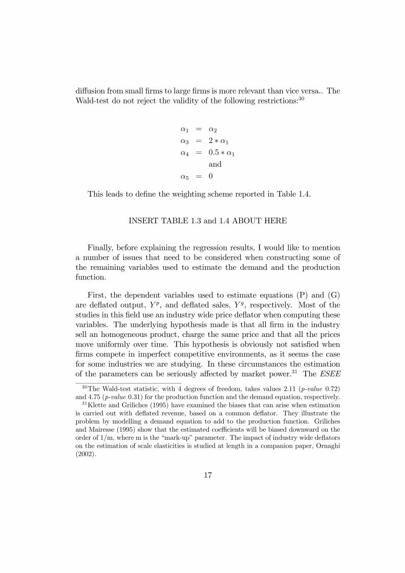
diffusion from small firms to large firms is more relevant than vice versa.. TheWald-test do not reject the validity of the following restrictions:30

α1 = α2

α3 = 2 ∗ α1α4 = 0.5 ∗ α1

and

α5 = 0

This leads to define the weighting scheme reported in Table 1.4.

INSERT TABLE 1.3 and 1.4 ABOUT HERE

Finally, before explaining the regression results, I would like to mentiona number of issues that need to be considered when constructing some ofthe remaining variables used to estimate the demand and the productionfunction.

First, the dependent variables used to estimate equations (P) and (G)are deflated output, Y p, and deflated sales, Y g, respectively. Most of thestudies in this field use an industry wide price deflator when computing thesevariables. The underlying hypothesis made is that all firm in the industrysell an homogeneous product, charge the same price and that all the pricesmove uniformly over time. This hypothesis is obviously not satisfied whenfirms compete in imperfect competitive environments, as it seems the casefor some industries we are studying. In these circumstances the estimationof the parameters can be seriously affected by market power.31 The ESEE

30The Wald-test statistic, with 4 degrees of freedom, takes values 2.11 (p-value 0.72)and 4.75 (p-value 0.31) for the production function and the demand equation, respectively.31Klette and Griliches (1995) have examined the biases that can arise when estimation

is carried out with deflated revenue, based on a common deflator. They illustrate theproblem by modelling a demand equation to add to the production function. Grilichesand Mairesse (1995) show that the estimated coefficients will be biased downward on theorder of 1/m, where m is the “mark-up” parameter. The impact of industry wide deflatorson the estimation of scale elasticities is studied at length in a companion paper, Ornaghi(2002).

17

reports the percentage change in the selling price applied by the firms. Thisallows us to express the output produced in terms of a reference year t. Byusing the log-difference transformation, we then get over the possible biasedintroduced by the existence of market power.32

Second, a proper measure of labour and physical capital has to take intoconsideration the intensity of utilisation of these variables. By using totalhours of work as labour input, L, and the rate of capacity utilisation, U , wehave a more satisfactory specification of the inputs of the production functionand consequently better estimates of the parameters can be obtained. As ex-plained in Appendix A, total number of hours is computed using the (mean)normal hours for each worker, plus overtime minus lost hours. This can pos-sibly lead to a measurement error due to rounding-off. I then use numberof employees (E) as instruments of the hours of work when estimating theproduction function.

Last, physical capital used in R&D laboratories and R&D employmenthave to be excluded from labour and capital measures since these inputsdo not produce current output. The database provides information on thenumber of employees engaged in R&D activities. This number is subtractedfrom the total employment reported by the firm when constructing the labourinput, L, and the relative instrument E. In this way I hope to minimisethe so called “double-counting” problem. On this point, Hall and Mairesse(1995) affirm that the most important correction is one related to the labourvariable.

4 Regression Results

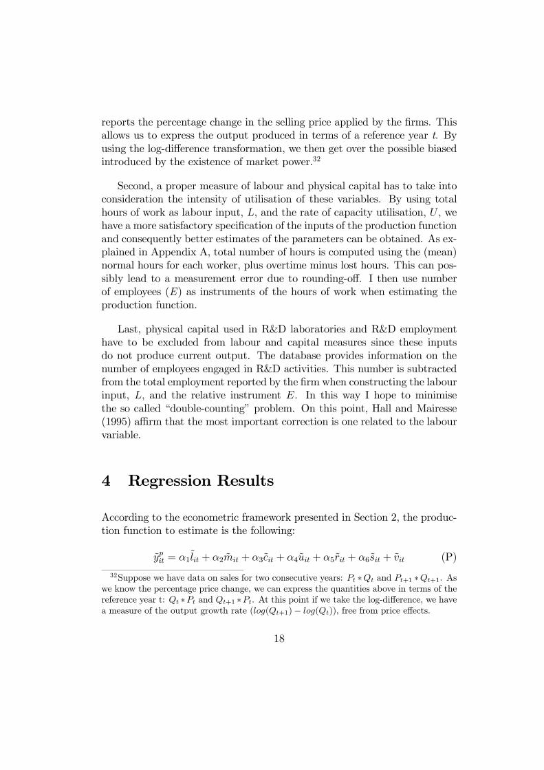
According to the econometric framework presented in Section 2, the produc-tion function to estimate is the following:

ypit = α1lit + α2mit + α3cit + α4uit + α5rit + α6sit + vit (P)

32Suppose we have data on sales for two consecutive years: Pt ∗Qt and Pt+1 ∗Qt+1. Aswe know the percentage price change, we can express the quantities above in terms of thereference year t: Qt ∗Pt and Qt+1 ∗Pt. At this point if we take the log-difference, we havea measure of the output growth rate (log(Qt+1)− log(Qt)), free from price effects.

18

Recall that small letters with tilde stand for log differences of the variablesnormalized with respect to the reference firm.

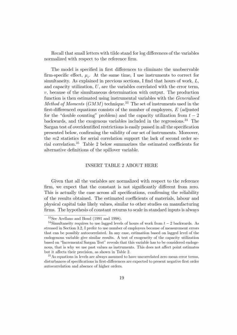
The model is specified in first differences to eliminate the unobservablefirm-specific effect, µi. At the same time, I use instruments to correct forsimultaneity. As explained in previous sections, I find that hours of work, L,and capacity utilization, U , are the variables correlated with the error term,v, because of the simultaneous determination with output. The productionfunction is then estimated using instrumental variables with the GeneralisedMethod of Moments (GMM) technique.33 The set of instruments used in thefirst-differenced equations consists of the number of employees, E (adjustedfor the “double counting” problem) and the capacity utilization from t − 2backwards, and the exogenous variables included in the regressions.34 TheSargan test of overidentified restrictions is easily passed in all the specificationpresented below, confirming the validity of our set of instruments. Moreover,the m2 statistics for serial correlation support the lack of second order se-rial correlation.35 Table 2 below summarizes the estimated coefficients foralternative definitions of the spillover variable.

INSERT TABLE 2 ABOUT HERE

Given that all the variables are normalized with respect to the referencefirm, we expect that the constant is not significantly different from zero.This is actually the case across all specifications, confirming the reliabilityof the results obtained. The estimated coefficients of materials, labour andphysical capital take likely values, similar to other studies on manufacturingfirms. The hypothesis of constant returns to scale in standard inputs is always

33See Arellano and Bond (1991 and 1998).34Simultaneity requires to use lagged levels of hours of work from t− 2 backwards. As

stressed in Section 3.2, I prefer to use number of employees because of measurement errorsthat can be possibly autocorrelated. In any case, estimation based on lagged level of theendogenous variable give similar results. A test of exogeneity of the capacity utilizationbased on “Incremental Sargan Test” reveals that this variable has to be considered endoge-nous, that is why we use past values as instruments. This does not affect point estimatesbut it affects their precision, as shown in Table 2.35As equations in levels are always assumed to have uncorrelated zero mean error terms,

disturbances of specifications in first-differences are expected to present negative first orderautocorrelation and absence of higher orders.

19

rejected at conventional significance level. This confirms a well known findingof most of the empirical studies on the production function: attempts tocontrol for unobservable heterogeneity and simultaneity gives unreasonablylow estimates of returns to scale.36 The coefficient of capacity utilizationshows a positive value but it is not precisely estimated, probably because itslagged levels turn out to be poor instruments.37

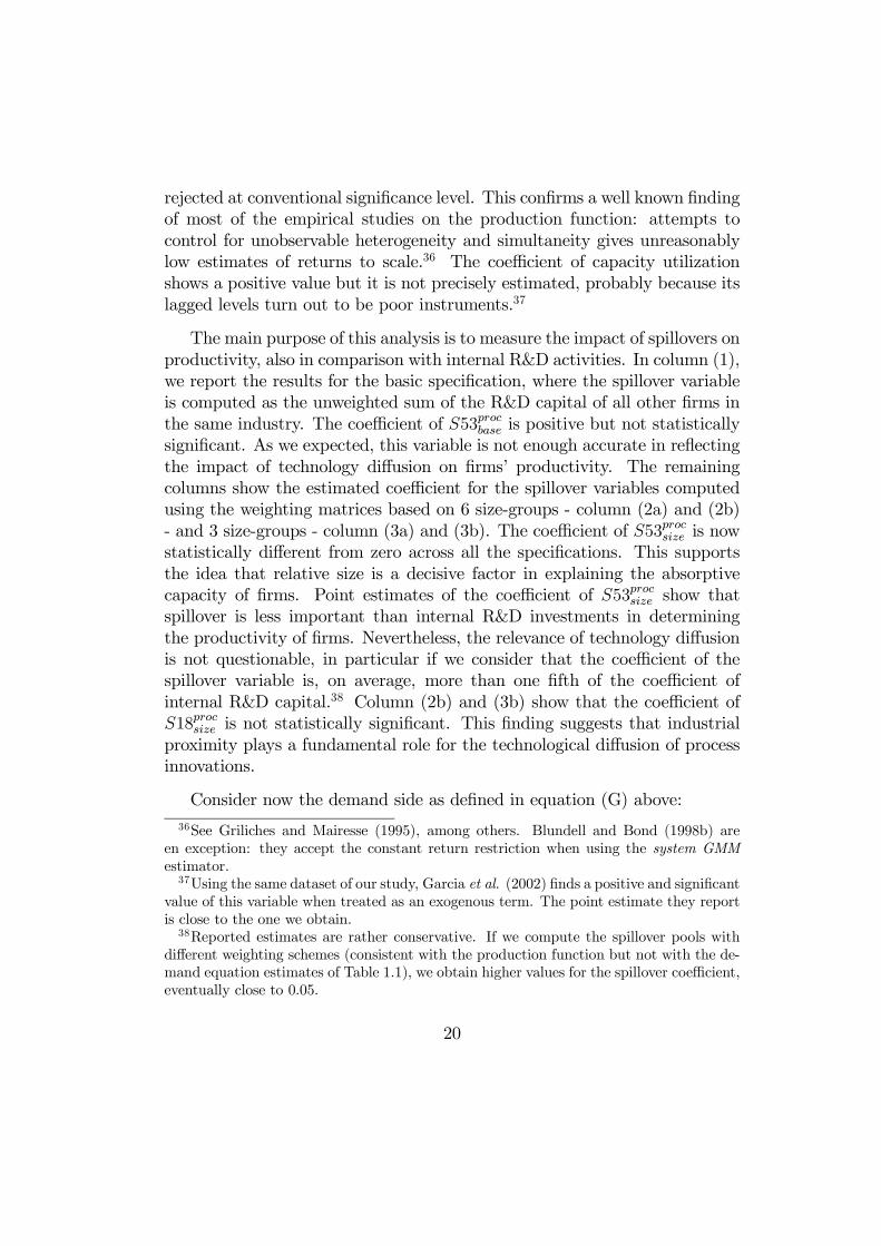
The main purpose of this analysis is to measure the impact of spillovers onproductivity, also in comparison with internal R&D activities. In column (1),we report the results for the basic specification, where the spillover variableis computed as the unweighted sum of the R&D capital of all other firms inthe same industry. The coefficient of S53procbase is positive but not statisticallysignificant. As we expected, this variable is not enough accurate in reflectingthe impact of technology diffusion on firms’ productivity. The remainingcolumns show the estimated coefficient for the spillover variables computedusing the weighting matrices based on 6 size-groups - column (2a) and (2b)- and 3 size-groups - column (3a) and (3b). The coefficient of S53procsize is nowstatistically different from zero across all the specifications. This supportsthe idea that relative size is a decisive factor in explaining the absorptivecapacity of firms. Point estimates of the coefficient of S53procsize show thatspillover is less important than internal R&D investments in determiningthe productivity of firms. Nevertheless, the relevance of technology diffusionis not questionable, in particular if we consider that the coefficient of thespillover variable is, on average, more than one fifth of the coefficient ofinternal R&D capital.38 Column (2b) and (3b) show that the coefficient ofS18procsize is not statistically significant. This finding suggests that industrialproximity plays a fundamental role for the technological diffusion of processinnovations.

Consider now the demand side as defined in equation (G) above:36See Griliches and Mairesse (1995), among others. Blundell and Bond (1998b) are

en exception: they accept the constant return restriction when using the system GMMestimator.37Using the same dataset of our study, Garcia et al. (2002) finds a positive and significant

value of this variable when treated as an exogenous term. The point estimate they reportis close to the one we obtain.38Reported estimates are rather conservative. If we compute the spillover pools with

different weighting schemes (consistent with the production function but not with the de-mand equation estimates of Table 1.1), we obtain higher values for the spillover coefficient,eventually close to 0.05.

20

ygit = β1epit + β2fadit + β3erit + β4esit + vit (G)

As explained in Section 2, the major econometric issue related to the de-mand relationship is the endogeneity of the price. Consequently, this variablehas been instrumented using lags from t− 2 to t − 5. The Sargan test con-firms the validity of the instruments used. Moreover, we fail to reject the nullhypothesis of absence of second order autocorrelation across all the specifi-cation reported in Table 3. The first three columns of this table presents theresults for the basic specification of the spillover variable while the remainingare based on the weighting scheme discussed above.

INSERT TABLE 3 ABOUT HERE

The constant always shows a small and not significant trend in the growthof real sales. The estimates for the price demand elasticity and advertisingshow the correct sign and are consistent with previous studies.39 As far asthe spillover effects are concerned, column (1a) shows a large negative co-efficient for the variable S53goodsize . Sales of firm i are negatively affected byany product improvements of competitors (competition effect). Neverthe-less, firm i can possibly take advantage of any innovation if it can learnand reproduce its contents (knowledge spillovers). It is not a simple task todisentangle these two opposite effects of competitors’ R&D investments onfirm i sales. The large and highly significant negative coefficient of S53goodsize

states that any firm whose variation of knowledge capital is inferior to therepresentative firm suffers a remarkable contraction in market shares. Thisvariable is then picking up the negative effect of competing against innov-ative firms.40 In order to isolate the (possible) positive effect of knowledgediffusion, it is necessary to augment the specification of the demand equa-tion with variables that control for the drop in sales due to the competitioneffect. A high relative growth rate of rivals’ R&D capital affects the evo-lution of the firm market share relative to its competitors once prices are

39See for instance Garcia et all. (2002).40Recall that the spillover variable is computed as the sum of rivals’ R&D capital; for

any two firms, this variable takes a higher value for the firm with lower R&D stock. SeeAppendix C for a simple numeric example.

21

controlled for. Hence, we can use the change of competitors’ market share(mrk share) as a proxy for the competition effect. Moreover, we can useindustry concentration (concen) as an overall measure of the impact of R&Dinvestments on market structure.41 Column (1c) in Table 3 shows that underthis new specification the coefficient of our spillover variable is now positive,although it is not statistically significant. Interestingly enough, the spillovervariable is the only one that records such a remarkable change: all the othervariables are rather stable across this alternative formulation. This suggeststhat these two new regressors are counting for the competition effect, with-out introducing any (relevant) mispecification of the demand equation. Thelow precision in estimating the technology diffusion effect call again for afiner definition of the spillover pools a firm can benefit from. Columns (2a)and (2b) and columns (3a) and (3b) show that the estimated coefficients forS53goodsize and S18

goodsize are positive and highly significant. This suggests that

learning from rivals plays a fundamental role when it comes to improving thequality of a product. Spanish firms are less R&D intensive than the averageof European firms. Therefore, it is possible that inward FDI works as chan-nels for knowledge spillovers.42 The coefficient of S18size and S53size are ofthe same order of magnitude, suggesting that technology diffusion goes wellbeyond a single sector when this is narrowly defined. As suggested in Sec-tion 2 spillover effects are potentially wide if we define an industry broadlyenough to consider vertical relations and complementary products. The re-sults presented give strong support to this intuitive reasoning. As before,we augment our demand equation with the variables mrk share and concenin order to drain the negative impact of rivals’ product innovation on firm isales due to competition. Results in column (3c) shows that the coefficientsof the spillover variables are practically identical to those reported in theother columns. This confirms that the computation of the spillover poolsusing relative size as a proxy for absorptive capacity is a reliable approachto disclose the existence and the magnitude of technological diffusion.

It is important to notice that the magnitude of spillovers for product andprocess innovations is rather different, also when compared to the internalR&D activities. Knowledge diffusion associated with product innovations is

41I am indebted to Bronwyn Hall for suggesting me this procedure.42Bertschek (1995) shows that imports and FDI play an important role for product and

process innovations in the case of German manufacturing firms. We are not aware of anyreliable study of this type for Spanish manufacturing industries.

22

larger in magnitude and extent. This implies that the standard approachbased on estimating the production function can only reveal part of the in-formation about spillovers while there are interesting and pervasive aspectof R&D externalities that cannot be quantify. This finding is related tothe point made by Quah (2002) in a study on the New Economy develop-ments. Although his focus is on economic growth and restricted to a particu-lar group of industries, his paper emphasises endogenous growth results fromthe interaction of demand and supply characteristics, not just production-side developments. In particular the author stresses (pag. 21) that “mostprofound changes in the New Economy are not productivity or supply-sideimprovements but instead consumption or demand side changes”.

5 Concluding Remarks

This paper analyses the impact of knowledge diffusion for product and processR&D. Our econometric frameworks modifies the standard approach first sug-gested by Griliches (1979) by adding a demand equation to the standard pro-duction function. To the best of my knowledge, there are no similar studiesin the empirical literature on spillovers. In constructing the components ofthe knowledge capital, I introduce two new features. First, as it is not in-novation input (R&D) but innovation output that has a positive impact onthe economic performance of a firm, I have modified the (standard) perpet-ual inventory method by introducing the notion of operative R&D capital.Second, the spillover variable is computed assuming that the chance of firmi borrowing knowledge from firm j depends on the relative size of the twofirms.

Our results suggest that knowledge spillovers play an important role inimproving the quality of products and, to a lesser extent, in increasing theproductivity of the firm. We find that technological diffusion of productinnovations is larger than the one of process innovations both in magnitudeand pervasiveness.

These findings have an interesting policy implication. If innovators areunable to appropriate the full benefits of their innovations, then the amount

23

of R&D may be lower than socially optimal, since firms consider only “pri-vate” returns on investments when planning their R&D activities. Fromour estimations, it emerges that the average gap between private and socialrates of return is higher for product innovation than for process innovation.This suggests the opportunity of a different public policy towards taxation ofR&D investments or government subsidies to R&D activities depending onthe type of innovation that firms are focused on. More evidence is obviouslyrequired before moving in this direction.

This analysis leaves some important questions unanswered. I have shownthat the magnitude of spillovers for product and process innovation is dif-ferent but further work is needed to determine the channels that actuallypermit knowledge to flow and how these differ between product and processinnovation. Process innovations are often linked to the skills of managers,engineers and technicians and competing firms can hardly benefit from theseinnovations. One possible channel is through mobility of R&D engineers.However, firms that are afraid of losing their technological advantages be-cause of this mobility can engage in simple, although costly, activities (e.g.,increasing wages and fringe benefits) designed at preventing their own em-ployees from leaving the firm. Product improvements are possibly simplerto learn and replicate, for example through reverse engineering. This line ofreasoning can explain the relevant discrepancy between diffusion of productand process innovations presented above. A recent attempt to determine themodels or mechanism that actually permit knowledge to flow is the work ofJaffe, Trajtenberg and Fogarty. (2000) based on case-studies of Americanfirms.

24

Appendix A: Data and VariableA1 Construction of Data SampleThe survey provides data on manufacturing firms with 10 or more em-

ployees. When this was designed, all firms with more than 200 employeeswere required to participate while a representative sample of about 5% of thefirms with 200 or less employees was randomly selected. In 1990, the firstyear of the panel, 715 firms with more than 200 employees were surveyed,which accounts for 68% of all the Spanish firms of this size. Newly estab-lished firms have been added every subsequent year to replace the exits dueto death and attrition.We start with a sample of 3,151 firms in an unbalanced panel data. The

total number of observations is 18,680. We then clean our dataset accordingto the following criteria:1) We remove all the observations with negative value added. There are

157 such observations, amounting to less than 1% of the original sample.2) We drop all observations where the quantity produced by the firm

doubled (or the growth rate is less than minus 50%) but there is not anincrease either in the number of employees or in the physical capital of atleast 50% (or a decrease of labour and capital less than minus 25%). Thisremoves 193 observations (about 1% of the initial sample).3) We remove all observations where the internal R&D capital records a

growth rate higher than 400%. This removes other 74 observations.In total, 424 observations are removed applying the filters above. The

subsample we use in our study consists of all the firms that have been sur-veyed for at least three years. There are 2,430 firms satisfying this condition,for a total number of 16,637 observations. At this point, we remove any ob-servations for which the data required to the estimation are not available. Inthe tables showing the results of the estimation, we report the exact numberof observations making up the final samples.

A2 Description of VariablesAdvertising (AD): Nominal amount of advertising expenditures deflated

by the firms’ output price.Capacity Utilization (U): Yearly average rate of capacity utilization re-

ported by the firmsCompetitors’ Market Share (Mrk share): We first determine firm i market

share (where the market is defined by the 3-digit CNAE code). Then, wedetermine the rivals’ share as 1 minus firm i market share.

25

Concentration (Concen): Herfindal index of industry concentration com-puted using the market share (as defined above) of all firms in the same3-digit industry.Employment (E): Approximation to the average number of works during

the year; it does not consider employees engaged in R&D activities.Labour (L): Labour consists of the total hours of work. It has been

constructed using the number of works, adjusted for the double counting ofR&D employees, times the normal hours plus overtime and minus lost hours.Materials (M): Nominal materials are given by the sum of purchases and

external services minus the variation of intermediate inventories. We usefirms’ specific deflator based on the variation in the cost of raw materialsand energy as reported by the firm.Operative R&D stocks for Process Innovations (Rproc): This variable is

constructed using the perpetual inventory method, assuming a depreciationrate of zero (ρ = 0). The word “operative” specifies that only successfulinnovation is considered in our empirical estimation. Computation is fullyexplained in Section 3.2.Operative R&D stocks for Product Innovations (Rgood): As for the vari-

able Rproc above, R&D expenditures are capitalized only when firms achievea product innovation. See Section 3.2 for further detail.Output (Y p): Nominal output is defined as the sum of sales and the

variation of inventories. We deflate the nominal amount using the firms’sspecific output price as defined belowPhysical Capital (C): It has been constructed capitalising firms’ invest-

ments in machinery and equipment and using sectorial rates of depreciation.The capital stock does not include buildings. This variable is taken fromMartin and Suarez (1997).Price (P): Paasche type price index calculated from the variation of price

reported in the ESEE. This variable is not expressed in levels but in growthrate. It is used to estimate the price elasticities in the demand equation andto deflate nominal output.Sales (Y g): Amount of total sales reported by the firms deflated by firms’

specific output price as defined below.Size Weighted Spillovers (S53 size): Sum of R&D capital of other firms

in the same industry as defined by the 53-sector classification, weighted bythe size of the firms. We use two different weighting matrices as explainedin Section 3.2Size Weighted Spillovers (S18 size): Sum of others’ R&D capital in the

26

same industry as defined by the 18-sector classification, weighted by the sizeof the firms, minus the R&D stocks of the firms in the same industry at53-sector classification. We use two different weighting matrices as explainedin Section 3.2Unweighted Spillovers (S53 basic): Unweighted sum of the R&D capital of

other firms in the same industry at 53-sector classification.Unweighted Spillovers (S18 basic): Unweighted sum of others’ R&D capital

in the same industry at 18-sector classification, minus the R&D stocks of thefirms in the same industry at 53-sector classification.

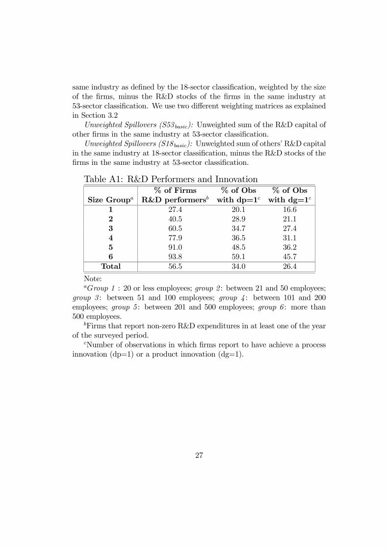
Table A1: R&D Performers and Innovation% of Firms % of Obs % of Obs

Size Groupa R&D performersb with dp=1c with dg=1c

1 27.4 20.1 16.62 40.5 28.9 21.13 60.5 34.7 27.44 77.9 36.5 31.15 91.0 48.5 36.26 93.8 59.1 45.7

Total 56.5 34.0 26.4

Note:aGroup 1 : 20 or less employees; group 2 : between 21 and 50 employees;

group 3 : between 51 and 100 employees; group 4 : between 101 and 200employees; group 5 : between 201 and 500 employees; group 6 : more than500 employees.

bFirms that report non-zero R&D expenditures in at least one of the yearof the surveyed period.

cNumber of observations in which firms report to have achieve a processinnovation (dp=1) or a product innovation (dg=1).

27

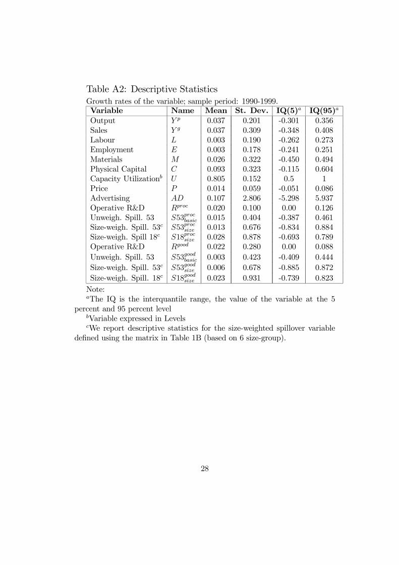
Table A2: Descriptive StatisticsGrowth rates of the variable; sample period: 1990-1999.Variable Name Mean St. Dev. IQ(5)a IQ(95)a

Output Y p 0.037 0.201 -0.301 0.356Sales Y g 0.037 0.309 -0.348 0.408Labour L 0.003 0.190 -0.262 0.273Employment E 0.003 0.178 -0.241 0.251Materials M 0.026 0.322 -0.450 0.494Physical Capital C 0.093 0.323 -0.115 0.604Capacity Utilizationb U 0.805 0.152 0.5 1Price P 0.014 0.059 -0.051 0.086Advertising AD 0.107 2.806 -5.298 5.937Operative R&D Rproc 0.020 0.100 0.00 0.126Unweigh. Spill. 53 S53procbasic 0.015 0.404 -0.387 0.461Size-weigh. Spill. 53c S53procsize 0.013 0.676 -0.834 0.884Size-weigh. Spill 18c S18procsize 0.028 0.878 -0.693 0.789Operative R&D Rgood 0.022 0.280 0.00 0.088Unweigh. Spill. 53 S53goodbasic 0.003 0.423 -0.409 0.444Size-weigh. Spill. 53c S53goodsize 0.006 0.678 -0.885 0.872Size-weigh. Spill. 18c S18goodsize 0.023 0.931 -0.739 0.823Note:aThe IQ is the interquantile range, the value of the variable at the 5

percent and 95 percent levelbVariable expressed in LevelscWe report descriptive statistics for the size-weighted spillover variable

defined using the matrix in Table 1B (based on 6 size-group).

28

Appendix B: Errors in VariableAs discussed in Section 3.2, we put a lot of efforts in determining firms’

internal R&D stocks. We consider all possible source of investments (intra-mural, contracted outside and imported technology), we test for alternativeinitial values and we take into consideration the (supposed) timing whenR&D investments are expected to affect the productivity and the demandfaced by the firm (the “operative” capital). Although we are aware that ourvariable R cannot be considered a perfect measure of the internal R&D capi-tal, we feel confident that it is not affected by (relevant) measurement errors.Point estimates reported in Section 4 are close to other studies and seem toconfirm our view. A possible alternative generally employed in the contextof panel data is to use past values of the endogenous variable as instruments.Unfortunately, the R&D capital is highly persistent and lags of this variablein levels turn out to be poor instruments to estimate equations in differences.We also tried to use R&D employees as an external instruments. However,the Sargan test rejects the validity of this approach.Note that the bias due to measurement errors is negative when the coef-

ficients for the internal R&D stock is positive (see Arellano (2000)). There-fore, if we find a positive and significant relationship between productivityand demand changes and internal R&D capital, we might argue that the truerelationship is even stronger.

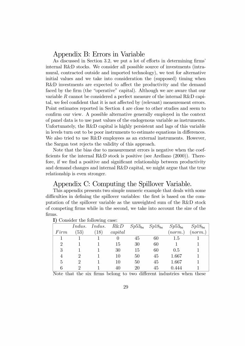
Appendix C: Computing the Spillover Variable.This appendix presents two simple numeric example that deals with some

difficulties in defining the spillover variables: the first is based on the com-putation of the spillover variable as the unweighted sum of the R&D stockof competing firms while in the second, we take into account the size of thefirms.I) Consider the following case:

Indus. Indus. R&D Sp53ba Sp18ba Sp53ba Sp18baFirm (53) (18) capital (norm.) (norm.)1 1 1 0 45 60 1.5 12 1 1 15 30 60 1 13 1 1 30 15 60 0.5 14 2 1 10 50 45 1.667 15 2 1 10 50 45 1.667 16 2 1 40 20 45 0.444 1

Note that the six firms belong to two different industries when these

29

are defined by the 53-industry classification but they all belong to the sameindustry when we use the broader 18 sector classification. For any firm i,the variable SP53basic (column 5) is defined as the sum of the R&D stock(column 4) of all the other firms in the same industry (for the 53-industryclassification). SP18basic (column 6) is computed as the sum of the R&Dstock of all the other firms in the same industry at 18-sector classificationexcluding SP53basic. Recall that we normalize all the variables w.r.t. their 3-digit CNAE industry averages, before proceeding to the empirical estimation(to keep things simple, we suppose that the CNAE classification correspondsto the 53-industry classification in column 2). The last two columns reportthe values of the spillover variables after this normalization. We can drawtwo main insights from this example: i) a higher value of SP53basic necessaryindicates a lower internal R&D capital; ii) it is not possible to use SP18basicin a regression since it takes value 1 for all the firms.II) Consider, now, this second example, where we compute the spillover

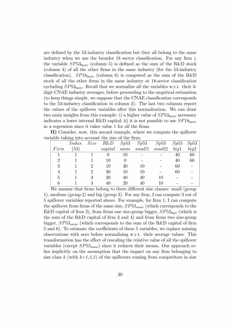
variable taking into account the size of the firm:Indus. Size R&D Sp53 Sp53 Sp53 Sp53 Sp53

Firm (53) capital same small1 small2 big1 big21 1 1 0 10 - - 40 602 1 1 10 0 - - 40 603 1 2 10 30 10 - 60 -4 1 2 30 10 10 - 60 -5 1 3 20 40 40 10 - -6 1 3 40 20 40 10 - -

We assume that firms belong to three different size classes: small (group1), medium (group 2) and big (group 3). For any firm, I can compute 3 out of5 spillover variables reported above. For example, for firm 1, I can computethe spillover from firms of the same size, SP53same (which corresponds to theR&D capital of firm 2), from firms one size-group bigger, SP53big1 (which isthe sum of the R&D capital of firm 3 and 4) and from firms two size-groupbigger, SP53same (which corresponds to the sum of the R&D capital of firm5 and 6). To estimate the coefficients of these 5 variables, we replace missingobservations with zero before normalizing w.r.t. their average values. Thistransformation has the effect of rescaling the relative value of all the spillovervariables (except SP53same) since it reduces their means. Our approach re-lies implicitly on the assumption that the impact on any firm belonging tosize class k (with k=1,2,3 ) of the spillovers coming from competitors in size

30

class k+s (with | s |≤ 2) depends on s but not on k (e.g. SP53small1 mea-sures technology diffusion from median firm to big firm and from small firmto medium firm, at the same time). Although this modus operandi can beopen to criticism, we need to observe that: i) the sources and channels oftechnology diffusion are so complex that any approach used to get a proxyfor the spillover pools can be criticized and defended at the same time. Wefeel that the differences in size (more than the absolute size of the firm) canplay an important role in defining differences in the absorptive capacity; ii)we check for the robustness of our results (in particular to the replacementof missing observations with zeros) by defining two different size classifica-tion (one with 6 groups and the other with 3 groups) and we obtain similarand sensible results, as discussed in Section 3.2; moreover, estimations havebeen run also using the balanced panel sample with no sensible differences inthe results obtained (so that these are robust also to changes in the samplecomposition); iii) the estimated coefficients of these variables are not used tomake inferences about spillover in product and process innovation (the ulti-mate objective of our analysis) but are simply used as weights to compute afiner spillover variable than the basic one. We could impose similar weightsex-ante (on the base of some assumptions) without going through this pro-cedure. For example, we compute the spillover variable summing only theR&D stocks of all the firms of the same size or smaller (this is equivalent toa weighting matrix with value 1 if size(firm i)≥size(firm j ) and zero other-wise). We find that the general results presented in Section 4 are still validunder this (ad hoc) approach.

31

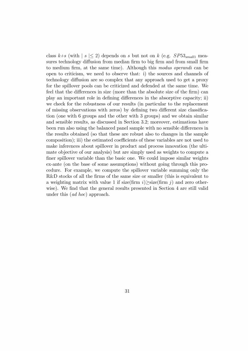
Appendix D: Definition of Industrial SectorsThe ESEE reports the 3-digit CNAE sector that firms belong to. There

are 122 different manufacturing sectors. To construct the spillover variables,we defined two different industrial classification: one grouping those 3-digitsectors into 53 industries and another one into 18 industries. In other words,the sectors defined by the CNAE has been grouped into 53 industries andthe later has been successively grouped into 18 (larger) industries.

Table D1: 18 Industry ClassificationSector Definition 3-digit CNAE1 Ferrous and non ferrous metals 221 to 2242 Non-metallic minerals 240 to 2493 Chemical products 251 to 2554 Metal products 311 to 3195 Industrial and agricultur machinery 321 to 3296 Office and data processing machine 330, 391 to 3997 Electrical and electronic goods 341 to 347, 351

to 3558 Vehicles, cars and motors 361 to 3639 Other transport equipment 371 to 372, 381

to 38910 Meat and preserved meat 41311 Food and tobacco 411 to 412, 414

to 423, 42912 Beverages 424 to 42813 Textiles and clothing 431 to 439, 453

to 45614 Leather and shoes 441 to 442, 451

to 45215 Timber and furniture 461 to 46816 Paper and printing products 471 to 47517 Rubber and Plastic products 481 to 48218 Other manufacturing products 491 to 495

32

Table D2: 53 Industry ClassificationSector Definition 3-digit CNAE1 Ferrous and non ferrous metals 221 to 2242 Structural clay products 240 to 2413 Concrete 242, 248 to 2494 Concrete mixer and other by-products 2435 Stone and ceramic 244 to 245, 2476 Glass 2467 Inorganic and organic chemicals and syn-

tetic materials251 to 252

8 Paints, Varnishes and other chemicalproducts

253

9 Drugs 25410 Soap and Detergents 25511 Metal foundaries and primary smelting

and refining311 to 313

12 Fabricated structural metal products(doors, frames, ..)

314

13 Heating equipment 315, 31914 Miscellaneous metal products (bolts, nuts,

screws, ..)316

15 Farm machinery and equipment 32116 Metal work machinery and textile

machinery322 to 323

17 Machinery for chemical industry 32418 Mining and construction machinery and

convey equipments325 to 326

19 Engines and turbines and other machiner-ies, not elsewhere classified

327 to 329

20 Office equipments and medical and photo-graphic instruments

330, 391 to 399

21 Electric transmission and wiringequipment

341 to 342

22 Electrical industrial apparatus 343 to 34423 Houshold appliances 34524 Electric lightening 346

33

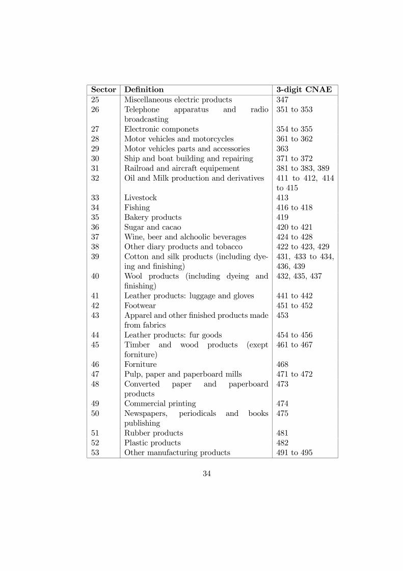
Sector Definition 3-digit CNAE25 Miscellaneous electric products 34726 Telephone apparatus and radio

broadcasting351 to 353

27 Electronic componets 354 to 35528 Motor vehicles and motorcycles 361 to 36229 Motor vehicles parts and accessories 36330 Ship and boat building and repairing 371 to 37231 Railroad and aircraft equipement 381 to 383, 38932 Oil and Milk production and derivatives 411 to 412, 414

to 41533 Livestock 41334 Fishing 416 to 41835 Bakery products 41936 Sugar and cacao 420 to 42137 Wine, beer and alchoolic beverages 424 to 42838 Other diary products and tobacco 422 to 423, 42939 Cotton and silk products (including dye-

ing and finishing)431, 433 to 434,436, 439

40 Wool products (including dyeing andfinishing)

432, 435, 437

41 Leather products: luggage and gloves 441 to 44242 Footwear 451 to 45243 Apparel and other finished products made

from fabrics453

44 Leather products: fur goods 454 to 45645 Timber and wood products (exept

forniture)461 to 467

46 Forniture 46847 Pulp, paper and paperboard mills 471 to 47248 Converted paper and paperboard

products473

49 Commercial printing 47450 Newspapers, periodicals and books

publishing475

51 Rubber products 48152 Plastic products 48253 Other manufacturing products 491 to 495

34

References[1] Arellano, M. (2000), “Panel Data Econometrics”, Chap. 4, still unpub-

blised.

[2] Arellano, M. and Bond S. (1998), “Dynamic Panel Data Estimationusing DPD98 for Gauss: A Guide for Users”, Oxford University.

[3] Arellano, M. and Bond S. (1991), “Some Test of Specification for PanelData: Monte Carlo Evidence and an Application to Employment Equa-tions”. Review of Economic Studies, Vol. 58, pp. 277-297.

[4] Benito, P. (2000), “R&D Productivity and Spillovers: Evidence fromSpanish Panel Data”, Ph D. Thesis, Chap. 1, Universidad de Valencia.

[5] Bertschek, I. (1995), “Product and Process Innovation as a Responseto Increasing Imports and Foreign Direct Investment”. The Journal ofIndustrial Economics, Vol.43, pp. 341-357.

[6] Blundell, R.W. and Bond S.R. (1998a), “Initial Conditions and MomentRestrictions in Dynamic Panel Data Models”. Journal of Econometrics,Vol. 87, pp. 115-143.

[7] Blundell, R.W. and Bond S.R. (2000), “GMM estimation with PersistentPanel Data: An Application to Production Functions”. EconometricReviews, Vol. 19, pp. 321-340.

[8] Cassiman, B. and Veugelers R.(1999) “R&D Cooperation and Spillovers:Some Empirical Evidence”, CEPR Discussion Paper, No. 2330.

[9] Garcia, A., Jaumandreu, J. and Rodriguez C. (2002), “Innovation andJobs: Evidence from Manufacturing Firms”. mimeo, Universidad CarlosIII de Madrid.

[10] Greene, W. H. (1997), “Econometric Analysis”. Prentice-Hall Interna-tional, London.

[11] Griliches, Z (1992), “The Search for R&D Spillovers”. ScandinavianJournal of Economics, Vol. 94, pp. S29-47.

[12] Griliches, Z. (1979), “Issues in Assessing the Contribution of R&D toProductivity Growth”. Bell Journal of Economics, Vol. 10, pp. 92-116.

35

[13] Griliches, Z. and Mairesse J. (1995), “Production Function: The Searchfor Indentification”. NBER Working Paper, No. 5067.

[14] Griliches, Z. andMairesse J. (1984), “Productivity and R&D at the FirmLevel”. In R&D, Patents and Productivity, ed. Zvi Griliches. Universityof Chicago Press.

[15] Hall, B.H and Mairesse J. (1995), “Exploring the Relationship betweenR&D and Productivity in French Manufacturing Firms”. Journal ofEconometrics, Vol. 65, pp. 263-293.

[16] Hall, B.H. Griliches Z. and Hausman J.A. (1986), “Is there a second(technological opportunity) factor?”. International Economic Review,Vol. 27, pp. 265-283.

[17] Hernan, R., Marin, P. and Siotis G. (2003) “An Empirical Evaluationof the Determinants of Research Joint Venture Formation”, Journal ofIndustrial Economics, forthcoming.

[18] Hulten, C.R. (2000), “Total Factor Productivity: A short Biography”.NBER Working Paper, No. 7471.

[19] Instituto Nacional de Estadistica (1999), Estadistica sobre actividadesen investigación cientificas y desarollo tecnológico, Spain.

[20] Jaffe, A.B. (1986), “Technological Opportunity and Spillovers of R&D:Evidence from Firms’ Patents, Profits, and Market Value”. AmericanEconomic Review, Vol. 76, pp. 984-1001.

[21] Jaffe. A.B. Trajtenberg M. and Fogarty M.S. (2000), “KnowledgeSpillovers and Patent Citations: Evidence from a Survey of Inventors”,American Economic Review, Vol. 90, pp. 215-218.

[22] Klette, T.J. (1999), “Market Power, Scale Economies and Productiv-ity: Estimates from a Panel of Establishment Data”. The Journal ofIndustrial Economics, Vol. 48, pp. 451-476.

[23] Klette, T.J. (1996), “R&D, Scope Economies, and Plant Performance”.RAND Journal of Economics, Vol. 27, pp. 502-522.

36

[24] Klette, T.J. and Griliches Z (1996), “The inconsistency of CommonScale Estimators when Output Prices are Unobserved and Endogenous”.Journal of Applied Econometrics, Vol. 11, pp. 343-361.

[25] Levin, R.C. and Reiss P.C. (1988), “Cost-reducing and Demand-creatingR&Dwith Spillovers”. RAND Journal of Economics, Vol. 19, pp538-556.

[26] Los, B. and Verspagen B. (2000), “R&D Spillovers and Productivity:Evidence from U.S. Manufacturing Microdata”. Empirical Economics,Vol. 25, pp. 127-148.

[27] Mansfield, E. (1983), “Technological Change and Market Structure: AnEmpirical Study”. American Economic Review, Vol. 73, pp. 205-209.

[28] Mansfield, E., Rapoport J., Romeo A., Wagner S., and Beardsley G.(1977), “Social and Private Rates of Return from Industrial Innovation-s”. Quarterly Journal of Economics, Vol. 41, pp. 221-240.

[29] Marin, P., Siotis G. and Hernan R. (2000) “An Empirical Evaluationof the Determinants of Research Joint Venture Formation”, CEPR Dis-cussion Paper, No. 2442.

[30] Martin, A. and Suarez C. (1997), “El Stock de Capital para las Em-presas de la Encuesta sobre Estrategias Empresariales”. Documento In-terno n.13, Programa de Investigaciones Económicas, Fundación Em-presa Pública.

[31] Nadiri, M.I. (1993), “Innovation and Technological Spillovers”. NBERWorking Paper, No. 4423.

[32] Ornaghi, C. (2002), “Assessing the Effects of Measurement Errors on theEstimation of the Production Function”. mimeo, Universidad Carlos IIIde Madrid.

[33] Pakes, A. and Schankerman M. (1984), “The Rate of Obsolescence ofPatents, Research Gestation Lags, and the Private Rate of Return to Re-search Resources”. In R&D, Patents and Productivity, ed. Zvi Griliches.University of Chicago Press.

[34] Quah, D. (2002), “Technology Dissemination and Economic Growth:Some Lessons for the New Economy”. CEPR Discussion Paper, No.3207.

37

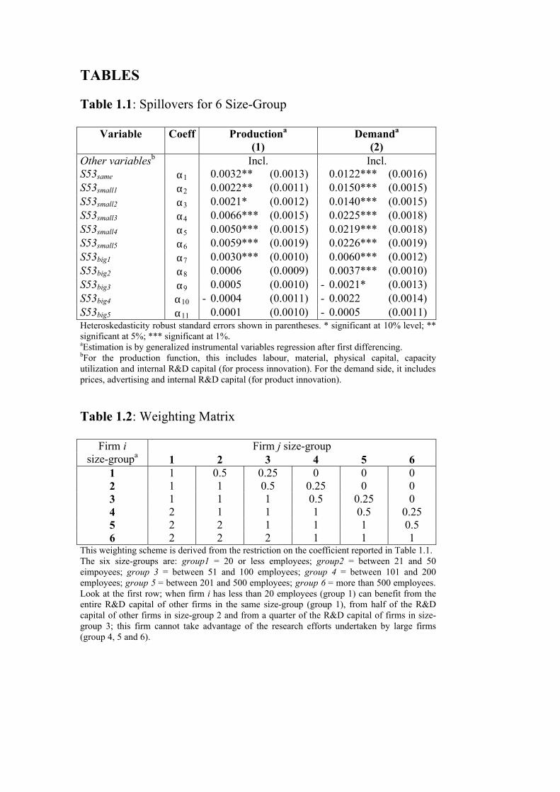
TABLES Table 1.1: Spillovers for 6 Size-Group

Variable Coeff Productiona

(1) Demanda

(2) Other variablesb Incl. Incl. S53same α1 0.0032** (0.0013) 0.0122*** (0.0016) S53small1 α2 0.0022** (0.0011) 0.0150*** (0.0015) S53small2 α3 0.0021* (0.0012) 0.0140*** (0.0015) S53small3 α4 0.0066*** (0.0015) 0.0225*** (0.0018) S53small4 α5 0.0050*** (0.0015) 0.0219*** (0.0018) S53small5 α6 0.0059*** (0.0019) 0.0226*** (0.0019) S53big1 α7 0.0030*** (0.0010) 0.0060*** (0.0012) S53big2 α8 0.0006 (0.0009) 0.0037*** (0.0010) S53big3 α9 0.0005 (0.0010) - 0.0021* (0.0013) S53big4 α10 - 0.0004 (0.0011) - 0.0022 (0.0014) S53big5 α11 0.0001 (0.0010) - 0.0005 (0.0011) Heteroskedasticity robust standard errors shown in parentheses. * significant at 10% level; ** significant at 5%; *** significant at 1%. aEstimation is by generalized instrumental variables regression after first differencing. bFor the production function, this includes labour, material, physical capital, capacity utilization and internal R&D capital (for process innovation). For the demand side, it includes prices, advertising and internal R&D capital (for product innovation). Table 1.2: Weighting Matrix

Firm j size-group Firm i size-groupa 1 2 3 4 5 6

1 1 0.5 0.25 0 0 0 2 1 1 0.5 0.25 0 0 3 1 1 1 0.5 0.25 0 4 2 1 1 1 0.5 0.25 5 2 2 1 1 1 0.5 6 2 2 2 1 1 1

This weighting scheme is derived from the restriction on the coefficient reported in Table 1.1. The six size-groups are: group1 = 20 or less employees; group2 = between 21 and 50 eimpoyees; group 3 = between 51 and 100 employees; group 4 = between 101 and 200 employees; group 5 = between 201 and 500 employees; group 6 = more than 500 employees. Look at the first row; when firm i has less than 20 employees (group 1) can benefit from the entire R&D capital of other firms in the same size-group (group 1), from half of the R&D capital of other firms in size-group 2 and from a quarter of the R&D capital of firms in size-group 3; this firm cannot take advantage of the research efforts undertaken by large firms (group 4, 5 and 6).

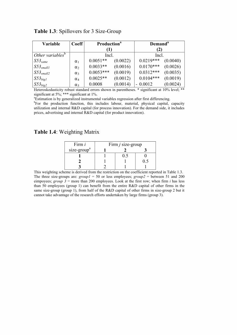
Table 1.3: Spillovers for 3 Size-Group

Variable Coeff Productiona

(1) Demanda

(2) Other variablesb Incl. Incl. S53same α1 0.0051** (0.0022) 0.0219*** (0.0040) S53small1 α2 0.0033** (0.0016) 0.0170*** (0.0026) S53small2 α3 0.0053*** (0.0019) 0.0312*** (0.0035) S53big1 α4 0.0025** (0.0012) 0.0104*** (0.0019) S53big2 α5 0.0008 (0.0014) - 0.0012 (0.0024) Heteroskedasticity robust standard errors shown in parentheses. * significant at 10% level; ** significant at 5%; *** significant at 1%. aEstimation is by generalized instrumental variables regression after first differencing. bFor the production function, this includes labour, material, physical capital, capacity utilization and internal R&D capital (for process innovation). For the demand side, it includes prices, advertising and internal R&D capital (for product innovation).

Table 1.4: Weighting Matrix

Firm j size-group Firm i size-groupa 1 2 3

1 1 0.5 0 2 1 1 0.5 3 2 1 1

This weighting scheme is derived from the restriction on the coefficient reported in Table 1.3. The three size-groups are: group1 = 50 or less employees; group2 = between 51 and 200 eimpoyees; group 3 = more than 200 employees. Look at the first row; when firm i has less than 50 employees (group 1) can benefit from the entire R&D capital of other firms in the same size-group (group 1), from half of the R&D capital of other firms in size-group 2 but it cannot take advantage of the research efforts undertaken by large firms (group 3).

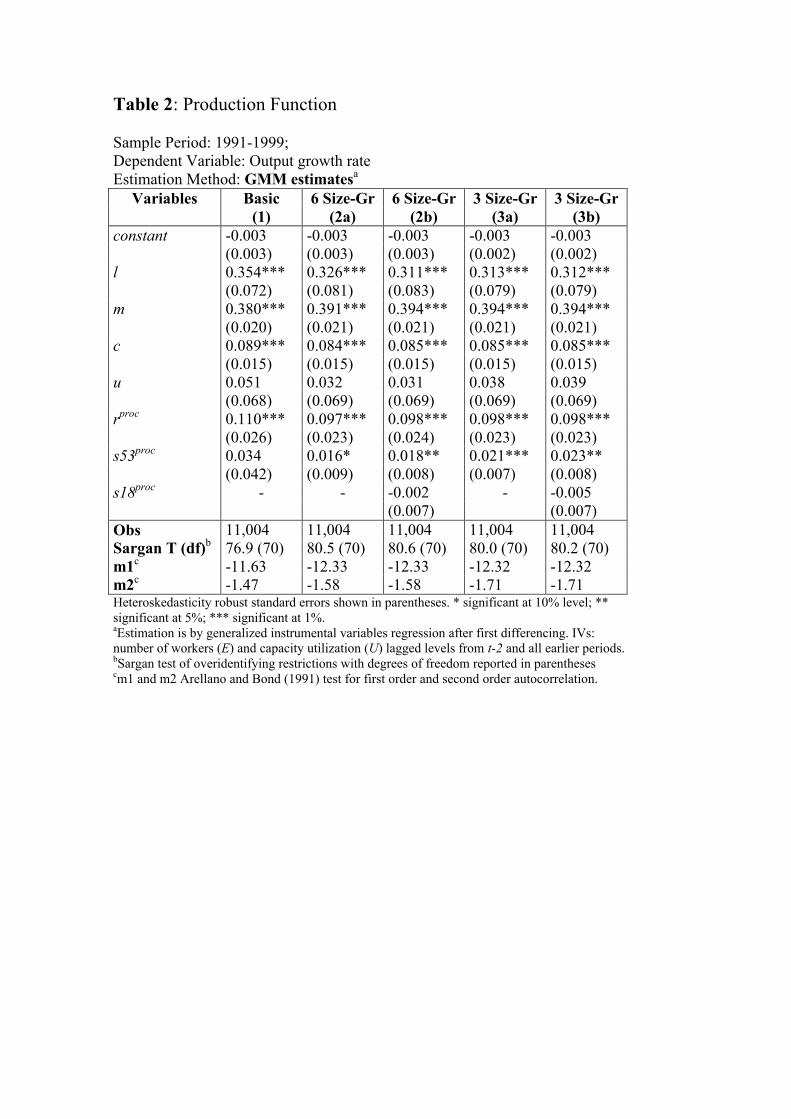
Table 2: Production Function Sample Period: 1991-1999; Dependent Variable: Output growth rate Estimation Method: GMM estimatesa

Variables Basic 6 Size-Gr 6 Size-Gr 3 Size-Gr 3 Size-Gr (1) (2a) (2b) (3a) (3b)

constant -0.003 -0.003 -0.003 -0.003 -0.003 (0.003) (0.003) (0.003) (0.002) (0.002) l 0.354*** 0.326*** 0.311*** 0.313*** 0.312*** (0.072) (0.081) (0.083) (0.079) (0.079) m 0.380*** 0.391*** 0.394*** 0.394*** 0.394*** (0.020) (0.021) (0.021) (0.021) (0.021) c 0.089*** 0.084*** 0.085*** 0.085*** 0.085*** (0.015) (0.015) (0.015) (0.015) (0.015) u 0.051 0.032 0.031 0.038 0.039 (0.068) (0.069) (0.069) (0.069) (0.069) rproc 0.110*** 0.097*** 0.098*** 0.098*** 0.098*** (0.026) (0.023) (0.024) (0.023) (0.023) s53proc 0.034 0.016* 0.018** 0.021*** 0.023** (0.042) (0.009) (0.008) (0.007) (0.008) s18proc - - -0.002 - -0.005 (0.007) (0.007) Obs 11,004 11,004 11,004 11,004 11,004 Sargan T (df)b 76.9 (70) 80.5 (70) 80.6 (70) 80.0 (70) 80.2 (70) m1c -11.63 -12.33 -12.33 -12.32 -12.32 m2c -1.47 -1.58 -1.58 -1.71 -1.71 Heteroskedasticity robust standard errors shown in parentheses. * significant at 10% level; ** significant at 5%; *** significant at 1%. aEstimation is by generalized instrumental variables regression after first differencing. IVs: number of workers (E) and capacity utilization (U) lagged levels from t-2 and all earlier periods. bSargan test of overidentifying restrictions with degrees of freedom reported in parentheses cm1 and m2 Arellano and Bond (1991) test for first order and second order autocorrelation.

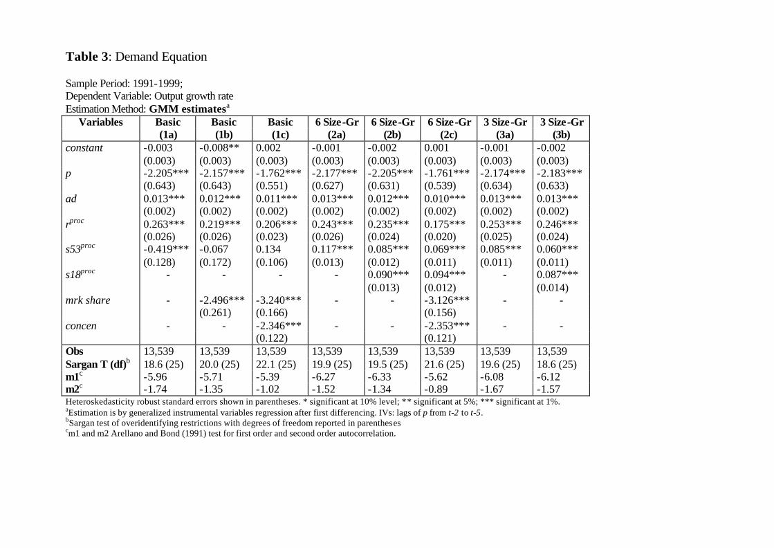
Table 3: Demand Equation Sample Period: 1991-1999; Dependent Variable: Output growth rate Estimation Method: GMM estimatesa

Variables Basic Basic Basic 6 Size-Gr 6 Size-Gr 6 Size-Gr 3 Size-Gr 3 Size-Gr (1a) (1b) (1c) (2a) (2b) (2c) (3a) (3b)

constant -0.003 -0.008** 0.002 -0.001 -0.002 0.001 -0.001 -0.002 (0.003) (0.003) (0.003) (0.003) (0.003) (0.003) (0.003) (0.003) p -2.205*** -2.157*** -1.762*** -2.177*** -2.205*** -1.761*** -2.174*** -2.183*** (0.643) (0.643) (0.551) (0.627) (0.631) (0.539) (0.634) (0.633) ad 0.013*** 0.012*** 0.011*** 0.013*** 0.012*** 0.010*** 0.013*** 0.013*** (0.002) (0.002) (0.002) (0.002) (0.002) (0.002) (0.002) (0.002) rproc 0.263*** 0.219*** 0.206*** 0.243*** 0.235*** 0.175*** 0.253*** 0.246*** (0.026) (0.026) (0.023) (0.026) (0.024) (0.020) (0.025) (0.024) s53proc -0.419*** -0.067 0.134 0.117*** 0.085*** 0.069*** 0.085*** 0.060*** (0.128) (0.172) (0.106) (0.013) (0.012) (0.011) (0.011) (0.011) s18proc - - - - 0.090*** 0.094*** - 0.087*** (0.013) (0.012) (0.014) mrk share - -2.496*** -3.240*** - - -3.126*** - - (0.261) (0.166) (0.156) concen - - -2.346*** - - -2.353*** - - (0.122) (0.121) Obs 13,539 13,539 13,539 13,539 13,539 13,539 13,539 13,539 Sargan T (df)b 18.6 (25) 20.0 (25) 22.1 (25) 19.9 (25) 19.5 (25) 21.6 (25) 19.6 (25) 18.6 (25) m1c -5.96 -5.71 -5.39 -6.27 -6.33 -5.62 -6.08 -6.12 m2c -1.74 -1.35 -1.02 -1.52 -1.34 -0.89 -1.67 -1.57 Heteroskedasticity robust standard errors shown in parentheses. * significant at 10% level; ** significant at 5%; *** significant at 1%. aEstimation is by generalized instrumental variables regression after first differencing. IVs: lags of p from t-2 to t-5. bSargan test of overidentifying restrictions with degrees of freedom reported in parentheses cm1 and m2 Arellano and Bond (1991) test for first order and second order autocorrelation.