WIDER Working Paper 2018/6

Fiscal multipliers in South Africa

The importance of financial sector dynamics

Konstantin Makrelov,1 Channing Arndt,2 Rob Davies,3 and Laurence Harris4

January 2018

1 National Treasury, Pretoria, South Africa, and School of Financial and Management Studies, SOAS University of London, London, UK, corresponding author: konstantinmakrelov@gmail.com; 2 International Food Policy Research Institute (IFPRI), Washington, DC, USA, and School of Financial and Management Studies, SOAS University of London, London, UK; 3 School of Financial and Management Studies, SOAS University of London, London, UK; 4 School of Financial and Management Studies, SOAS University of London, London, UK.

This study has been prepared within the UNU-WIDER project ‘Southern Africa—Towards inclusive economic development (SA-TIED)’.

Copyright © UNU-WIDER 2018

Information and requests: publications@wider.unu.edu

ISSN 1798-7237 ISBN 978-92-9256-448-3

Typescript prepared by Luke Finley.

The United Nations University World Institute for Development Economics Research provides economic analysis and policy advice with the aim of promoting sustainable and equitable development. The Institute began operations in 1985 in Helsinki, Finland, as the first research and training centre of the United Nations University. Today it is a unique blend of think tank, research institute, and UN agency—providing a range of services from policy advice to governments as well as freely available original research.

The Institute is funded through income from an endowment fund with additional contributions to its work programme from Denmark, Finland, Sweden, and the United Kingdom.

Katajanokanlaituri 6 B, 00160 Helsinki, Finland

The views expressed in this paper are those of the author(s), and do not necessarily reflect the views of the Institute or the United Nations University, nor the programme/project donors.

Abstract: We analyse implications of financial sector dynamics for fiscal expenditure multipliers in recessionary conditions. We employ a stock-and-flow-consistent model for South Africa with four financial instruments and detailed balance sheets for the household, government, financial, non-financial, and foreign sectors, and the Reserve Bank. The increase in government expenditure positively affects the probability of default, valuations, and perceptions of risk. Higher inflows of foreign savings can increase the multiplier further by reducing the domestic savings constraint. The size of the fiscal multipliers is also dependent on the actions of domestic and foreign monetary authorities, thus emphasizing the importance of policy co-ordination.

Keywords: stock-and-flow consistent, financial dynamics, fiscal multipliers, South Africa JEL classification: C68, D53, D58, E44, E62

Acknowledgements: We are grateful for comments from Christopher Adam and Bassam Fattouh and support from the United Nations University World Institute for Development Economics Research.

1

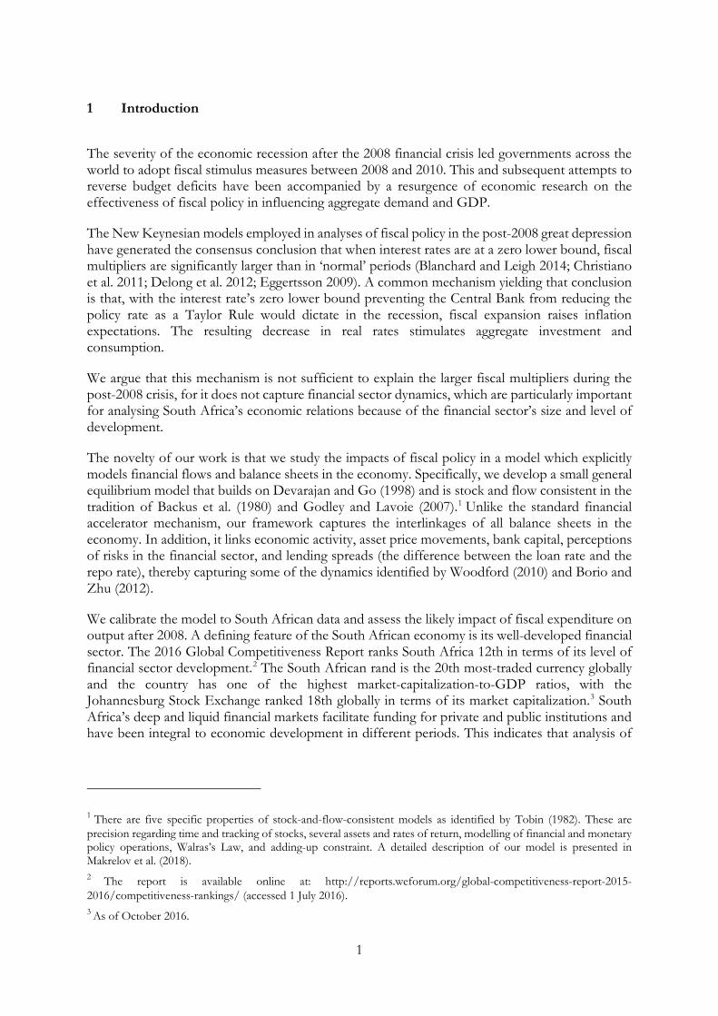
1 Introduction

The severity of the economic recession after the 2008 financial crisis led governments across the world to adopt fiscal stimulus measures between 2008 and 2010. This and subsequent attempts to reverse budget deficits have been accompanied by a resurgence of economic research on the effectiveness of fiscal policy in influencing aggregate demand and GDP.

The New Keynesian models employed in analyses of fiscal policy in the post-2008 great depression have generated the consensus conclusion that when interest rates are at a zero lower bound, fiscal multipliers are significantly larger than in ‘normal’ periods (Blanchard and Leigh 2014; Christiano et al. 2011; Delong et al. 2012; Eggertsson 2009). A common mechanism yielding that conclusion is that, with the interest rate’s zero lower bound preventing the Central Bank from reducing the policy rate as a Taylor Rule would dictate in the recession, fiscal expansion raises inflation expectations. The resulting decrease in real rates stimulates aggregate investment and consumption.

We argue that this mechanism is not sufficient to explain the larger fiscal multipliers during the post-2008 crisis, for it does not capture financial sector dynamics, which are particularly important for analysing South Africa’s economic relations because of the financial sector’s size and level of development.

The novelty of our work is that we study the impacts of fiscal policy in a model which explicitly models financial flows and balance sheets in the economy. Specifically, we develop a small general equilibrium model that builds on Devarajan and Go (1998) and is stock and flow consistent in the tradition of Backus et al. (1980) and Godley and Lavoie (2007).1 Unlike the standard financial accelerator mechanism, our framework captures the interlinkages of all balance sheets in the economy. In addition, it links economic activity, asset price movements, bank capital, perceptions of risks in the financial sector, and lending spreads (the difference between the loan rate and the repo rate), thereby capturing some of the dynamics identified by Woodford (2010) and Borio and Zhu (2012).

We calibrate the model to South African data and assess the likely impact of fiscal expenditure on output after 2008. A defining feature of the South African economy is its well-developed financial sector. The 2016 Global Competitiveness Report ranks South Africa 12th in terms of its level of financial sector development.2 The South African rand is the 20th most-traded currency globally and the country has one of the highest market-capitalization-to-GDP ratios, with the Johannesburg Stock Exchange ranked 18th globally in terms of its market capitalization.3 South Africa’s deep and liquid financial markets facilitate funding for private and public institutions and have been integral to economic development in different periods. This indicates that analysis of

1 There are five specific properties of stock-and-flow-consistent models as identified by Tobin (1982). These are precision regarding time and tracking of stocks, several assets and rates of return, modelling of financial and monetary policy operations, Walras’s Law, and adding-up constraint. A detailed description of our model is presented in Makrelov et al. (2018). 2 The report is available online at: http://reports.weforum.org/global-competitiveness-report-2015-2016/competitiveness-rankings/ (accessed 1 July 2016). 3 As of October 2016.

2

fiscal policy in the South African context needs to consider interactions through both the financial sector and the real economy.

Our results indicate that the expenditure fiscal multiplier in South Africa was in the range of 2 to 3 in the period immediately after the 2008 financial crisis, given the negative output gap, the low government-debt-to-GDP ratio, the monetary policy stance, the health of the South African financial sector, and the large inflow of foreign savings into the economy. Our results differ significantly from those of recent studies on South Africa and studies looking at the size of fiscal multipliers in other emerging markets. The absence of Ricardian households in our framework, the lack of supply-side constraints, the unresponsiveness of monetary authorities to the closing but still negative output gap (similar to zero-bound interest rate conditions), and, most importantly, the presence of stock-and-flow-consistent financial sector dynamics amplify the impact of a fiscal stimulus.

In the model, the causal chain runs as follows. Higher fiscal expenditure increases aggregate demand, stimulating domestic economic activity in the presence of idle resources. Factor incomes increase, improving firms’ profitability and household income. This translates into higher deposits with banks. The supply of loans increases as there are more deposits with the financial sector. Following the mechanisms outlined by Borio and Zhu (2012) and Woodford (2010), the acceleration in economic activity reduces the probability of default and the perception of risk, and improves valuations and the net worth of the financial sector, leading to higher levels of intermediation and lower lending spreads. The decline in lending spreads stimulates economic activity further, creating a feedback loop which operates through the balance sheets of all agents, unlike the financial accelerator mechanism proposed by Bernanke et al. (1999). The effect depends on the inflows of foreign savings, which reduce the savings constraint facing the domestic economy and allow investment expenditure to accelerate. This result is in line with the theoretical model of Blanchard et al. (2016). In the absence of foreign savings, the higher multiplier is primarily driven by the higher levels of household consumption, as higher equity prices make it easier for the representative household to achieve its target level of wealth.

Our result relies on low debt agents or credit unconstraint agents—in this case government— expanding demand and fuelling a financial accelerator mechanism. The latter depends on the health of the financial sector. In a stock-and-flow-consistent framework, this implies that the deterioration in the net worth of government is offset by an improvement in the net worth of other agents. In the South African context, the non-financial enterprise and foreign sectors have seen improvements in their net worth while the household and government sectors have recorded deteriorations in their net worth.

The rest of the paper proceeds as follows. In Section 2, we review the relevant literature. Section 3 provides an overview of the South African fiscal system and fiscal policy since the 2008 financial crisis. The model framework and the data are discussed in Sections 4 and 5, respectively. Section 6 presents the results and Section 7 concludes.

2 Literature review

The mainstream theoretical mechanism for assessing the size of fiscal multipliers relies on New Keynesian dynamics, which have been built into dynamic stochastic general equilibrium (DSGE) models (Christiano et al. 2005; Smets and Wouters 2007). The critical assumptions affecting the size of the fiscal multipliers are monetary policy driven by a Taylor Rule and inflation consistent with a New Keynesian Phillips curve, Ricardian households, and rational expectations combined

3

with limited or no financial frictions and sticky prices and wages. Under the Taylor Rule specification, an increase in aggregate demand will narrow the output gap, pushing the policy rate (even if the output gap is still negative) directly through the Taylor Rule and indirectly through its impact on inflation via the Phillips curve. Fiscal expansion causes a rise in real interest rates which, in turn, affects consumption and investment negatively and leads to the familiar crowding-out effect.

The Ricardian households anticipate that current fiscal expenditure will have to be offset by higher taxes in the future as they have perfect knowledge of government inter-temporal constraints. This leads households to increase savings to compensate for the impact of higher taxes in the future on their permanent income, leading to lower household consumption now. The absence of financial frictions assumes away any financial accelerator effects that may amplify the positive or negative effects associated with fiscal policy decisions. The effect is offset somewhat by the assumption of sticky prices and wages, which amplifies aggregate demand effects.

Coenen (2012) studies the impact of expansionary fiscal policy in seven structural DSGE models used heavily by policymaking institutions and compares the results with two academic DSGE models. In his study, monetary accommodation and a higher share of non-Ricardian households increase the multipliers significantly. Lower nominal rigidities translate into higher multipliers as they increase the inflationary impacts and decrease real rates in the presence of monetary accommodation. Coenen acknowledges that the absence of financial frictions can underestimate the size of the fiscal multipliers in DSGE models.

Recent empirical research indicates that fiscal multipliers tend to be larger during recessionary periods (Auerbach and Gorodnichenko 2012; Fazzari et al. 2015; Owyang et al. 2013; Riera-Crichton et al. 2015).4 Such asymmetry is inconsistent with the underlying theoretical mechanisms in the New Keynesian DSGE framework.

Following the 2008 financial crisis the models have been published with analyses of the expansionary potential of fiscal policy in a recession when the policy interest rate is at a zero lower bound, a situation that was effectively reached in the United States, the United Kingdom, and the Eurozone as the Federal Reserve, Bank of England, and European Central Bank lowered interest rates to near zero (Blanchard and Leigh 2014; Christiano et al. 2011; Delong et al. 2012; Eggertsson 2009). For example, Christiano et al. (2011) find a spending multiplier of 3.7 under zero lower bound conditions compared with a multiplier of 1.1 under normal conditions. Eggertsson (2009) finds a spending multiplier of 2.3 under zero lower bound conditions compared with 0.5 under normal conditions.

In the presence of a zero lower bound that prevents nominal interest rates falling to adjust real interest rates towards the level that would be required by a standard monetary policy rule, higher government expenditure pushes inflation expectations up, thereby reducing real rates and stimulating private consumption and investment. In a second-round effect, the reduced output gap leads to a further rise in inflation expectations and stimulates the economy (Christiano et al. 2011). Effectively, the Taylor Rule mechanism is switched off at zero nominal interest rates, causing real rates to fall as inflation expectations rise.

4 For example, Auerbach and Gorodnichenko (2012) find a spending multiplier of 2.4 in recessionary conditions, while Owyang et al. (2013) find a multiplier of 1.6 for Canada. Mineshima et al. (2014) provide a comprehensive review of the recent literature on fiscal multipliers for advanced countries, and Batini et al. (2014) for emerging economies.

4

The multiplier effect is likely to be stronger if the fiscal expansion is driven by measures supporting aggregate demand rather than aggregate supply, as the latter tends to increase the spare capacity in the economy and deflationary pressures (Coenen 2012; Eggertsson 2009).5

In addition, the assumption regarding Ricardian households is less binding, as the number of credit-constrained households increases in economic conditions characterized by zero lower bound. The Ricardian equivalence theorem relies on assumptions such as absence of credit constraints on households and similar interest rates and time horizons for government and households. There is no evidence that these assumptions hold, particularly during times of economic slowdown.6

Eggertsson and Krugman (2012) present a different theoretical model to explain the higher multipliers under zero lower bound conditions, which operates via the real stock of debt. In their framework, liquidity-constrained debtors are forced to repay debt, and thus their spending depends on current rather than expected future income. Under conditions characterized by zero bounds on nominal interest rates, expansionary fiscal policy can stop the deflationary spiral, reduce the stock of real debt, and halt the deleveraging process, which in turn eases the credit constraint and supports further expansion in output. Their model works through inflation, rather than expected inflation as in Christiano et al. (2011).

Some recent DSGE models assume that Ricardian equivalence does not hold for all households by introducing a certain share of credit-constrained households. In Gali et al. (2007), the size of the multiplier varies with the share of rule-of-thumb households and the degree of price stickiness. Higher price stickiness reduces the mark-up in the presence of a fiscal expansion. A similar mechanism is employed by Cogan et al. (2010). However, they find a lower multiplier, as their study uses a lower share of credit-constrained households and wage rigidities, which reduces the impact of fiscal expansion on household income.

A limitation of the New Keynesian framework and the related DSGE models is the absence of financial sector dynamics. This is particularly important since recessionary conditions are often a by-product of financial sector crises, which also cause more severe economic slowdowns, accompanied by weaker recoveries (Reinhart and Rogoff 2009). Financial markets are also the main determinant of the sustainability of government debt and thus the effectiveness of fiscal policy (Afonso et al. 2011; Mittnik and Semmler 2013).7 For example, Proaño et al. (2014) find that at high levels of financial stress the government-debt-to-GDP level has a negative impact on economic activity, regardless of the debt levels.8

Studies employing New Keynesian models have addressed the lack of financial sector dynamics by introducing the financial accelerator mechanism proposed by Bernanke et al. (1999). A fall in net worth implies that borrowers have little wealth to contribute to project finance. This creates a potential divergence between the interests of borrowers and those of lenders, which increases

5 The level of hysteresis can have a significant impact on the size of the fiscal multipliers, and thus even fiscal expansion measures which support aggregate supply may have a strong positive impact on output (Delong et al. 2012). 6 Carlin and Soskice (2015) provide discussion of the conditions required in order for the Ricardian equivalence theorem to hold. 7 The empirical literature generally finds that high government debt levels are associated with small or negative multipliers (Huidrom et al. 2016; Nickel and Tudyka 2014). 8 Studies that do not take into account financial sector dynamics find that the threshold level varies between 70 and 90 per cent on average, depending on the sample of countries studied, with developing countries likely to have lower threshold levels (Caner et al. 2010; Elmeskov and Sutherland 2012; Reinhart and Rogoff 2010).

5

agency costs in the presence of asymmetric information. The probability of default increases because the company has less of its own funds involved in the project. The higher agency costs require that the lenders are compensated through higher premiums, which increase the external finance constraints for firms. In a second-round effect, the higher premiums lead to a further reduction in net wealth and amplify the initial effect. This effect can start with a fall in economic activity, which reduces cash flows, asset prices, and profits, reducing net worth. Bernanke et al. (1999) illustrate the impact of a government expenditure shock in their model. The presence of the financial accelerator mechanism magnifies the impact of an increase in government expenditure, mainly through its impact on asset prices and the related increase in firms’ net worth.

A number of studies employ the financial accelerator model in a DSGE framework to study the impact of fiscal expansion on output. Fernández-Villaverde (2010) and Carrillo and Poilly (2010) find that the size of the fiscal multiplier increases significantly in the presence of financial frictions, which work through the balance sheet of a representative firm.9 Higher government expenditure increases inflation, which reduces the real value of the debt stock of firms. The mechanism is similar to that of Eggertsson and Krugman (2012). This improves net worth and, through the financial accelerator mechanism, magnifies the positive impact of the fiscal expansion.

Merola (2012) also employs the financial accelerator framework, which amplifies the transmission mechanism identified by Christiano et al. (2011). The combination of nominal interest rates at the zero lower bound and a financial accelerator mechanism increases the fiscal multipliers.10 The presence of financial frictions and zero lower bound conditions generates fiscal multipliers of similar size to those generated by Fernández-Villaverde (2010) and Carrillo and Poilly (2010) and significantly lower that the multipliers produced by Christiano et al. (2011) and Eggertsson (2009). Counterintuitively, it appears that the presence of financial frictions reduces the size of fiscal multipliers.

Kollmann et al. (2013) extend the financial accelerator model to the financial sector. In their framework the impact works through the link between the net worth of the representative bank and the spread between the mortgage rate and the deposit rate. A loan default lowers bank capital, increases the spread, and reduces output.11 This assumes that the financial accelerator mechanism applied to banks is similar to that applied to firms. The financial sector, however, has the important role of intermediation and money creation. A fall in the net worth of the financial sector has much broader implications than a fall in the net worth of other agents in the economy, by increasing lending spreads but also by reducing the supply of intermediation services and the money multiplier (Woodford 2010). The decline in intermediation services exacerbates credit constraints in the economy and leads to a further decline in asset prices and the net worth of banks. Continuous deterioration in the balance sheet of the financial sector leads eventually to insolvency and a banking crisis.

The challenge with the financial accelerator mechanism is that it appears that only the net worth of one sector’s balance sheet is important to economic activity. The balance sheets of different

9 While the presence of financial sector dynamics increases the size of the fiscal multiplier, these effects are small and the multipliers are significantly lower than those found by Christiano et al. (2011) and Eggertsson (2009). The multiplier moves from just below 1 to just above 1 in the presence of financial frictions and zero lower bound conditions. 10 If nominal interest rates are not at the zero bound, then the size of the multipliers decreases significantly as the real interest rate channel identified by Merola (2012) is no longer operational. 11 The financial accelerator mechanism embedded in the balance sheet of banks is also used to study unconventional monetary policy questions in DSGE models (Gertler and Karadi 2011; Gertler et al. 2012).

6

sectors of the economy and their interlinkages are not captured. These interlinkages can strengthen or weaken the transmission of shocks through the financial sector. In the absence of stock consistency, the mechanism cannot capture the distribution of debt, which is important to determine the sustainability of expansionary fiscal policy and the likely fiscal multiplier. More importantly, the financial accelerator mechanism is not able to capture the dynamics of risk-taking as it ignores the time-varying pricing of risk and effective risk tolerance (Borio and Zhu 2012).

The omission of the foreign sector in the financial accelerator mechanism implies that the impacts of increased global liquidity are not captured. In models without financial sector dynamics, higher inflows will translate into an appreciation in the currency and a contraction in domestic activity. However, in models with financial dynamics and a foreign sector, increased global liquidity and higher inflow of foreign savings can reduce the domestic savings constraint, increase credit extension and asset prices, and support a fiscal expansion.12 In the theoretical framework of Blanchard et al. (2016), higher inflows of foreign savings appreciate the currency but also reduce the cost of financial intermediation. If the latter effect dominates the former effect, the inflow of foreign capital can be expansionary. Their framework, however, does not capture financial accelerator mechanisms and thus it may underestimate the impacts.

Since current New Keynesian models of fiscal policy omit other sectors’ balance sheets, compositional issues are ignored and there is no consistent representation of flow-of-funds information between institutions. This generates results which can be misleading. For example, Fernández-Villaverde (2010) and Carrillo and Poilly (2010) argue that a cut in labour taxes will reduce inflation in the economy by increasing the supply of labour, and will hence reduce the fiscal multipliers. But lower labour taxes can increase the cash flow of households, improve their balance sheets, and reduce their credit constraints, which can increase the size of the multipliers. This channel is missing in their analysis. There is general equilibrium on the real side of the economy but only partial dynamics on the financial side.

These are significant limitations to the current New Keynesian framework and the associated DSGE models, as the presence of financial sector dynamics, which satisfy stock and flow consistency, can have a significant impact on the size of the fiscal multipliers. That this is so is indicated by empirical findings of a strong relationship between risk premiums and asset prices on the one side and the impact of fiscal policy on the other (Afonso et al. 2011; Afonso and Sousa 2012; Agnello and Sousa 2013; Proaño et al. 2014).

Fiscal decisions can affect the balance sheets and net worth of all institutions in the economy. The financial sector will affect the real economy through the borrower balance sheet channel, the bank balance sheet channel, and the liquidity channel, as identified by BCBS (2011). The financial accelerator effect will work through not only the net worth of non-financial firms but also the net worth of all institutions in the economy and the complex inter-relationships that exist between the assets and liabilities of different institutions. The impacts will also work through the theoretical model of Borio and Zhu (2012) and Woodford (2010).

In the model developed by Woodford (2010), the lending spread is a function of the financial sector capital. Raising the level of capital is costly and leverage is limited by regulatory requirements. Shocks that impair the capital of the intermediary or higher leverage ratio regulatory requirements translate into higher lending spreads and lower volumes of lending and economic activity. Borio and Zhu (2012) also link the capital of the financial sector to bank behaviour. In

12 The importance of global liquidity and capital flows relates the current discussion to the literature on monetary policy independence and the global financial cycle. For more information see Rey (2015).

7

their framework, the behaviour is driven by the capital threshold effect and the capital framework effect. The capital threshold effect arises because breaching the minimum threshold is costly for a bank. In the face of a possible breach, banks will take defensive action to avoid the high costs, which will affect the availability and pricing of funding extended to customers. The capital framework effect influences the way the banks measure, manage, and price risk, which affects their behaviour. The economic cycle changes the strength of the capital threshold effect as probability of default, valuations, and the perception of risk change. In turn, this shifts the relative position of the banks’ capital to the regulatory threshold and affects bank behaviour. The accelerator effects in both models are driven by the relationship between capital and economic activity. Higher economic activity reduces the probability of default and the perception of risk, and improves valuations. This reduces lending spreads, which encourages further improvements in economic activity.

The implication of these mechanisms for fiscal policy is that expansionary fiscal policy which is perceived as sustainable may have a much stronger impact on the economy than the current estimates in the economic literature, through its impact on economic activity directly and indirectly via its impact on bank capital. At the same time, unsustainable expansion could have a much more negative impact than currently anticipated.

In addition, balance sheet dynamics play an important role in understanding how funding of government expenditure affects the economy. For example, the financial sector facilitates the movement of funds from non-government institutions to government. If funders disinvest from other asset classes, this will affect the price of these assets and possibly the net worth of some individuals and companies.13 This will have broader implications for the economy. The financial sector’s alternative of raising funds from households to purchase government bonds will depend on the health of balance sheets in the economy. Similarly, fiscal decisions to fund expenditure through direct taxes can affect after-tax income and profits, and the ability of households to service their debt and of companies to provide dividends. This can also have implications for institutional balance sheets and the net worth of market participants. If no other institutions are willing to purchase government bonds due to the health of their balance sheets, it will be left to the Central Bank to purchase them, reducing the fiscal expansion to unconventional monetary policy (Borio and Disyatat 2010). Capturing these relationships requires a model closure of stock and flow consistency.

Recent studies on fiscal multipliers in South Africa do not incorporate financial sector dynamics. Jooste et al. (2013), employing a DSGE model, a structural vector error correction model, and a time-varying parameter vector autoregressive model, find that countercyclical fiscal policy has been effective in South Africa; however, the impact has often been less than unity in the short term and there is no impact on GDP in the long term. The largest multiplier is reached after five quarters and is equivalent to 0.6. These authors argue that the small multiplier reflects high imports leakage, which is common for open economies. Mabugu et al. (2013), employing an inter-temporal CGE model, find that government expenditure can have a positive impact if it is on investment, and this translates into higher productivity. Other types of expenditure tend to have very small multipliers.14 Akanbi (2013) uses a macroeconometric model to study the impacts of fiscal policy in South Africa and finds that multipliers associated with demand-side interventions tend to be smaller if the

13 In addition to issues of net worth, if for example equity prices fall, market values will fall and investment can decline through a Tobin’s Q process. 14 The model seems to be supplied constraint, and only interventions which increase the supply side of the economy lead to positive multipliers with a significant lag.

8

economy is supply-side constrained. Generally, the multipliers are just below 1 even in conditions characterized by a negative output gap, and decline to zero within three years of the shock.

Our framework is also different to those of studies of other emerging market economies. These also have no financial dynamics and the multipliers tend to be small. Such studies do not identify specific periods or conditions which affect the size of the multipliers. The results are based on time-series analysis, dominated by vector autoregressive techniques, which average the impact of fiscal decisions on the economies over a fairly long period of time in order to satisfy requirements regarding the number of observations. Thus, they provide limited insights into whether, under recessionary conditions with falling asset prices, fiscal multipliers are large or small, and what drives their magnitude.

Jha et al. (2014) employ a structural vector autoregressive (SVAR) model to study the impacts of tax cuts and government expenditure in ten Asian economies. They find that, on average, tax cuts have a greater countercyclical impact on output than government expenditure. They argue that tax cuts stimulate investment, unlike higher government consumption expenditure, which crowds out investment. They show the present values of cumulative spending multipliers, which vary from negative 3.3 in Thailand after nine quarters to positive 1.3 in India. The tax multipliers vary between negative 1.5 in Thailand and positive 2.2 in India. This result is somewhat contradicted by Hur et al. (2014). They find, employing both a panel data model and a SVAR model for the same ten Asian economies, that there is no significant relationship between fiscal expenditure and consumption and investment.

Jawadi et al. (2014) employ a similar methodology along with a smooth transition regression model to study fiscal policy in Brazil, Russia, India, and China. Their results indicate that government spending tends to have a stronger impact than a reduction in taxes in all countries except India. A decline in taxes led to an increase in output in Brazil and China and a contraction in Russia, and had no impact in India.

Our structural model allows us to capture the specific conditions around the 2008 crisis, the strong fiscal response, and some unique features of the South African economy, such as a very well-developed financial sector and high tax compliance. This is in contrast to emerging markets, which are generally characterized by large informal sectors and fairly low levels of financial development (Batini et al. 2014).

3 South Africa’s fiscal environment

South Africa’s fiscal system is based on three spheres of government: national, provincial, and local. The Constitution provides guidelines for the types of expenditure for which each sphere of government is responsible. For example, national government is responsible for expenditure having a national dimension, such as defence, tertiary education, and foreign affairs. Provincial and national governments share responsibilities in areas such as primary and secondary education and health, while local government is responsible for expenditure on areas of municipal significance such as water and electricity reticulation, cemeteries, and local sports facilities. The division of revenue is entrenched in law and is guided by the Division of Revenue Bill, which distributes resources across the different spheres of government. Tax policy falls under the domain of national government. Provincial governments have limited revenue-generating power and are only allowed to borrow under very limited circumstances, while local governments have some significant revenue-generating instruments such as property rates and service charges, and they can also

9

borrow.15 While the political system is quasi-federal, the fiscal system is more centralized, with the revenue powers lying largely with the national government. The national government also has important oversight responsibilities for all spheres of government, including state-owned companies, through the Public Finance Management Act and Municipal Finance Management Act. The institutional framework ensues that national government, and particularly the National Treasury, is responsible for fiscal policy.

South Africa’s fiscal position was strong at the beginning of the financial crisis. Gross and net debt levels were between 20 and 30 per cent. As economic activity contracted in 2009, the output gap widened. Klein (2011) reports an output gap of negative 2.4 per cent and negative 1.4 per cent for 2009 and 2010, respectively. Ehlers et al. (2013) calculate similar-sized output gaps, while estimating slightly more negative output gaps. These estimates take into account the scaling up of fiscal expenditure over the period. The combination of low government debt, under-utilization of economic resources, and a well-functioning financial sector16 created the conditions for a countercyclical increase in government expenditure. Real government consumption expenditure increased by 5.8 and 4.6 per cent in 2008 and 2009, well above the average economy-wide growth rate. Consumption expenditure remained close to or just above average growth in economic activity in 2010 and 2011.

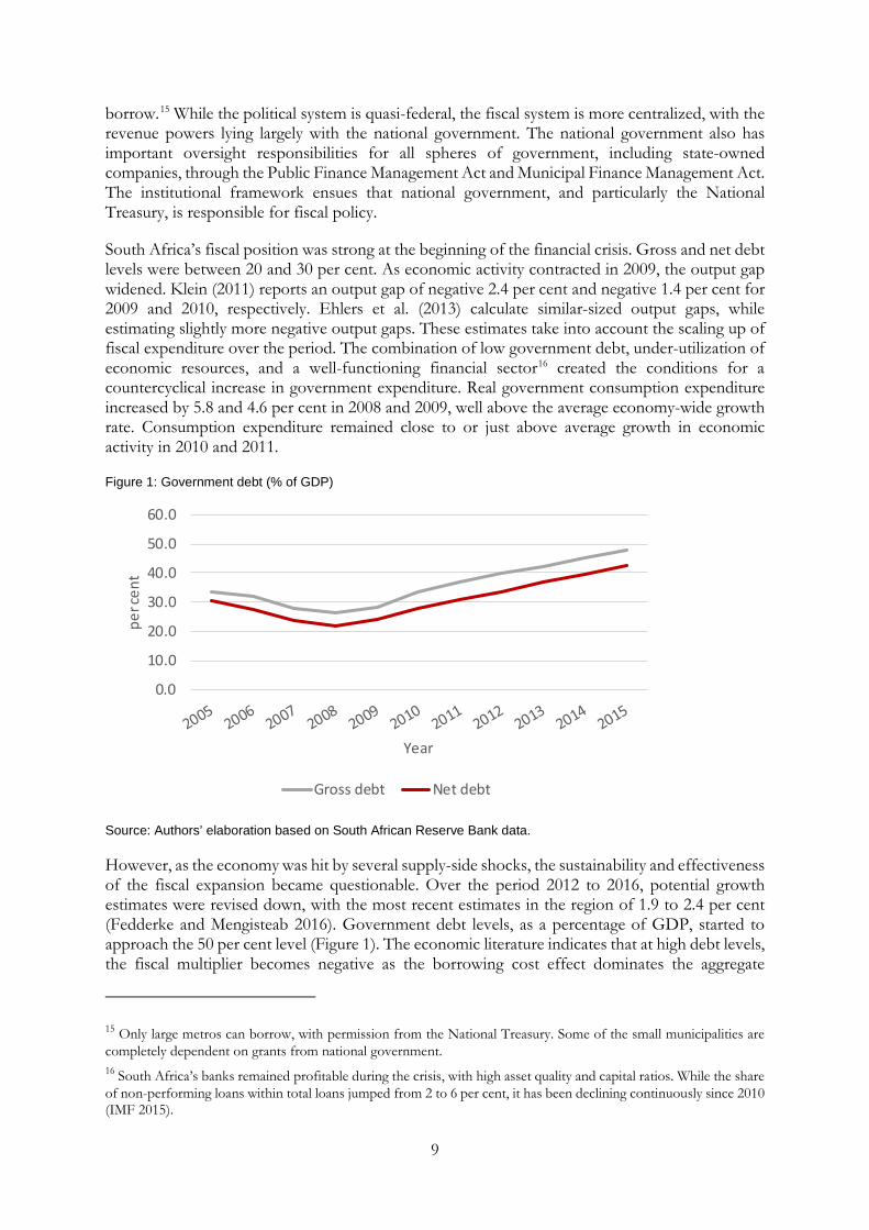
Figure 1: Government debt (% of GDP)

Source: Authors’ elaboration based on South African Reserve Bank data.

However, as the economy was hit by several supply-side shocks, the sustainability and effectiveness of the fiscal expansion became questionable. Over the period 2012 to 2016, potential growth estimates were revised down, with the most recent estimates in the region of 1.9 to 2.4 per cent (Fedderke and Mengisteab 2016). Government debt levels, as a percentage of GDP, started to approach the 50 per cent level (Figure 1). The economic literature indicates that at high debt levels, the fiscal multiplier becomes negative as the borrowing cost effect dominates the aggregate

15 Only large metros can borrow, with permission from the National Treasury. Some of the small municipalities are completely dependent on grants from national government. 16 South Africa’s banks remained profitable during the crisis, with high asset quality and capital ratios. While the share of non-performing loans within total loans jumped from 2 to 6 per cent, it has been declining continuously since 2010 (IMF 2015).

0.0

10.0

20.0

30.0

40.0

50.0

60.0

per c

ent

Year

Gross debt Net debt

10

demand impact of higher fiscal expenditure (Caner et al. 2010; Elmeskov and Sutherland 2012; Reinhart and Rogoff 2010). This channel requires the modelling of government debt balances and provides further support for the incorporation of stock-and-flow-consistent dynamics in our analysis. Concerns regarding the sustainability of government debt due to the threat of sovereign rating downgrade led to the implementation of spending ceilings, which were revised down in 2015 and 2016.

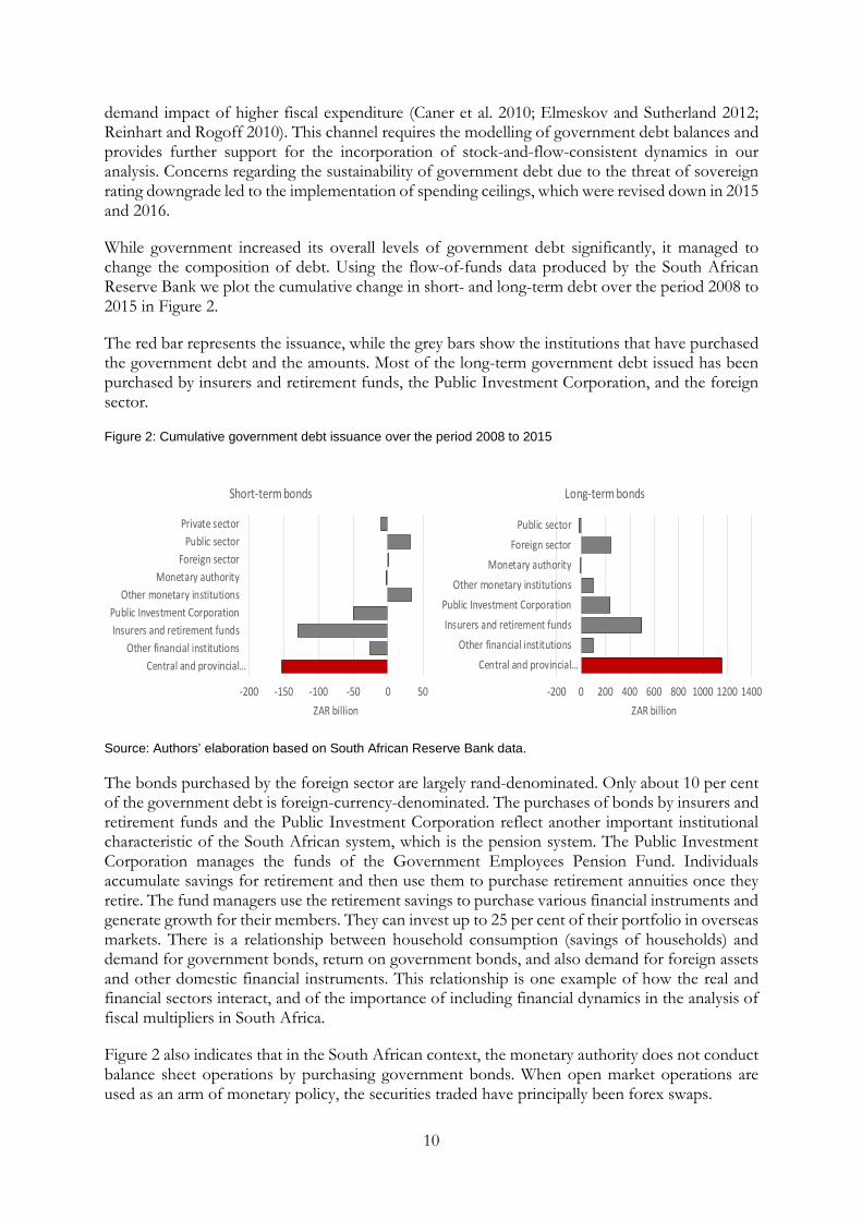
While government increased its overall levels of government debt significantly, it managed to change the composition of debt. Using the flow-of-funds data produced by the South African Reserve Bank we plot the cumulative change in short- and long-term debt over the period 2008 to 2015 in Figure 2.

The red bar represents the issuance, while the grey bars show the institutions that have purchased the government debt and the amounts. Most of the long-term government debt issued has been purchased by insurers and retirement funds, the Public Investment Corporation, and the foreign sector.

Figure 2: Cumulative government debt issuance over the period 2008 to 2015

Source: Authors’ elaboration based on South African Reserve Bank data.

The bonds purchased by the foreign sector are largely rand-denominated. Only about 10 per cent of the government debt is foreign-currency-denominated. The purchases of bonds by insurers and retirement funds and the Public Investment Corporation reflect another important institutional characteristic of the South African system, which is the pension system. The Public Investment Corporation manages the funds of the Government Employees Pension Fund. Individuals accumulate savings for retirement and then use them to purchase retirement annuities once they retire. The fund managers use the retirement savings to purchase various financial instruments and generate growth for their members. They can invest up to 25 per cent of their portfolio in overseas markets. There is a relationship between household consumption (savings of households) and demand for government bonds, return on government bonds, and also demand for foreign assets and other domestic financial instruments. This relationship is one example of how the real and financial sectors interact, and of the importance of including financial dynamics in the analysis of fiscal multipliers in South Africa.

Figure 2 also indicates that in the South African context, the monetary authority does not conduct balance sheet operations by purchasing government bonds. When open market operations are used as an arm of monetary policy, the securities traded have principally been forex swaps.

-200 0 200 400 600 800 1000 1200 1400

Central and provincial…Other financial institutions

Insurers and retirement fundsPublic Investment Corporation

Other monetary institutionsMonetary authority

Foreign sectorPublic sector

ZAR billion

Long-term bonds

-200 -150 -100 -50 0 50

Central and provincial…Other financial institutions

Insurers and retirement fundsPublic Investment Corporation

Other monetary institutionsMonetary authority

Foreign sectorPublic sector

Private sector

ZAR billion

Short-term bonds

11

4 Model changes and simulations

Makrelov et al. (2018) provide detailed description of the stock and flow model employed in this analysis. The model dynamics build on the simple computable general equilibrium model developed by Devarajan and Go (1998) and incorporate elements of DSGE models and stock and flow models in the tradition of Backus et al. (1980) and Godley and Lavoie (2012). The model also incorporates elements of the theoretical models developed by Borio and Zhu (2012) and Woodford (2010).

The stock and flow consistency of our framework implies that we have several financial instruments, rates of return, and institutional balance sheets. We model equities, bonds, loans, and cash and deposits as financial instruments; their returns; and the balance sheets of the Central Bank, the household sector, the financial sector, government, the non-financial sector, and the foreign sector. This is a significantly richer representation than the financial representation of institutions and financial instruments in DSGE models. The stock and flow consistency implies that there are strict budget constraints. Changes to the balance sheet of one institution must be matched by changes to the balance sheets of other institutions. Our approach to modelling household expectations is also different from that of current DSGE models. We aim to capture bounded rationality, which is supported by recent research on expectations (Hommes 2011; Roos and Luhan 2013).17

There are small changes to the model described in Makrelov et al. (2018) to reflect the conditions immediately after the 2008 crisis. We increase the responsiveness of price expectations in Equation 16 to the output gap. This implies that under a large negative output gap and with interest rates close to the lower effective bound, expectations are likely to be more responsive to changes in the output gap. This strengthens the mechanism identified by Christiano et al. (2011).

Prices and the repo rate, in Equations 11 and 34, respond only once the output gap turns positive. However, once the output gap becomes positive, the responses of prices and the repo rate in the model are stronger. This brings asymmetry into the model framework and creates dynamics which resemble zero lower bound conditions. Monetary policy accommodates expansionary fiscal policy as long as the output gap is negative. Equation 11 becomes

𝑃𝑃𝑃𝑃𝑡𝑡 = (1 + 𝑖𝑖𝑖𝑖𝑖𝑖) ∙ 𝑃𝑃𝑃𝑃𝑡𝑡−1 + 𝜃𝜃1𝑝𝑝𝑝𝑝_𝑝𝑝 ∙ �𝑦𝑦𝑡𝑡−1

𝑔𝑔𝑔𝑔𝑝𝑝𝑝𝑝,𝑙𝑙� + 𝜃𝜃2𝑝𝑝𝑝𝑝 ∙ ∆𝑃𝑃𝑃𝑃𝑡𝑡

where 𝜃𝜃1𝑝𝑝𝑝𝑝_𝑝𝑝 is larger than 𝜃𝜃1

𝑝𝑝𝑝𝑝 in the original model and 𝑦𝑦𝑡𝑡−1𝑔𝑔𝑔𝑔𝑝𝑝𝑝𝑝,𝑙𝑙 is 0 and becomes positive as the

proxy output gap variable becomes positive.

Equation 34 is now

𝑟𝑟𝑡𝑡𝑟𝑟𝑟𝑟𝑝𝑝𝑟𝑟 = 𝜌𝜌𝑟𝑟𝑟𝑟𝑝𝑝𝑟𝑟 ∙ 𝑟𝑟𝑡𝑡−1

𝑟𝑟𝑟𝑟𝑝𝑝𝑟𝑟 + (1 − 𝜌𝜌𝑟𝑟𝑟𝑟𝑝𝑝𝑟𝑟) ∙ �𝑖𝑖𝑖𝑖𝑖𝑖 + 𝛽𝛽2𝑟𝑟𝑟𝑟𝑝𝑝𝑟𝑟 ∙ (𝜋𝜋𝑡𝑡 − 𝑖𝑖𝑖𝑖𝑖𝑖� + 𝛽𝛽3

𝑟𝑟𝑟𝑟𝑝𝑝𝑟𝑟𝑝𝑝 ∙ (𝑦𝑦𝑡𝑡−1𝑔𝑔𝑔𝑔𝑝𝑝𝑝𝑝,𝑙𝑙))

where 𝛽𝛽3𝑟𝑟𝑟𝑟𝑝𝑝𝑟𝑟𝑝𝑝 is larger than 𝛽𝛽3

𝑟𝑟𝑟𝑟𝑝𝑝𝑟𝑟. Given that the repo rate and prices respond only to a positive output gap, these changes to the model amplify the positive impact on expected real rates because of an improvement in the output gap.

17 Bounded rationality originates in the work of Herbert Simon. For more information see Simon (1955, 1982, 1986).

12

Also, we introduce an additional term in the reserve ratio equation. The growth rate of savings affects the financial sector’s perceptions of risks. Higher growth compared with the baseline increases the ratio and thus reduces the money multiplier.

We impose a negative output gap on the model to reflect the conditions after the 2008 financial crisis. Using different methodologies for South Africa, Klein (2011) reports an output gap of negative 2.4 per cent and negative 1.4 per cent for 2009 and 2010 respectively. Ehlers et al. (2013) calculate similar-sized output gaps, while Anvari et al. (2014) estimate slightly more negative output gaps. We present two simulations:

a. A government expenditure shock of 1 per cent, which lasts over the entire period. In the first simulation, foreign savings are kept constant.

b. A government expenditure shock of 1 per cent, which lasts over the entire period, plus an increase in foreign savings inflows equivalent to 1 per cent of domestic savings.

All taxes are kept constant with government savings adjustments, which translates into an increased issuance of bonds.

5 Data

The construction of the data set and the calibration of the model also follow the approach outlined in Makrelov et al. (2018). We construct financial macro social accounting matrices (SAMs) for the South African economy over the period 2001 to 2012. Our approach follows the method outlined by Emini and Fofack (2003) and Hubic (2012). Capital and financial blocks are added to the standard SAM. These reflect the transactions that take place in the financial sector: the incurrence of liabilities and the accumulation of assets by institutions. The changes in liabilities and assets for a particular institution also reflect how the savings–investment balance (capital account) is financed.

The building of balance sheets for institutions relies on flow-of-funds data from 1970 onwards and the balance sheet information available in the Quarterly Bulletin published by the South African Reserve Bank. It is important to note that our institutional balance sheets deal only with financial instruments, as consistent data on ownership of non-financial assets and liabilities is not available. Thus, our balance sheets are partial but consistent when it comes to financial assets and liabilities.

The absence of separate price and quantity effects in the flow-of-funds data hinders the modelling of prices for financial instruments, particularly the prices of bonds and equities. We model only the equity price, which is based on the Johannesburg Stock Exchange All Share Index. The adjustment to the equity stocks follows the same approach as outlined by Aron and Muellbauer (2006). This adjustment leads to equity stock values which are more in line with the balance sheet information from the Quarterly Bulletin.

Other data on interest rates, growth rates, and price indices used in the calibration of the model are also sourced from the Reserve Bank’s Quarterly Bulletin.

6 Results

The results indicate the impact of government consumption expenditure under conditions of a large negative output gap, which persists over the period; a financial sector which remains sound;

13

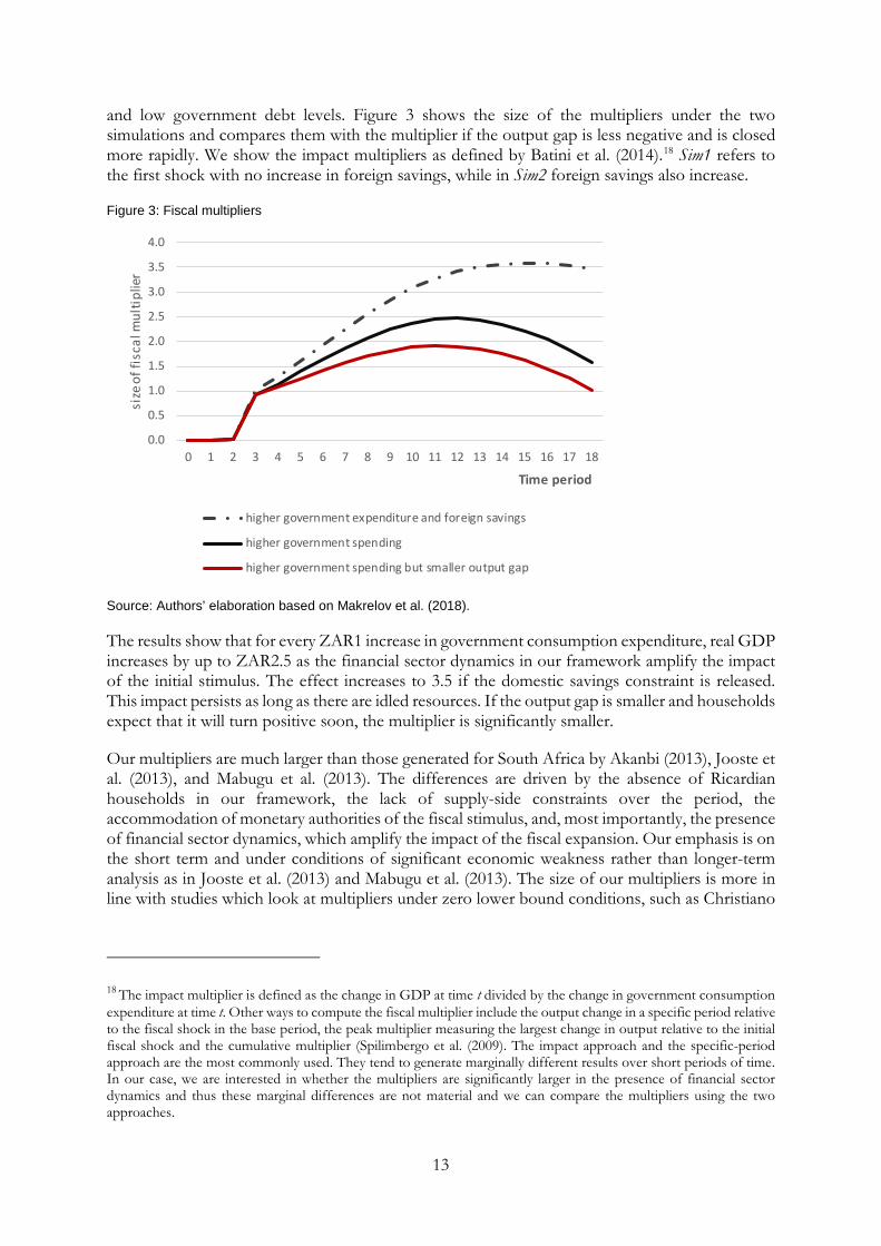
and low government debt levels. Figure 3 shows the size of the multipliers under the two simulations and compares them with the multiplier if the output gap is less negative and is closed more rapidly. We show the impact multipliers as defined by Batini et al. (2014).18 Sim1 refers to the first shock with no increase in foreign savings, while in Sim2 foreign savings also increase.

Figure 3: Fiscal multipliers

Source: Authors’ elaboration based on Makrelov et al. (2018).

The results show that for every ZAR1 increase in government consumption expenditure, real GDP increases by up to ZAR2.5 as the financial sector dynamics in our framework amplify the impact of the initial stimulus. The effect increases to 3.5 if the domestic savings constraint is released. This impact persists as long as there are idled resources. If the output gap is smaller and households expect that it will turn positive soon, the multiplier is significantly smaller.

Our multipliers are much larger than those generated for South Africa by Akanbi (2013), Jooste et al. (2013), and Mabugu et al. (2013). The differences are driven by the absence of Ricardian households in our framework, the lack of supply-side constraints over the period, the accommodation of monetary authorities of the fiscal stimulus, and, most importantly, the presence of financial sector dynamics, which amplify the impact of the fiscal expansion. Our emphasis is on the short term and under conditions of significant economic weakness rather than longer-term analysis as in Jooste et al. (2013) and Mabugu et al. (2013). The size of our multipliers is more in line with studies which look at multipliers under zero lower bound conditions, such as Christiano

18 The impact multiplier is defined as the change in GDP at time t divided by the change in government consumption expenditure at time t. Other ways to compute the fiscal multiplier include the output change in a specific period relative to the fiscal shock in the base period, the peak multiplier measuring the largest change in output relative to the initial fiscal shock and the cumulative multiplier (Spilimbergo et al. (2009). The impact approach and the specific-period approach are the most commonly used. They tend to generate marginally different results over short periods of time. In our case, we are interested in whether the multipliers are significantly larger in the presence of financial sector dynamics and thus these marginal differences are not material and we can compare the multipliers using the two approaches.

0.0

0.5

1.0

1.5

2.0

2.5

3.0

3.5

4.0

0 1 2 3 4 5 6 7 8 9 10 11 12 13 14 15 16 17 18

size

of f

isca

l mul

tiplie

r

Time period

higher government expenditure and foreign savings

higher government spending

higher government spending but smaller output gap

14

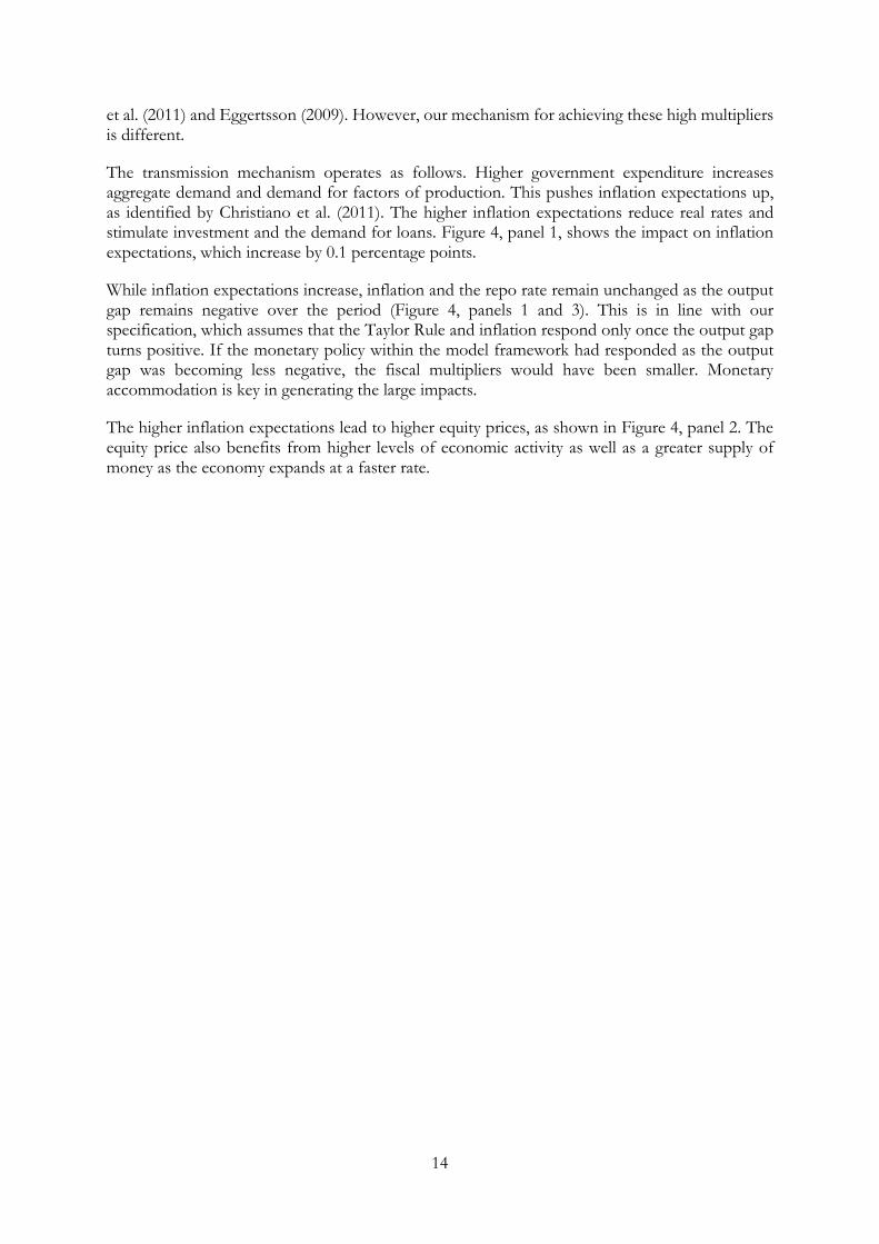
et al. (2011) and Eggertsson (2009). However, our mechanism for achieving these high multipliers is different.

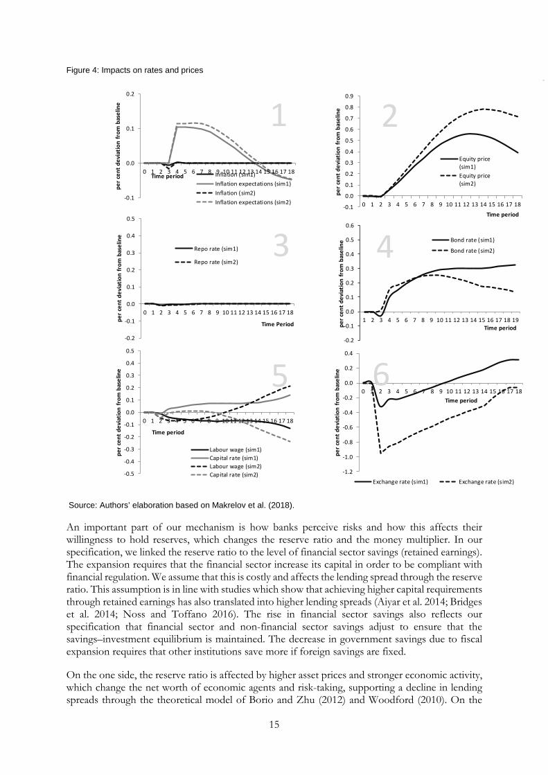
The transmission mechanism operates as follows. Higher government expenditure increases aggregate demand and demand for factors of production. This pushes inflation expectations up, as identified by Christiano et al. (2011). The higher inflation expectations reduce real rates and stimulate investment and the demand for loans. Figure 4, panel 1, shows the impact on inflation expectations, which increase by 0.1 percentage points.

While inflation expectations increase, inflation and the repo rate remain unchanged as the output gap remains negative over the period (Figure 4, panels 1 and 3). This is in line with our specification, which assumes that the Taylor Rule and inflation respond only once the output gap turns positive. If the monetary policy within the model framework had responded as the output gap was becoming less negative, the fiscal multipliers would have been smaller. Monetary accommodation is key in generating the large impacts.

The higher inflation expectations lead to higher equity prices, as shown in Figure 4, panel 2. The equity price also benefits from higher levels of economic activity as well as a greater supply of money as the economy expands at a faster rate.

15

Figure 4: Impacts on rates and prices

Source: Authors’ elaboration based on Makrelov et al. (2018).

An important part of our mechanism is how banks perceive risks and how this affects their willingness to hold reserves, which changes the reserve ratio and the money multiplier. In our specification, we linked the reserve ratio to the level of financial sector savings (retained earnings). The expansion requires that the financial sector increase its capital in order to be compliant with financial regulation. We assume that this is costly and affects the lending spread through the reserve ratio. This assumption is in line with studies which show that achieving higher capital requirements through retained earnings has also translated into higher lending spreads (Aiyar et al. 2014; Bridges et al. 2014; Noss and Toffano 2016). The rise in financial sector savings also reflects our specification that financial sector and non-financial sector savings adjust to ensure that the savings–investment equilibrium is maintained. The decrease in government savings due to fiscal expansion requires that other institutions save more if foreign savings are fixed.

On the one side, the reserve ratio is affected by higher asset prices and stronger economic activity, which change the net worth of economic agents and risk-taking, supporting a decline in lending spreads through the theoretical model of Borio and Zhu (2012) and Woodford (2010). On the

-0.1

0.0

0.1

0.2

0 1 2 3 4 5 6 7 8 9 10 11 12 13 14 15 16 17 18

per c

ent d

evia

tion

from

bas

elin

e

Time period Inflation (sim1)Inflation expectations (sim1)Inflation (sim2)Inflation expectations (sim2)

1

-0.1

0.0

0.1

0.2

0.3

0.4

0.5

0.6

0.7

0.8

0.9

0 1 2 3 4 5 6 7 8 9 10 11 12 13 14 15 16 17 18

per c

ent d

evia

tion

from

bas

elin

e

Time period

Equity price(sim1)Equity price(sim2)

2

-0.2

-0.1

0.0

0.1

0.2

0.3

0.4

0.5

0 1 2 3 4 5 6 7 8 9 10 11 12 13 14 15 16 17 18

per c

ent d

evia

tion

from

bas

elin

e

Time Period

Repo rate (sim1)

Repo rate (sim2)3

-0.2

-0.1

0.0

0.1

0.2

0.3

0.4

0.5

0.6

1 2 3 4 5 6 7 8 9 10 11 12 13 14 15 16 17 18 19

per c

ent d

evia

tion

from

bas

elin

e

Time period

Bond rate (sim1)

Bond rate (sim2)4

-0.5

-0.4

-0.3

-0.2

-0.1

0.0

0.1

0.2

0.3

0.4

0.5

0 1 2 3 4 5 6 7 8 9 10 11 12 13 14 15 16 17 18

per c

ent d

evia

tion

from

bas

elin

e

Time period

Labour wage (sim1)Capital rate (sim1)Labour wage (sim2)Capital rate (sim2)

5

-1.2

-1.0

-0.8

-0.6

-0.4

-0.2

0.0

0.2

0.4

0 1 2 3 4 5 6 7 8 9 10 11 12 13 14 15 16 17 18

per c

ent d

evia

tion

from

bas

elin

e

Time period

Exchange rate (sim1) Exchange rate (sim2)

6

16

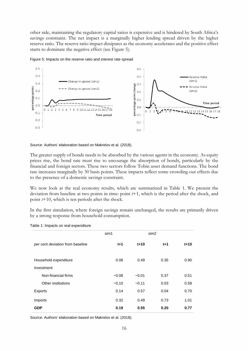
other side, maintaining the regulatory capital ratios is expensive and is hindered by South Africa’s savings constraint. The net impact is a marginally higher lending spread driven by the higher reserve ratio. The reserve ratio impact dissipates as the economy accelerates and the positive effect starts to dominate the negative effect (see Figure 5).

Figure 5: Impacts on the reserve ratio and interest rate spread

Source: Authors’ elaboration based on Makrelov et al. (2018).

The greater supply of bonds needs to be absorbed by the various agents in the economy. As equity prices rise, the bond rate must rise to encourage the absorption of bonds, particularly by the financial and foreign sectors. These two sectors follow Tobin asset demand functions. The bond rate increases marginally by 30 basis points. These impacts reflect some crowding-out effects due to the presence of a domestic savings constraint.

We now look at the real economy results, which are summarized in Table 1. We present the deviation from baseline at two points in time: point t+1, which is the period after the shock, and point t+10, which is ten periods after the shock.

In the first simulation, where foreign savings remain unchanged, the results are primarily driven by a strong response from household consumption.

Table 1: Impacts on real expenditure

sim1 sim2

per cent deviation from baseline t+1 t+10 t+1 t+10

Household expenditure 0.08 0.49 0.35 0.90

Investment

Non-financial firms −0.08 −0.01 0.37 0.51

Other institutions −0.10 −0.11 0.03 0.58

Exports 0.14 0.57 0.04 0.70

Imports 0.32 0.49 0.73 1.01

GDP 0.19 0.55 0.20 0.77

Source: Authors’ elaboration based on Makrelov et al. (2018).

17

Households see an increase in equity prices, higher flow of factor income, increase in the extension of loans, and somewhat lower dividend income due to higher levels of retained earnings by the financial and non-financial sectors. The increase in factor income from capital is driven by higher utilization leading to a higher capital rate. In the case of labour, employment increases, reducing the wage rate slightly. Based on their view of the economy, going ten periods ahead, households can afford to save less and consume more and still achieve their targeted level of wealth. This further exacerbates the savings constraint. Households effectively foresee the recovery in period t+10 at period t. The increase in the supply of loans is not driven by a lower reserve ratio but by a higher level of cash and deposits into the banking system as economic activity picks up. This allows for the supply of loans to increase.

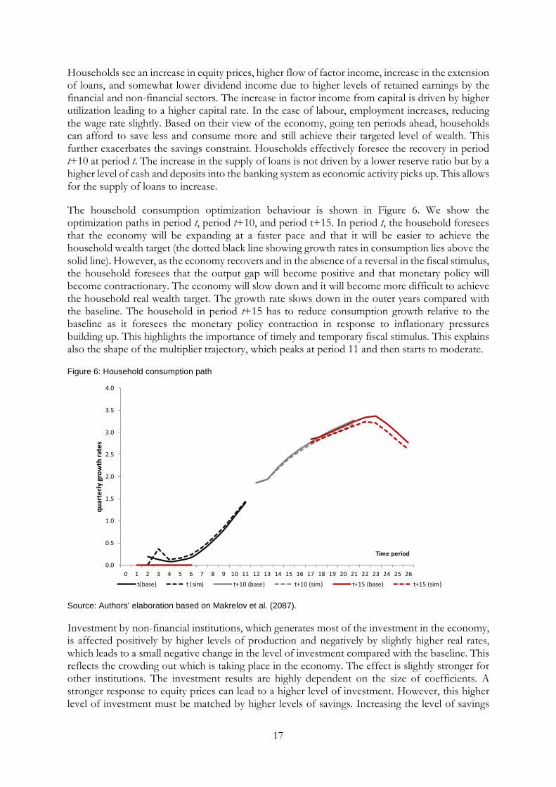
The household consumption optimization behaviour is shown in Figure 6. We show the optimization paths in period t, period t+10, and period t+15. In period t, the household foresees that the economy will be expanding at a faster pace and that it will be easier to achieve the household wealth target (the dotted black line showing growth rates in consumption lies above the solid line). However, as the economy recovers and in the absence of a reversal in the fiscal stimulus, the household foresees that the output gap will become positive and that monetary policy will become contractionary. The economy will slow down and it will become more difficult to achieve the household real wealth target. The growth rate slows down in the outer years compared with the baseline. The household in period t+15 has to reduce consumption growth relative to the baseline as it foresees the monetary policy contraction in response to inflationary pressures building up. This highlights the importance of timely and temporary fiscal stimulus. This explains also the shape of the multiplier trajectory, which peaks at period 11 and then starts to moderate.

Figure 6: Household consumption path

Source: Authors’ elaboration based on Makrelov et al. (2087).

Investment by non-financial institutions, which generates most of the investment in the economy, is affected positively by higher levels of production and negatively by slightly higher real rates, which leads to a small negative change in the level of investment compared with the baseline. This reflects the crowding out which is taking place in the economy. The effect is slightly stronger for other institutions. The investment results are highly dependent on the size of coefficients. A stronger response to equity prices can lead to a higher level of investment. However, this higher level of investment must be matched by higher levels of savings. Increasing the level of savings

0.0

0.5

1.0

1.5

2.0

2.5

3.0

3.5

4.0

0 1 2 3 4 5 6 7 8 9 10 11 12 13 14 15 16 17 18 19 20 21 22 23 24 25 26

quar

terly

gro

wth

rate

s

Time period

t(base) t (sim) t+10 (base) t+10 (sim) t+15 (base) t+15 (sim)

18

will require that the financial and non-financial sectors increase the level of retained earnings and decrease dividend payments. This also increases the loan spread, reflecting the shortage of savings in the domestic economy. There will be a short-term trade-off between household consumption and investment. However, a stronger response by investment changes the multiplier trajectory, as it expands production capacity. The recovery may be slower in the short run but the multiplier may be larger in the medium to long run.

Exports increase marginally in Table 1, which reflects the expansion in output. The exchange rate adjusts, given that foreign savings are fixed. Exports are fairly price-inelastic. Imports increase, as the currency is stronger in the short run and domestic demand increases. As the economy accelerates and dividend outflows increase, the currency depreciates. The depreciation supports export growth and makes imports more expensive.

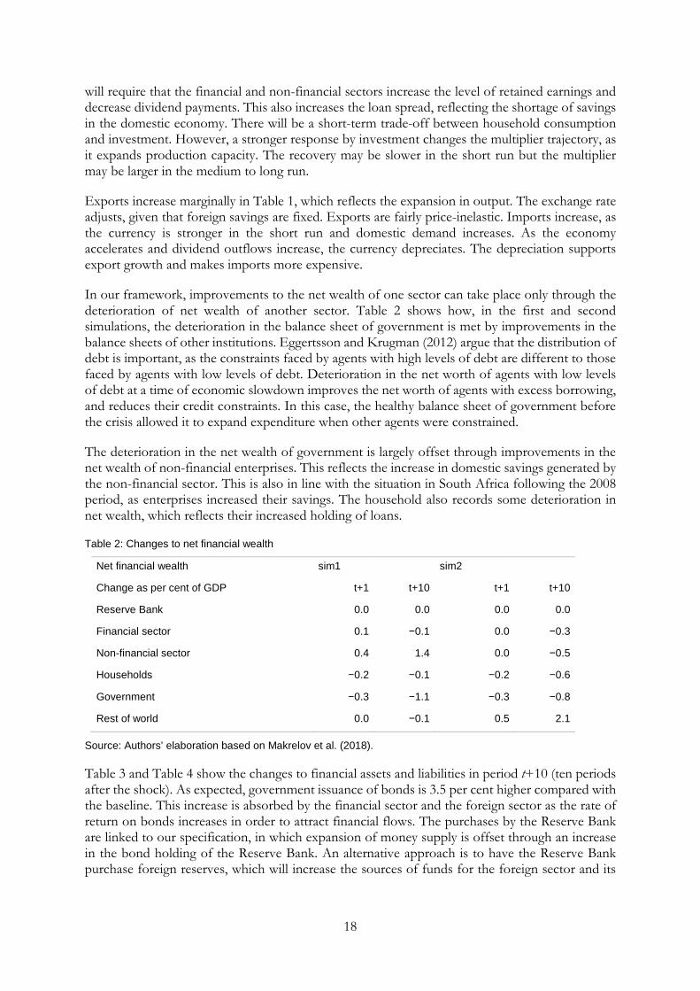
In our framework, improvements to the net wealth of one sector can take place only through the deterioration of net wealth of another sector. Table 2 shows how, in the first and second simulations, the deterioration in the balance sheet of government is met by improvements in the balance sheets of other institutions. Eggertsson and Krugman (2012) argue that the distribution of debt is important, as the constraints faced by agents with high levels of debt are different to those faced by agents with low levels of debt. Deterioration in the net worth of agents with low levels of debt at a time of economic slowdown improves the net worth of agents with excess borrowing, and reduces their credit constraints. In this case, the healthy balance sheet of government before the crisis allowed it to expand expenditure when other agents were constrained.

The deterioration in the net wealth of government is largely offset through improvements in the net wealth of non-financial enterprises. This reflects the increase in domestic savings generated by the non-financial sector. This is also in line with the situation in South Africa following the 2008 period, as enterprises increased their savings. The household also records some deterioration in net wealth, which reflects their increased holding of loans.

Table 2: Changes to net financial wealth

Net financial wealth sim1 sim2

Change as per cent of GDP t+1 t+10 t+1 t+10

Reserve Bank 0.0 0.0 0.0 0.0

Financial sector 0.1 −0.1 0.0 −0.3

Non-financial sector 0.4 1.4 0.0 −0.5

Households −0.2 −0.1 −0.2 −0.6

Government −0.3 −1.1 −0.3 −0.8

Rest of world 0.0 −0.1 0.5 2.1

Source: Authors’ elaboration based on Makrelov et al. (2018).

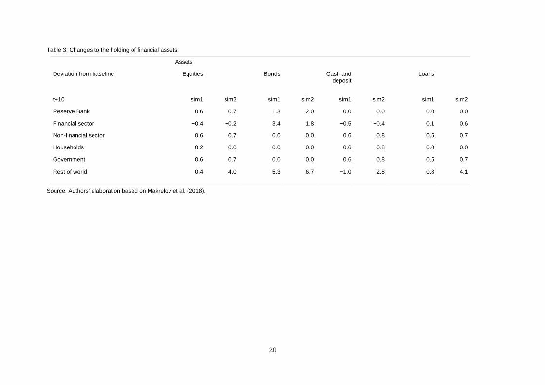
Table 3 and Table 4 show the changes to financial assets and liabilities in period t+10 (ten periods after the shock). As expected, government issuance of bonds is 3.5 per cent higher compared with the baseline. This increase is absorbed by the financial sector and the foreign sector as the rate of return on bonds increases in order to attract financial flows. The purchases by the Reserve Bank are linked to our specification, in which expansion of money supply is offset through an increase in the bond holding of the Reserve Bank. An alternative approach is to have the Reserve Bank purchase foreign reserves, which will increase the sources of funds for the foreign sector and its

19

purchases of bonds.19 If the bank also increases its purchases of bonds, this will absorb a greater share of the newly issued bonds, putting less pressure on bond yields while also increasing cash and deposits in circulation. This mechanism, which is considered unconventional monetary policy, will further amplify the positive effects associated with the fiscal expansion. The higher level of cash and deposits will increase the supply of loans and reduce the loan spread. At the same time, the financial and foreign sectors will invest more in assets other than government bonds, supporting asset prices and deposits with the financial sector. This will further strengthen the financial accelerator mechanism in our framework.

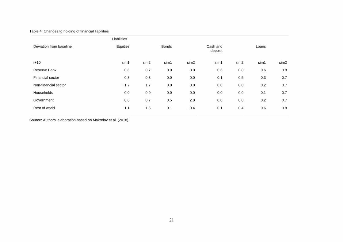
The increase in the equity holding of the Reserve Bank as an asset and liability reflects the higher equity price. We keep the quantity of equities held by the Reserve Bank constant. The Reserve Bank also increases money supply (cash and deposits) and its loan liability as economic activity accelerates.

The financial sector decreases its holding of equities and cash and deposits, as their relative return is lower than that of bonds. The growth in the liabilities of the financial sector reflects the higher levels of economic activity, which translate into higher levels of cash and deposits with the sectors as well as the higher equity prices and the increased holding of equities by the household sector. Our assumption is that the household equity assets are a liability of the financial sector balance sheet.20 The substitution away from cash and deposits for other assets through the Tobin asset demand function reduces the money creation process and slow down the financial accelerator process in our framework.

19 As indicated in Section 2, the South African Reserve Bank uses mostly currency swaps in its management of money supply so the current specification is a departure from the actual process. However, this is unlikely to change our overall result. 20 Most of the household equity holding is made up of interests in retirement and life funds, which we have classified as equities.

20

Table 3: Changes to the holding of financial assets

Assets

Deviation from baseline Equities Bonds Cash and deposit

Loans

t+10 sim1 sim2 sim1 sim2 sim1 sim2 sim1 sim2

Reserve Bank 0.6 0.7 1.3 2.0 0.0 0.0 0.0 0.0

Financial sector −0.4 −0.2 3.4 1.8 −0.5 −0.4 0.1 0.6

Non-financial sector 0.6 0.7 0.0 0.0 0.6 0.8 0.5 0.7

Households 0.2 0.0 0.0 0.0 0.6 0.8 0.0 0.0

Government 0.6 0.7 0.0 0.0 0.6 0.8 0.5 0.7

Rest of world 0.4 4.0 5.3 6.7 −1.0 2.8 0.8 4.1

Source: Authors’ elaboration based on Makrelov et al. (2018).

21

Table 4: Changes to holding of financial liabilities

Liabilities

Deviation from baseline Equities Bonds Cash and deposit

Loans

t+10 sim1 sim2 sim1 sim2 sim1 sim2 sim1 sim2

Reserve Bank 0.6 0.7 0.0 0.0 0.6 0.8 0.6 0.8

Financial sector 0.3 0.3 0.0 0.0 0.1 0.5 0.3 0.7

Non-financial sector −1.7 1.7 0.0 0.0 0.0 0.0 0.2 0.7

Households 0.0 0.0 0.0 0.0 0.0 0.0 0.1 0.7

Government 0.6 0.7 3.5 2.8 0.0 0.0 0.2 0.7

Rest of world 1.1 1.5 0.1 −0.4 0.1 −0.4 0.6 0.8

Source: Authors’ elaboration based on Makrelov et al. (2018).

22

Similarly, the foreign sector decreases its holding of cash and deposits relative to the baseline. The higher financial wealth of the foreign sector is driven not by an increase in net savings, but by the higher equity prices and an increase in the value of equity and loan liabilities as the economy grows faster and domestic residents invest abroad.

The household, whose asset demand is linked to its level of nominal income, increases its holdings of equities and cash deposits. The increase in the equity holding also reflects the higher equity price. The household does not provide loans, and our assumption is that it does not demand bonds due to its small holding in the underlying data. Some of the increase in the household financial wealth is financed through an increase in the holding of loans and some reflects the higher equity price.

The equity liability of the non-financial sector declines relative to the baseline, which reflects the fall in demand for equities by the financial sector. The non-financial sector provides equities to ensure that the balance between supply and demand is satisfied. Despite the fall in its ability to fund financial wealth through equity sales, financial wealth for the sector increases. This is due to an increase in equity prices, loans taken by the sector, and net savings. The holdings of assets in the form of equities, loans, and cash and deposits are around 0.6 per cent higher than in the baseline. The provision of loans by the financial sector is linked to the level of financial wealth: the higher the wealth, the more loans are extended. These are generally in the form of trade loans. We assume that non-financial institutions do not demand government bonds as they have a very small holding in the data used for the calibration.

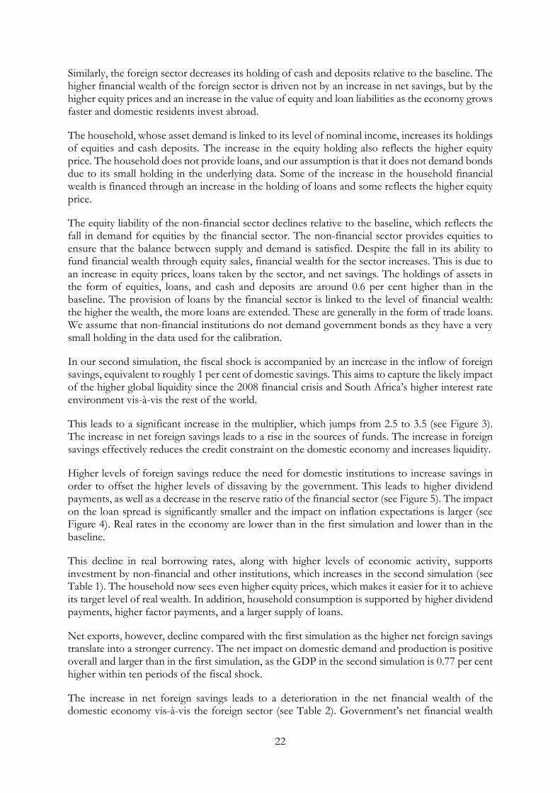
In our second simulation, the fiscal shock is accompanied by an increase in the inflow of foreign savings, equivalent to roughly 1 per cent of domestic savings. This aims to capture the likely impact of the higher global liquidity since the 2008 financial crisis and South Africa’s higher interest rate environment vis-à-vis the rest of the world.

This leads to a significant increase in the multiplier, which jumps from 2.5 to 3.5 (see Figure 3). The increase in net foreign savings leads to a rise in the sources of funds. The increase in foreign savings effectively reduces the credit constraint on the domestic economy and increases liquidity.

Higher levels of foreign savings reduce the need for domestic institutions to increase savings in order to offset the higher levels of dissaving by the government. This leads to higher dividend payments, as well as a decrease in the reserve ratio of the financial sector (see Figure 5). The impact on the loan spread is significantly smaller and the impact on inflation expectations is larger (see Figure 4). Real rates in the economy are lower than in the first simulation and lower than in the baseline.

This decline in real borrowing rates, along with higher levels of economic activity, supports investment by non-financial and other institutions, which increases in the second simulation (see Table 1). The household now sees even higher equity prices, which makes it easier for it to achieve its target level of real wealth. In addition, household consumption is supported by higher dividend payments, higher factor payments, and a larger supply of loans.

Net exports, however, decline compared with the first simulation as the higher net foreign savings translate into a stronger currency. The net impact on domestic demand and production is positive overall and larger than in the first simulation, as the GDP in the second simulation is 0.77 per cent higher within ten periods of the fiscal shock.

The increase in net foreign savings leads to a deterioration in the net financial wealth of the domestic economy vis-à-vis the foreign sector (see Table 2). Government’s net financial wealth

23

declines by less compared with the first simulation, driven by stronger revenue growth in the second simulation.

All institutions increase their holdings of loans by more than in the first simulation, driven by the lower real rates and stronger growth in the domestic economy.

The higher bond supply is now absorbed mainly by the foreign sector, while the financial sector absorbs less compared with the first simulation, as the relative return of bonds is smaller. The Reserve Bank’s increase in bond holdings is related to the increased supply of money.

The reduction in the reserve ratio, which reflects reduction in risk perceptions and higher valuation but also reduction in the domestic savings constraint, leads to an increase in the supply of loans relative to the baseline and the first simulation. Lending is also supported by stronger growth of deposits with the financial sector. Equities and cash and deposit assets of the financial sector still decline marginally, as the relative return of bonds is still more favourable.

The asset accumulation of the foreign sector increases across asset classes, as the sector now also benefits from an increase in net savings as a source of funding relative to the first simulation. The bond and cash and deposit liability of the foreign sector falls, which reflects the stronger currency. We assume that bond and cash liabilities for the foreign sector are fixed in foreign currency units. The equity and bond liabilities increase as the stronger domestic growth and currency encourage domestic residences to diversify their portfolio and invest abroad.21

The higher demand for equities and the higher price lead to a larger increase in the equity liability of the foreign sector.

Our result, that the fiscal multiplier increases substantially with an increase in net foreign savings, somewhat contradicts studies that argue that the fiscal multiplier tends to be lower in more open economies due to import leakage (Ilzetzki et al. 2013; Jooste et al. 2013). While imports subtract from GDP, foreign savings can reduce domestic credit constraints and support the financial accelerator mechanism in the presence of spare capacity in the domestic economy. Our results support the findings of Blanchard et al. (2016) that inflows can be expansionary. In our framework, however, the mechanism works through the impact on equity prices, spreads, and the balance sheets of all institutions in the economy, particularly the household and financial sectors. These work together to amplify the effects of the original fiscal shock.

Finally, in Figure 3 we show the impact on the fiscal multiplier if the output gap is less negative. The red and black lines move together initially. The household foresees now that the output gap will be closed faster and inflation will start rising, leading to an increase in the policy rate. It will be more difficult to achieve its real level of targeted wealth. The household needs to save more and consume less.

In the absence of a negative output gap, the multiplier would have been negative, as monetary policy responds immediately to reduce inflation by increasing the repo rate. The effect depends on the parameters in the Taylor Rule, but also on the parameters in the equation for the financial sector reserve ratio. A lower value of 𝛽𝛽𝑟𝑟𝑟𝑟𝑝𝑝𝑟𝑟 will reduce the impact of monetary policy on the financial sector and reduce the negative impact.

21 In our specification, equity and bond liabilities of the foreign sector are driven by the domestic GDP expressed in foreign currency units.

24

South Africa’s fiscal expansion could be financed easily because government finances were perceived as sustainable due to the low debt-to-GDP ratio at the time of the fiscal expansion, and the financial sector could intermediate between the purchasers of bonds and the government. If the financial sector had been under stress and unable to intermediate, even in the presence of sustainable government finances, the state would have not been able to fund its expenditure and the financial accelerator effect would not have been operational. The reserve ratio in our model would be very high and the financial sector would transform its financial wealth not into loans but into cash and deposits. Under extreme financial stress, the financial sector inability to purchase government bonds would require the Reserve Bank to intervene and purchase the bonds. In this case, the fiscal expansion would be reduced to unconventional monetary policy (Borio and Disyatat 2010).

7 Conclusion

Our main conclusion is that financial sector dynamics have an important role to play in amplifying the impact of fiscal expansion under conditions characterized by large negative output gaps. The transmission mechanism works through the real lending spread over the deposit rate, asset prices, and balance sheets of all institutions in the economy, which amplify the initial fiscal shock. The sources and uses of funds are interlinked in our framework and work together to generate a financial accelerator mechanism. The balance sheets of households and the financial sector play particularly important roles. Household consumption depends on the ability of households to achieve their target level of wealth. An important part of our mechanism is the willingness of banks to hold reserves in order to manage regulatory requirements, but also risk. Following the theoretical models of Borio and Zhu (2012) and Woodford (2010), improvements in economic activity reduce risk perception and improve valuations, making it easier for banks to achieve their capital requirements, which translates into higher lending. This in turn supports further expansion in output, creating a feedback mechanism. Our results indicate that South Africa’s savings constraint limits the operations of this mechanism.

Improvements in the net worth of agents with high levels of debt can increase the money multiplier and reduce credit constraints. This requires, however, a fall in the net worth of agents with low debt. Our framework allows us to trace precisely changes in flows and stocks and identify the impact of policy decisions on the balance sheets of all agents in the economy.

In terms of policy, our results indicate that policymakers need to have knowledge not only of the size of the output gap but also of the health of the financial sector, its perceptions of risk, and the likely impact of its decisions on economic agents, particularly those with high debt levels. The Reserve Bank has an important role to play, particularly if the ability of the financial sector to intermediate is being hindered. It can also reduce the impact on bond rates and improve the sustainability of the fiscal expansion if it purchases more bonds, increasing the supply of money and reducing bond yields and asset substitution. This constitutes unconventional monetary policy.

The inflow of foreign savings in the period immediately after the 2008 financial crisis supported the fiscal expansion and led to higher fiscal multipliers by reducing the savings constraint in the economy and increasing the sources of funding. These inflows reflected monetary policy interventions in advanced economies, but also the macroeconomic stability of the domestic economy. The impact of domestic policy interventions was influenced by policy developments in the global economy. In a savings-constraint economy, such as that of South Africa, monetary and fiscal policy need to pay particular attention to the inflow of foreign savings as this can be expansionary, as pointed out by Blanchard et al. (2016). This requires the rethinking of the

25

execution and co-ordination of domestic macroeconomic policies, as well as their co-ordination with macroeconomic policy globally.

References

Afonso, A., and R.M. Sousa (2012). ‘The Macroeconomic Effects of Fiscal Policy’. Applied Economics, 44: 4439–54.

Afonso, A., J. Baxa, and M. Slavik (2011). ‘Fiscal Developments and Financial Stress: A Threshold VAR Analysis’. European Central Bank Working Paper Series 1319. Frankfurt am Main: European Central Bank.

Agnello, L., and R.M. Sousa (2013). ‘Fiscal Policy and Asset Prices’. Bulletin of Economic Research, 65: 154–77.

Aiyar, S., C.W. Calomiris, J. Hooley, Y. Korniyenko, and T. Wieladek (2014). ‘The International Transmission of Bank Capital Requirements: Evidence from the UK’. Journal of Financial Economics, 113: 368–82.

Akanbi, O.A. (2013). ‘Macroeconomic Effects of Fiscal Policy Changes: A Case of South Africa’. Economic Modelling, 35: 771–85.

Anvari, V., N. Ehlers, and R. Steinbach (2014). ‘A Semi-Structural Approach to Estimate South Africa’s Potential Output’. South African Reserve Bank Working Paper Series 8. Pretoria: South African Reserve Bank.

Aron, J., and J. Muellbauer (2006). ‘Estimates of Household Sector Wealth for South Africa, 1970–2003’. Review of Income and Wealth, 52: 285–307.

Auerbach, A.J., and Y. Gorodnichenko (2012). ‘Measuring the Output Responses to Fiscal Policy’. American Economic Journal: Economic Policy, 4: 1–27.

Backus, D., W. Brainard, G. Smith, and J. Tobin (1980). ‘A Model of U.S. Financial and Nonfinancial Economic Behavior’. Journal of Money, Credit, and Banking, 12: 259–93.

Bank for International Settlements (2016). Triennial Central Bank Survey: Foreign Exchange Turnover in April 2016. Basel: Monetary and Economic Department, Bank for International Settlements. Available at: http://www.bis.org/publ/rpfx16fx.pdf (accessed 1 August 2016).

Batini, N., L. Eyraud, and A. Weber (2014). ‘A Simple Method to Compute Fiscal Multipliers’. Working Paper 14/93. Washington, DC: International Monetary Fund.

BCBS (Basel Committee on Banking Supervision) (2011). ‘The Transmission Channels between the Financial and Real Sectors: A Critical Survey of the Literature’. Working Paper 18. Basel: Bank for International Settlements.

Bernanke, B.S., M. Gertler, and S. Gilchrist (1999). ‘The Financial Accelerator in a Quantitative Business Cycle Framework’. In J.B. Taylor and M. Woodford (eds), Handbook of macroeconomics. Volume 1C. Amsterdam, New York, and Oxford: Elsevier Science, North-Holland.

Blanchard, O.J., and D. Leigh (2014). ‘Learning about Fiscal Multipliers from Growth Forecast Errors’. IMF Economic Review, 62: 179–212.

Blanchard, O., J.D. Ostry, A.R. Ghosh, and M. Chamon (2016). ‘Do Capital Flows Need To Be Tamed? Capital Flows: Expansionary or Contractionary?’. The American Economic Review, 106: 565–69.

26

Borio, C., and P. Disyatat (2010). ‘Unconventional Monetary Policies: An Appraisal’. The Manchester School, 78(s1): 53–89.

Borio, C., and H. Zhu (2012). ‘Capital Regulation, Risk-Taking and Monetary Policy: A Missing Link in the Transmission Mechanism?’ Journal of Financial Stability, 8: 236–51.

Bridges, J., D. Gregory, M. Nielsen, S. Pezzini, A. Radia, and M. Spaltro (2014). ‘The Impact of Capital Requirements on Bank Lending’. Working Paper 486. London: Bank of England.

Caner, M., T. Grennes, and F. Koehler-Geib (2010). ‘Finding the Tipping Point: When Sovereign Debt Turns Bad’. Policy Research Working Paper 5391. Washington, DC: World Bank.

Carlin, W., and D.W. Soskice (2015). Macroeconomics: Institutions, Instability, and the Financial System. Oxford: Oxford University Press.

Carrillo, J.A., and C. Poilly (2010). ‘On the Recovery Path during a Liquidity Trap: Do Financial Frictions Matter for Fiscal Multipliers?’ IRES Discussion Paper 2010034. Louvain-la-Neuve: Institut de Recherches Economiques et Sociales, Universitè catholique de Louvain.

Christiano, L.J., M. Eichenbaum, and C.L. Evans (2005). ‘Nominal Rigidities and the Dynamic Effects of a Shock to Monetary Policy’. Journal of Political Economy, 113: 1–45.

Christiano, L., M. Eichenbaum., and S. Rebelo (2011). ‘When Is the Government Spending Multiplier Large?’ Journal of Political Economy, 119: 78–121.

Coenen, G. (2012). ‘Effects of Fiscal Stimulus in Structural Models’. American Economic Journal: Macroeconomics, 4: 22–68.

Cogan, J.F., T. Cwik, J.B. Taylor, and V. Wieland (2010). ‘New Keynesian versus Old Keynesian Government Spending Multipliers’. Journal of Economic Dynamics and Control, 34: 281–95.

Delong, J.B., L.H. Summers, M. Feldstein, and V.A. Ramey (2012). ‘Fiscal Policy in a Depressed Economy [with Comments and Discussion]’. Brookings Papers on Economic Activity, Spring: 233–97.

Devarajan, S., and D.S. Go (1998). ‘The Simplest Dynamic General-Equilibrium Model of an Open Economy’. Journal of Policy Modeling, 20: 677–714.

Eggertsson, G.B. (2009). ‘What Fiscal Policy Is Effective at Zero Interest Rates?’ Staff Report 402. New York: Federal Reserve Bank.

Eggertsson, G.B., and P. Krugman (2012). ‘Debt, Deleveraging, and the Liquidity Trap: A Fisher-Minsky-Koo Approach’. Quarterly Journal of Economics, 127: 1469–513.

Ehlers, N., L. Mboji, and M. Smal (2013). ‘The Pace of Potential Output Growth in the South African Economy’. Working Paper 1. Pretoria: South African Reserve Bank.

Elmeskov, J., and D. Sutherland (2012). ‘Post-Crisis Debt Overhang: Growth and Implications across Countries’. Mimeo. Paris: Economics Department, OECD.

Emini, C.A., and H. Fofack (2003). A Financial Social Accounting Matrix for the Integrated Macroeconomic Model for Poverty Analysis: Application to Cameroon with a Fixed-Price Multiplier Analysis. Washington, DC: World Bank Publications.

Fazzari, S.M., J. Morley, and I. Panovska (2015). ‘State-Dependent Effects of Fiscal Policy’. Studies in Nonlinear Dynamics and Econometrics, 19: 285–315.

Fedderke, J.W., and D.K. Mengisteab (2016). ‘Estimating South Africa’s Output Gap Potential Growth Rate’. Working Paper 16/02. Pretoria: South African Reserve Bank.

Fernández-Villaverde, J. (2010). ‘Fiscal Policy in a Model With Financial Frictions’. The American Economic Review, 100: 35–40.

27

Gali, J., J.D. Lopez-Salido, and J. Valles (2007). ‘Understanding the Effects of Government Spending on Consumption’. Journal of the European Economic Association, 5: 227–70.

Gertler, M., and P. Karadi (2011). ‘A Model of Unconventional Monetary Policy’. Journal of Monetary Economics, 58: 17–34.

Gertler, M., N. Kiyotaki, and A. Queralto (2012). ‘Financial Crises, Bank Risk Exposure and Government Financial Policy’. Journal of Monetary Economics, 59(Supplement): S17–S34.

Godley, W., and M. Lavoie (2007). Monetary Economics: An Integrated Approach to Credit, Money, Income, Production and Wealth. Houndmills and New York: Palgrave Macmillan.

Godley, W., and M. Lavoie (2012). Monetary Economics: An Integrated Approach to Credit, Money, Income, Production and Wealth. New York: Springer.

Hommes, C. (2011). ‘The Heterogeneous Expectations Hypothesis: Some Evidence from the Lab’. Journal of Economic Dynamics and Control, 35: 1–24.

Hubic, A. (2012). ‘A Financial Social Accounting Matrix (SAM) for Luxembourg’. BCL Working Paper 72. Luxembourg: Central Bank of Luxembourg.

Huidrom, R., A. Kose, J.J. Lim, and F. Ohnsorge (2016). ‘Do Fiscal Multipliers Depend on Fiscal Positions?’ Policy Research Working Paper 7724. Washington, DC: World Bank.

Hur, S.-K., S. Mallick, and D. Park (2014). ‘Fiscal Policy and Crowding Out in Developing Asia’. Environment and Planning C: Government and Policy, 32: 1117–32.

Ilzetzki, E., E.G. Mendoza, and C.A. Vegh (2013). ‘How Big (Small?) Are Fiscal Multipliers?’ Journal of Monetary Economics, 60: 239–54.

IMF (2015). ‘Detailed Assesment of Copliance on the Basel Core Principles for Effective Banking Supervision’. Country Report 15/55. Washington, DC: International Monetary Fund.

Jawadi, F., S.K. Mallick, and R.M. Sousa (2014). ‘Fiscal Policy in the BRICs’. Studies in Nonlinear Dynamics and Econometrics, 18: 201–15.

Jha, S., S.K. Mallick, D. Park, and P.F. Quising (2014). ‘Effectiveness of Countercyclical Fiscal Policy: Evidence from Developing Asia’. Journal of Macroeconomics, 40: 82–98.

Jooste, C., G. Liu, and R. Naraidoo (2013). ‘Analysing the Effects of Fiscal Policy Shocks in the South African Economy’. Economic Modelling, 32: 215–24.

Klein, N. (2011). ‘Measuring the Potential Output of South Africa’. African Departmental Paper 11/2. Washington, DC: International Monetary Fund.

Kollmann, R., M. Ratto, W. Roeger, and J. in’t Veld (2013). ‘Fiscal Policy, Banks and the Financial Crisis’. Journal of Economic Dynamics and Control, 37: 387–403.

Mabugu, R., V. Robichaud, H. Maisonnave, and M. Chitiga (2013). ‘Impact of Fiscal Policy in an Intertemporal CGE Model for South Africa’. Economic Modelling, 31: 775–82.

Makrelov, K., C. Arndt, R. Davies, and L. Harris (2018). ‘Stock-and-Flow-Consistent Macroeconomic Model for South Africa’. Working Paper 2018/007. Helsinki: UNU-WIDER.

Merola, R.. (2012). ‘Monetary Policy and Fiscal Stimulus with the Zero Lower Bound and Financial Frictions’. IRES Discussion Paper 2012-24. Louvain-la-Neuve: Institut de Recherches Economiques et Sociales, Universitè catholique de Louvain.

Mineshima, A., M. Poplawski-Ribeiro, and A. Weber (2014). ‘Size of Fiscal Multipliers’. In C. Cottarelli, P. Gerson, and A. Senhadji (eds), Post-Crisis Fiscal Policy. Cambridge, MA: MIT Press.

28

Mittnik, S., and W. Semmler (2013). ‘The Real Consequences of Financial Stress’. Journal of Economic Dynamics and Control, 37: 1479–99.

Nickel, C., and A. Tudyka (2014). ‘Fiscal Stimulus in Times of High Debt: Reconsidering Multipliers and Twin Deficits’. Journal of Money, Credit, and Banking, 46: 1313–44.

Noss, J., and P. Toffano (2016). ‘Estimating the Impact of Changes in Aggregate Bank Capital Requirements on Lending and Growth during an Upswing’. Journal of Banking & Finance, 62: 15–27.

Owyang, M.T., V.A. Ramey, and S. Zubairy (2013). ‘Are Government Spending Multipliers Greater during Periods of Slack? Evidence from Twentieth-Century Historical Data’. American Economic Review, 103: 129–34.

Proaño, C.R., C. Schoder, and W. Semmler (2014). ‘Financial Stress, Sovereign Debt and Economic Activity in Industrialized Countries: Evidence from Dynamic Threshold Regressions’. Journal of International Money and Finance, 45: 17–37.

Reinhart, C.M., and K.S. Rogoff (2009). ‘The Aftermath of Financial Crises’. American Economic Review, 99: 466–72.

Reinhart, C.M., and K.S. Rogoff (2010). ‘Growth in a Time of Debt’. American Economic Review, 100: 573–78.

Rey, H. (2015). ‘Dilemma not Trilemma: The Global Financial Cycle and Monetary Policy Independence’. NBER Working Papers 21162. Cambridge, MA: National Bureau of Economic Research.

Riera-Crichton, D., C.A. Vegh, and G. Vuletin (2015). ‘Procyclical and Countercyclical Fiscal Multipliers: Evidence from OECD Countries’. Journal of International Money and Finance, 52: 15–31.

Roos, M.W.M., and W.J. Luhan (2013). ‘Information, Learning and Expectations in an Experimental Model Economy’. Economica, 80: 513–31.

Simon, H.A. (1955). ‘A Behavioral Model of Rational Choice’. The Quarterly Journal of Economics, 69: 99–118.

Simon, H.A. (1982). Models of Bounded Rationality: Empirically Grounded Economic Reason. Cambridge, MA: MIT Press.

Simon, H.A. (1986). ‘Rationality in Psychology and Economics’. The Journal of Business, 59: S209–S24.

Smets, F., and R. Wouters (2007). ‘Shocks and Frictions in US Business Cycles: A Bayesian DSGE Approach’. American Economic Review, 97: 586–606.

Spilimbergo, A., M. Schindler, and S.A. Symansky (2009). Fiscal Multipliers. Staff Position Note SPN/09/11. Washington, DC: International Monetary Fund.

Tobin, J. (1982). ‘Money and Finance in the Macroeconomic Process’. Journal of Money, Credit & Banking, 14: 171–204.

Woodford, M. (2010). ‘Financial Intermediation and Macroeconomic Analysis’. Journal of Economic Perspectives, 24: 21–44.