Working Paper Series7/2018

ALTERNATIVE FRAMEWORKS FOR MEASURING CREDIT GAPS AND SETTING COUNTERCYCLICAL CAPITAL BUFFERS

NICOLAS REIGLLENNO UUSKÜLA

The Working Paper is available on the Eesti Pank web site at:http://www.eestipank.ee/en/publications/series/working-papers

For information about subscription call: +372 668 0998; Fax: +372 668 0954e-mail: publications@eestipank.ee

DOI: 10.23656/25045520/072018/0159

ISBN 978-9949-606-44-3 (hard copy)ISBN 978-9949-606-43-6 (pdf)

Eesti Pank. Working Paper Series, ISSN 1406-7161; 7/2018 (hard copy)Eesti Pank. Working Paper Series, ISSN 2504-5520; 7/2018 (pdf)

1

Alternative frameworks for measuring credit gaps and

setting countercyclical capital buffers

Nicolas Reigl and Lenno Uusküla*

Abstract

This paper complements the standard Basel countercyclical capital buffer

framework by suggesting four additional measures for credit gaps that can be used to measure the financial cycle and to decide on countercyclical capital buffers for banks. The new measures behave similarly to the gaps calculated with the standard Basel one-sided Hodrick-Prescott filter in long samples, but they have the properties desired for countries with relatively short historical samples. While the standard Basel credit gaps have been deep in negative territory for many European Union countries since the Great Recession the new gaps are close to zero and the buffers suggested are more in line with the countercyclical capital buffer ratios that were in place in 2018.

JEL Codes: G01, E59

Keywords: credit gaps, countercyclical capital buffer, Basel III, Estonia

The views expressed are those of the author and do not necessarily represent the official views of Eesti Pank, the European Central Bank or the Eurosystem.

* Nicolas Reigl (Eesti Pank. Email: nicolas.reigl@eestipank.ee), Lenno Uusküla (corresponding author, Eesti

Pank, Email: lenno.uuskyla@eestipank.ee). We thank for valuable comments from Silver Karolin, Jana Kask, Timo Kosenko, Martti Randveer, Tairi Rõõm, Mari Tamm and participants at the Eesti Pank seminar and the Baltic Central Bank meeting.

2

Non-technical summary

The Basel III framework requires positive countercyclical capital buffers to be set for banks when credit is growing excessively and released when the financial cycle turns. The credit gap, the key indicator for the buffer, is measured by comparing the debt-to-GDP ratio to its trend value, which is calculated with a particular one-sided Hodrick-Prescott filter. For Estonia and many other European Union countries this approach leaves the credit gap deep in negative territory in 2018. When the debt and GDP forecasts of Eesti Pank are used, the approach predicts a negative gap up until 2025.

This paper evaluates alternative approaches for calculating periods of excessive credit growth when countercyclical capital buffers should be set. It suggests four additional measures for credit gaps: the change in the credit-to-GDP ratio over two years; the growth in credit compared to the eight-year moving average of growth in nominal GDP over two years; the growth in credit compared to annual nominal growth of 5% over two years; and growth in credit relative to the nominal GDP trend value over two years. Buffer rates can be set following the original Basel suggestions for all the proposed new measures.

3

Contents

1. Introduction ............................................................................................................................ 4

2. Basel framework .................................................................................................................... 4

3. New gaps ................................................................................................................................ 9

4. The new gaps in European countries in a historical perspective ......................................... 11

5. New buffer rates ................................................................................................................... 13

6. Summary .............................................................................................................................. 18

References ................................................................................................................................ 19

4

1. Introduction After the financial crisis that started in 2007 in the US, there has been a lot of discussion about what type of policies should be put in place to avoid such negative events occurring in the future. Basel III introduced a framework for evaluating the state of the financial cycle and how to set countercyclical capital buffers (Basel Committee …, 2010, Drehmann et al., 2010, Drehmann and Yetman, 2018). The key in setting the buffer is to understand the cyclical nature of credit and to calculate the underlying credit gap that is used in deciding on the size of the buffer.

The original framework has been the subject of much discussion. Several papers have questioned the practical use of the original approach and shown potential weaknesses in it (for example, see Drehmann and Tsatsaronis, 2014, and Edge and Meisenzahl, 2011).

This study offers background information for understanding the dynamics of credit1 gaps and buffers in the historical context in Europe and the strengths and weaknesses of the stan-dard Basel framework. It then suggests alternative measures that can be used in calculating credit gaps and setting the size of the countercyclical buffer. The objective is to find measures that pick up financial cycles and does not limit to the search of measures that can be used as early warning indicators of financial crises.

This paper suggests additional approaches for measuring excessive credit growth that can be used in setting countercyclical capital buffers. The new additional measures for credit gaps are: the change in the credit-to-GDP ratio over two years; the growth in credit compared to the eight-year moving average of growth in nominal GDP over two years; the growth in credit compared to annual nominal growth of 5% over two years; and growth in credit relative to the nominal GDP trend value over two years. Buffer rates can be set following the original Basel suggestions for all the proposed new measures. The paper first explains the Basel framework and suggests additional ways of calculating gaps in section 2. Section 3 suggests different gaps that can be used for understanding the credit cycle. Section 4 then shows how these gaps have behaved in European countries. Section 5 suggests a way to calculate buffers and demonstrates how the buffers would have evolved over time. Section 6 concludes.

2. Basel framework The main Basel framework2 uses the debt-to-GDP ratio, which is calculated using quarterly data:

Debt˗to˗GDP = 100 × �������� + ������ + ������ + ������,

1 Credit, loans and debt are used interchangeably in the text as they have the same meaning in the current

context. 2 The first description of the rules is available in Basel Committee … (2010), and they have been updated

several times over the years.

5

where ���� is the nominal value of debt at quarter t, and ���� is nominal GDP. The summation of the current and last quarters of the GDP gives the value of the annual GDP.

The Basel credit gap is calculated as the difference between the debt-to-GDP ratio and the one-sided Hodrick-Prescott trend with a smoothing parameter of 400000:

����� !" = Debt˗to˗GDP − $�% &����˗�'˗���(, where ����� !" is the benchmark Basel credit gap, and $�% &����˗�'˗���( is the filtered trend value.

A positive gap opens whenever the actual value of the debt-to-GDP ratio is higher than the calculated value of the trend. The main strength of this method is that it has been shown to produce gaps that can be used to set capital buffers that can be in place when a financial crisis erupts (Drehmann et al., 2010 and Drehmann and Yetman, 2018).

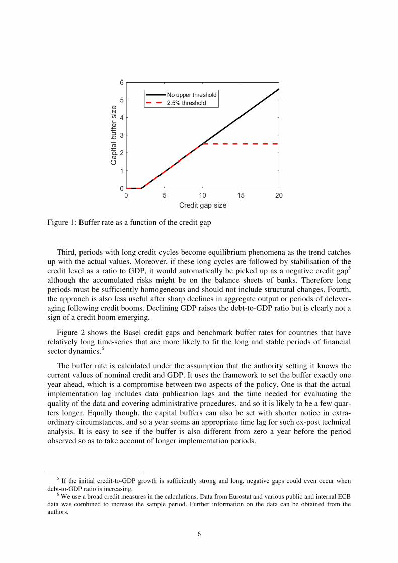
The Basel framework also explains how the capital buffer could be set using the credit gap. Figure 1 shows the buffer size graphically as a function of the gap size. The buffer is zero when the credit gap is smaller than 2 percentage points and it increases linearly to reach 2.5% of the capital3 when the credit gap hits 10 pp. The suggested buffer size increases by 0.3125% with each additional credit gap percentage point. The buffer size for the banks is then rounded to the buffer step size of 0.25%.

There are two possible versions of the buffer settings that have not been fully tested in practice. In the first version the buffer rate is increased linearly as the credit gap increases (the solid black line in Figure 1), and in the second version there is an upper limit of 2.5% for the buffer rate (the dashed red line). In this scenario, either the national authority does not in-crease capital buffers above that value or other countries do not have to recognise levels that exceed that threshold (in the EU a ‘comply or explain’ procedure would then follow according to the ESRB Recommendation4).

The main weakness of the Basel framework for calculating credit gaps is that it requires long data-series to pick up the trends values for financial deepening from the early periods. Only after the initial years have set the trend can a change in the debt-to-GDP ratio signal a possible credit cycle.

A second weakness is that the approach requires long data-series for it to be able to estimate the trend value, but the early data that are used in the calculations might have be-come uninformative about the current state of the economy. For example, Estonia started with a very low level of financial depth that is not likely to return in the near future.

3 The buffer size is calculated as a percentage of the capital, for space flow reasons the buffers are referred to

as per cents without reference to the capital. 4 Recommendation of the European Systemic Risk Board of 18 June 2014 on guidance for setting counter-

cyclical buffer rates (ESRB/2014/1).

6

Figure 1: Buffer rate as a function of the credit gap

Third, periods with long credit cycles become equilibrium phenomena as the trend catches up with the actual values. Moreover, if these long cycles are followed by stabilisation of the credit level as a ratio to GDP, it would automatically be picked up as a negative credit gap5 although the accumulated risks might be on the balance sheets of banks. Therefore long periods must be sufficiently homogeneous and should not include structural changes. Fourth, the approach is also less useful after sharp declines in aggregate output or periods of delever-aging following credit booms. Declining GDP raises the debt-to-GDP ratio but is clearly not a sign of a credit boom emerging.

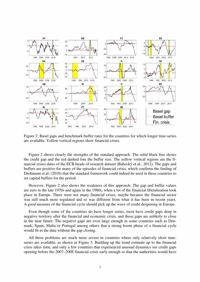
Figure 2 shows the Basel credit gaps and benchmark buffer rates for countries that have relatively long time-series that are more likely to fit the long and stable periods of financial sector dynamics.6

The buffer rate is calculated under the assumption that the authority setting it knows the current values of nominal credit and GDP. It uses the framework to set the buffer exactly one year ahead, which is a compromise between two aspects of the policy. One is that the actual implementation lag includes data publication lags and the time needed for evaluating the quality of the data and covering administrative procedures, and so it is likely to be a few quar-ters longer. Equally though, the capital buffers can also be set with shorter notice in extra-ordinary circumstances, and so a year seems an appropriate time lag for such ex-post technical analysis. It is easy to see if the buffer is also different from zero a year before the period observed so as to take account of longer implementation periods.

5 If the initial credit-to-GDP growth is sufficiently strong and long, negative gaps could even occur when

debt-to-GDP ratio is increasing. 6 We use a broad credit measures in the calculations. Data from Eurostat and various public and internal ECB

data was combined to increase the sample period. Further information on the data can be obtained from the authors.

7

Figure 2: Basel gaps and benchmark buffer rates for the countries for which longer time-series are available. Yellow vertical regions show financial crises.

Figure 2 shows clearly the strengths of the standard approach. The solid black line shows the credit gap and the red dashed line the buffer size. The yellow vertical regions are the fi-nancial crises dates of the ECB heads of research dataset (Babecký et al., 2012). The gaps and buffers are positive for many of the episodes of financial crisis, which confirms the finding of Drehmann et al. (2010) that the standard framework could indeed be used in these countries to set capital buffers for the period.

However, Figure 2 also shows the weakness of this approach. The gap and buffer values are zero in the late 1970s and again in the 1980s, when a lot of the financial liberalisation took place in Europe. There were not many financial crises, maybe because the financial sector was still much more regulated and so was different from what it has been in recent years. A good measure of the financial cycle should pick up the wave of credit deepening in Europe.

Even though some of the countries do have longer series, most have credit gaps deep in negative territory after the financial and economic crisis, and those gaps are unlikely to close in the near future. The negative gaps are even large enough in some countries such as Den-mark, Spain, Malta or Portugal among others that a strong boom phase of a financial cycle would fit in the data without the gap closing.

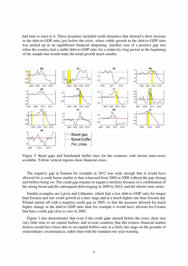
All these problems are much more severe in countries where only relatively short time-series are available, as shown in Figure 3. Building up the trend estimate up to the financial crisis takes time, and only a few countries that experienced unusual dynamics see credit gaps opening before the 2007–2008 financial crisis early enough so that the authorities would have

8

had time to react to it. These dynamics included credit dynamics that showed a short increase in the debt-to-GDP ratio just before the crisis, where stable growth in the debt-to-GDP ratio was picked up as an equilibrium financial deepening. Another case of a positive gap was when the country had a stable debt-to-GDP ratio for a relatively long period at the beginning of the sample that would make the trend growth much smaller.

Figure 3: Basel gaps and benchmark buffer rates for the countries with shorter time-series available. Yellow vertical regions show financial crises.

The negative gap in Estonia for example in 2012 was wide enough that it would have allowed for a credit boom similar to that witnessed from 2004 to 2008 without the gap closing and buffers being set. The credit gap remains in negative territory because of a combination of the strong boom and the subsequent deleveraging in 2009 to 2014, and the shorter time series.

Similar examples are Latvia and Lithuania, which had a low debt-to GDP ratio for longer than Estonia and saw credit growth at a later stage and at a much higher rate than Estonia did. Poland started off with a negative credit gap in 2005, so that the measure allowed for much higher change in the debt-to GDP ratio than for example it would have allowed for Croatia that had a credit gap close to zero in 2005.

Figure 3 also demonstrates that even if the credit gaps opened before the crisis, there was very little time to set capital buffers, and several countries that did witness financial market distress would have been able to set capital buffers only at a fairly late stage on the grounds of extraordinary circumstances, rather than with the standard one-year warning.

9

3. New gaps The paper suggests four additional measures for the gap alongside the standard Basel frame-work. (1) Change in the debt-to-GDP ratio, over a two-year period (2 y change). (2) Nominal debt growth minus average nominal GDP growth over eight years, over a two-

year period (8 y average). (3) Nominal debt growth minus 5% annually, over a two-year period (5% rule). (4) Change in the ratio of nominal debt to the nominal GDP trend, over a two-year period,

where trend GDP is an exponent of the one-sided HP filtered (with the smoothing pa-rameter ) = 400000) log of nominal trend GDP (GDP trend).

These measures are selected because they have simple rules that do not require expert judgement in the calculations, and so they can all be used directly by anyone who has the underlying data. They should also be free of the main weaknesses of the HP filter, as they do not require long time-series to extract the cycles, they do not depend on credit developments as long as 15 years ago, and they pick up long cycles and are informative at times when GDP is decreasing and in periods of deleveraging.

This allows the future situation to be analysed using current knowledge, and the result is less sensitive to the potential psychological biases that come from accepting the current situation as equilibrium dynamics. Using different measures also recognises explicitly that no single measure can be perfect, so different measures pick up possible scenarios in different economic environments. (1) Change in the debt-to-GDP ratio

The change in the debt-to-GDP ratio over two years picks up the type of credit cycle where credit growth is stronger than nominal GDP growth within the two-year period. The exact formula is:

����+,-�./! = 100 ∗ 1 ����˗�'˗��������˗�'˗�����2 − 13. The main strength of this is that it does not depend on a long history. With this approach

every change in the debt-to-GDP ratio that lasts for two years opens a gap that could be a sign of a financial cycle.

The main weakness is that it can miss a credit boom that is accompanied by a nominal GDP boom that may or may not be caused by credit developments. It would also show positive credit gaps when nominal GDP falls faster than credit aggregate, though this should not be interpreted directly as a credit boom.

(2) Nominal debt growth relative to average GDP growth

The second approach compares the nominal credit growth over two years with the average GDP growth rate over eight years. The number of years is selected to cover a sufficiently long window so that business cycle developments can be picked up without data that might have become irrelevant being included. The exact formula for the calculations is:

10

���2+56.7%5 = 100 ∗ 1 ���������2 − 13 − 100 ∗ ����89':�ℎ , where the average growth of the eight years is taken to the power of eight to get the accumulated change in GDP over an eight-quarter period:

����89':�ℎ = <1 + 1100 132?100 ∗ 1 ���������� − 13��

6@AB2.

The main strength of the approach is that it does not depend on long time series. Another is that it recognises shorter credit booms that the change in the debt-to-GDP ratio cannot pick up as it uses averages over longer periods. It also is free of the problem of sudden drops in GDP increasing the gap.

The main weakness is that it does not pick up booms when they are long and possibly driven by credit growth. This might happen because average nominal growth becomes similar to nominal credit growth and the gaps remain close to zero.

(3) Nominal debt growth relative to 5% nominal growth

This approach uses a fixed denominator of 5% annually. The 5% rule could be interpreted as real GDP growth of 2% and GDP deflator inflation of 2% annually with an extra margin of 1% to compensate for possible Estonian economic and price level convergence with the EU average during the coming years. The exact formula is:

���C%EF"! = 100 ∗ 1 ���������2 − 13 − 100 ∗ &1.05� − 1(. Unlike the measure that uses the eight-year period, it is not sensitive to credit driven booms

that result in either high real GDP growth or strong GDP inflation rates. It is also easy to cal-culate and intuitive to understand. Ideally the growth rate of the underlying unobservable potential nominal GDP could be used instead. However real time estimates of potential real GDP are not very reliable and tend to be biased towards realised growth rates, and there is no standard methodology for calculating the growth rate of the equilibrium GDP deflator.

The problem is that the 5% rule of thumb does not fit for all periods, such as those when there is low equilibrium nominal growth, and historically many countries have had high levels of growth or periods of high inflation that were followed by exchange rate adjustments. (4) Nominal debt relative to trend GDP

This final measure compares the level of debt to a trend value for GDP. The measure is close to the first alternative of the change in the debt-to-GDP ratio over a two-year period, but the ratio is calculated relative to the GDP trend value. The equation used in the calculations is:

���HIJE!.7 = 100 × K����˗�'˗����E����˗�'˗�����2E − 1L,

11

where the level values of GDP are used to calculate trend GDP:

����E = exp&$�% &O�&����(((, where in turn the trend GDP is summed over the previous four quarters as in the original Basel framework7.

The main strength of this compared to Basel framework is that it opens positive gaps when credit booms are accompanied by GDP booms. The trend estimation should take growth potential into account over longer periods. Equally, it does not open negative gaps during periods of negative nominal GDP growth.

The main weakness is that it requires a good estimate of the trend GDP, and the approach suggested is only one way to calculate the trend value. It is also more complicated and less intuitive to understand.

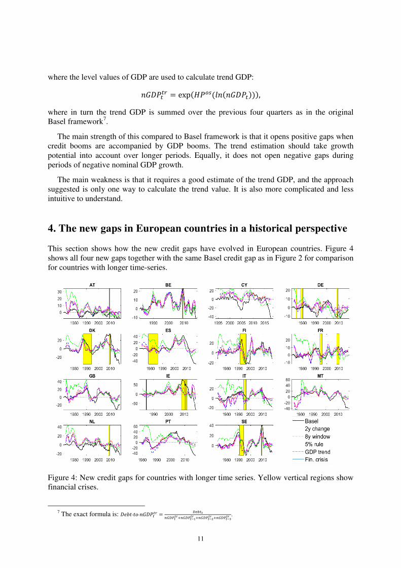
4. The new gaps in European countries in a historical perspective This section shows how the new credit gaps have evolved in European countries. Figure 4 shows all four new gaps together with the same Basel credit gap as in Figure 2 for comparison for countries with longer time-series.

Figure 4: New credit gaps for countries with longer time series. Yellow vertical regions show financial crises.

7 The exact formula is: ����˗�'˗����E = I!PQ.HIJQQRS.HIJQTUQR S.HIJQTVQR S.HIJQTWQR .

12

For most of the periods, all the calculated gaps behave quite similarly. Credit cycles in Belgium for example look similar in frequency and size for all the measures. There are however several noticeable differences between the standard Basel gap and the new gaps suggested here.

First, the new gaps do not show substantial negative gaps for the years after the financial crisis, as some are still slightly negative but some are in positive territory. This shows that the new gaps do not depend on long time-series like the Basel benchmark does. Second, the early periods of the sample in the 1970s and 1980s do not have zero gaps in many countries, including Austria, Cyprus and Germany.

As expected the 5% rule behaves very differently in the countries that witnessed strong nominal GDP growth rates in the 1970s and 1980s. It opens positive gaps that are much larger than those from other measures. This means that in these countries banks and other institu-tions giving credit provided larger and larger numbers of loans at that time. Europe did not face many financial crises during that period, but general economic conditions, the perfor-mance of the financial sector, and regulations governing the financial sector were different from what they were in the 2000s. It is likely that such a rule of thumb for monitoring cycles would not have been put in place at that time as the particular value is set for looking to the future, but it gives a picture of how the rules would have evolved

The overall conclusion is that the variability of the new measures is fairly similar to that for the Basel credit gap in the middle of the sample, which is the period where the Basel gap measures cycles well. This is taken as a sign of the strength of the new gap measures. Differences in the early and late periods are also to be expected and taken as a positive sign rather than a negative one.

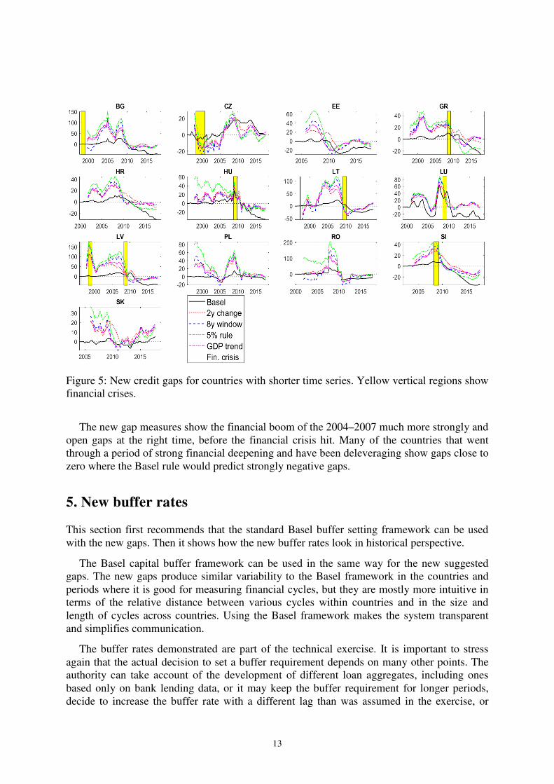
Figure 5 shows that the variability of the new measures for countries with shorter samples is often very different from that for the Basel measures. This happens because in broad terms the sample consists of two periods, an early period when the Basel gap is close to zero because of the initialisation of the trend, and the post 2008 crisis period where the Basel framework has become less informative.

13

Figure 5: New credit gaps for countries with shorter time series. Yellow vertical regions show financial crises.

The new gap measures show the financial boom of the 2004–2007 much more strongly and open gaps at the right time, before the financial crisis hit. Many of the countries that went through a period of strong financial deepening and have been deleveraging show gaps close to zero where the Basel rule would predict strongly negative gaps.

5. New buffer rates This section first recommends that the standard Basel buffer setting framework can be used with the new gaps. Then it shows how the new buffer rates look in historical perspective.

The Basel capital buffer framework can be used in the same way for the new suggested gaps. The new gaps produce similar variability to the Basel framework in the countries and periods where it is good for measuring financial cycles, but they are mostly more intuitive in terms of the relative distance between various cycles within countries and in the size and length of cycles across countries. Using the Basel framework makes the system transparent and simplifies communication.

The buffer rates demonstrated are part of the technical exercise. It is important to stress again that the actual decision to set a buffer requirement depends on many other points. The authority can take account of the development of different loan aggregates, including ones based only on bank lending data, or it may keep the buffer requirement for longer periods, decide to increase the buffer rate with a different lag than was assumed in the exercise, or

14

release the buffer requirement before the gaps close. However, as the objective of the current exercise is to look at how the credit gaps would suggest buffer sizes and to evaluate their use-fulness in the historical perspective, it is instructive to look at the predicted buffer rates.

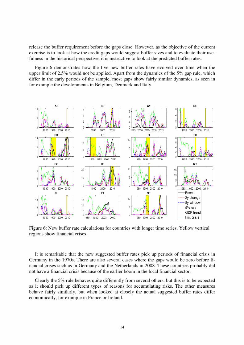
Figure 6 demonstrates how the five new buffer rates have evolved over time when the upper limit of 2.5% would not be applied. Apart from the dynamics of the 5% gap rule, which differ in the early periods of the sample, most gaps show fairly similar dynamics, as seen in for example the developments in Belgium, Denmark and Italy.

Figure 6: New buffer rate calculations for countries with longer time series. Yellow vertical regions show financial crises.

It is remarkable that the new suggested buffer rates pick up periods of financial crisis in Germany in the 1970s. There are also several cases where the gaps would be zero before fi-nancial crises such as in Germany and the Netherlands in 2008. These countries probably did not have a financial crisis because of the earlier boom in the local financial sector.

Clearly the 5% rule behaves quite differently from several others, but this is to be expected as it should pick up different types of reasons for accumulating risks. The other measures behave fairly similarly, but when looked at closely the actual suggested buffer rates differ economically, for example in France or Ireland.

15

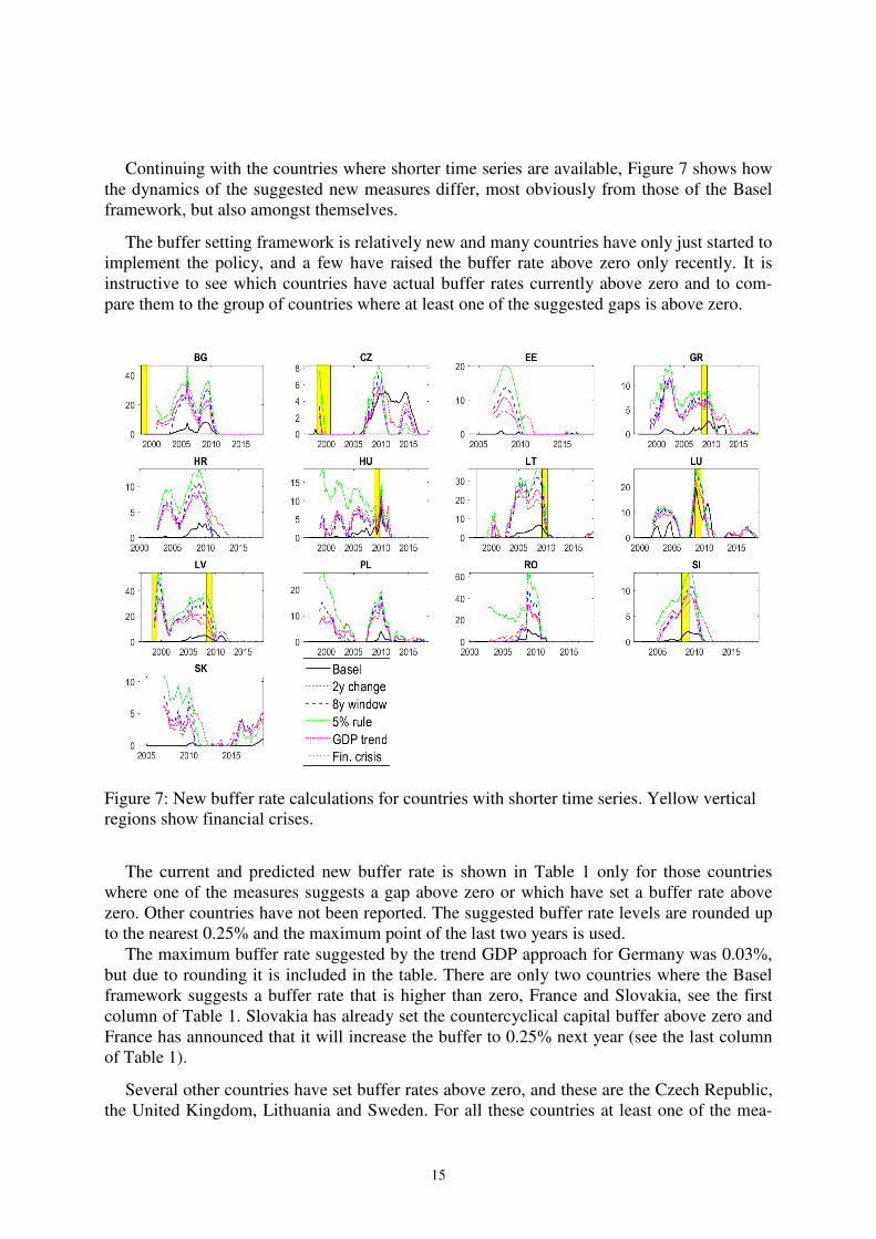
Continuing with the countries where shorter time series are available, Figure 7 shows how the dynamics of the suggested new measures differ, most obviously from those of the Basel framework, but also amongst themselves.

The buffer setting framework is relatively new and many countries have only just started to implement the policy, and a few have raised the buffer rate above zero only recently. It is instructive to see which countries have actual buffer rates currently above zero and to com-pare them to the group of countries where at least one of the suggested gaps is above zero.

Figure 7: New buffer rate calculations for countries with shorter time series. Yellow vertical regions show financial crises.

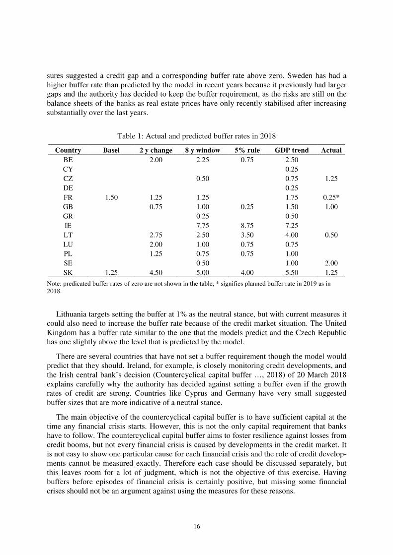
The current and predicted new buffer rate is shown in Table 1 only for those countries where one of the measures suggests a gap above zero or which have set a buffer rate above zero. Other countries have not been reported. The suggested buffer rate levels are rounded up to the nearest 0.25% and the maximum point of the last two years is used.

The maximum buffer rate suggested by the trend GDP approach for Germany was 0.03%, but due to rounding it is included in the table. There are only two countries where the Basel framework suggests a buffer rate that is higher than zero, France and Slovakia, see the first column of Table 1. Slovakia has already set the countercyclical capital buffer above zero and France has announced that it will increase the buffer to 0.25% next year (see the last column of Table 1).

Several other countries have set buffer rates above zero, and these are the Czech Republic, the United Kingdom, Lithuania and Sweden. For all these countries at least one of the mea-

16

sures suggested a credit gap and a corresponding buffer rate above zero. Sweden has had a higher buffer rate than predicted by the model in recent years because it previously had larger gaps and the authority has decided to keep the buffer requirement, as the risks are still on the balance sheets of the banks as real estate prices have only recently stabilised after increasing substantially over the last years.

Table 1: Actual and predicted buffer rates in 2018

Country Basel 2 y change 8 y window 5% rule GDP trend Actual

BE 2.00 2.25 0.75 2.50 CY 0.25 CZ 0.50 0.75 1.25 DE 0.25 FR 1.50 1.25 1.25 1.75 0.25* GB 0.75 1.00 0.25 1.50 1.00 GR 0.25 0.50 IE 7.75 8.75 7.25 LT 2.75 2.50 3.50 4.00 0.50 LU 2.00 1.00 0.75 0.75 PL 1.25 0.75 0.75 1.00 SE 0.50 1.00 2.00 SK 1.25 4.50 5.00 4.00 5.50 1.25

Note: predicated buffer rates of zero are not shown in the table, * signifies planned buffer rate in 2019 as in 2018.

Lithuania targets setting the buffer at 1% as the neutral stance, but with current measures it could also need to increase the buffer rate because of the credit market situation. The United Kingdom has a buffer rate similar to the one that the models predict and the Czech Republic has one slightly above the level that is predicted by the model.

There are several countries that have not set a buffer requirement though the model would predict that they should. Ireland, for example, is closely monitoring credit developments, and the Irish central bank’s decision (Countercyclical capital buffer …, 2018) of 20 March 2018 explains carefully why the authority has decided against setting a buffer even if the growth rates of credit are strong. Countries like Cyprus and Germany have very small suggested buffer sizes that are more indicative of a neutral stance.

The main objective of the countercyclical capital buffer is to have sufficient capital at the time any financial crisis starts. However, this is not the only capital requirement that banks have to follow. The countercyclical capital buffer aims to foster resilience against losses from credit booms, but not every financial crisis is caused by developments in the credit market. It is not easy to show one particular cause for each financial crisis and the role of credit develop-ments cannot be measured exactly. Therefore each case should be discussed separately, but this leaves room for a lot of judgment, which is not the objective of this exercise. Having buffers before episodes of financial crisis is certainly positive, but missing some financial crises should not be an argument against using the measures for these reasons.

17

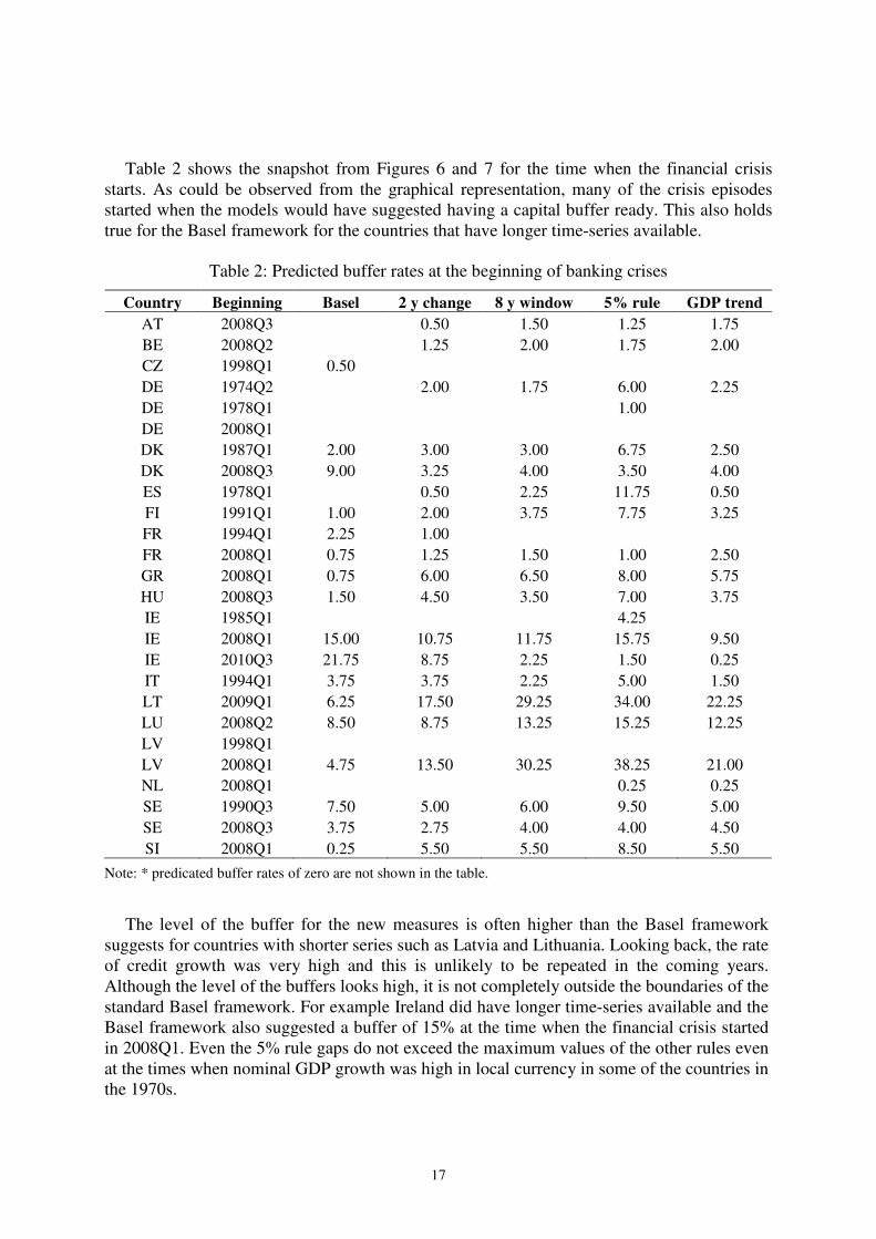
Table 2 shows the snapshot from Figures 6 and 7 for the time when the financial crisis starts. As could be observed from the graphical representation, many of the crisis episodes started when the models would have suggested having a capital buffer ready. This also holds true for the Basel framework for the countries that have longer time-series available.

Table 2: Predicted buffer rates at the beginning of banking crises

Country Beginning Basel 2 y change 8 y window 5% rule GDP trend

AT 2008Q3 0.50 1.50 1.25 1.75 BE 2008Q2 1.25 2.00 1.75 2.00 CZ 1998Q1 0.50 DE 1974Q2 2.00 1.75 6.00 2.25 DE 1978Q1 1.00 DE 2008Q1 DK 1987Q1 2.00 3.00 3.00 6.75 2.50 DK 2008Q3 9.00 3.25 4.00 3.50 4.00 ES 1978Q1 0.50 2.25 11.75 0.50 FI 1991Q1 1.00 2.00 3.75 7.75 3.25 FR 1994Q1 2.25 1.00 FR 2008Q1 0.75 1.25 1.50 1.00 2.50 GR 2008Q1 0.75 6.00 6.50 8.00 5.75 HU 2008Q3 1.50 4.50 3.50 7.00 3.75 IE 1985Q1 4.25 IE 2008Q1 15.00 10.75 11.75 15.75 9.50 IE 2010Q3 21.75 8.75 2.25 1.50 0.25 IT 1994Q1 3.75 3.75 2.25 5.00 1.50 LT 2009Q1 6.25 17.50 29.25 34.00 22.25 LU 2008Q2 8.50 8.75 13.25 15.25 12.25 LV 1998Q1 LV 2008Q1 4.75 13.50 30.25 38.25 21.00 NL 2008Q1 0.25 0.25 SE 1990Q3 7.50 5.00 6.00 9.50 5.00 SE 2008Q3 3.75 2.75 4.00 4.00 4.50 SI 2008Q1 0.25 5.50 5.50 8.50 5.50

Note: * predicated buffer rates of zero are not shown in the table.

The level of the buffer for the new measures is often higher than the Basel framework suggests for countries with shorter series such as Latvia and Lithuania. Looking back, the rate of credit growth was very high and this is unlikely to be repeated in the coming years. Although the level of the buffers looks high, it is not completely outside the boundaries of the standard Basel framework. For example Ireland did have longer time-series available and the Basel framework also suggested a buffer of 15% at the time when the financial crisis started in 2008Q1. Even the 5% rule gaps do not exceed the maximum values of the other rules even at the times when nominal GDP growth was high in local currency in some of the countries in the 1970s.

18

6. Summary The Basel framework for calculating credit gaps and corresponding rates for the counter-cyclical capital buffer suffers from several weaknesses that have materialised since the finan-cial crisis of 2007 and the great recession that followed. This paper suggests alternative ways of measuring credit gaps and suggests a way to set capital buffers that is free from the main weaknesses of the original rule but retains the wanted property that the benchmark buffer rates are sizable at the time when a financial crisis hits.

19

References

BABECKÝ, J.; HAVRANEK, T.; MATEJU, J.; RUSNÁK, M.; SMIDKOVA, K.; VASICEK, B. (2012): Banking, Debt and Currency Crises: Early Warning Indicators for Developed Countries. ECB Working Paper, No 1485.

BASEL III: A global regulatory framework for more resilient banks and banking systems (2011). Bank of International Settlements, December 2010 (rev June 2011).

COUNTERCYCLICAL CAPITAL BUFFER RATE ANNOUNCEMENT (2018). Central Bank of Ireland, March 20th 2018, https://www.centralbank.ie/docs/default-source/financial-system/financial-stability/macroprudential-policy/countercyclical-capital-buffer/ccyb-rate-announcement-march-2018.pdf?sfvrsn=4

DREHMANN, M.; BORIO, C.; GAMBACORTA, L.; JIMÉNEZ, G.; TRUCHARTE, C. (2010): Countercyclical capital buffers: exploring options. Bank of International Settlements Working Papers, No 317.

DREHMANN, M.; TSATSARONIS, K. (2014): The credit-to-GDP gap and countercyclical capital buffers: questions and answers. Bank of International Settlements Quarterly

Review, March 2014.

DREHMANN, M.; YETMAN, J. (2018): Why you should use the Hodrick-Prescott filter - at least to generate credit gaps. Bank of International Settlements Working Papers, No 744.

EDGE, R.M.; MEISENZAHL, R.R. (2011): The Unreliability of Credit-to-GDP Ratio Gaps in Real Time: Implications for Countercyclical Capital Buffers. International Journal of

Central Banking, 7(4), pp. 261–298.

Working Papers of Eesti Pank 2018

No 1Sang-Wook (Stanley), Cho Julián P. Daz. Skill premium divergence: the roles of trade, capital and demographics

No 2Wenjuan Chen, Aleksei Netšunajev. Structural vector autoregression with time varying transition probabilities: identifying uncertainty shocks via changes in volatility

No 3Eva Branten, Ana Lamo, Tairi Rõõm. Nominal wage rigidity in the EU countries before andafter the Great Recession: evidence from the WDN surveys

No 4Merike Kukk, Alari Paulus, Karsten Staehr. Income underreporting by the self-employed in Europe: A cross-country comparative study

No 5Juan Carlos Cuestas, Estefania Mourelle, Paulo José Regis. Real exchange rate misalignments in CEECs: Have they hindered growth?

No 6Juan Carlos Cuestas. Changes in sovereign debt dynamics in Central and Eastern Europe