WP-2014-032

Why Tax Effort Falls Short of Capacity in Indian States: A StochasticFrontier Approach*

Sandhya Garg, Ashima Goyal**, Rupayan Pal**

Indira Gandhi Institute of Development Research, MumbaiAugust 2014

http://www.igidr.ac.in/pdf/publication/WP-2014-032.pdf

Why Tax Effort Falls Short of Capacity in Indian States: A StochasticFrontier Approach*

Sandhya Garg, Ashima Goyal**, Rupayan Pal**Indira Gandhi Institute of Development Research (IGIDR)

General Arun Kumar Vaidya Marg Goregaon (E), Mumbai- 400065, INDIA

Email(corresponding author): ashima@igidr.ac.in

AbstractTaxation is an important tool to enhance the economic development and to finance the expenditure

responsibilities of a government. This paper attempts to measure the tax capacity and tax effort of 14

major Indian states from 1992-92 to 2010-11 using Stochastic Frontier Analysis. The use of tax capacity

frontier helps to identify those states which are operating near their tax capacity and states which are

away from tax frontier. The results indicate presence of large variation in tax effort index across states

and which seems to be increasing over time. Econometric analysis suggests that economic and

structural variables have significant impact on the tax capacity. While per-capita gross state domestic

product has positive effect on states' own tax revenue, relative size of agriculture sector of a state has

adverse effect on its own tax revenue. The evidence on tax efficiency suggests that the higher

inter-governmental transfers tend to reduce tax efficiency. Outstanding liabilities and expenditure on

debt repayment also indicate adverse effect on tax efficiency, but the adverse effect of the latter is lesser

than the former. Enactment of Fiscal Responsibility and Budget Management Act seems to have

improved the tax efficiency which has been further strengthened by the better law and order inside

states. Higher political competition inside a state, represented by effective number of parties, has

favourable effect on the tax efficiency of a state. Implications are drawn for policy.

Keywords: tax capacity, tax effort, stochastic frontier analysis, fiscal federalism

JEL Code: H21, H29, H71, H77

Acknowledgements:

*This paper is based on the first author's Ph. D. work.

** Authors are faculty at Indira Gandhi Institute of Development Research.

Why Tax Effort Falls Short of Capacity in Indian States: A

Stochastic Frontier Approach*

Table of Content

1. Introduction ..................................................................................................................................... 1

2. Federal Structure in Indian Economy ............................................................................................. 3

2.1 Major Taxes .............................................................................................................................. 3

2.2 Federal Transfers....................................................................................................................... 5

2.3 Debt ........................................................................................................................................... 8

3. Methodological Developments ....................................................................................................... 8

3.1. Income Approach .................................................................................................................. 8

3.2. Representative Tax System ................................................................................................... 9

3.3. Aggregate Regression Approach.............................................................................................. 9

3.4. Stochastic Frontier Approach (SFA) ...................................................................................... 10

4. Data and Variables ........................................................................................................................ 13

4.1. Dependent Variable................................................................................................................ 13

4.2. Explanatory Variables for Estimating Tax Capacity ............................................................. 14

4.3. Explanatory Variables for Inefficiency Equation .................................................................. 15

4.4. Political Variables .................................................................................................................. 18

5. Political Economy of Inter-governmental Transfers ................................................................. 20

6. Computation of Tax Capacity and Tax Effort: Individual States.............................................. 23

6.1. Interpreting the Inefficiency Equation .................................................................................. 24

6.2. Tax Effort Index .................................................................................................................... 26

7. Conclusion ................................................................................................................................ 29

References ......................................................................................................................................... 32

Appendices ........................................................................................................................................ 36

ii

List of Tables

Table 1:Various Sources of Revenue: All States (1991-91 to 2010-11) ................................... 4

Table 2: Dependence of Individual States on Fiscal Transfers from Centre ............................. 7

Table 3: Summary Statistics .................................................................................................... 20

Table 4: Relation between Inter-governmental Transfers and the Political Environment

(1991-2010): Fixed Effect Panel Data Model .......................................................................... 22

Table 5: Simultaneous Estimation of Tax Revenue and Technical Inefficiency: Stochastic

Frontier Approach (1992-93 to 2010-11) ................................................................................ 25

Table 6: Tax Effort Index and Rank of States: SFA Approach (1992, 2001, 2010) ............... 27

Table 7: Sigma convergence in Tax Efficiency Score ............................................................. 28

iii

List of Figures

Figure 1: Variation in Own Tax Revenue relative to GSDP: All States (1991-92 to 2010-11) 5

Figure 2: Trend in the Efficiency Score of States (1992-2010) ............................................... 27

1

1. Introduction

India with 29 states and 6 union territories possesses a federal structure which specifies three

characteristics for different tiers of governments: division of functional responsibilities,

assignment of autonomous revenue sources and system of inter-governmental fiscal transfers

(Bagchi, 2003). Exclusive powers of central and state governments are specified in Union list

and State list respectively. The subjects like defence, macroeconomic stability, money and

banking, international trade etc. are assigned to the central government in union list. The

functions entrusted to the state governments are those of maintaining public order, agriculture

sector, public health and sanitation, water supply, and irrigation etc. The powers falling in

common jurisdiction are specified under concurrent list and these include education,

transportation and social insurance etc. (Rao and Singh, 2007; Bagchi, 2003). Similar to the

expenditure function of the governments, the revenue sources are also divided. Central

government is assigned with taxes which have broad and mobile bases like tax on income and

wealth from non-agriculture sources, corporation tax, custom duties etc. Taxes within

jurisdiction of state governments include tax on income and wealth from agriculture sector,

sales tax, certain excise duties etc. Apart from the taxation power of states, constitution made

recommendations for additional revenue sources to states as well, which includes sharing the

proceeds of centrally levied taxes and providing grants from Consolidated Fund of India.

These transfers help states to bridge the gap between expenditure and their own revenue. The

idea behind these transfers is to achieve uniformity in public services and the tax rates all

over the country along with avoiding tax evasion and the high cost of decentralized

collection.

The distribution of tax assignments between centre and states ensures fiscal autonomy to

states up to some extent and makes for an effective federal structure. It is based on the

principle of separation which indicates that the tax assignments between centre and state

governments are mutually exclusive (Rao and Singh, 2007).Taxation, among all revenue

sources1 is an important tool to finance the expenditure responsibilities for state governments.

Large differences in the expenditure pattern at the sub-national level (Rao et. al.,1999;

Bagchi, 2003) calls for a study of the revenue sources of states. Concepts related to revenue

sources of the government are revenue capacity and tax capacity. Revenue capacity/potential

1 Other revenue sources of states are: Inter-governmental transfers such as share in central taxes, grants, and

loans from the central government; loans from the market; interest receipts; dividends etc.

2

is a broader term which includes total tax and non-tax revenue capacity of different fiscal

entities. It refers to the maximum revenue a government can generate given its economic,

social, administrative, demographic and other characteristics.

The object of this study is to analyse the revenue sources of the state governments in general,

and their own tax collection in particular. As states impose certain kind of taxes and retain

that revenue hence it is important to study their own tax capacity/potential2along with actual

tax collection. Stochastic Frontier Analysis (SFA) is used to estimate own tax capacity at the

sub-national level for the period of 1992-93 to 2010-11, which is further used to compute tax

effort. Tax capacity similar to revenue capacity, refers to the maximum potential tax revenue

a government can generate. Tax effort on the other hand is the comparison of actual tax

collection and tax capacity. This in simple terms can be defined as the ability to raise tax

revenue which can further be realized by imposing different kinds of tax policies. More

specifically we investigate the determinants of own tax revenue of state governments.

Alfirman (2003) suggest that unlike output frontier where specific inputs i.e. capital and

labour determine the output, the tax frontier is not subjected to specific inputs. As underlying

relationship of tax revenue and its input factors is not very clear, implication of several

factors has been analysed on tax capacity. Guided by the literature, a comprehensive data set

has been used which covers economic, social, demographic, governance, and political aspects

of states. These variables will help to identify factors to increase tax collection of less

performing states.

There are few Indian studies on the determinants of tax collection. The use of better panel

data methodology while incorporating several aspects of state economies is missing so far in

estimation of tax capacity. This study fills this gap by providing improved estimates of tax

capacity and tax effort using SFA. Construction of tax frontier at sub-national level will

enable us to identify states performing near tax frontier i.e. collecting taxes near their tax

capacity, and states which are far below their tax capacity. Based on these estimates all states

are ranked from low tax effort to high tax effort. Low tax effort signifies that a state has not

utilized its tax capacity fully relative to other states and vice-versa.

We aim to answer the following questions:

(i) What is the role of economic structure on the tax capacity?

2The terms Tax Capacity and Tax Potential have been used interchangeably.

3

(ii) What is the relative tax effort index of states?

(iii) Do federal transfers have any adverse effect on tax effort?

(iv) How has Fiscal Responsibility and Budget Management Act (FRBMA) affected

tax effort?

(v) How does the political environment of a state affect its tax effort?

Our results indicate that economic and structural variables significantly affect the tax capacity

of states. While per-capita Gross State Domestic Product (GSDP) has positive and significant

association with tax collection of states, the agriculture sector with lesser contribution in

aggregate tax revenue (Table, 1) reduces tax collection. Federal transfers adversely affect

states’ tax efficiency. Total outstanding liabilities and debt repayment of states also put

adverse effect on the tax efficiency whereas the effect of the latter is lesser than the former.

On the other hand, larger expenditure responsibility and better governance index of a state

have favourable effect on the tax efficiency which has further improved with enactment of

FRBMA. As far as political variables are concerned, the results show that effective number of

parties which indicates the political competition inside a state has favourable effect on its tax

efficiency.

The structure of this paper is organised as follows. Section 2 presents the brief overview of

various revenue sources of the states such as: their own tax revenue, federal transfers, debt

and FRBMA. Section 3 documents the literature review and methodological developments,

where the methodology of SFA is explained. Section 4 gives the detail of all the variables. In

section 5 the political economy of federal transfers is studied. Section 6 represents the

computation of tax capacity and tax effort. Section 7 presents the concluding remarks.

2. Federal Structure in Indian Economy

In this section we give brief introduction about important features of Indian federal structure.

First, we give brief overview of share of each tax in total tax revenue, which is followed by

contribution of federal transfers and debt. Also brief description of enactment of FRBMA is

given.

2.1 Major Taxes

Table (1) presents total revenue and the relative share of its various components in total

revenue. These components consist of states’ own tax revenue; transfers from central

government and various ministries; borrowing; and other revenue sources. Own tax revenue

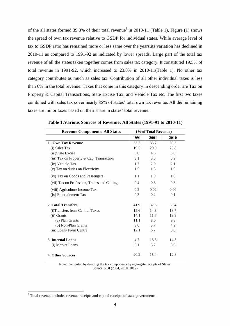
4

of the all states formed 39.3% of their total revenue3 in 2010-11 (Table 1). Figure (1) shows

the spread of own tax revenue relative to GSDP for individual states. While average level of

tax to GSDP ratio has remained more or less same over the years,its variation has declined in

2010-11 as compared to 1991-92 as indicated by lower spreads. Large part of the total tax

revenue of all the states taken together comes from sales tax category. It constituted 19.5% of

total revenue in 1991-92, which increased to 23.8% in 2010-11(Table 1). No other tax

category contributes as much as sales tax. Contribution of all other individual taxes is less

than 6% in the total revenue. Taxes that come in this category in descending order are Tax on

Property & Capital Transactions, State Excise Tax, and Vehicle Tax etc. The first two taxes

combined with sales tax cover nearly 85% of states’ total own tax revenue. All the remaining

taxes are minor taxes based on their share in states’ total revenue.

Table 1:Various Sources of Revenue: All States (1991-91 to 2010-11)

Revenue Components: All States (% of Total Revenue)

1991 2001 2010

1. Own Tax Revenue 33.2 33.7 39.3

(i) Sales Tax 19.5 20.0 23.8

(ii )State Excise 5.0 4.5 5.0

(iii) Tax on Property & Cap. Transaction 3.1 3.5 5.2

(iv) Vehicle Tax 1.7 2.0 2.1

(v) Tax on duties on Electricity 1.5 1.3 1.5

(vi) Tax on Goods and Passengers 1.1 1.0 1.0

(vii) Tax on Profession, Trades and Callings 0.4 0.8 0.3

(viii) Agriculture Income Tax 0.2 0.02 0.00

(ix) Entertainment Tax 0.3 0.2 0.1

2. Total Transfers 41.9 32.6 33.4

(i)Transfers from Central Taxes 15.6 14.3 18.7

(ii) Grants 14.1 11.7 13.9

(a) Plan Grants 11.1 8.0 9.8

(b) Non-Plan Grants 3.0 3.7 4.2

(iii) Loans From Centre 12.1 6.7 0.8

3. Internal Loans 4.7 18.3 14.5

(i) Market Loans 3.1 5.2 8.9

4. Other Sources 20.2 15.4 12.8

Note: Computed by dividing the tax components by aggregate receipts of States.

Source: RBI (2004, 2010, 2012)

3 Total revenue includes revenue receipts and capital receipts of state governments.

5

Figure 1: Variation in Own Tax Revenue Relative to GSDP: All States (1991-92 to 2010-

11)

Computed by dividing the Own tax revenue by GSDP (at current prices).

Source: RBI (2004, 2010, 2012)

2.2 Federal Transfers

Federal transfers are shared with States through many channels, i.e. (a) Finance Commission

(FC) that distributes the divisible taxes and provides grants-in-aid; (b) Planning Commission

(PC) that makes transfers in the form of state plans; (c) various Individual Ministries. Since

expenditure of States exceeds their tax revenue, inter-governmental transfers make an

important and significant part of their total revenue (Table 1). Their contribution in total

revenue has come down to 33.4% in 2010-11 from 42% in 1991-92. So dependence of all

states on central transfers has declined over time.

Transfers made through FC serve two purposes. First, they address the issue of vertical

imbalance4

and help sub-national governments with inadequate revenues meet their

expenditure liabilities and perform functional responsibilities. Second, they address the issue

of horizontal imbalance5 by an attempt to remove disparities in revenue capacity of state and

local bodies. The horizontal distribution of resources is based on some criteria which have

been subjected to change over various FCs (Appendix, A1).

On the other hand a well-designed formula was adopted by PC during formulation of fourth

five year plan for devolution of inter-governmental transfers in a rational manner without

4Vertical distribution refers to the revenue sharing between different layers of government i.e. a part of revenue collected by

central government from certain taxes is shared with states. 5Horizontal distribution refers to distribution of transfers across states i.e. determining each states’ share in the total

recommended share of central taxes.

.04

.06

.08

.1

Rel

ativ

e

Shar

e

1991 2000 2005 2010

Year

Ratio of Own-Tax Revenue to GSDP (at Current Prices)

6

discretion. This was known as Gadgil formula, after the name of the then deputy chairman of

PC (Ramalingom and Kurup, 1991). This formula was constructed with inclusion of several

factors: population, per-capita income of a state, tax effort defined as ratio of per-capita tax

receipts to per-capita income, special problems of specific states etc. Population was assigned

the highest weight of 60%. Gadgil formula has also been modified over time by changing the

relative weights assigned to different components as well as with inclusion of new factors

(Appendix, A2). Factors like fiscal discipline, deviation of income from mean income,

distance of income from highest income were also incorporated into the formula. Tax effort

has been included as one component of devolution formula adopted by both PC and FC

(Appendix A1, A2).

There is large variation in transfers received by individual states (Table2). Among non-

special category states, in 2010-11, Bihar and Orissa received the largest proportion of

transfers. Bihar shows an increasing dependence on central transfers whereas the share of

Orissa has come down from 1991-92 to 2010-11. A declining trend is also observed in case

of Uttar Pradesh, Rajasthan and West Bengal. States least dependent on transfers are high

income States, mainly Punjab, Haryana and Gujarat.

The inter-governmental transfers are major source of revenue for all the special category

states. Nagaland received the highest funds in 2010 followed by Manipur. On the other hand

Himachal Pradesh and Uttaranchal had received lowest funds.

Among components of transfers, share in central taxes constitute the highest proportion

followed by the share of grants. Proportion of transfers in the form of central loans is the

lowest component (Table 1).

(a) Fiscal Responsibility and Budget Management Act (FRBMA)

Although macroeconomic stability is one of the responsibilities assigned to central

government, but coordination between central and state governments is required to ensure

overall financial sustainability and stability. The process of bringing fiscal restructuring and

consolidated reforms in state and central finances was initiated with 11th

FC, for first time,

when it was recommended to review the finances of centre and state governments and to

suggest ways to restructuring of public finances to restore the budgetary balance and

macroeconomic stability (Rao and Sen, 2011). In the implementation of FRBMA, a rule

based fiscal framework, enacted in 2003 was another major reform.

7

Table 2: Dependence of Individual States on Fiscal Transfers from Centre

Central Transfers as proportion of States’ Aggregate

Revenue: 1991-92 to 2010-11

States

1991 2001 2010

I. Non-Special Category States

Bihar

0.61 0.57 0.68

Orissa

0.55 0.45 0.48

Jharkhand

0.45 0.46

Uttar Pradesh

0.55 0.43 0.42

Madhya Pradesh

0.44 0.36 0.41

Chhattisgarh

0.35 0.41

Rajasthan

0.40 0.31 0.34

West Bengal

0.47 0.33 0.33

Andhra Pradesh

0.40 0.32 0.27

Karnataka

0.28 0.30 0.26

Tamil Nadu

0.30 0.21 0.22

Kerala

0.39 0.25 0.19

Maharashtra

0.27 0.12 0.18

Haryana

0.24 0.12 0.16

Goa

0.43 0.12 0.16

Punjab

0.31 0.13 0.16

Gujarat

0.21 0.20 0.15

II. Special Category States

Nagaland

0.87 0.82 0.83

Manipur

0.85 0.80 0.81

Arunachal Pradesh

0.92 0.79 0.80

Meghalaya

0.78 0.73 0.76

Tripura

0.87 0.74 0.75

Jammu & Kashmir

0.80 0.77 0.69

Mizoram

0.96 0.70 0.66

Assam

0.69 0.59 0.59

Sikkim

0.75 0.33 0.52

Himachal Pradesh

0.37 0.55 0.45

Uttaranchal

0.42 0.42

Computed by dividing the gross total transfers from centre to states by aggregate receipts of states.

Source: RBI (2004, 2010, 2012)

This Act, which required central government to take appropriate steps to reduce fiscal deficit

and eliminate revenue deficit by 2007-08 was a major policy change in the fiscal history in

India. These targets dates were shifted further to be achieved by March 2009, with fiscal

deficit to be reduced at 3 percent of GDP. The agenda of FRBMA is to ensure inter-temporal

equity in fiscal management and long term sustainability of central government finances. It

covered the finances of central government only (Simone and Topalova, 2009). As states

accounted for roughly half of the fiscal deficit, hence reducing their deficit was also an

important task to ensure overall sustainability. Afterwards TWFC outlined a restructuring

plan in which consolidated fiscal deficit was aimed at 6 percent of GDP including fiscal

deficit target of 3 percent of GDP for central government and 3 percent of GSDP for each

state. States were given autonomy to design their Fiscal Responsibility Laws (FRL) to bring

8

down their fiscal deficit and revenue deficit. All the states did not implement FRBMA in the

same year. Some states have implemented FRBMA during 2003 itself and some have

implemented it during 2005 or later (Appendix, A4). During the TWFC access to Debt

Consolidation and Relief Facility (DCRF) and debt write off facility was made conditional

upon the enactment of FRBMA for states. Revised instructions were put forward during 13th

FC to make FRBM process effective: (i) transparent and comprehensive; (ii) system to

effectively monitor the compliance, (iii) sensitive to countercyclical changes (Rao and Sen,

2011).

The goal of making finances sustainable requires a combination of actions such as: reducing

unproductive expenditure; increasing own tax collection etc. Hence it is important to test the

effect of FRBMA.

2.3 Debt

Another important component of revenue is borrowing that includes loans from the central

government, loans from market and National Social Security Fund (NSSF) securities etc.

These components together make the internal debt of the States. Market loan is the major

component of the total debt which has increased from 3.1% of total revenue in 1991-92 to

8.9% of total revenue in 2010-11.

Three sources described above, namely States’ own tax revenue; transfers from the centre;

and borrowing constitute approximately 87% of the total revenue of the States. Rest of the

revenue comes from interest receipts, profits, lotteries, dividends etc. Since these form a

small proportion of the total revenue, they are not considered in this study.

3. Methodological Developments

Four approaches are widely used in the literature to estimate the tax capacity of a

government: Income Approach; Representative Tax System (RTS) and Aggregate Regression

Approach (Bahl, 1972; Rao, 1993; Paincastelli, 2001; and Purohit, 2006). The fourth and the

latest approach is stochastic frontier analysis.

3.1. Income Approach In this approach, revenue capacity is calculated by taking state/national income as the tax

base. Further tax effort is defined as the ratio of actual tax collection to the state/national

income. This measure is considered inadequate as it assumes income to be the only factor

determining the differences in the tax revenue, ignoring other potential tax bases.

9

3.2. Representative Tax System This approach was developed by Advisory Commission on Intergovernmental Relations

(ACIR, 1962). Tax capacity, according to RTS method is defined as the hypothetical revenue

amount a state or local government could raise, provided all governments imposed an

identical effective tax rates to their tax bases. The 1962 RTS methodology estimated tax

capacity and tax effort at the aggregate level of tax revenue. Its scope was increased in 1971

report by calculating these measures for individual components of aggregate tax revenue and

also for remaining revenue sources other than own tax revenue of the state and local

governments. RTS methodology analyses the individual tax revenue to calculate

disaggregated estimates of tax capacity and tax effort. In order to calculate the tax capacities

of each type of tax this technique requires identification of close proxies for the tax base

respective to each tax. Purohit (2006) using RTS approach has ranked the Indian states based

on the realized tax potential of individual tax bases for the period 2000-03.

RTS method is transparent as each category of tax revenue is related with its respective tax

bases. However, proxies of tax bases are used in practice because it is difficult to find

accurate and reliable tax bases (Thimmaiah, 1979; and Rao, 1993). In the absence of closely

defined tax bases the estimates of tax capacity are arbitrary (Thimmaiah, 1979). If the

analysis has to be conducted at the sub-national level then the availability of the data on

respective tax bases can be a complicated task.

3.3. Aggregate Regression Approach

The third widely used approach is the Aggregate Regression Approach, which incorporates a

set of independent variables explaining variation in the inter-regional tax-revenue. Estimates

of tax capacity are computed by relating aggregate tax revenue with macro parameters of the

respective entity. These parameters could be GSDP of various sectors e.g. primary, secondary

and tertiary etc. A set of demographical, social, geographical and political variables can also

be included in the analysis to explain the variation in the tax-revenue. Majority of studies

have applied this approach. Gupta (2007) in a multi-country dynamic panel model finds

significant effect of structural variables like per-capita Gross Domestic Product (GDP), share

of agriculture sector in GDP, trade openness and foreign trade on the tax revenue of these

countries. Davoodi and Grigorian (2007) included a measure of shadow economy and a

measure of institutional quality as a proxy for quality of governance, rule of law and

corruption. Mahdavi (2013) computed the tax effort indices for separate categories of taxes

for American States using regression method.

10

Studies in Indian context have mainly applied regression approach. Oomen (1987) had

regressed the aggregate tax–income ratio on the income of agricultural sector; manufacturing

sector; and income from hotels, trade and commerce. The actual tax-income ratio has been

divided by the estimated tax-income ratio to create an index of state tax effort. Thimmaiah

(1979) has applied the multiple regression approach at the disaggregated level to estimate

marginal revenue effort of south Indian States. The author has used tax base proxies and other

structural variables as set of explanatory variables.

Rao (1993) categorizes Indian States into three categories: high capacity States, middle

capacity States and low capacity States using the modified RTS method. Modified RTS

method here refers to the multiple regression analysis at disaggregated level of tax revenue

using structural variables like level of urbanization, income disparities as potential

explanatory variables along with the tax bases.

The major criticism of regression approach is that the residual error which can contain a

random component is taken as the measure of tax effort (Rao, 1993).

3.4. Stochastic Frontier Approach (SFA)

SFA is an extension of regression approach. Analogous to the production function, a

stochastic tax frontier measures the maximum output i.e. maximum revenue a unit (a state in

this study) can achieve given a set of inputs i.e. tax base and other determinants of tax

revenue. The difference between the actual revenue and the maximum revenue indicates the

technical inefficiency of that unit as well as policy issues (Pessino & Fenochietto, 2010,

2013). The standard econometric stochastic frontier model is presented by Aigner, Lovell and

Schmidt (1977). Several variants of this model have been applied in the literature with

different structure of the inefficiency term and with different distributional assumptions. We

apply the Battese and Coelli (1995) model where inefficiency term is assumed to be a linear

function of a set of explanatory variables. The distribution of inefficiency term is assumed to

be truncated normal. Stochastic frontier for panel data is defined as:

Yit = exp (Xit β+ vit – uit) .....(1)

Where Yit denotes the own tax revenue for i-th (i=1, 2,....,N) state at t-th (t=1,2,....,T)time

period;

Xit is (1XK) vector of values of function of inputs affecting tax revenue and other explanatory

variables;

11

β is a (KX1) vector of unknown parameters;

Error component is decomposed into two parts vit and uit:

uit is a non-negative error component which represents the time varying technical inefficiency

term. It is obtained by truncation of normal distribution with mean Zit δ and variance σ2; and

vit is statistical noise term with symmetric distribution. It can have negative or positive value.

Yit = f (βXit) represents the deterministic part of the frontier. With inclusion of symmetric

error term vit this represents the stochastic frontier. This term stands for macro- economic

factors which are outside the state’s control. Both these terms together constitute the

‘stochastic frontier’. The shortfall of actual output from the optimal output is captured via

term uit, termed as technical inefficiency, which includes state specific factors. Inefficiency

term obtained from this model is assumed to be a function of explanatory variables Zit, which

could be specified as:

uit = Zit δ+ Wit, where .....(2)

Wit is a random variable, defined by the truncation of normal distribution with zero mean and

variance σ2.

Since it explains the structure of technical inefficiency in terms of other variables, this model

is well suited to our objectives. It simultaneously estimates the stochastic frontier and the

inefficiency equation. The underlying estimation method is the maximum likelihood method.

Technical efficiency of i-th state at t-th time period is defined as Exp (-uit).Given the

specification of the model, we test the following hypotheses:

(i) Technical inefficiency term is not effected by explanatory variables, hence

H0: δ = 0;

(ii) Technical inefficiency term is not stochastic, hence

H0: λ = 0, where

, which is expressed as ratio of standard deviation of

inefficiency term to the standard deviation of error term. It provides information on the

relative contribution of both error components in total error term.

The construction of error term is the conceptual difference between the estimates of

regression model and SFA model. In regression model the error term, which represents the

inefficiency, can be positive or negative, indicating that a state can deviate from the average

predicted revenue by under-performing or over-performing. In other words tax effort can

12

exceed hundred percent also. On the other hand in SFA analysis the non-negative component

of error term ensures that a unit can achieve optimal output at maximum i.e. the actual

revenue cannot exceed the optimal revenue (Pessino & Fenochietto, 2010, 2013; and Cyan et.

al. 2013).

The technique of stochastic frontier has been applied to estimate tax capacity in a few studies.

Pessino & Fenochietto (2010& 2013) have applied this approach to estimate the tax effort

and tax capacity for 96 countries. In the earlier version of the paper authors have considered

variables such as per-capita GDP as indicator of level of development, openness of the

economy indicated by exports and imports as percentage of GDP, income distribution, lower

share of agricultural sector indicating an ease in collecting taxes, and corruption etc. In the

latter paper authors have extended the analysis by including countries in which revenue from

natural resources represented more than 25% of total revenue. In a latest study Cyan et. al.

(2013), authors have examined the determinants of tax collection across 94 countries using

conventional regression approach as well as SFA. After mentioning the shortcomings of

regression method authors compute tax effort index using results from SFA. Similar kind of

variables has been included in the analysis e.g. economic, demographic and social variables.

In Indian context few studies have been conducted to measure the tax effort of the individual

States. All of the studies have either applied regression approach or RTS approach expect one

study with approach of stochastic frontier analysis by Jha et.al. (1999). Authors have studied

tax effort for 15 major states for the period of 1981-1992, but with a narrow coverage of

variables.

A set of literature seeks to establish the link between federal transfers and actual tax revenue

controlling for structural variables such as distribution of income, level of urbanization and

level of development etc. Naganathan and Sivagnanam (2000) find adverse effect of union

transfers on the revenue-income ratio of the States. Similarly, Panda (2009) relates per-capita

own tax revenue with the per-capita transfers received by respective States and finds a

negative relationship. Dash and Raja (2013) establish the effect of conditional and

unconditional transfers on direct and indirect tax collection at the sub-national level. Their

results show that the tax collection is inversely related to the unconditional transfers. Direct

tax collection responds most sensitively to the transfers.

Only one study in literature (Jha et. al., 1999) combines two sets of literature i.e. effect of

fiscal federalism on the estimated state tax efforts using SFA. Authors have not studied the

13

potential implications of fiscal, political and governance factors on tax effort. The present

study fills this gap. Our study is the improvement over Jha et. al. (1999) study in terms of

incorporating comprehensive data set which includes structural, economic, fiscal, political

and governance variables for the latest period of 1992-92 to 2010-11.

4. Data and Variables

Variables can be classified into two sets. First set includes variables to estimate the tax

capacity whereas second set includes variables affecting inefficiency in total tax revenue.

Tax capacity variables are as follows:

1. Economic variables;

2. Indicators of infrastructure availability;

3. Structural and demographic variables.

Variable explaining the technical inefficiency are of4 types:

1. Fiscal variables;

2. Administrative and governance variables;

3. Structural variables;

4. Political variables.

The data related to finances of the States, which includes revenue, expenditure and their

components is taken from Reserve Bank of India (RBI) (2004, 2010, 2012), PC (2004), and

Economic and Political Weekly (EPW) research foundation. Data related to law and order

variables is obtained from National Crime Records Bureau (NCRB) reports for various years.

Urban income inequality variable has been obtained from Das et. al.(2010). Data for effective

number of political parties (ENP) till the year 2005 has been taken from Kaushik and Pal

(2012). For the rest of the years it has been calculated. The detailed list of data sources and

variable construction has been given in the Appendix.

4.1. Dependent Variable

As the objective taken up in this study is to estimate tax capacity at the sub-national level

with respect to their own tax revenue, hence states’ own tax revenue as ratio of GSDP (at

current prices) is the dependent variable, taken in logarithmic form.

14

4.2. Explanatory Variables for Estimating Tax Capacity

(i) Economic Factors

Variables considered in this category represent the level of economic development. Per-

capita GSDP is considered as the tax base for overall tax collection and as well as an

indicator of development. This is commonly used to explain the tax potential of a unit and it

is expected to have positive effect on the tax income of a state. Another important variable

considered is the proportion of labor force in the total population. This variable has been

calculated using the National Sample Survey Organisation (NSSO) data for various years.

NSSO survey on employment uses 3 different reference periods to compute the working or

not-working status of a person. Those approaches are: Usual Status Approach - using

reference period of past one year from the date of survey; Weekly Status & Daily Status

approaches using reference period of past one week from the date of survey. In this analysis

labour force has been defined on the basis of Usual Status Approach as it indicates the

chronic unemployment. Labour force includes employed and involuntarily unemployed

persons, whereas fraction of population which is voluntarily unemployed i.e. people who are

‘out of labour force’ are excluded from estimation of labour force. This variable is also

expected to have a positive sign on the tax collection of a state. Another variable of concern

is the urban income inequality. This variable is measured by gini-coefficient, which measures

the deviation of distribution of consumption expenditure in a state from equal distribution. It

is considered to represent the intra-state disparity in per-capita income. Pessino and

Fenichietto (2013) have observed the negative impact of gini-coefficient on tax effort at

country level where majority of revenue comes from income tax. Whereas in our study sales

tax is the major component of revenue at sub-national level, hence the effect of gini-

coefficient is ambiguous.

(ii) Indicators of Infrastructure Quality

Two variables namely road density and per-capita power consumption have been taken as an

indicator of infrastructure availability in a state. Road density is defined as the ratio of total

road length (km.) in a state to total area (sq. km.). It signifies the connectivity within state as

well as across states. Power consumption refers to the total power sold within a state. The

latter variable is taken as proxy for total power consumption. Better availability of

infrastructure indicates positive externalities for development in a state. Hence higher should

be the tax collection.

(iii) Demographic Factors

15

Literacy rate and share of urban population represent the demographic profile of a state.

Higher literacy is expected to raise awareness to pay taxes and lower evasion of taxes. Hence

literacy level is expected to have positive sign with the tax collection. Similarly higher urban

population is also expected to be positively related with tax collection as it indicates higher

level of development and as well as larger industrial and service sector.

(iv) Structural Factors

Share of agriculture GSDP in total GSDP explains the structure of an economy. Bharagava

(1999) highlighted that the importance of agricultural tax has declined from third five year

plan onwards. This sector suffers from relative lack in buoyancy in tax revenue (Chatterjee,

1968). India has high exemption base of agriculture income from taxation (Sengupta and

Rao, 2012) and these exemption limits are not same across states (Bhargava, 1999). Under-

taxation of agriculture sector has led to the horizontal inequity in tax structure in favour of

rich farmers (Krishna, 1972). Due to all these rigidities we expect a negative relationship

between size of agriculture sector and total tax collection of a state.

4.3. Explanatory Variables for Inefficiency Equation

(i) Federal Transfers net of loan component

Fiscal factors considered here are: transfers net of loan components. Total transfers include

States’ share in central taxes; grants; and loans from central government. Loan component of

transfers adds to the liability of the states which states have to repay. Other two components

can be considered as the statutory transfers by the Finance Commission and the plan and non-

plan grants from Planning Commission and various ministries. As states do not have to repay

these transfers, they might affect states’ own tax collection adversely. A state, believing it

will receive large transfers, might reduce its tax effort. Hence we expect inefficiency to

increase with larger transfers from the centre. Several studies have reported negative impact

of central transfers on states’ tax collection (Jha et. al. 1999; Naganathan & Sivagnanam,

2000; Panda, 2009; and Dash & Raja, 2013). These studies differ with respect to the

methodology used to compute tax effort index for states.

(ii) Total expenditure to GSDP (at current prices) ratio

Another variable is total expenditure to GSDP ratio as an indicator of the size of the

government. It signifies the desired level of public goods and services to be provided by a

state to its citizens. Ho and Huang (2009) explained the “Tax-and-Spend”; “Spend-and-Tax”;

and “Fiscal-Synchronisation” hypothesis. The first hypothesis states that changes in

16

government revenue influences changes in government spending. Governments frame their

expenditure policy based on their tax revenue and try to balance their budget by increasing

tax revenue. On the other hand the second hypothesis emphasises that desired level of tax

revenue in a state is determined by their perception of desired level of expenditure. Hence

larger the expenditure responsibility, larger should be the effort to collect taxes to finance

these expenditure responsibilities. The third hypothesis suggests that both tax revenue and

expenditure levels are determined simultaneously. Authors giving brief literature on the

validity of these hypotheses, explain that the consensus has not been reached in favour of one

hypothesis and literature has given the inconclusive results. Hence this suggests a bi-direction

influence of tax revenue and expenditure responsibility of state governments, which can

further cause a problem of endogeneity into our model. In order to avoid this problem the lag

of total expenditure to GSDP ratio has been used.

(iii) Governance Index

Another variable which can affect efficiency in tax collection is the quality of administration

and governance in a state. Better the administrative efficiency of a state, better should be the

process of tax collection. Although governance can be indicated by a number of factors like

protection of property rights, legal system and rule of law etc. (Dash and Raja, 2009),

infrastructure and social services delivery, fiscal performance, law and order, etc. (Mundle et.

al.2012), here four variables are used to compute an index of overall administration and

governance6. These variables capture mainly the law and order aspect of governance. The

index is used as proxy for governance indicator. These variables are:

(a) Reciprocal of crime rate: Crime rate here is equivalent to the ratio of total

cognizable crimes listed under Indian Panel Code to total geographical area of a

state. Higher the crimes, lower the quality of governance expected. Reciprocal of

this variable has been taken so that higher value represents improvement in the

governance.

(b) Value of property recovered as a ratio to property stolen: This variable represents

the value of stolen property recovered by police. Higher value of this variable

represents improvement in administration.

6 Some of variables included in other studies to construct governance index are already used in our study as

dependent or independent variables. For example, while states’ own tax revenue is included in Mundle (2012)

study, it is our dependent variable. Similarly Literacy and Road length are part of governance index in Mundle

(2012), these are independent variables in our study. Hence we have constructed a composite variable covering

law and order aspect as proxy for governance, rather than using governance index from literature to avoid any

overlap and correlation between independent variables.

17

(c) Reciprocal of pendency rate of crimes by courts: This variable captures the legal

efficiency in a state. It is defined as the proportion of pending cases out of total IPC

cases referred to court. Higher pendency rate also signifies low quality of

administration. Hence reciprocal of this variable has been taken so that higher value

represents improvement in governance.

(d) Police strength w.r.t. population: This variable is defined as the ratio of total state

police personal to total population. Police personal comprise both civil police as

well as armed police. Higher the police strength better is expected the governance.

Principal Component Analysis (PCA) is applied to compute an index using these four

variables. PCA reduces the dimensionality of a data set that has large number of correlated

variables. It gives principal components whose number is equal to the total variables used to

compute PCA. These components are uncorrelated components which capture the variation in

the data set with first component capturing the maximum variation. This variation declines

with successive number of components. The first component is used in this analysis which

captured the 38.63 percent of the variation of these four variables. This index is further used

as proxy of better administration and better governance. A higher value indicates better

administration.

(iv) Outstanding Debt Liabilities as Ratio of GSDP (at current Prices)

Outstanding liabilities as ratio of GSDP (at current prices) consist of cumulative liabilities in

the form of internal loans, loans from the centre etc. The outstanding liabilities and its

repayment are financial burdens for States. This variable affects the behavior of the

government. A government should make more effort in its tax collection when it has more

debt to repay. In other words inefficiency in tax collection should decline with higher amount

of outstanding debt. Hence a negative link is expected between tax inefficiency and this

variable. Outstanding liabilities can be influenced by both expenditure and tax revenue of

states as well as by political structure of state, hence contemporaneous values of this variable

can cause endogeneity. Therefore the first lag of this variable is considered.

(v) Debt repayment

This variable is constructed as the total debt repayment in fiscal year to the ratio of total

revenue. The idea is to compare effect of this variable on tax inefficiency with the effect of

outstanding liabilities. Debt repayment can also be effected by the expenditure responsibility

18

and the tax collection, hence to avoid the potential endogeneity problem the first lag of this

variable is considered.

(vi) FRBM Dummy

Implementation of FRBMA has influenced states’ finances. This induces state governments

to increase their revenue and reducing their expenditure. The implementation year of

FRBMA varies for each state (Appendix, A4). A dummy has been constructed to indicate the

implementation of FRBMA for each state. It takes value of 1 for year of FRBMA

implementation and onwards. It is 0 otherwise. This variable indicates the regime change. It

is expected to improve the tax efficiency i.e. negative sign is expected between FRBM

dummy and tax inefficiency.

(vii) Division of a State

Total number of districts represents the division inside a state. As the geographical

boundaries of states and districts (within a state) have been subject of change over time,

hence this variable gives important information. This variable is used as control variable in

explaining link between federal transfers and political variables.

4.4. Political Variables

Political parties serve as the link between the state and the civil society. Economic and

institutional factors, influenced by the form and ideology of ruling party, operate in a political

environment. Hence political approach along with other economic and institutional

determinants can help to explain the variation in the tax revenue and state inefficiency to

collect taxes. In order to capture the effect of political environment on the fiscal actions of the

States, following measure of political influence has been defined:

(a) Dummy indicating same party at the centre and state: A dummy variable is constructed to

indicate whether the central and state governments are same or not. This variable is

constituted in the following way. If the ruling party at state level in the form of single party or

any member party of the coalition is same as the ruling central government, either as a single

party government or as a part of the coalition at the centre level, then we consider that parties

at central and state level as the same. Then this dummy variable is assigned the value of 1. It

is 0 otherwise. The expected relationship of this variable and the tax inefficiency is positive.

A state government might exhibit lower efficiency in tax collection in a hope to receive more

transfers and other benefits if ruling party in state is same as the ruling party in central

government.

19

(b) Effective Number of Parties at the State level: Indicating electoral competition within the

state this variable is defined as the effective number of parties in the state assembly w. r. t.

seats won.

∑

∑

Where ENPS denotes the effective number of parties w. r. t. seats won; Si denotes the number

of seats won by i-th party and P signifies the set of political parties. Higher the electoral

completion, higher is expected to be the tax collection, in other words lower tax inefficiency.

(c) Election Year: A dummy has been taken to represent the election year in the state. As the

functioning of government is diverted due to election in the then current fiscal year, hence

this variable might indicate lower tax collection in election year i. e. higher tax inefficiency.

(d) State’s Lobbying Power in Central Government: This variable is defined as a state’s

contribution of Lok Sabha seats in forming the ruling government at the centre, either as

single party government or coalition government. In other words it can be defined as out of

total seats of MPs of ruling party at the central level, how many seats each state contributes.

This contribution can be either of ruling party or opposition party at the state level. As this

variable represents the link between a state and centre up to some extent which might further

indicate behavior of state governments in collecting its taxes. Some studies indicate positive

effect of lobbying power a state exercises in central government, over the transfers it receives

(Singh and Vashishtha, 2004; Biswas et. al., 2010). With higher representation in the centre

government, a state government might exhibit lower efficiency in tax collection in the hope

of receiving more transfers.

The descriptive statistics of variables is reported in Table 3. Data indicates the across state

variation in all the variables considered in this study over the period of 1992-93 to 2010-11.

The total data points for ach variable are 266 except urban gini coefficient as data is not

available for Haryana for all the years.

20

Table 3: Summary Statistics

Variable Observations Mean

Std.

Deviation Min. Max.

Dependent Variable7

Ratio of Own Tax Revenue to GSDP (current) 266 0.07 0.02 0.03 0.10

Independent Variables to estimate Tax Capacity7

Per Capita GSDP (in Rs.) 266 26555.74 12970.58 4584.43 66199.20

Agriculture Share in GSDP (in %) 266 25.16 8.31 8.14 42.44

Literacy Rate (in %) 266 65.66 11.58 39.30 93.69

Labor Force (per ‘000) 266 41.96 5.33 28.50 52.80

Road Density (Km. per Sq. Km.) 266 1.13 0.94 0.04 5.27

Urban Gini 249 32.92 3.28 23.50 47.96

Other Variables

Ratio of Transfers net of loan to Rev. Receipts 266 0.35 0.16 0.09 0.82

Ratio of Total Expenditure to GSDP (Current) 266 0.17 0.03 0.11 0.26

Ratio of Outstanding Liabilities to GSDP

(Current) 266 0.33 0.10 0.17 0.62

Ratio of Debt Repay to Total Rev. 266 0.23 0.13 0.07 0.84

Governance Index 266 -0.01 1.25 -2.24 4.18

FRBMA 266 0.33 0.47 0 1

ENP 266 2.94 1.02 1.41 5.44

State Govt. Share in Central Govt. 266 0.06 0.04 0.00 0.22

Election Year 266 0.20 0.40 0.00 1.00

Same Party 266 0.42 0.49 0.00 1.00

Number of Districts 266 31.4 14.5 13 83

7 These variables are considered in logarithmic form in the model estimation.

21

5. Political Economy of Inter-governmental Transfers

Although the transfers by FC were designed to fulfil the goal of equity but some level of

discretion is pursued in transfers (Khemani, 2003; Arulampalam et. al. 2008; Biswas et. al.

2010). Plan grants in the form of State Plan Scheme (SPS) transferred by central government

are based on a formula decided by National Development Council (NDC). Hence these grants

are not considered as discretionary transfers in fiscal literature. On the other hand, grants in

the form of CPS and CSS transfers are discretionary as these components are not distributed

on the basis of any formula (Bagchi, 2003; Arulampalam et. al. 2008; Biswas et. al. 2010).

Similarly central loans are transfers where government has some discretion.

To explore the link between inter-governmental transfers and the political scenario we test if

the linkage between state & central government has any effect on the distribution of transfers.

For this purpose following categories of transfers are considered: total transfers, total

transfers net of central loans, and central loans. A study by Khemani (2003) suggests that

intergovernmental transfers across Indian states are influenced by political environment when

political agents have decision making authority over the distribution of resources. Singh and

Vashishtha (2004) studied the impact of lobbying power of states in central government (also

termed as states’ bargaining power) on the per-capita transfers. Here states’ bargaining power

was defined as ratio of a states’ representation of MPs in ruling party at the centre to total

MPs from that state. Using data for 1983-92 time period authors showed that states with

larger bargaining power tend to receive larger per-capita transfers. Arulampalam et. al.

(2008) set up a theoretical model to test a hypothesis whether inter-governmental transfers

are motivated by political considerations. Using data for the period of 1974-75 to 1996-97 for

14 major Indian states, their study shows that the a state government is likely to receive 16%

higher grants (discretionary components of transfers only) if it is both swing in the last state

election and aligned with central government. Biswas et. al. (2010) using data for 14 major

Indian states for the period of 1974-75 to 2002-03 found positive impact of state lobbying

power on its per-capita share of discretionary fund disbursement from centre, where

representation of a state in council of ministers at the centre is used as a proxy variable

indicating state lobbying power.

A preliminary analysis of linkage between political variables and inter-governmental

transfers controlling for other variables is given in Table (4). In model 1 & 2 we consider the

total transfers with and without central loans respectively. Both the models show that the

presence of same party in the state ruling government and the central government has positive

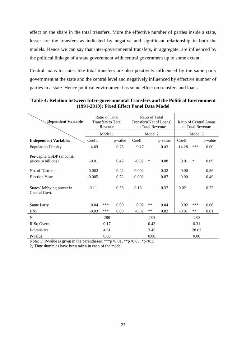
22

effect on the share in the total transfers. More the effective number of parties inside a state,

lesser are the transfers as indicated by negative and significant relationship in both the

models. Hence we can say that inter-governmental transfers, in aggregate, are influenced by

the political linkage of a state government with central government up to some extent.

Central loans to states like total transfers are also positively influenced by the same party

government at the state and the central level and negatively influenced by effective number of

parties in a state. Hence political environment has some effect on transfers and loans.

Table 4: Relation between Inter-governmental Transfers and the Political Environment

(1991-2010): Fixed Effect Panel Data Model

Dependent Variable

Independent Variables

Ratio of Total

Transfers to Total

Revenue

Ratio of Total

Transfers(Net of Loans)

to Total Revenue

Ratio of Central Loans

to Total Revenue

Model 1 Model 2 Model 5

Coeff. p-value Coeff. p-value Coeff. p-value

Population Density -4.69

0.75 9.17

0.43 -14.28 *** 0.00

Per-capita GSDP (at const.

prices in billions) -0.01

0.42 -0.02 * 0.08 0.01 * 0.09

No. of Districts 0.002

0.42 0.002

0.32 0.00

0.86

Election Year -0.005

0.72 -0.002

0.87 -0.00

0.49

States’ lobbying power in

Central Govt.

-0.11 0.56 -0.13 0.37 0.02 0.72

Same Party 0.04 *** 0.00 0.02 ** 0.04 0.02 *** 0.00

ENP -0.03 *** 0.00 -0.02 ** 0.02 -0.01 ** 0.01

N 280 280 280

R-Sq Overall 0.17 0.43 0.31

F-Statistics 4.61 3.45 28.63

P-value 0.00 0.00 0.00

Note: 1) P-value is given in the parentheses. ***p<0.01, **p<0.05, *p<0.1;

2) Time dummies have been taken in each of the model.

23

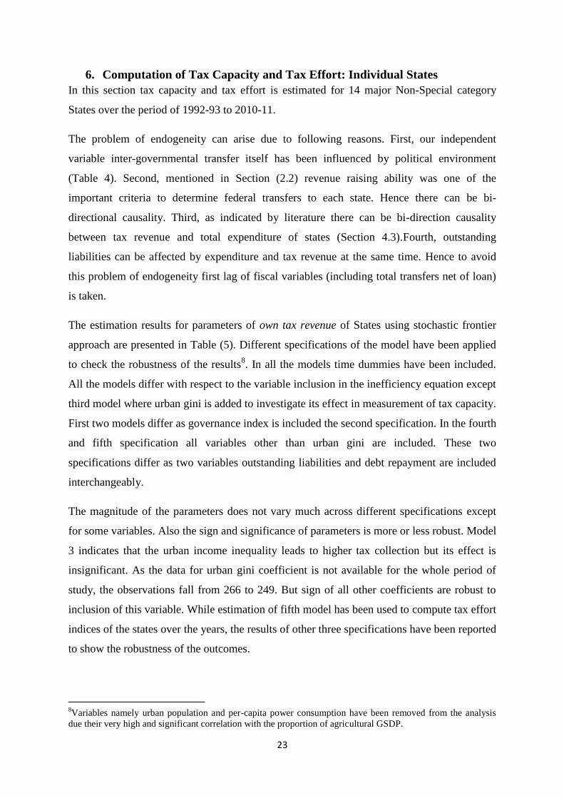
6. Computation of Tax Capacity and Tax Effort: Individual States

In this section tax capacity and tax effort is estimated for 14 major Non-Special category

States over the period of 1992-93 to 2010-11.

The problem of endogeneity can arise due to following reasons. First, our independent

variable inter-governmental transfer itself has been influenced by political environment

(Table 4). Second, mentioned in Section (2.2) revenue raising ability was one of the

important criteria to determine federal transfers to each state. Hence there can be bi-

directional causality. Third, as indicated by literature there can be bi-direction causality

between tax revenue and total expenditure of states (Section 4.3).Fourth, outstanding

liabilities can be affected by expenditure and tax revenue at the same time. Hence to avoid

this problem of endogeneity first lag of fiscal variables (including total transfers net of loan)

is taken.

The estimation results for parameters of own tax revenue of States using stochastic frontier

approach are presented in Table (5). Different specifications of the model have been applied

to check the robustness of the results8. In all the models time dummies have been included.

All the models differ with respect to the variable inclusion in the inefficiency equation except

third model where urban gini is added to investigate its effect in measurement of tax capacity.

First two models differ as governance index is included the second specification. In the fourth

and fifth specification all variables other than urban gini are included. These two

specifications differ as two variables outstanding liabilities and debt repayment are included

interchangeably.

The magnitude of the parameters does not vary much across different specifications except

for some variables. Also the sign and significance of parameters is more or less robust. Model

3 indicates that the urban income inequality leads to higher tax collection but its effect is

insignificant. As the data for urban gini coefficient is not available for the whole period of

study, the observations fall from 266 to 249. But sign of all other coefficients are robust to

inclusion of this variable. While estimation of fifth model has been used to compute tax effort

indices of the states over the years, the results of other three specifications have been reported

to show the robustness of the outcomes.

8Variables namely urban population and per-capita power consumption have been removed from the analysis

due their very high and significant correlation with the proportion of agricultural GSDP.

24

Tax collection is positively and significantly related with per-capita GSDP suggesting that

larger tax base as shown by higher per-capita GSDP leads to higher tax collection. One

percentage change in per-capita GSDP leads to 2.01 percent change in tax-GSDP ratio

(Model 5).The square term of this variable is negative and statistically significant in all five

models. Hence at higher levels of per-capita GSDP the elasticity of tax-GSDP ratio declines

suggesting that tax-GSDP ratio increases at decreasing rate. The coefficient of share of

agriculture GSDP is negative and statistically significant in all the models as expected. This

negative relationship suggests that large size of agriculture sector has negative impact on tax

collection which could be due to exemptions and lower incomes in this sector. Literacy rate, a

sign of development and awareness, has a positive and significant association with tax-GSDP

ratio in the fifth model. It could be due to higher incomes or compliance among literate

population. Hence literacy rate is an important variable to explain the taxation capacity of a

state. The proportion of labor force displays a positive and significant association with tax-

GSDP ratio in all the models. Larger labor force improves the tax base which further leads to

higher tax collection. Same holds true for road density which represents infrastructure

availability and has positive and significant association with tax-GSDP ratio.

6.1. Interpreting the Inefficiency Equation9

It turns out that in all five models the lambda parameter is statistically significant, which

indicates the presence of technical inefficiency. We estimate technical inefficiency after

controlling for real per-capita GSDP, structural variables like share of agricultural sector, and

economic variables like literacy rate, road length and labour force that affect tax potential of a

state. Next, we include a number of variables affecting technical inefficiency itself. The sign

and significant of the parameters in inefficiency equation is robust to inclusion or exclusion

of variables. In all the specifications, effect of fiscal variables indicated that the central

transfers to States are positively and significantly related with the inefficiency in tax

collection which indicates that central transfers up to some extent substitute States’ own tax

collection. One percentage point increase in central transfers (net of loan) to total revenue

receipts ratio leads to 1.80 percentage point increase in the inefficiency (model 5). The sign

and significance of this parameter is robust to inclusion of other variables in rest of the

models.

9 The dependent variable in inefficiency equation is the Tax Inefficiency. The coefficients in this equation are

also interpreted as effect on efficiency. Hence variables with positive (negative) effect on inefficiency are

explained to have negative (positive) effect on efficiency.

25

Table 5: Simultaneous Estimation of Tax Revenue and Technical Inefficiency: Stochastic Frontier Approach (1992-93 to 2010-11)

Dependent Variable: ln (Ratio of Total Own Tax

Revenue to GSDP)

Model 1 Model 2 Model 3 Model 4 Model 5

Coeff. p-value Coeff. p-value Coeff. p-value Coeff. p-value Coeff. p-value

Ln PC Real GSDP 2.39*** 0.00 1.97*** 0.00 2.82*** 0.00 1.51*** 0.00 2.01*** 0.00

Sq (Ln PC Real GSDP) -0.14*** 0.00 -0.12*** 0.00 -0.17*** 0.00 -0.09*** 0.00 -0.12*** 0.00

Ln (Agriculture share in GSDP) -0.06* 0.07 -0.07** 0.04 -0.07** 0.02 -0.06** 0.04 -0.07** 0.02

Ln (Literacy Rate) 0.09 0.45 0.29** 0.02 0.09 0.36 0.24** 0.03 0.24** 0.04

Ln(Labor Force) 0.35*** 0.00 0.28*** 0.00 0.51*** 0.00 0.25*** 0.00 0.20** 0.02

Ln(Road Density) 0.03* 0.07 0.02 0.25 0.06*** 0.00 0.04** 0.01 0.04** 0.03

Ln (Urban gini)

0.11 0.18

Constant

-

13.64*** 0.00 -12.08*** 0.00 -16.15*** 0.00 -9.90*** 0.00

-

12.00*** 0.00

Inefficiency Equation

(Ratio of Transfers net of loan to Rev. Receipts)t-1 2.21*** 0.00 1.84*** 0.00 2.53*** 0.00 2.00*** 0.00 1.80*** 0.00

(Ratio of Total Expenditure to GSDP(current)) t-1

-1.84*** 0.00 -1.50*** 0.00 -2.32*** 0.00

(Ratio of Outstanding Liabilities to GSDP(current)) t-1

0.66*** 0.00

(Ratio of Debt Repay to Total Rev) t-1

0.39*** 0.00

(Governance Index) t-1

-0.06*** 0.00 -0.03** 0.04 -0.04*** 0.00 -0.04*** 0.00

FRBMA -0.12*** 0.00 -0.10*** 0.00 -0.06* 0.09 -0.07** 0.02 -0.05* 0.09

ENP -0.04*** 0.01 -0.04*** 0.00 -0.06*** 0.00 -0.04*** 0.00 -0.04*** 0.01

State Govt. Share in Central Govt. -0.13 0.58 0.08 0.71 0.06 0.80 0.00 0.99 0.07 0.75

Election Year 0.01 0.57 0.02 0.37 0.01 0.63 0.01 0.55 0.02 0.33

Same Party -0.01 0.80 -0.01 0.77 0.03 0.15 0.01 0.52 0.01 0.66

Constant -0.38*** 0.00 -0.26*** 0.00 -0.14* 0.08 -0.20*** 0.01 -0.10 0.17

N 266 266 249 266 266

Log-Likelihood 208.8 218.9 231.5 241.2 240.7

sigma_u 0.08*** 0.00 0.06*** 0.01 0.11*** 0.00 0.05** 0.01 0.06** 0.04

sigma_v 0.09*** 0.00 0.09*** 0.00 0.04*** 0.00 0.09*** 0.00 0.09*** 0.00

Lambda 0.94*** 0.00 0.68*** 0.00 2.50*** 0.00 0.52*** 0.00 0.68*** 0.00

Note: 1) P-value is given in the parentheses. ***p<0.01, **p<0.05, *p<0.1;

2) Time dummies have been taken in each of the model.

26

Proportion of expenditure to GSDP has negative and significant impact on inefficiency as

expected. One percentage point increase in total expenditure to GSDP ratio leads to -2.32

percentage point decrease in the inefficiency. Larger expenditure responsibilities of a

government call for more tax collection and hence less technical inefficiency in tax

collection.

Comparing fourth and fifth model we can see that the outstanding liabilities and debt

repayment both raise inefficiency of states. While one percentage point increase in debt

repayment to total revenue ratio leads to 0.39 percentage point increase in the inefficiency,

same increase in outstanding liabilities increase inefficiency by 0.66 percentage points.

Hence debt repayment causes lesser inefficiency than outstanding liabilities as indicated by

lower magnitude of the coefficient. This might indicate the positive effect of an attempt to

improve state finances.

The governance index has negative and significant impact on inefficiency in tax collection. It

implies that better governance in general reduces inefficiency in tax collection by States.

Econometric analysis also reveals that FRBMA Act, which is aimed to achieve fiscal

discipline among states, has contributed to reduce their inefficiency in tax collection.

While observing the effect of political environment on tax inefficiency, only one variable,

effective number of political parties (ENP), effects tax inefficiency with negative and

significant sign. More competition among political parties may be making them more

accountable and efficient, raising tax effort of the state government. Other variables do not

have any significant effect on the inefficiency in tax collection, although we saw that other

political variables affect transfers (with and without central loans) that in turn affect tax

effort.

6.2. Tax Effort Index

The fifth model from Table (5) has been chosen to compute the tax effort. Table (6) reports

the estimates of tax effort scores and ranks of states for the years 1992, 2001 and 2010.

Figure (2) presents state-wise trends in tax efficiency score during the period 1992 to 2010

and Table (7) presents the comparison of tax efficiency score before and after the

implementation of FRBMA.

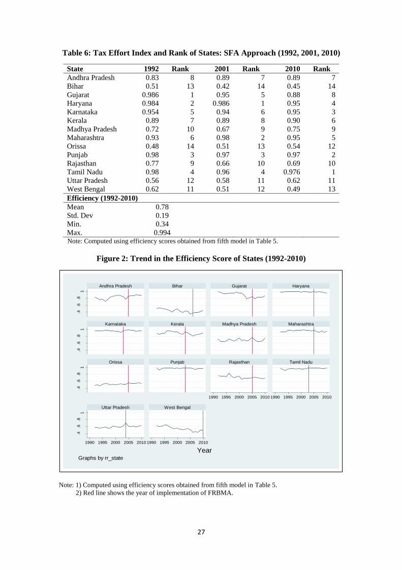
27

Table 6: Tax Effort Index and Rank of States: SFA Approach (1992, 2001, 2010)

State 1992 Rank 2001 Rank 2010 Rank

Andhra Pradesh 0.83 8 0.89 7 0.89 7

Bihar 0.51 13 0.42 14 0.45 14

Gujarat 0.986 1 0.95 5 0.88 8

Haryana 0.984 2 0.986 1 0.95 4

Karnataka 0.954 5 0.94 6 0.95 3

Kerala 0.89 7 0.89 8 0.90 6

Madhya Pradesh 0.72 10 0.67 9 0.75 9

Maharashtra 0.93 6 0.98 2 0.95 5

Orissa 0.48 14 0.51 13 0.54 12

Punjab 0.98 3 0.97 3 0.97 2

Rajasthan 0.77 9 0.66 10 0.69 10

Tamil Nadu 0.98 4 0.96 4 0.976 1

Uttar Pradesh 0.56 12 0.58 11 0.62 11

West Bengal 0.62 11 0.51 12 0.49 13

Efficiency (1992-2010)

Mean 0.78

Std. Dev 0.19

Min. 0.34

Max. 0.994 Note: Computed using efficiency scores obtained from fifth model in Table 5.

Figure 2: Trend in the Efficiency Score of States (1992-2010)

Note: 1) Computed using efficiency scores obtained from fifth model in Table 5.

2) Red line shows the year of implementation of FRBMA.

.4.6

.81

.4.6

.81

.4.6

.81

.4.6

.81

1990 1995 2000 2005 2010 1990 1995 2000 2005 2010

1990 1995 2000 2005 2010 1990 1995 2000 2005 2010

Andhra Pradesh Bihar Gujarat Haryana

Karnataka Kerala Madhya Pradesh Maharashtra

Orissa Punjab Rajasthan Tamil Nadu

Uttar Pradesh West Bengal

Eff

icie

ncy S

core

YearGraphs by rr_state

28

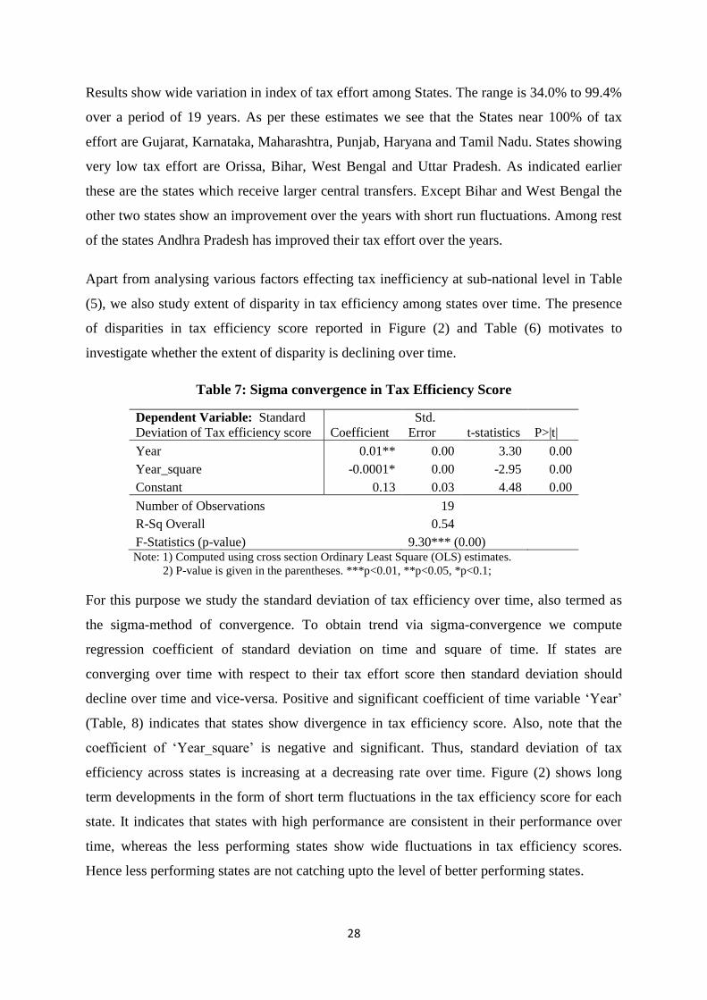
Results show wide variation in index of tax effort among States. The range is 34.0% to 99.4%

over a period of 19 years. As per these estimates we see that the States near 100% of tax

effort are Gujarat, Karnataka, Maharashtra, Punjab, Haryana and Tamil Nadu. States showing

very low tax effort are Orissa, Bihar, West Bengal and Uttar Pradesh. As indicated earlier

these are the states which receive larger central transfers. Except Bihar and West Bengal the

other two states show an improvement over the years with short run fluctuations. Among rest

of the states Andhra Pradesh has improved their tax effort over the years.

Apart from analysing various factors effecting tax inefficiency at sub-national level in Table

(5), we also study extent of disparity in tax efficiency among states over time. The presence

of disparities in tax efficiency score reported in Figure (2) and Table (6) motivates to

investigate whether the extent of disparity is declining over time.

Table 7: Sigma convergence in Tax Efficiency Score

Dependent Variable: Standard

Deviation of Tax efficiency score Coefficient

Std.

Error t-statistics P>|t|

Year 0.01** 0.00 3.30 0.00

Year_square -0.0001* 0.00 -2.95 0.00

Constant 0.13 0.03 4.48 0.00

Number of Observations 19

R-Sq Overall 0.54

F-Statistics (p-value) 9.30*** (0.00) Note: 1) Computed using cross section Ordinary Least Square (OLS) estimates.

2) P-value is given in the parentheses. ***p<0.01, **p<0.05, *p<0.1;

For this purpose we study the standard deviation of tax efficiency over time, also termed as

the sigma-method of convergence. To obtain trend via sigma-convergence we compute

regression coefficient of standard deviation on time and square of time. If states are

converging over time with respect to their tax effort score then standard deviation should

decline over time and vice-versa. Positive and significant coefficient of time variable ‘Year’

(Table, 8) indicates that states show divergence in tax efficiency score. Also, note that the

coefficient of ‘Year_square’ is negative and significant. Thus, standard deviation of tax

efficiency across states is increasing at a decreasing rate over time. Figure (2) shows long

term developments in the form of short term fluctuations in the tax efficiency score for each

state. It indicates that states with high performance are consistent in their performance over

time, whereas the less performing states show wide fluctuations in tax efficiency scores.

Hence less performing states are not catching upto the level of better performing states.

29

7. Conclusion

Constitution divides the revenue and expenditure responsibilities between centre and state

governments. States’ own tax revenue is the one of the important tools to finance their

expenditure responsibilities. It constitutes sales tax; taxes on land revenue &agricultural

income; taxes on mineral rights; taxes on profession, trades, & callings; and taxes on the

consumption of electricity etc. Sales tax is an indirect tax and forms the majority of revenue

of Indian states. This paper empirically estimates the own tax capacity and tax effort of 14

Indian states for the period of 1992-2010 using SFA and a comprehensive panel data set. SFA

is an improvement over traditional approaches to measure tax capacity such as RTS and

aggregate regression approach. It allows us not only to compute the tax effort index but also

to study the factors affecting tax inefficiency. The present study also uses comprehensive data

on factors which can be broadly put in following categories: structural variables, political

variables, economic variables and governance variables. Tax effort index is constructed to

measure the gap between estimated tax capacity and actual tax revenue. While tax capacity is

the maximum potential tax revenue that a government can generate, tax effort indicates what

part of maximum potential revenue a state has generated. Our results indicate that the tax

capacity is influenced not only by its tax base but also by economic, demographic,

infrastructure, political variables, index for administration & governance and fiscal incentive

variables. Different models are estimated to ensure robustness of the results.

Variables included have expected effect on the tax collection of the states. Tax revenue varies

positively and significantly with the per capita GSDP (in real terms) which is considered as

tax base for states. But share of agriculture adversely effects the tax collection. Variables like

labour force, literacy rate and infrastructure have positive and significant influence on tax

collection.

There is large variation in tax effort of individual states. States with consistently higher level

of tax efficiency are Haryana, Punjab, Karnataka, Kerala and Maharashtra. Low tax

efficiency score was observed in Bihar, Orissa, Uttar Pradesh and West Bengal. Inequality in

tax efficiency among states, measured by standard deviation, has increased over time.

Tax effort/efficiency of a state is adversely influenced by the magnitude of transfers it

receives from the central government. In other words these transfers substitute the own tax

collection of a state up to some extent. Higher outstanding liabilities of a state also have an

adverse effect on tax efficiency. Effect of debt repayment is also adverse but is less adverse

30

as compared to the effect of outstanding liabilities, implying reducing dependence on union

transfers and efforts to reduce the outstanding liabilities over time would increase tax effort.

Higher government expenditure has a favourable effect on tax efficiency. Among other

variables, law and order index, considered as a proxy for administration and governance, has

a favourable effect on tax efficiency. Although the large size of agricultural sector reduces

overall tax collection, high literacy rate and infrastructural facilities increase tax collection.

Implementation of FRBMA has had a favourable effect on tax efficiency. During TWFC

fiscal incentives in terms of availing DCRF and debt write off facility to state governments

were made conditional upon implementation of FRBMA and all state governments were

given autonomy to design their FRLs. As tax efficiency shows better results during FRBMA

regime, hence we can say that FRBMA, a self-sustaining rule which aims to bring down

primary & fiscal deficit and reduce the debt liabilities, has helped states improve their tax

collection.

Political variables did not give conclusive results, although the effective number of parties

with respect to seats won, which indicates political competition inside a state, has a

favourable effect on the tax efficiency. But the same party at the centre and the state tends to

increase transfers to states, and the latter reduces tax efficiency. States with more political

competition have a better tax effort. Decreasing the centre’s discretion would also improve

states tax effort.

There exists disparity in tax effort across states and it is widening over time. Conditional

benefits of DCRF and the debt write-off scheme attached with implementation of FRBMA

improved the tax effort of states, but the absence of convergence suggests these effects have

not been large enough. Therefore the elements of conditional transfers and debt write offs

should be increased in future Finance Commission awards. Since more development, better

infrastructure and governance improve tax effort, transfers can also be made conditional on

expenditure in areas like health, education, sanitation, and infrastructure that contribute to

development. This would also help the Finance Commission move back to its original

constitutional mandate of providing uniform public services through the country. The

imposition of planning soon after independence led to a dilution of this mandate (Goyal,

2013).

Transfers have to be accompanied by discipline otherwise they motivate the weaker states to

remain weak and underprovide the public services the transfers are made to finance. Such

31

conditionality should also accompany other types of transfers, even as the share of

discretionary transfers is reduced. This would also increase the share of formula based

transfers such as the Finance Commissions award. Incentive mechanisms work best when

isolated from political renegotiation. The Centre should absorb less of the risk of market

borrowings by states, so market discipline also contributes. One of our results is larger

expenditure responsibilities are followed by higher tax effort. To the extent conditional

transfers maintain expenditure their effect on weakening expenditure and lowering tax effort

would be reduced. More research is required on the extent to which states met FRBM targets

by reducing expenditure, and how to ring fence productive expenditure.

Conditionality in transfers can reduce freedoms for states. At present tight restrictions on end

use and delays in sanctions reduce the utility of the transfers for states. But conditionality and

better local projects are consistent if transfers are made more time-bound and outcome rather

than use based. The changes have to be gradual and in step with local capacity creation to

deliver outcomes.

Strengthening of factors associated with better tax collection is a long term process.

Nevertheless a sharper identification of the variables that affect these factors, allows policies

to better target these variables, so that improvements, such as in per-capita GSDP which is

the overall tax base, take place faster.

32

References

Advisory Commission on Intergovernmental Relations (ACIR) (1962): Measure of State and

Local Fiscal Capacity and Tax Effort, Report No. M-16, October, Washington DC, USA.

Available at: http://www.library.unt.edu/gpo/acir/Reports/information/M-16.pdf

Aigner, D. J., Lovell, Knox, C.A. and Schmidt, P. (1977): “Formulation and Estimation of

Stochastic Frontier Production Function Models”, Journal of Econometrics, 6, pp. 21-37.

Alfirman, L. (2003): “Estimating Stochastic Frontier Tax Potential: Can Indonesian Local

Governments Increase Tax Revenues under Decentralization”, Working paper no. 03-19,

Center for Economic Analysis, Dept. of Economics, University of Colorado.

Arulampalam, W. et. al. (2008): “Electoral Goals and Centre-State Transfers: A Theoretical

Model and Empirical Evidence from India”, Journal of Development Economics, Vol. 88,

Issue 1, pp. 103-119.

Bagchi, A. (2003): Fifty Years of Fiscal Federalism in India, An Appraisal, Working paper

No. 02, NIPFP, New Delhi.

Bahl, R. W. (1972): A Representative Tax System Approach to Measuring Tax Effort in

Developing Countries, Staff Papers, IMF, Vol. 19, No. 1, pp. 87-124.

Battese, G., and Coelli, T. (1995): “A Model for Technical Inefficiency Effects in a

Stochastic Frontier Production Function for Panel Data”, Empirical Economics, 20, pp.

325−332.

Bhargava, P. K. (1999): “Reforms ion Taxation of Agricultural Income in India”, in Financial

Sector Reforms, Tax System and Development- Experiences and Challenges, ed. D. K. Das,

The Indian Economic Association, New Delhi.

Biswas, R. et. al. (2010): “Fiscal Federalism, State Lobbying and Discretionary Finance:

Evidence from India”, Economics & Politics, Vol. 22, Issue 1, pp. 68-91.

Chatterjee, P. (1968): “Agriculture Income-Tax Some Relevant Issues”, Economic and

Political Weekly, Vol. 3, No. 29.

Cyan, M. et. al.(2013): Measuring Tax Effort: Does the Estimation Approach Matter and

Should Effort be Linked to Expenditure Goals, Working Paper, International Center for

Public Policy.

Das, S. et. al.(2010): “Regional Convergence of Growth, Inequality and Poverty in India-An

Empirical Study”, Economic Modelling, 27, pp.1054-1060.

Dash, B. B. and A. V. Raja (2009): “Institutions and the Quality of Governance: An

Empirical Study on Interstate Differences in Economic Development in India”, Asia-Pacific

Developmental Journal, Vol. 16, Issue 1, pp. 1-26.

Dash, B. B. and A. V. Raja (2013): “Intergovernmental Transfers and Tax Collection in

India: Does the Composition of Transfers Matter?”, Public Budgeting and Finance, Vol. 33,

Issue 2, pp. 93-116.

33

Davoodi, H. and D. Grigorian (2007): Tax Potential vs. Tax Effort: A Cross-Country Analysis

of Armenia’s Stubbornly Low Tax Collection, Working Paper, International Monetary Fund,

WP/07/106.

Finance Commission (2000): Report of the Eleventh Finance Commission (2000-2005),

Government of India, New Delhi.

Finance Commission (2004): Report of the Twelfth Finance Commission (2005-2010),

Government of India, New Delhi.

Finance Commission (2009): Report of the Thirteenth Finance Commission (2010-2015),

Government of India, New Delhi.

Government of West Bengal (2011): The West Bengal Fiscal Responsibility and Budget

Management Act, 2010, Finance Department, West Bengal. Available at:

http://www.wbfin.nic.in/writereaddata/Budget_Publication/FRBM%2812-13%29.pdf

Goyal, A. (2013): Sustaining growth: Interests versus institutions, Working Paper, IGIDR,

WP-2013-001.

Gupta, A. (2007): Determinants of Tax Revenue Efforts in Developing Countries, Working

Paper, International Monetary Fund, WP/07/184.

Jha, R.et. al. (1999): “Tax Efficiency in Selected Indian States”, Empirical Economics, 24:

641-654.

Ho, Y. H. and C. J. Huang (2009): “Tax-Spend, Spend-Tax, or Fiscal-Synchronization: A

Panel Analysis of the Chinese Provincial Real Data”, Journal of Economics and

Management, Vol. 5, No. 2, pp. 257-272.

Kaushik, A. and R. Pal (2012): Political Strongholds and Budget Allocation for

Developmental Expenditure: Evidence from Indian States, 1971-2005, Working Paper,

IGIDR, WP-2012-015.

Krishna, R. (1972): “Inter-sectoral Equity and Agricultural Taxation in India”, Economic and

Political Weekly, Vol. 7, No. 31-32-33.

Mahdavi, S. (2013): State Government Tax Revenue, Tax Revenue Composition and Tax

Effort Index: An Assessment of the 1978-97 Period, Working Paper, The University of Texas

at San Antonio, 0036ECO-090-2013.

Misra, B. M. and J. K. Khundrakpam (2009): Fiscal Consolidation by Central and State

Governments: The Medium Term Outlook, RBI Staff Studies.

Mundle, S. et. al. (2012): The quality of governance: How have Indian States Performed?,

Working Paper No. 2012-104, NIPFP, New Delhi.

Naganathan, M. and K. J. Sivagnanam (2000): “Federal Transfers and Tax Efforts of States in

India”, The Indian Economic Journal, Vol. 47, No. 4, pp. 101-10.

Oommen, M. A. (1987): “Relative Tax Effort of States”, Economic and Political Weekly,

Vol. 22, No. 11, pp. 466-470.

34

Panda, P. K. (2009): “Central Fiscal Transfers and States’ Own-Revenue Efforts in India:

Panel Data Models”, The Journal of Applied Economic Research, Vol. 3, No. 3, pp. 223-242.

Pessino, C. and R. Fenochietto (2010): “Determining Countries’ Tax Effort,” Hacienda

Pública Española/Revista de Economía Pública, Vol. 195, pp. 61–68.

Pessino, C. and R. Fenochietto (2013): Understanding Countries’ Tax Effort, Working Paper,

Fiscal Affairs Department, International Monetary Fund, WP/13/244.

Piancastelli, M. (2001): Measuring the Tax Effort of Developed and Developing Countries:

Cross Country Panel Data Analysis-1985/95, IPEA Working Paper No. 818. Available at

SSRN: http://ssrn.com/abstract=283758 or http://dx.doi.org/10.2139/ssrn.283758

Planning Commission (2004): Finance of State Governments in India: Volume I & II.

Available at: http://planningcommission.nic.in/reports/sereport/ser/statfins/sty_statefins.htm

Planning Commission (2012): Report of the Working Group on States’ Financial Resources

for Twelfth Five Year Plan (2012-2017), Planning Commission, Government of India, New

Delhi.

Purohit, M. C. (2006): “Tax Efforts and Taxable Capacity of Central and State

Governments”, Economic and Political Weekly, Vol. 41, No. 8, pp. 747-751+753-755.

Ramalingom, R. and K. N. Kurup (1991): “Plan Transfers to States: Revised Gadgil Formula:

An Analysis”, Economic and Political Weekly, Vol. 26, No. 9/10, pp. 501-506.

Rao, H. (1993): “Taxable Capacity Tax-Efforts and Forecasts of Tax-Yield of Indian States”,

ISEC. Available at

http://203.200.22.249:8080/jspui/bitstream/123456789/45/1/Taxable_capacity_for_tax_effort

s_and_forecast.pdf

Rao, M. G, R. T. Shand and K. P. Kalirajan (1999): “Convergence of Income across Indian

States: A Divergent View”, Economic and Political Weekly, Vol. 34, No. 13, pp. 769-778.

Rao, M. G. and N, Singh (2007): “The Political Economy of India’s Fiscal Federal System

and its Reform”, Publius, Vol. 37, No. 1, pp, 26-44.

Rao, M. G. and T. Sen (2011): Federalism and Fiscal Reform in India, Working Paper, No.

84, National Institute of Public Finance and Policy, New Delhi.

Reserve Bank of India (2004): Handbook of Statistics on State Government Finances.

Reserve Bank of India (2010): Handbook of Statistics on State Government Finances.

Reserve Bank of India (2012): State Finances: A Study of Budgets of 2011-12.

Sengupta, D. P. and R. K. Rao (2012): “Direct Taxes Code and Taxation of Agricultural

Income”, Economic and Political Weekly, Vol. 47, No. 15.

Simone, A. S. and Topalova, P. (2009): India’s Experience with Fiscal Rules: An Evaluation

and The Way Forward, Working Paper, No. 175, Asia and Pacific Department, International

Monetary Fund.

35

Singh, N. and G, Vasishtha (2004): Some Patterns in Centre-State Fiscal Transfers in India:

An Illustrative Analysis, Working paper, Santa Cruz Center for International Economics,

University of California.

Thimmaiah, G. (1979): Revenue Potential and Revenue Efforts of Southern States. A study

sponsored by the Planning Commission, Government of India, New Delhi.

36

Appendices

37

Table A1: Criteria of FC Transfers

Finance

Commission

Criteria Applicable to

Population Distance Inverse

of

Income

Poverty

Ratio

Index of

Backwardness

Area Index of

Infrastructure

Tax

Effort

Fiscal

Discipline

Fiscal

Capacity

Distance

Eighth 25 50 25 - - - - - - - 90% of Shareable

IT

Ninth (I

report)

25 50 12.5 12.5 - - - - - - 40% of UED

Ninth (II

report)

25 50 12.5 - 12.5 - - - - - 90% of Shareable

IT

29.94 40.12 14.97 - 14.97 - - - - - 37.575% of UED

Tenth 20 60 - - - 5 5 10 - - 100% of

Shareable IT and

40% of UED

Eleventh 25 50 - - - 10 - 7.5 7.5 - -

Twelfth 10 62.5 - - - 7.5 7.5 5 7.5 - -

Thirteenth 25 - - - - 10 - - 17.5 47.5 -

Source: Finance Commission (2000, 2004, 2009)

38

Table A2: Criteria for PC Transfers: Gadgil Formula

Criteria Modified Gadgil

Formula (1980)

NDC Revised

Formula (1990)

NDC Revised

Formula (1991)

A. Special Category States (10) 30% share of 10

States excluding

North Eastern

Council

30% share of 10

States including

North Eastern

Council

30% share of 10

States excluding

North Eastern

Council

B. General Category States (15)

(i) Population (1971) 60 55 60

(ii) Per Capita Income 20 25 25

Of which

a. According to the `deviation’ method

covering only the states with per capita

income below the national average 20 20 20

b. According to the `distance’ method

covering all the fifteen states - 5 5

(iii) Performance 10 5 7.5

Of which

a. Tax effort 10 - 2.5

b. Fiscal management - 5 2.5

c. National objectives - - 2.5

(iv) Special problems 10 15 7.5

Total 100 100 100 Notes: 1. Fiscal management is assessed as the difference between states’ own total plan resources estimated at

the time of finalizing Annual Plans and their actual performance, considering latest five years.

2. Under the criterion of the performance in respect of certain programmes of national priorities the

approved formula covers four objectives, viz.: (i) population control; (ii) elimination of illiteracy; (iii) on-time

completion of externally aided projects; and (iv) success in land reforms.

Source: PC(2012).

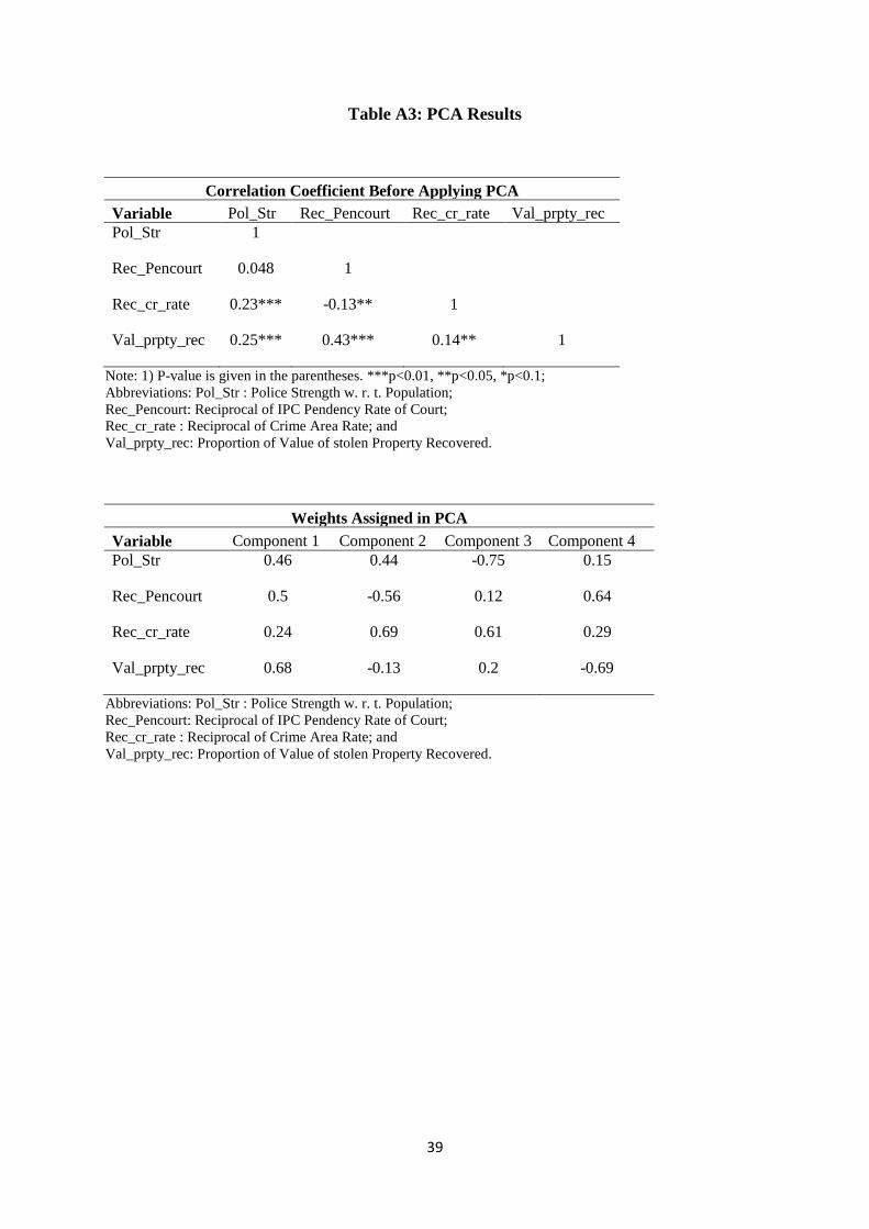
39

Table A3: PCA Results

Correlation Coefficient Before Applying PCA

Variable Pol_Str Rec_Pencourt Rec_cr_rate Val_prpty_rec

Pol_Str 1

Rec_Pencourt 0.048 1

Rec_cr_rate 0.23*** -0.13** 1

Val_prpty_rec 0.25*** 0.43*** 0.14** 1

Note: 1) P-value is given in the parentheses. ***p<0.01, **p<0.05, *p<0.1;

Abbreviations: Pol_Str : Police Strength w. r. t. Population;

Rec_Pencourt: Reciprocal of IPC Pendency Rate of Court;

Rec_cr_rate : Reciprocal of Crime Area Rate; and

Val_prpty_rec: Proportion of Value of stolen Property Recovered.

Weights Assigned in PCA

Variable Component 1 Component 2 Component 3 Component 4

Pol_Str 0.46 0.44 -0.75 0.15

Rec_Pencourt 0.5 -0.56 0.12 0.64

Rec_cr_rate 0.24 0.69 0.61 0.29

Val_prpty_rec 0.68 -0.13 0.2 -0.69

Abbreviations: Pol_Str : Police Strength w. r. t. Population;

Rec_Pencourt: Reciprocal of IPC Pendency Rate of Court;

Rec_cr_rate : Reciprocal of Crime Area Rate; and

Val_prpty_rec: Proportion of Value of stolen Property Recovered.

40

Table A4

State-wise Year of Implementation of FRBMA

State Year of Implementation of FRBMA

Andhra

Pradesh

October 2005

Bihar April 2006

Gujarat March 2005

Haryana July 2005

Karnataka August 2002 (came into force on April

2003)

Kerala September 2003

Madhya

Pradesh

August 2005

Maharashtra April 2005

Orissa May 2005

Punjab May 2003

Rajasthan May 2005

Tamil Nadu May 2003

Uttar Pradesh February 2004

West Bengal* 2010

Source: Misra and Khundrakpam (2009), RBI Staff Studies.

* Government of West Bengal (2011)

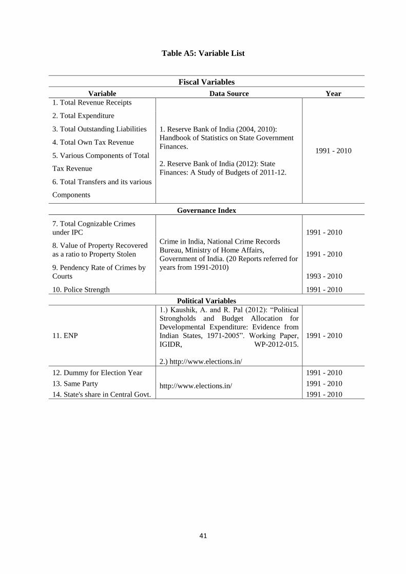
41

Table A5: Variable List

Fiscal Variables

Variable Data Source Year

1. Total Revenue Receipts

1. Reserve Bank of India (2004, 2010):

Handbook of Statistics on State Government

Finances.

2. Reserve Bank of India (2012): State

Finances: A Study of Budgets of 2011-12.

1991 - 2010

2. Total Expenditure

3. Total Outstanding Liabilities

4. Total Own Tax Revenue

5. Various Components of Total

Tax Revenue

6. Total Transfers and its various

Components

Governance Index

7. Total Cognizable Crimes

under IPC

Crime in India, National Crime Records

Bureau, Ministry of Home Affairs,

Government of India. (20 Reports referred for

years from 1991-2010)

1991 - 2010

8. Value of Property Recovered

as a ratio to Property Stolen 1991 - 2010

9. Pendency Rate of Crimes by

Courts 1993 - 2010

10. Police Strength 1991 - 2010

Political Variables

11. ENP

1.) Kaushik, A. and R. Pal (2012): “Political

Strongholds and Budget Allocation for

Developmental Expenditure: Evidence from

Indian States, 1971-2005”. Working Paper,

IGIDR, WP-2012-015.

2.) http://www.elections.in/

1991 - 2010

12. Dummy for Election Year

http://www.elections.in/

1991 - 2010

13. Same Party 1991 - 2010

14. State's share in Central Govt. 1991 - 2010

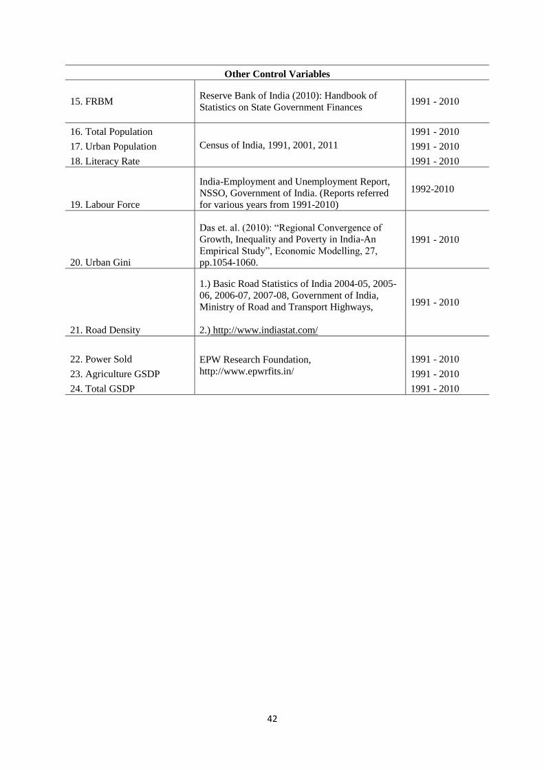
42

Other Control Variables

15. FRBM Reserve Bank of India (2010): Handbook of

Statistics on State Government Finances 1991 - 2010

16. Total Population

Census of India, 1991, 2001, 2011

1991 - 2010

17. Urban Population 1991 - 2010

18. Literacy Rate 1991 - 2010

19. Labour Force

India-Employment and Unemployment Report,

NSSO, Government of India. (Reports referred

for various years from 1991-2010)

1992-2010

20. Urban Gini

Das et. al. (2010): “Regional Convergence of

Growth, Inequality and Poverty in India-An

Empirical Study”, Economic Modelling, 27,

pp.1054-1060.

1991 - 2010

21. Road Density

1.) Basic Road Statistics of India 2004-05, 2005-

06, 2006-07, 2007-08, Government of India,

Ministry of Road and Transport Highways,

2.) http://www.indiastat.com/

1991 - 2010

22. Power Sold EPW Research Foundation,

http://www.epwrfits.in/

1991 - 2010

23. Agriculture GSDP 1991 - 2010

24. Total GSDP 1991 - 2010

43

List of Abbreviations

ACIR Advisory Commission on Intergovernmental Relations

CSS Centrally Sponsored Scheme

DCRF Debt Consolidation and Relief Facility

EFC Eleventh Finance Commission

FC Finance Commission

FRBMA Fiscal Responsibility and Budget Management Act

GDP Gross Domestic Product

GSDP Gross State Domestic Product

MTRFP Medium Term Fiscal Restructuring Policy

MP Member of Parliament

NDC National Development Council

NSSF National Social Security Fund

NSSO National Sample Survey Organisation

NCRB National Crime Records Bureau

NFC Ninth Finance Commission

NPG Non Planning Grant

PC Planning Commission

PCA Principal Component Analysis

RBI Reserve Bank of India

RTS Representative Taxation System

SFA Stochastic Frontier Analysis

TFC Tenth Finance Commission

THFC Thirteenth Finance Commission

TWFC Twelfth Finance Commission