Stochastic Production Frontier and TechnicalInefficiency : Evidence from Tunisian

Manufacturing Firms∗

RaÞk Baccouche�& Mokhtar Kouki� §

January 2002 (Preliminary version January 2000)

Abstract

In this paper, a stochastic frontier production model is estimatedon panel data, and technical inefficiency indices are computed forTunisian manufacturing Þrms over the 1983-1993 time period. Themost commonly used one-sided distributions of the inefficiency er-ror term are speciÞed, namely the truncated normal, the half-normaland the exponential distributions. A generalized version of the half-normal, which does not embody the zero-mean restriction, is also ex-plored. For each distribution, the likelihood function and the coun-terpart of Jondrow et al. (1982) estimator of technical efficiency areexplicitly stated. Based on our data set, formal tests lead to a strongrejection of the zero-mean restriction embodied in the half normaldistribution. Our main conclusion is that the degree of measured in-efficiency is very sensitive to the postulated assumptions about thedistribution of the one-sided error term. The estimated inefficiency

∗ We are acknowledged to Tahar Abdessalem, Jean Pierre Florens, Farouk Kriaa,Mohamed Salah Rejeb, Rached Bouaziz and Jean Charles Rochet for helpful commentsand suggestions. We are grateful to the �Secrétariat d�Etat à la Recherche ScientiÞque enTunisie� for the Þnancial support.

� University of Tunis 3.� LEGI - Polytechnics of Tunisia and University of Tunis§Correspondence to Mokhtar Kouki: LEGI - Polytechnics of Tunisia, BP743, 2048 La

Marsa Tunis - Tunisia. email: mokhtar.kouki@fsjegj.rnu.tn

1

indices are, however, unaffected by the choice of the functional formfor the production function.Keywords: Stochastic frontier; Farrell�s technical inefficiency; Unbal-anced panel data; Composed disturbance error; One-sided distribu-tion.

1 Introduction

The purpose of this paper is to estimate Þrm-speciÞc levels of technical in-efficiency using a panel data of Tunisian manufacturing Þrms. This paneldata set covers the time period 1983-1993. Our methodology applies thestochastic frontier analysis which became popular in the recent literature.The basic difference between stochastic frontier model and the standard

econometric model is that the former adds a one-sided distributed randomvariable to the usual stochastic disturbances term. This supplementary ran-dom variable is intended to take into account the amount by which observedoutput is less than potential output. This amount is a measure of technicalinefficiency in the sense of Farrell (1957).Econometric estimation of Þrm-speciÞc technical inefficiency raises two

problems. The Þrst problem relates to the appropriateness of the postulateddistribution for the one-sided error term, particularly if maximum likelihoodestimation method is to be used. Although an extensive literature had beendevoted to this question, the fact remains that there is little guidance asto the appropriate speciÞcation of the one-sided distribution. A sensitivityanalysis of the results to alternative distributional assumptions must then beconducted.Once the parameters of the model have been estimated, the second prob-

lem is how one can extract the inefficiency component from the estimatedcomposed error term. Jondrow et al. (1982) showed that Þrm-speciÞc esti-mates of inefficiency can be obtained through the distribution of the ineffi-ciency term conditional on the estimate of the whole composed error term.The Jondrow et al. estimator is easily seen to be inconsistent when usedwith a single cross-section. Consistency may, however, be achieved using apanel data of Þrms covering a sufficiently long time period.In our empirical work we consider three alternative distributions for the

one-sided error term, which are most commonly used by econometricians.These distributions are the truncated normal, the generalized half-normal

2

and the exponential distributions. The term �generalized� is used here todesignate the distribution of the absolute value of a non-zero mean normallydistributed variable. We are not aware of any empirical study which has usedthis distribution of which the standard half-normal (zero mean) is a specialcase.This paper is organized as follows. A brief discussion of some measure-

ment methods of technical inefficiency in the context of the stochastic frontiermodel is presented in the following section. In section 3, explicit formulas forthe log-likelihood functions and for the estimators of Þrm-speciÞc inefficiencyare given for the three distributions stated above, in the context of (unbal-anced) panel data. Section 4 presents data description and our empiricalresults. The main conclusions are summarized in section 5.

2 Stochastic Frontier Model and TechnicalInefficiency

The stochastic frontier model was introduced by Aigner, Lovell, and Schmidt(1977) and by Meeusen and Van der Broeck (1977) in order to avoid theshortcomings inherent to the deterministic frontier model1. It assumes acomposed error term reßecting both the usual statistical random noise andtechnical inefficiency. Assuming a log-linear form, the stochastic frontiermodel may be deÞned as follows

yit = α+ xitβ + εit, (1)

where yit and xit denote, respectively, the logarithms of observed output andof a row vector of inputs for the i th Þrm in the t th time period; α and βare the unknown parameters to be estimated and εit is the stochastic errorterm which is assumed to behave in a manner consistent with the stochasticfrontier concept, i.e.

²it = vit − ui. (2)

1The deterministic frontier model assumes only one-sided error term reßecting tech-nical inefficiency, so that any statistical noise due to misspeciÞcation of the model ormeasurement error in the variables will be translated into inefficiency.

3

The disturbances vit consist of random shocks in the production process be-yond the Þrms control and they are taken to be independent and identicallydistributed (i.i.d.) across observations as N (0, σ2

v). The random variables ui,which are assumed to be non-negative, reßect the shortfall of actual outputfrom the efficient frontier; they are also assumed to be i.i.d. as well as in-dependent of vit and of factor inputs. With this speciÞcation, the quantityeα+xitβ+vit speciÞes the efficiency stochastic production frontier as deÞned byAigner et al. (1977), while the case vit = 0 leads to the deterministic ef-Þciency frontier model in Aigner and Chu (1968). In either case technicalefficiency for each unit is measured by TEi = e−ui, which, as ui ≥ 0, liesbetween zero and one.The strength of the stochastic frontier is that it provides a method to

separate random disturbances caused by inefficiency in a Þrm�s behavior fromother uncontrolled random shocks. However, given that ui is not observable,direct estimation of TEi is not possible even when α and β are known.Computation of TEi requires prior estimation of the non-negative error

ui, i.e. a method of decomposition of the entire error term ε into its twoindividual components. Alternative solutions to this problem have been pro-posed in the recent literature, depending on whether we assume a particulardistribution for ui or not2. However, such a decision is heavily conditionedby the nature of inefficiency we are interested in, i.e. relative or absolute. Ifinefficiency is to be deÞned relative to a completely efficient base Þrm, thenno distributional assumption for ui is needed. In this case consistent residual-based estimation methods for Þrm-speciÞc inefficiency may be used as sug-gested by Greene (1980) in the case of a single cross-section, and Cornwellet al. (1990) for panel data. If, however, absolute Þrm-speciÞc inefficiency isto be computed, then prior assumption on the distribution of ui cannot beavoided. But, in such a case, only the population mean of technical ineffi-ciency, i.e. 1−E(TEi), may be calculated using the estimated parameters ofthe maintained distribution. IdentiÞcation of absolute Þrm-speciÞc technicalinefficiency is still impossible.To by-pass this problem, Jondrow et al. (1982), and Kalirajan and Flinn

(1983) propose to use the conditional expectation of ui, given the entire errorterm εi, as an estimator of Þrm-speciÞc technical inefficiency. This is veryattractive since such an estimator is also the best predictor of ui, i.e. the

2Greene (1994) offers an excellent survey of these methods. He also discusses the moregeneral case where technical inefficiency is time-variant. See, also Cornwell et al. (1990).

4

minimum mean-squared-error predictor. However, it must be noted that, inthe case of a single cross-section, this estimator is not consistent. This isbecause, while εi contains only imperfect information about ui, the varianceof the conditional distribution of ui given εi is independent of sample size.The variability of vi remains no matter how large N is. This deÞciency isresolved when panel data is used because the irrelevant variability containedin εit, i.e. vit, is being averaged over the number of periods T . So, consistentestimates of Þrm-speciÞc inefficiency may be obtained when T goes to inÞnity.Extension of Jondrow et al. predictor for use with panel data can be foundin Battese and Coelli (1988), Kumbhakar (1988), and Battese, Coelli andColby (1989).Much of the criticism addressed to the estimates of absolute technical in-

efficiency relate to the plausibility of the distributional assumption that mustbe made for the one-sided error term. Empirical studies, as in Greene (1980,1994) and Stevenson (1980) among many others, revealed that different spec-iÞed distributions do give different estimates of technical inefficiency. In somecases the estimates of the input coefficients were also affected. Without priorinformation on the economic processes generating the inefficiency, the choiceof any particular distribution cannot be justiÞed. In practice, such infor-mation is in general not available and different distributions must be triedin order to assess the sensitivity of the results to alternative distributionalspeciÞcations.Given that ui is a non-negative random variable, numerous density func-

tions can be speciÞed for it. Some distributions are however more attractivethan others. The half-normal, exponential and truncated-normal distribu-tions are by far the most used distributions in empirical studies. As pointedout by Stevenson (1980), the major drawback of the Þrst two distributionsis to restrict the density of the inefficiency to be most concentrated nearzero. This implies that �the likelihood of inefficient behavior monotonicallydecreases for increasing levels of inefficiency� 3. Stevenson proposed insteada more ßexible distribution of the inefficiency given by the truncated normaldensity function which does not restrict the mode to occur at zero. This isa natural extension in so far as it enables the testing of the adequacy of thezero-mode restriction4.

3See Stevenson (1980), p. 58.4Note that LM tests for the adequacy of the half-normal and truncated normal dis-

tributions have been explicitly derived by Lee (1983) conditional on the assumption thatthe distribution of ui belongs to the Pearson family of truncated distributions.

5

3 Alternative SpeciÞcations and ML Estima-tion

Prior to the computation of Þrm-speciÞc inefficiency the unknown parametersof the production function must be estimated. Note that, apart from theasymmetry of the distribution of ε, equations (1) and (2) Þt well into thestandard random effects model in panel data literature. The asymmetrycharacterizing εit doesn�t matter, and in any case it can be easily avoided byadjusting the constant term α.The choice of the method of estimation must be assessed according to

some basic assumptions concerning the disturbances term. For example,assuming exogenous factor inputs, the Feasible GLS technique may be usedto derive consistent estimates of the frontier. The main advantage of thistechnique is that no distributional speciÞcation is needed for the one-sidederror term for consistent estimates of the parameters. However, assumingthe distribution of ui to be known, some efficiency gain over GLS may beachieved through the ML method. If factor inputs were to be correlated withthe disturbances then neither GLS nor ML estimator would be consistent.In such a case, an efficient IV estimator of the type discussed by Hausmanand Taylor (1981) must be used5. Recall however, that, given the parametersestimates, prior knowledge of the inefficiency distribution is required whenabsolute Þrm-speciÞc inefficiency is sought.In this study, we choose to focus attention exclusively on the MLEmethod

in estimating the production frontier parameters. We use three differentspeciÞcations for the distribution of ui. These are the truncated normal,the generalized half-normal and the exponential distributions. The Þrst twodistributions are general enough in that they do not restrict the mode to occurat zero, and they both encompass the standard half-normal as a special case.Before going to the results, we give in the following the explicit formulas

we used in our programming procedures. These formulas are stated for thegeneral case of unbalanced panel data, and encompass both the productionfrontier and the cost frontier cases. Indeed, as we deÞne εit = vit+δui, whereδ is a switching parameter taking value of −1 for a production frontier andvalue of 1 for a cost frontier, we can move from one speciÞcation to anotherby assigning an appropriate value to δ wherever it appears.In deriving our results, the following two assumptions are made: (i) the

5See, Schmidt and Sickles (1984), and Cornwell et al. (1990).

6

random variables vit are assumed to be i.i.d. across observations as N(0, σ2v),

as well as independent of the ui random variables, (ii) vit and ui are bothassumed to be independently distributed of the factor inputs in the model6.

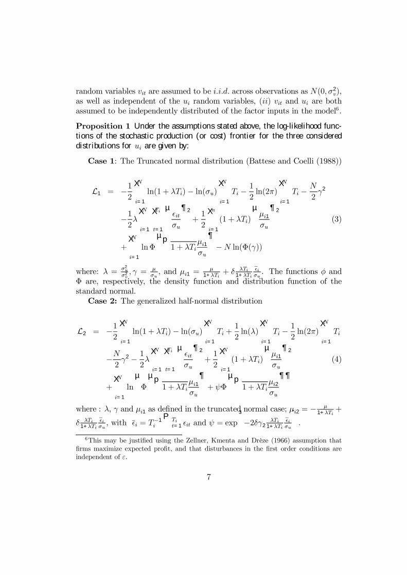
Proposition 1 Under the assumptions stated above, the log-likelihood func-tions of the stochastic production (or cost) frontier for the three considereddistributions for ui are given by:

Case 1: The Truncated normal distribution (Battese and Coelli (1988))

L1 = −12

NXi=1

ln(1 + λTi)− ln(σu)NXi=1

Ti − 12ln(2π)

NXi=1

Ti − N2γ2

−12λ

NXi=1

TiXt=1

µ²itσu

¶2

+1

2

nXi=1

(1 + λTi)

µµi1σu

¶2

(3)

+

NXi=1

lnΦ

µp1 + λTi

µi1σu

¶−N ln(Φ(γ))

where: λ = σ2u

σ2v, γ = µ

σu, and µi1 =

µ1+λTi

+ δ λTi1+λTi

²̄iσu. The functions φ and

Φ are, respectively, the density function and distribution function of thestandard normal.Case 2: The generalized half-normal distribution

L2 = −12

NXi=1

ln(1 + λTi)− ln(σu)NXi=1

Ti +1

2ln(λ)

NXi=1

Ti − 12ln(2π)

NXi=1

Ti

−N2γ2 − 1

2λ

NXi=1

TiXt=1

µ²itσu

¶2

+1

2

NXi=1

(1 + λTi)

µµi1σu

¶2

(4)

+NXi=1

ln

µΦ

µp1 + λTi

µi1σu

¶+ ψΦ

µp1 + λTi

µi2σu

¶¶where : λ, γ and µi1 as deÞned in the truncated normal case; µi2 = − µ

1+λTi+

δ λTi1+λTi

²̄iσu, with ²̄i = T

−1i

PTit=1 ²it and ψ = exp

³−2δγ2

λTi1+λTi

²̄iσu

´.

6This may be justiÞed using the Zellner, Kmenta and Drèze (1966) assumption thatÞrms maximize expected proÞt, and that disturbances in the Þrst order conditions areindependent of ε.

7

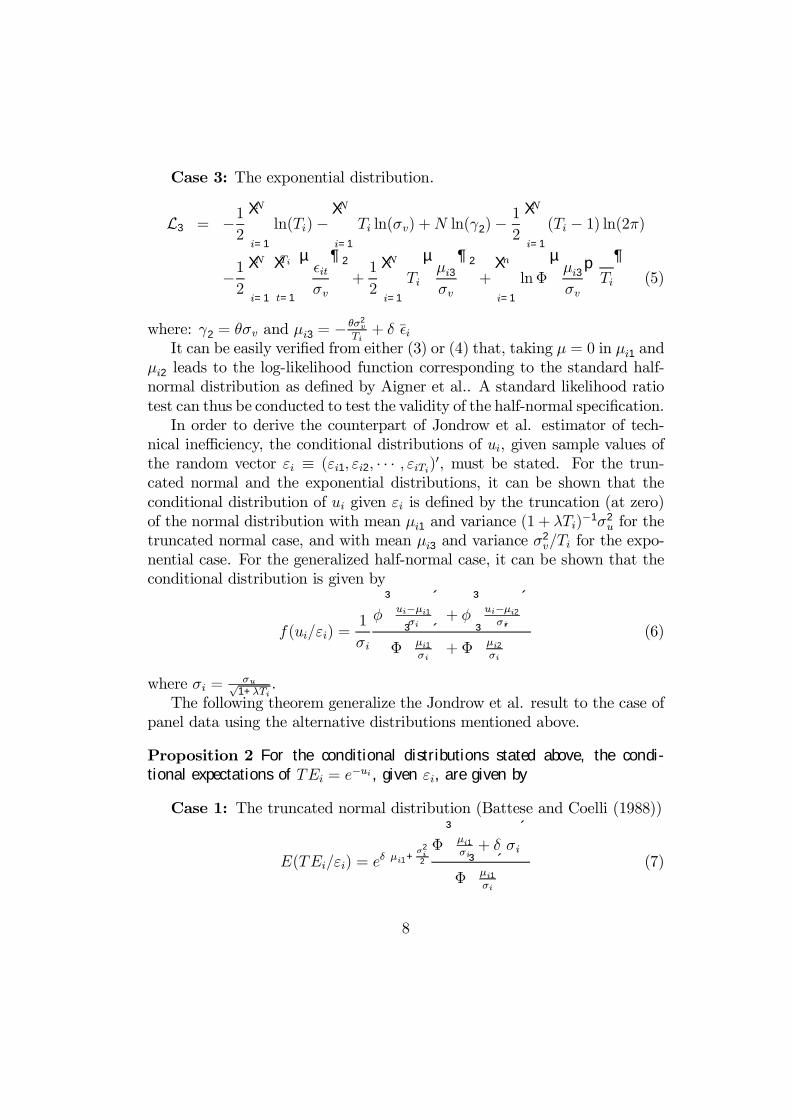
Case 3: The exponential distribution.

L3 = −12

NXi=1

ln(Ti)−NXi=1

Ti ln(σv) +N ln(γ2)−1

2

NXi=1

(Ti − 1) ln(2π)

−12

NXi=1

TiXt=1

µ²itσv

¶2

+1

2

NXi=1

Ti

µµi3σv

¶2

+nXi=1

lnΦ

µµi3σv

pTi

¶(5)

where: γ2 = θσv and µi3 = − θσ2v

Ti+ δ ²̄i

It can be easily veriÞed from either (3) or (4) that, taking µ = 0 in µi1 andµi2 leads to the log-likelihood function corresponding to the standard half-normal distribution as deÞned by Aigner et al.. A standard likelihood ratiotest can thus be conducted to test the validity of the half-normal speciÞcation.In order to derive the counterpart of Jondrow et al. estimator of tech-

nical inefficiency, the conditional distributions of ui, given sample values ofthe random vector εi ≡ (εi1, εi2, · · · , εiTi)0, must be stated. For the trun-cated normal and the exponential distributions, it can be shown that theconditional distribution of ui given εi is deÞned by the truncation (at zero)of the normal distribution with mean µi1 and variance (1 + λTi)

−1σ2u for the

truncated normal case, and with mean µi3 and variance σ2v/Ti for the expo-

nential case. For the generalized half-normal case, it can be shown that theconditional distribution is given by

f (ui/εi) =1

σi

φ³ui−µi1σi

´+ φ

³ui−µi2σi

´Φ

³µi1σi

´+ Φ

³µi2σi

´ (6)

where σi = σu√1+λTi

.The following theorem generalize the Jondrow et al. result to the case of

panel data using the alternative distributions mentioned above.

Proposition 2 For the conditional distributions stated above, the condi-tional expectations of TEi = e−ui , given εi, are given by

Case 1: The truncated normal distribution (Battese and Coelli (1988))

E(TEi/εi) = eδ µi1+

σ2i

2

Φ³µi1σi+ δ σi

´Φ

³µi1σi

´ (7)

8

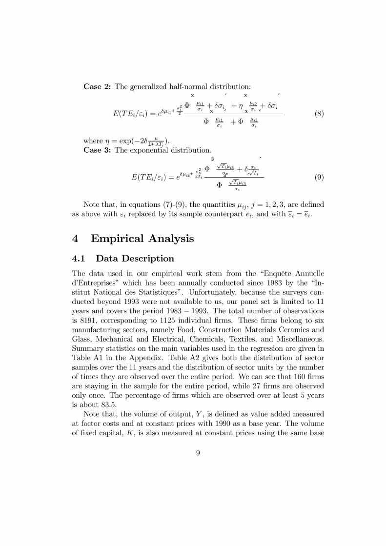
Case 2: The generalized half-normal distribution:

E(TEi/εi) = eδµi1+

σ2i

2

Φ³µi1σi+ δσi

´+ η

³µi2σi+ δσi

´Φ

³µi1σi

´+ Φ

³µi2σi

´ (8)

where η = exp(−2δ µ1+λTi

).Case 3: The exponential distribution.

E(TEi/εi) = eδµi3+

σ2v

2Ti

Φ³√

Tiµi3σv

+ δ σv√Ti

´Φ

³√Tiµi3σv

´ (9)

Note that, in equations (7)-(9), the quantities µij, j = 1, 2, 3, are deÞnedas above with εi replaced by its sample counterpart ei, and with εi = ei.

4 Empirical Analysis

4.1 Data Description

The data used in our empirical work stem from the �Enquête Annuelled�Entreprises� which has been annually conducted since 1983 by the �In-stitut National des Statistiques�. Unfortunately, because the surveys con-ducted beyond 1993 were not available to us, our panel set is limited to 11years and covers the period 1983 − 1993. The total number of observationsis 8191, corresponding to 1125 individual Þrms. These Þrms belong to sixmanufacturing sectors, namely Food, Construction Materials Ceramics andGlass, Mechanical and Electrical, Chemicals, Textiles, and Miscellaneous.Summary statistics on the main variables used in the regression are given inTable A1 in the Appendix. Table A2 gives both the distribution of sectorsamples over the 11 years and the distribution of sector units by the numberof times they are observed over the entire period. We can see that 160 Þrmsare staying in the sample for the entire period, while 27 Þrms are observedonly once. The percentage of Þrms which are observed over at least 5 yearsis about 83.5.Note that, the volume of output, Y , is deÞned as value added measured

at factor costs and at constant prices with 1990 as a base year. The volumeof Þxed capital, K, is also measured at constant prices using the same base

9

year. Labor, L, is deÞned as total employment and is measured by thenumber of employees. And Þnally, the capital vintage, agek, is measured asthe average age of equipments. A detailed information on the procedure usedto construct these variables may be found in Zribi (1995).

4.2 Frontier SpeciÞcation

The production technology is assumed to be described by the transcendentallogarithmic form, T-L, suggested by Christensen et al. (1973), which pro-vides a second-order Taylor-series approximation to any twice-differentiableproduction function. The advantage of this ßexible speciÞcation is twofold.Firstly, it allows the elasticities of output to vary across Þrms and acrossperiods. Secondly, it allows to test, through exclusion restrictions on someparameters, the empirical plausibility of the restrictive Cobb-Douglas, C-D,speciÞcation. Formally the model we estimate can be written as

yit = α + γ1t+ γ2t2 + (βk + γkt)kit + (β l + γlt)lit + (βa + γat)agekit

+0.5βkkk2 + βkl(kit × lit) + βka(kit × agekit) + 0.5βlll2it (10)

+β la(lit × agekit) + 0.5βaaagek2it + δfoodS1 + δcmcgS2 + δchimS4

+δtextS5 + δMiscS6 + vit − uiwhere y, k and l, denote, respectively, logarithms of Y , K and L. Thetime variable t is included as a regressor in order to catch neutral technicalprogress in production7. This implies that some of the shifts in the produc-tion frontier are allowed to occur independently of changes in inputs. Thedummy variables Si are introduced in order to take into account some secto-rial heterogeneity, and their effects must be interpreted in comparison withthe omitted Mechanical and Electrical sector.

4.3 Empirical Results

In this section, the translog frontier model deÞned by (10) is estimated, alongwith the Cobb-Douglas frontier, by maximum likelihood method using alter-native distributions for the one-sided error term8. These distributions are

7See Solow (1957).8The use of the ML method supposes that the speciÞc effects is random rather than

Þxed. This is the case here since the Hausman test statistic equals 199.42 which is largelygreater than the χ214 critical value.

10

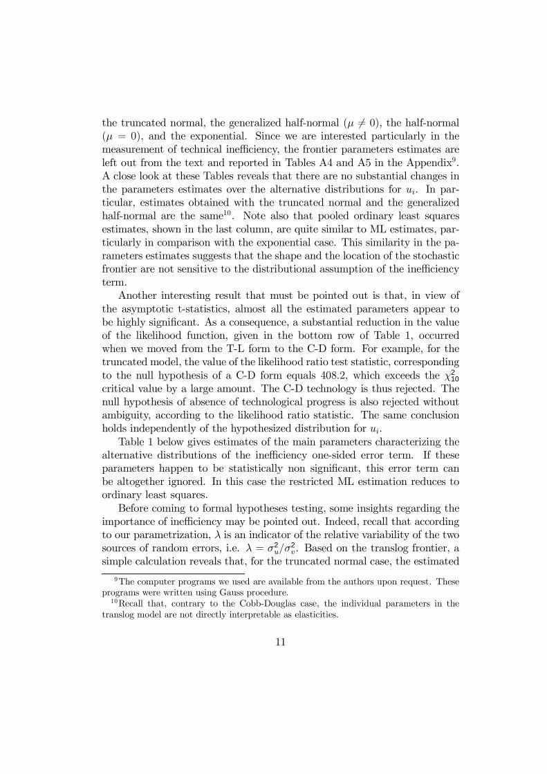
the truncated normal, the generalized half-normal (µ 6= 0), the half-normal(µ = 0), and the exponential. Since we are interested particularly in themeasurement of technical inefficiency, the frontier parameters estimates areleft out from the text and reported in Tables A4 and A5 in the Appendix9.A close look at these Tables reveals that there are no substantial changes inthe parameters estimates over the alternative distributions for ui. In par-ticular, estimates obtained with the truncated normal and the generalizedhalf-normal are the same10. Note also that pooled ordinary least squaresestimates, shown in the last column, are quite similar to ML estimates, par-ticularly in comparison with the exponential case. This similarity in the pa-rameters estimates suggests that the shape and the location of the stochasticfrontier are not sensitive to the distributional assumption of the inefficiencyterm.Another interesting result that must be pointed out is that, in view of

the asymptotic t-statistics, almost all the estimated parameters appear tobe highly signiÞcant. As a consequence, a substantial reduction in the valueof the likelihood function, given in the bottom row of Table 1, occurredwhen we moved from the T-L form to the C-D form. For example, for thetruncated model, the value of the likelihood ratio test statistic, correspondingto the null hypothesis of a C-D form equals 408.2, which exceeds the χ2

10

critical value by a large amount. The C-D technology is thus rejected. Thenull hypothesis of absence of technological progress is also rejected withoutambiguity, according to the likelihood ratio statistic. The same conclusionholds independently of the hypothesized distribution for ui.Table 1 below gives estimates of the main parameters characterizing the

alternative distributions of the inefficiency one-sided error term. If theseparameters happen to be statistically non signiÞcant, this error term canbe altogether ignored. In this case the restricted ML estimation reduces toordinary least squares.Before coming to formal hypotheses testing, some insights regarding the

importance of inefficiency may be pointed out. Indeed, recall that accordingto our parametrization, λ is an indicator of the relative variability of the twosources of random errors, i.e. λ = σ2

u/σ2v. Based on the translog frontier, a

simple calculation reveals that, for the truncated normal case, the estimated

9The computer programs we used are available from the authors upon request. Theseprograms were written using Gauss procedure.10Recall that, contrary to the Cobb-Douglas case, the individual parameters in the

translog model are not directly interpretable as elasticities.

11

variance of ui is about 44.7 percent of the estimated entire disturbance vari-ance, V (ui) + σ2

v which is equal to 0.1211. The Þgure is very different for the

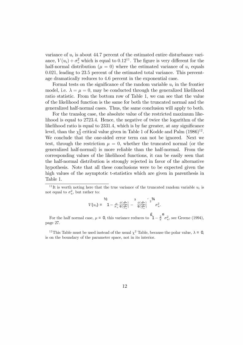
half-normal distribution (µ = 0) where the estimated variance of ui equals0.021, leading to 23.5 percent of the estimated total variance. This percent-age dramatically reduces to 4.6 percent in the exponential case.Formal tests on the signiÞcance of the random variable ui in the frontier

model, i.e. λ = µ = 0, may be conducted through the generalized likelihoodratio statistic. From the bottom row of Table 1, we can see that the valueof the likelihood function is the same for both the truncated normal and thegeneralized half-normal cases. Thus, the same conclusion will apply to both.For the translog case, the absolute value of the restricted maximum like-

lihood is equal to 2723.4. Hence, the negative of twice the logarithm of thelikelihood ratio is equal to 2331.4, which is by far greater, at any signiÞcancelevel, than the χ2

2 critical value given in Table 1 of Kodde and Palm (1986)12.

We conclude that the one-sided error term can not be ignored. Next wetest, through the restriction µ = 0, whether the truncated normal (or thegeneralized half-normal) is more reliable than the half-normal. From thecorresponding values of the likelihood functions, it can be easily seen thatthe half-normal distribution is strongly rejected in favor of the alternativehypothesis. Note that all these conclusions were to be expected given thehigh values of the asymptotic t-statistics which are given in parenthesis inTable 1.11It is worth noting here that the true variance of the truncated random variable ui is

not equal to σ2u, but rather to:

V (ui) =

½1− µ

σu

φ( µσu)

Φ( µσu)−

³φ( µ

σu)

Φ( µσu)

´2¾σ2u.

For the half normal case, µ = 0, this variance reduces to£1− 2

π

¤σ2u, see Greene (1994),

page 27.

12This Table must be used instead of the usual χ2 Table, because the polar value, λ = 0,is on the boundary of the parameter space, not in its interior.

12

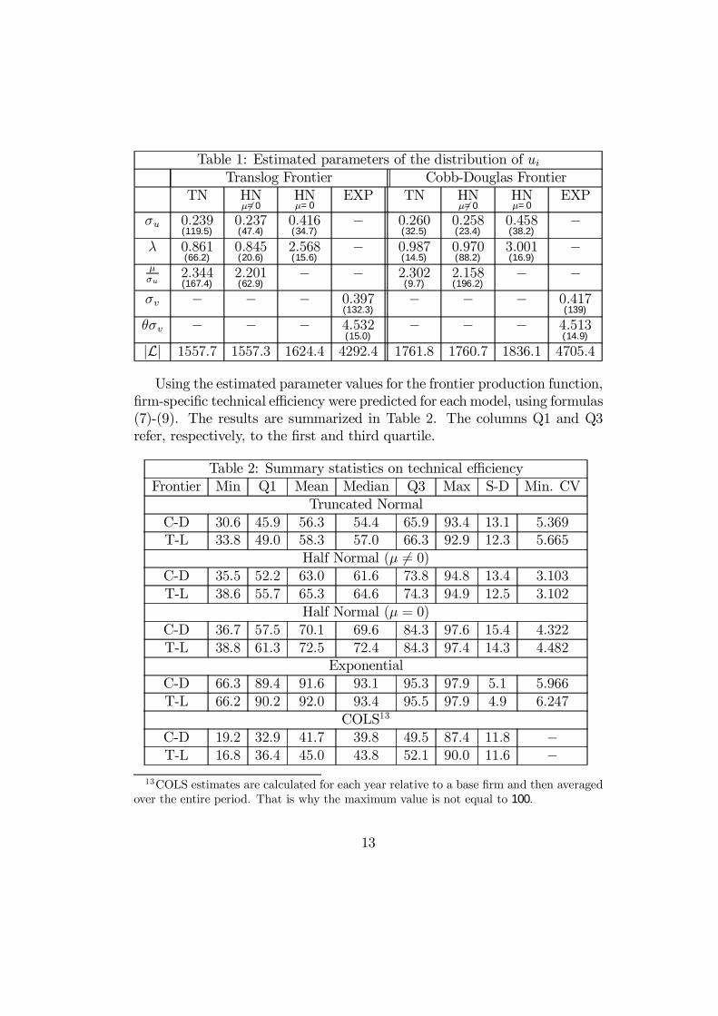
Table 1: Estimated parameters of the distribution of uiTranslog Frontier Cobb-Douglas Frontier

TN HNµ6=0

HNµ=0

EXP TN HNµ6=0

HNµ=0

EXP

σu 0.239(119.5)

0.237(47.4)

0.416(34.7)

− 0.260(32.5)

0.258(23.4)

0.458(38.2)

−λ 0.861

(66.2)0.845(20.6)

2.568(15.6)

− 0.987(14.5)

0.970(88.2)

3.001(16.9)

−µσu

2.344(167.4)

2.201(62.9)

− − 2.302(9.7)

2.158(196.2)

− −σv − − − 0.397

(132.3)− − − 0.417

(139)

θσv − − − 4.532(15.0)

− − − 4.513(14.9)

|L| 1557.7 1557.3 1624.4 4292.4 1761.8 1760.7 1836.1 4705.4

Using the estimated parameter values for the frontier production function,Þrm-speciÞc technical efficiency were predicted for each model, using formulas(7)-(9). The results are summarized in Table 2. The columns Q1 and Q3refer, respectively, to the Þrst and third quartile.

Table 2: Summary statistics on technical efficiencyFrontier Min Q1 Mean Median Q3 Max S-D Min. CV

Truncated NormalC-D 30.6 45.9 56.3 54.4 65.9 93.4 13.1 5.369T-L 33.8 49.0 58.3 57.0 66.3 92.9 12.3 5.665

Half Normal (µ 6= 0)C-D 35.5 52.2 63.0 61.6 73.8 94.8 13.4 3.103T-L 38.6 55.7 65.3 64.6 74.3 94.9 12.5 3.102

Half Normal (µ = 0)C-D 36.7 57.5 70.1 69.6 84.3 97.6 15.4 4.322T-L 38.8 61.3 72.5 72.4 84.3 97.4 14.3 4.482

ExponentialC-D 66.3 89.4 91.6 93.1 95.3 97.9 5.1 5.966T-L 66.2 90.2 92.0 93.4 95.5 97.9 4.9 6.247

COLS13

C-D 19.2 32.9 41.7 39.8 49.5 87.4 11.8 −T-L 16.8 36.4 45.0 43.8 52.1 90.0 11.6 −

13COLS estimates are calculated for each year relative to a base Þrm and then averagedover the entire period. That is why the maximum value is not equal to 100.

13

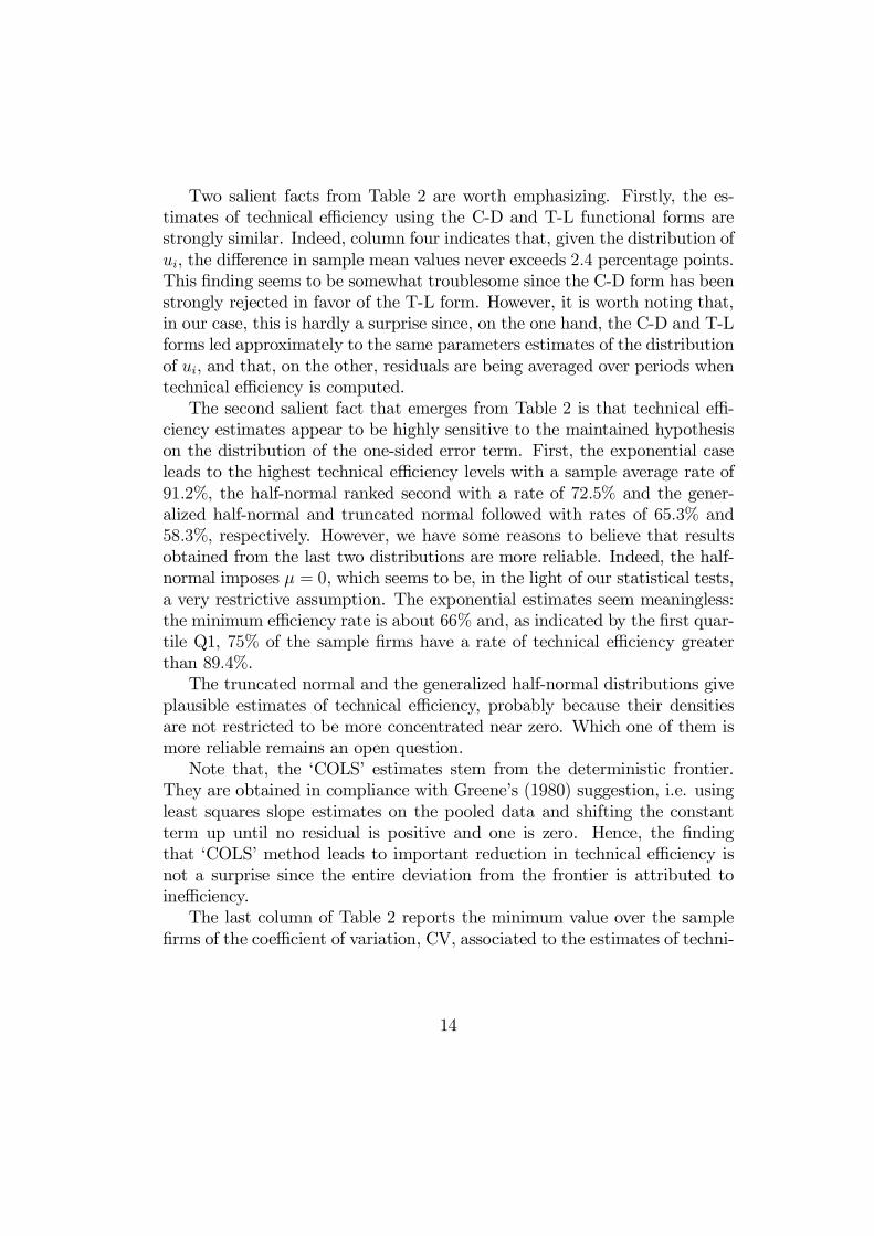
Two salient facts from Table 2 are worth emphasizing. Firstly, the es-timates of technical efficiency using the C-D and T-L functional forms arestrongly similar. Indeed, column four indicates that, given the distribution ofui, the difference in sample mean values never exceeds 2.4 percentage points.This Þnding seems to be somewhat troublesome since the C-D form has beenstrongly rejected in favor of the T-L form. However, it is worth noting that,in our case, this is hardly a surprise since, on the one hand, the C-D and T-Lforms led approximately to the same parameters estimates of the distributionof ui, and that, on the other, residuals are being averaged over periods whentechnical efficiency is computed.The second salient fact that emerges from Table 2 is that technical effi-

ciency estimates appear to be highly sensitive to the maintained hypothesison the distribution of the one-sided error term. First, the exponential caseleads to the highest technical efficiency levels with a sample average rate of91.2%, the half-normal ranked second with a rate of 72.5% and the gener-alized half-normal and truncated normal followed with rates of 65.3% and58.3%, respectively. However, we have some reasons to believe that resultsobtained from the last two distributions are more reliable. Indeed, the half-normal imposes µ = 0, which seems to be, in the light of our statistical tests,a very restrictive assumption. The exponential estimates seem meaningless:the minimum efficiency rate is about 66% and, as indicated by the Þrst quar-tile Q1, 75% of the sample Þrms have a rate of technical efficiency greaterthan 89.4%.The truncated normal and the generalized half-normal distributions give

plausible estimates of technical efficiency, probably because their densitiesare not restricted to be more concentrated near zero. Which one of them ismore reliable remains an open question.Note that, the �COLS� estimates stem from the deterministic frontier.

They are obtained in compliance with Greene�s (1980) suggestion, i.e. usingleast squares slope estimates on the pooled data and shifting the constantterm up until no residual is positive and one is zero. Hence, the Þndingthat �COLS� method leads to important reduction in technical efficiency isnot a surprise since the entire deviation from the frontier is attributed toinefficiency.The last column of Table 2 reports the minimum value over the sample

Þrms of the coefficient of variation, CV, associated to the estimates of techni-

14

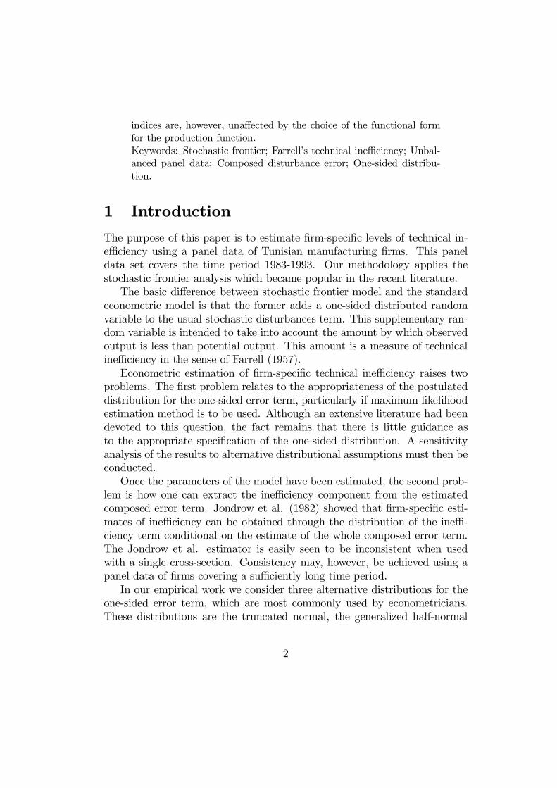
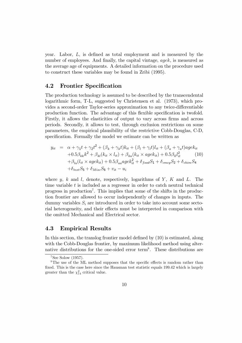
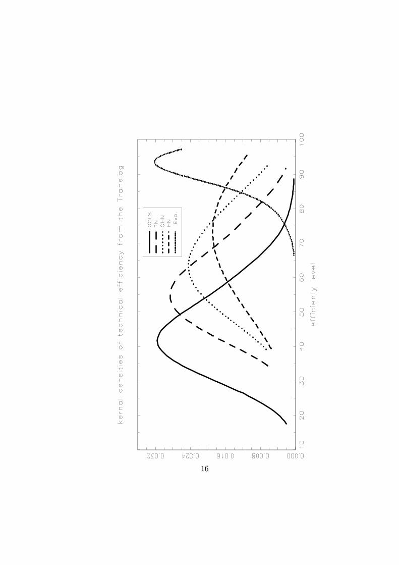
cal inefficiency14. It shows that all our estimates of efficiency are statisticallyquite accurate.The Þgure above illustrates the estimated kernal densities of the esti-

mated Þrm-technical efficiencies. It clearly reinforces our previous Þndingthat different assumptions about the distribution of ui leads to quite differ-ent measures of Þrm-technical efficiency. In particular, the expected upwardbias in the exponential case and the downward bias inherent to the deter-ministic case, i.e. COLS estimates, are apparent. The estimated densities forthe three other cases deviate substantially from each other, with as expectedthat corresponding to the half-normal assumption is to the right of those ofthe truncated normal and the generalized half-normal assumptions.

14CV is the coefficient of variation of the technical efficiency. Note that the variance oftechnical efficiency is easily calculated for a truncated normal X of mean µ and varianceσ2, using the following formula:

E(eaX) = exp(aµ+ .5a2 σ2)Φ(µσ+aσ)

Φ(µσ ).

This formula also applies, with a minor change, for the generalized half normal case.

15

16

5 Concluding remarksThis paper provides alternative measures of technical inefficiency dependingon what type of distributional assumptions for the one sided error term areconsidered. These assumptions include the most commonly used one-sideddistributions, namely the half-normal, the exponential and the truncatednormal distributions. A generalized version of the half-normal, which doesnot embody the zero-mean restriction, is also suggested.Comparisons of the estimated technical inefficiency indices induced by all

these distributions were attempted using a panel data on Tunisian manufac-turing Þrms over the 1983-1993 time period.Our main Þndings can be summarized as follows. Firstly, absence of tech-

nical inefficiency is wrongly rejected. This implies that the one-sided errorterm must be taken into account explicitly when econometric estimation offrontier function is in order. Secondly, estimates of technical efficiency seemto be insensitive to the degree of ßexibility of the frontier production func-tion. Indeed, the Cobb-Douglas technology gives almost the same estimatesof efficiency as the translog functional form. Thirdly, different assumptionson the distribution of technical inefficiency imply quite different estimates ofefficiency.The estimated inefficiencies suggest that the restricted models, i.e. the

exponential and, to a lesser degree, the half-normal, produce a very optimisticimpression, with an average rate of efficiency of 92% and 72.5%, respectively.It is worth noting, however, that formal test led to a strong rejection of thezero-mean half-normal model.Based on the truncated normal or the generalized half normal models, we

Þnd that Tunisian Þrms had been inefficient over the period 1983-1993; theaverage rate of inefficiency being approximately equal to 40%. Fifty percentof the sampled Þrms have a rate of efficiency between 58.3% and 66.3% for thetruncated normal case; the counterpart is 65.3 and 74.3% for the generalizedhalf normal case.

17

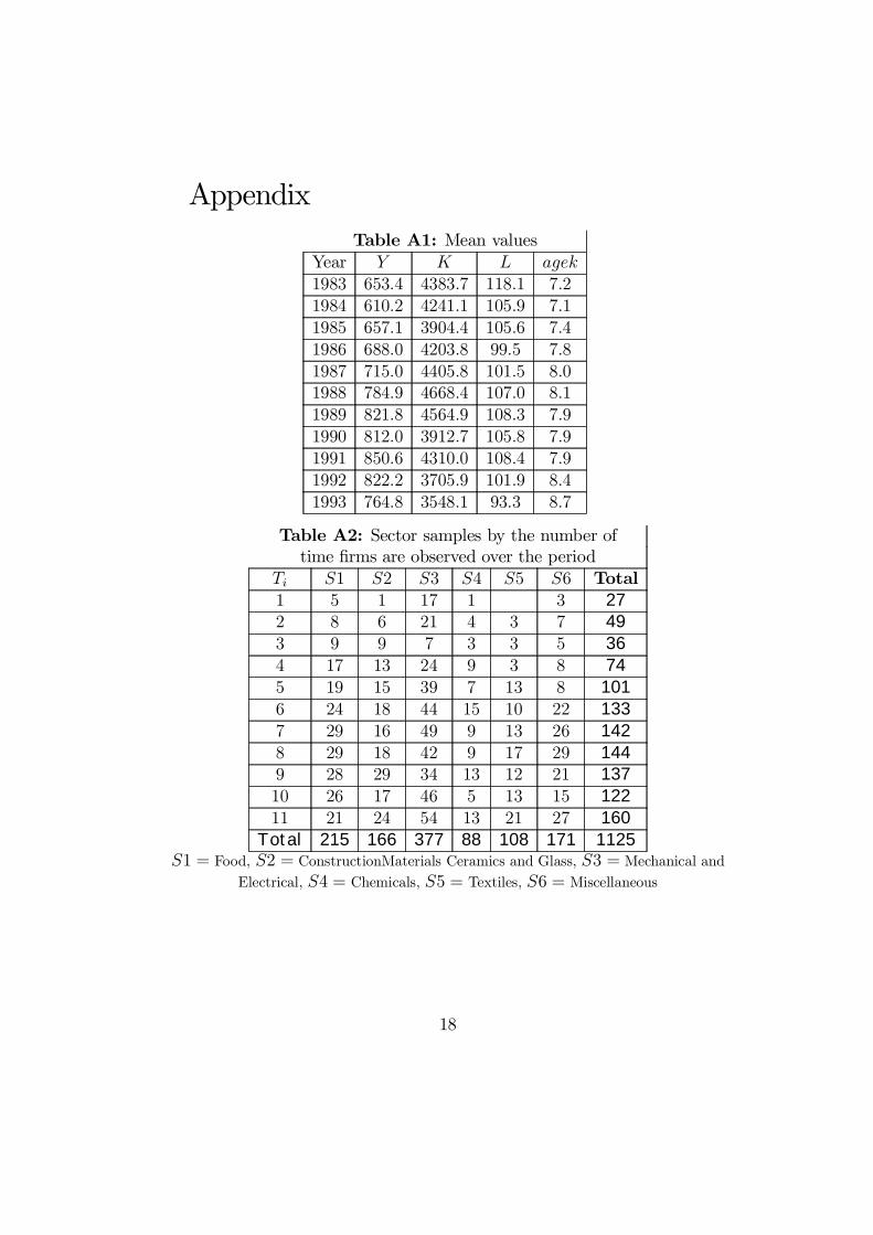
AppendixTable A1: Mean values

Year Y K L agek1983 653.4 4383.7 118.1 7.21984 610.2 4241.1 105.9 7.11985 657.1 3904.4 105.6 7.41986 688.0 4203.8 99.5 7.81987 715.0 4405.8 101.5 8.01988 784.9 4668.4 107.0 8.11989 821.8 4564.9 108.3 7.91990 812.0 3912.7 105.8 7.91991 850.6 4310.0 108.4 7.91992 822.2 3705.9 101.9 8.41993 764.8 3548.1 93.3 8.7

Table A2: Sector samples by the number oftime Þrms are observed over the period

Ti S1 S2 S3 S4 S5 S6 Total1 5 1 17 1 3 272 8 6 21 4 3 7 493 9 9 7 3 3 5 364 17 13 24 9 3 8 745 19 15 39 7 13 8 1016 24 18 44 15 10 22 1337 29 16 49 9 13 26 1428 29 18 42 9 17 29 1449 28 29 34 13 12 21 13710 26 17 46 5 13 15 12211 21 24 54 13 21 27 160

Total 215 166 377 88 108 171 1125S1 = Food, S2 = ConstructionMaterials Ceramics and Glass, S3 = Mechanical and

Electrical, S4 = Chemicals, S5 = Textiles, S6 = Miscellaneous

18

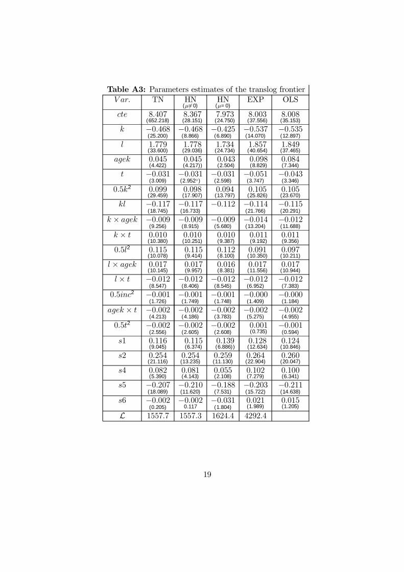
Table A3: Parameters estimates of the translog frontierV ar. TN HN

(µ6=0)HN

(µ=0)EXP OLS

cte 8.407(652.218)

8.367(28.151)

7.973(24.750)

8.003(37.556)

8.008(35.153)

k −0.468(25.200)

−0.468(8.866)

−0.425(6.890)

−0.537(14.070)

−0.535(12.897)

l 1.779(33.600)

1.778(29.036)

1.734(24.734)

1.857(40.654)

1.849(37.465)

agek 0.045(4.422)

0.045(4.217))

0.043(2.504)

0.098(8.829)

0.084(7.344)

t −0.031(3.009)

−0.031(2.952◦)

−0.031(2.598)

−0.051(3.747)

−0.043(3.346)

0.5k2 0.099(29.459)

0.098(17.907)

0.094(13.797)

0.105(25.826)

0.105(23.670)

kl −0.117(18.745)

−0.117(16.733)

−0.112 −0.114(21.766)

−0.115(20.291)

k × agek −0.009(9.256)

−0.009(8.915)

−0.009(5.680)

−0.014(13.204)

−0.012(11.688)

k × t 0.010(10.380)

0.010(10.251)

0.010(9.387)

0.011(9.192)

0.011(9.356)

0.5l2 0.115(10.078)

0.115(9.414)

0.112(8.100)

0.091(10.350)

0.097(10.211)

l × agek 0.017(10.145)

0.017(9.957)

0.016(8.381)

0.017(11.556)

0.017(10.944)

l× t −0.012(8.547)

−0.012(8.406)

−0.012(8.545)

−0.012(6.952)

−0.012(7.383)

0.5inc2 −0.001(1.726)

−0.001(1.749)

−0.001(1.748)

−0.000(1.409)

−0.000(1.184)

agek × t −0.002(4.213)

−0.002(4.186)

−0.002(3.783)

−0.002(5.275)

−0.002(4.955)

0.5t2 −0.002(2.556)

−0.002(2.605)

−0.002(2.608)

0.001(0.735)

−0.001(0.594)

s1 0.116(9.045)

0.115(6.374)

0.139(6.886))

0.128(12.634)

0.124(10.846)

s2 0.254(21.116)

0.254(13.235)

0.259(11.130)

0.264(22.904)

0.260(20.047)

s4 0.082(5.390)

0.081(4.143)

0.055(2.108)

0.102(7.279)

0.100(6.341)

s5 −0.207(18.089)

−0.210(11.620)

−0.188(7.531)

−0.203(15.722)

−0.211(14.638)

s6 −0.002(0.205)

−0.0020.117

−0.031(1.804)

0.021(1.989)

0.015(1.205)

L 1557.7 1557.3 1624.4 4292.4

19

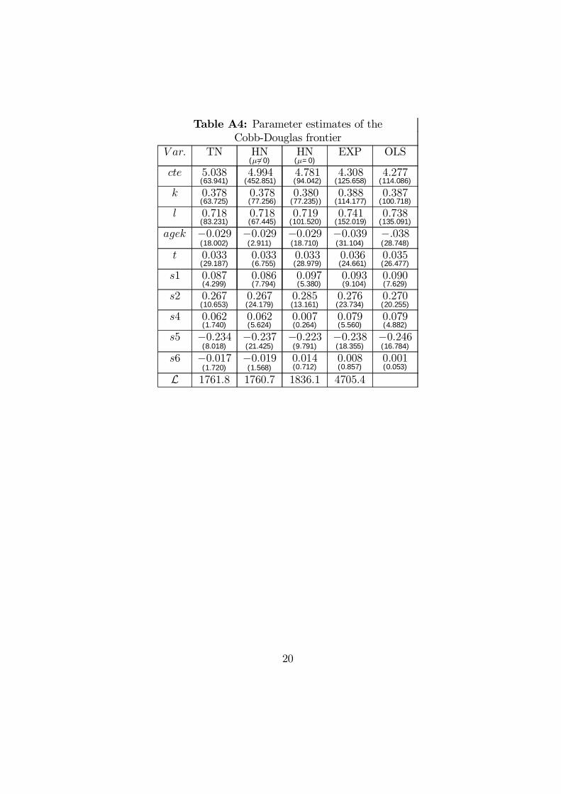
Table A4: Parameter estimates of theCobb-Douglas frontier

V ar. TN HN(µ6=0)

HN(µ=0)

EXP OLS

cte 5.038(63.941)

4.994(452.851)

4.781(94.042)

4.308(125.658)

4.277(114.086)

k 0.378(63.725)

0.378(77.256)

0.380(77.235))

0.388(114.177)

0.387(100.718)

l 0.718(83.231)

0.718(67.445)

0.719(101.520)

0.741(152.019)

0.738(135.091)

agek −0.029(18.002)

−0.029(2.911)

−0.029(18.710)

−0.039(31.104)

−.038(28.748)

t 0.033(29.187)

0.033(6.755)

0.033(28.979)

0.036(24.661)

0.035(26.477)

s1 0.087(4.299)

0.086(7.794)

0.097(5.380)

0.093(9.104)

0.090(7.629)

s2 0.267(10.653)

0.267(24.179)

0.285(13.161)

0.276(23.734)

0.270(20.255)

s4 0.062(1.740)

0.062(5.624)

0.007(0.264)

0.079(5.560)

0.079(4.882)

s5 −0.234(8.018)

−0.237(21.425)

−0.223(9.791)

−0.238(18.355)

−0.246(16.784)

s6 −0.017(1.720)

−0.019(1.568)

0.014(0.712)

0.008(0.857)

0.001(0.053)

L 1761.8 1760.7 1836.1 4705.4

20

References[1] Aigner, D.J., Lovell, C.A.K. and Schmidt,P. (1977), �Formulation and

Estimation of Stochastic Frontier Production Function Models�, Journalof Econometrics, 6, 21- 37.

[2] Aigner, D.J. and S. Chu (1968), �On estimating the Industry ProductionFunction�, American Economic Review, 55, PP. 826-839.

[3] Battese, G.E. and Coelli, T.J. (1988), �Prediction of Firm-Level Tech-nical Efficiencies With a Generalised Frontier Production Function andPanel Data�, Journal of Econometrics, 38, 387-399.

[4] Battese, G.E. and Coelli, T.J. (1992), �Frontier Production Functions,Technical Efficiency and Panel Data: With Application to Paddy Farm-ers in India�, Journal of Productivity Analysis, 3, 153-169.

[5] Battese, G.E. and Coelli, T.J. (1995), �A Model for Technical Ineffi-ciency Effects in a Stochastic Frontier Production Function for PanelData�, Empirical Economics, 20, 325-332.

[6] Battese, G.E., Coelli, T.J. and Colby, T.C. (1989), �Estimation of Fron-tier Production Functions and the Efficiencies of Indian Farms UsingPanel Data From ICRISAT�s Village Level Studies�, Journal of Quanti-tative Economics, 5, 327-348.

[7] Bauer, P.W. (1990), �Recent Developments in the Econometric Estima-tion of Frontiers�, Journal of Econometrics, 46, 39-56.

[8] Christensen, L.R., D.W. Jorgensen and L.J. Lau(1973),�TranscendentalLogarithmic Production Frontiers,� Review of Economics and Statistics,55, pp. 28-45.

[9] Cornwell C., P. Schmidt, and R.C. Sickles(1990), Production FrontiersWith Cross-Sectional and Time-Series Variations in Efficiency Levels,Journal of Econometrics 46.

[10] Farrell, M. (1957), �The Measurement of Productive Efficiency,� Journalof the Royal Statistical Society A, general 120, pt. 3, pp. 253-281.

21

[11] Forsund, F.R., Lovell, C.A.K. and Schmidt, P. (1980), �A Survey ofFrontier Production Functions and of their Relationship to EfficiencyMeasurement�, Journal of Econometrics, 13, 5-25.

[12] Greene, W.H. (1994), �Frontier Production Functions�, in Fried, H.O.,Lovell, C.A.K. and Schmidt, S.S.(Eds), The Handbook of AppliedEconometrics, North Holland, vol. II.

[13] Hausman , J., and W. Taylor(1981),�Panel Data and Unobservable In-dividual Effects�, Econometrica, 49, pp. 1377-1398.

[14] Jondrow, J.,. Lovell, C.A.K Materov, I.S. and Schmidt, P. (1982), �Onestimation of Technical Inefficiency in the Stochastic Frontier Produc-tion Function Model�, Journal of Econometrics, 19, 233-238.

[15] Kalirajan, K., and J. Flinn(1983)�The Measurement of Farm SpeciÞcTechnical Efficiency�, Pakistan Journal of Applied Economics, 2, pp.167-180.

[16] Kumbhakar S.C.(1990), Production Frontiers, Panel Data, and TimeVarying technical inefficiency, Journal of Econometrics 46.

[17] Kodde David A. and Franz C. Palm (1986),�Wald Criteria for JointlyTesting Equality and Inequality Restrictions,� Econometrica, 54, 1243-1248.

[18] Lee, L.,(1993), �A Test for Distributional Assumptions for a StochasticFrontier Function�, Journal of Econometrics, 22, pp. 245-267.

[19] Meeusen, W. and van den Broeck, J. (1977), �Efficiency Estimation fromCobb- Douglas Production Functions With Composed Error�, Interna-tional Economic Review, 18, 435-444.

[20] Schmidt, P. (1986), �Frontier Production Functions�, Econometric Re-views, 4, 289- 328.

[21] Schmidt, P. and Lovell, C.A.K. (1980), �Estimating Technical and Al-locative Inefficiency Relative to Stochastic Production and Cost Fron-tiers�, Journal of Econometrics 13, 83-100.

[22] Schmidt, P. and R.C. Sickles(1984), Production Frontiers and PanelData, Journal of Business and Economic Statistics 2, 367-374.

22

[23] Solow, R. (1957),�Technical Change and the Aggregate ProductionFunction�, Reviw of Economics and Statistics, 39, 312-320.

[24] Stevenson, R.E. (1980), �Likelihood Functions for Generalised Stochas-tic Frontier Estimation�, Journal of Econometrics, 13, 57- 66.

[25] Zelner A., J. Kmenta and J. Drèze(1966),�SpeciÞcation and Estimationof Cobb-Douglas Production Models,� Econometrica, 34, pp. 784-795.

[26] Zribi Y. (1995), �La dynamique du capital Þxe productif des entreprisestunisiennes�, mimeo IEQ, N. 02-95.

23