Why Have Greenhouse Emissions in RGGI States Declined? An

Division of Economics and BusinessWorking Paper Series

Why Have Greenhouse Emissions in RGGI StatesDeclined? An Econometric Attribution to Economic,

Energy Market and Policy Factors

Brian C. MurrayPeter T. ManiloffEvan M. Murray

Working Paper 2014-04http://econbus.mines.edu/working-papers/wp201404.pdf

Colorado School of MinesDivision of Economics and Business

1500 Illinois StreetGolden, CO 80401

April 2014

c© 2014 by the listed authors. All rights reserved.

Colorado School of MinesDivision of Economics and BusinessWorking Paper No. 2014-04April 2014

Title:Why Have Greenhouse Emissions in RGGI States Declined? An Econometric Attribution toEconomic, Energy Market and Policy Factors∗

Author(s):Brian C. MurrayDuke University

Peter T. ManiloffDivision of Economics and BusinessColorado School of MinesGolden, CO [email protected]

Evan M. MurrayDuke University

ABSTRACT

The Regional Greenhouse Gas Initiative (RGGI) is a consortium of northeastern states that have agreed

to limit carbon dioxide emissions from electricity generation through a regional emissions trading program.

Since the initiative came into effect in 2009, emissions have dropped precipitously, while the price of emissions

allowances has fallen from approximately $4 per ton to the program floor price of just under $2.00. We ask

why the emission reductions have come so fast and inexpensively, finding that it is due to a combination

of factors, including the emissions trading program itself, complementary environmental programs, lower

natural gas prices, and possibly some regional spillover effects. We find that the effect of the recession was

small compared with other factors. Lower natural gas prices had a substantial impact on regional emissions.

Econometric challenges makes it difficult to assign how much of the RGGI reduction is due to the price

and how much is due to an overall “regime effect” guiding long-term planning decisions. We also present

results consistent with but not dispositive of RGGI emissions reductions being due to policy leakage. But

taken together, and compared to emission reduction outcomes in the rest of the U.S., it appears the RGGI

program has induced a substantial reduction in the emissions, all else equal.

∗The authors acknowledge comments on earlier drafts from Harrison Fell (Colorado School of Mine and RFF), Joe Aldy

(Harvard), Billy Pizer (Duke) and attendees at the 2013 AERE summer conference in Banff, Alberta. We also thank Karen

Palmer (RFF) for data used in a preliminary analysis of this work.

2

1. Introduction

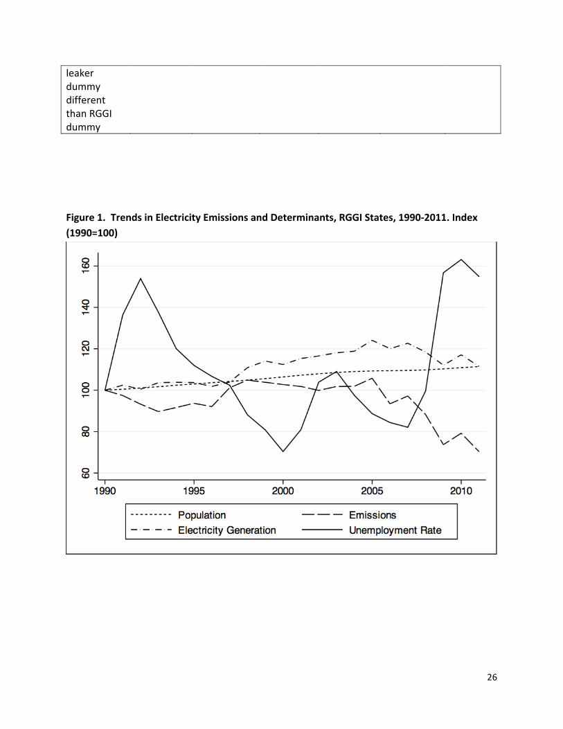
The Regional Greenhouse Gas Initiative (RGGI) is a consortium of northeastern U.S. states which have agreed to limit the greenhouse gas (GHG) emissions of carbon dioxide (CO2) from electric power generation via a regional emissions trading (“cap-‐and-‐trade”) program.1 Since RGGI came into effect in mid-‐2008, total emissions from the region’s power sector have plummeted substantially. Figure 1 depicts an index from 1990 to 2010 showing change in income, population, electricity generation and electricity emissions in RGGI states between 1990 and 2010.2 The figure outlines the percent change of a certain factor indexed to its value in 1990.

The most stark observation from these data is the sharp decline in electricity emissions in the later years. In 2005, the emissions were about equal to those of 1990, but by 2009, those emissions had fallen by around 30%. What is particularly interesting about that time period is that states started announcing their intentions to join RGGI in the middle of the decade, but the program did not commence until 2009, a point we will return to below.

Meanwhile, electricity generation stayed about the same after 2005, and had risen significantly since 1990. This widening gap between emissions and generation suggests a decarbonization of power generation as it transitions from coal and oil which emit much larger amounts per BTU of energy produced to lower or zero emitting fuel sources, such as natural gas, nuclear power and renewables, respectively. The shapes of the electricity generation and emissions functions are similar, usually increasing and decreasing in the same years as one another. They also share similar patterns of variation -‐ as generation increases, emissions increase similarly. Current emissions are not only well below historic levels, they are below the emissions cap that was established by the program. These retired allowances equaled over one-‐fifth of the legislated emissions cap for that period. As detailed further below, the allowances were unsold because of the existence of a price floor for RGGI auctions, below which no auction bids can be accepted.

Taken together, this suggests a system that has either been extremely effective, less stringent than it should be, overtaken by other economic, technological and market factors that are driving emissions down, or some combination of the above (LeGrand, 2013). The situation that 1 From 2009-‐2011, the 10 RGGI states were Connecticut, Delaware, Maine, Maryland, Massachusetts, New Hampshire, New Jersey, New York, Rhode Island, and Vermont. In 2012, New Jersey left the program. 2 Emissions and generation data are from the EIA data. Population estimates are from the BEA. Statewide unemployment rates are from the BLS. The population-‐weighted average presented here is the authors’ calculation.

3

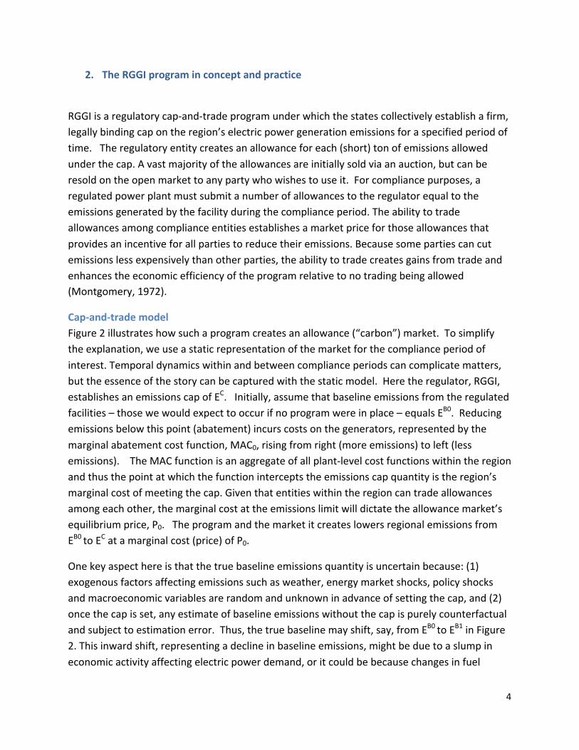
emerged in RGGI states after program inception suggests four possible factors driving the dramatic decline in emissions (Tietenberg, 2013; Stavins, 2012; Hibbard et al, 2011, Environment Northeast, 2011):

• The RGGI program itself, which sends a price signal to power generators favoring lower emitting sources and generates auction revenues to finance low carbon and energy efficiency investments within the region;

• The economic crisis commencing in 2008 and continuing for several years, which lowered economic activity, energy demand and emissions there from;

• The surge in the availability of lower-‐emitting natural gas due in part in to rapid expansion of hydraulic fracturing (“fracking”) technology; and

• Complementary state environmental programs such as renewable portfolio standards that mandate a certain share of electric power be generated by renewable (low or zero-‐emitting) sources.

This paper attempts to quantitatively decompose the emission reductions in the RGGI region into these and other factors. We do so by developing an econometric model of the U.S. electric power sector, including final demand for electricity, factor demand for alternative generation sources, and CO2 emissions. We use panel data from each of the 48 states in the continental U.S. for the time period 1991-‐2011 to estimate the model. This allows us to differentiate responses within the RGGI region and time frame from the rest of the population. The estimated model is then used to simulate the energy and emissions effects of counterfactual scenarios to quantify the separate effects of the RGGI program, macroeconomic factors, natural gas price shifts and other environmental policies.

The paper continues with a conceptual model that defines how the RGGI program works and how the cap-‐and-‐trade structure along with other factors influence emissions and price outcomes. The conceptual model informs a discussion the actual RGGI program allowance auction price and quantity outcomes since the inception of the program. The paper then discusses how various factors other than the RGGI program itself could have influenced emissions outcomes in the region. An econometric model of the power sector is used to estimate power demand, allocation of generation sources, and emissions with state-‐level time series data from 1990-‐2011. The estimated model is used to simulate counterfactual scenarios to quantitatively attribute emissions effects to policy and market factors. The paper concludes with a summary of key findings, caveats and recommendations for future work.

4

2. The RGGI program in concept and practice

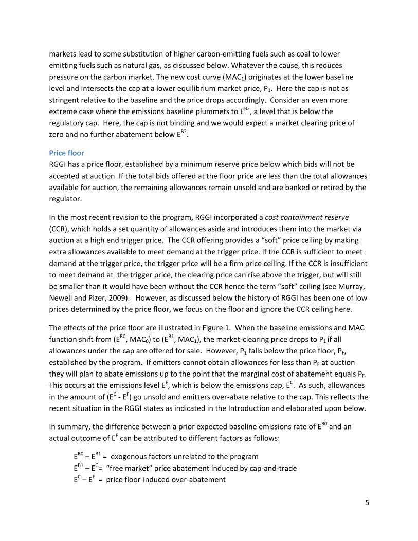
RGGI is a regulatory cap-‐and-‐trade program under which the states collectively establish a firm, legally binding cap on the region’s electric power generation emissions for a specified period of time. The regulatory entity creates an allowance for each (short) ton of emissions allowed under the cap. A vast majority of the allowances are initially sold via an auction, but can be resold on the open market to any party who wishes to use it. For compliance purposes, a regulated power plant must submit a number of allowances to the regulator equal to the emissions generated by the facility during the compliance period. The ability to trade allowances among compliance entities establishes a market price for those allowances that provides an incentive for all parties to reduce their emissions. Because some parties can cut emissions less expensively than other parties, the ability to trade creates gains from trade and enhances the economic efficiency of the program relative to no trading being allowed (Montgomery, 1972).

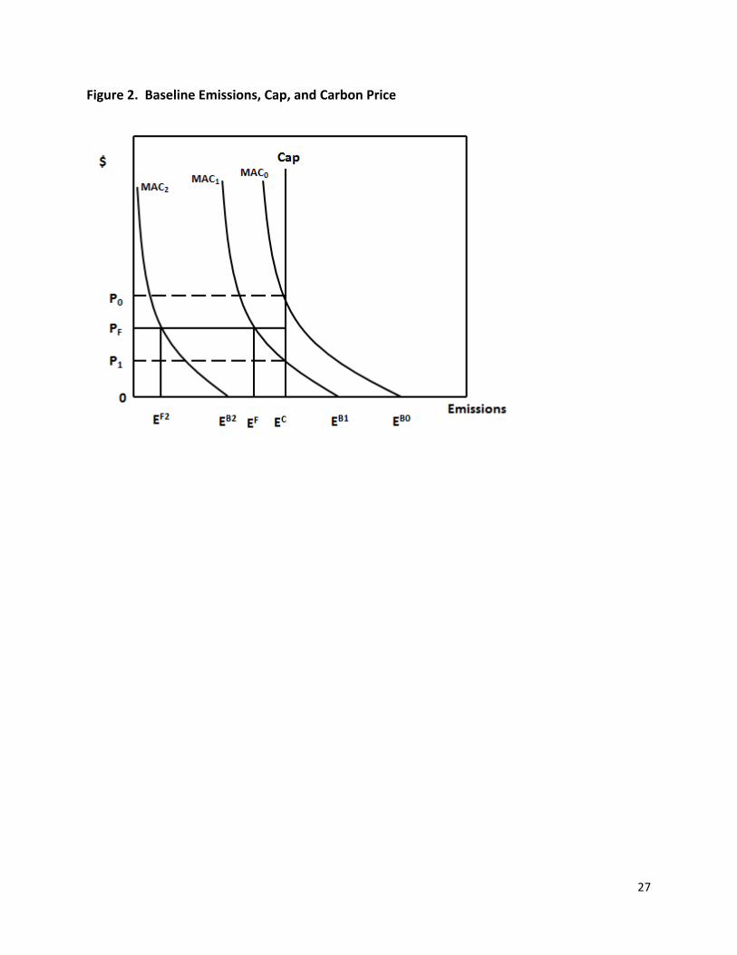
Cap-‐and-‐trade model Figure 2 illustrates how such a program creates an allowance (“carbon”) market. To simplify the explanation, we use a static representation of the market for the compliance period of interest. Temporal dynamics within and between compliance periods can complicate matters, but the essence of the story can be captured with the static model. Here the regulator, RGGI, establishes an emissions cap of EC. Initially, assume that baseline emissions from the regulated facilities – those we would expect to occur if no program were in place – equals EB0. Reducing emissions below this point (abatement) incurs costs on the generators, represented by the marginal abatement cost function, MAC0, rising from right (more emissions) to left (less emissions). The MAC function is an aggregate of all plant-‐level cost functions within the region and thus the point at which the function intercepts the emissions cap quantity is the region’s marginal cost of meeting the cap. Given that entities within the region can trade allowances among each other, the marginal cost at the emissions limit will dictate the allowance market’s equilibrium price, P0. The program and the market it creates lowers regional emissions from EB0 to EC at a marginal cost (price) of P0.

One key aspect here is that the true baseline emissions quantity is uncertain because: (1) exogenous factors affecting emissions such as weather, energy market shocks, policy shocks and macroeconomic variables are random and unknown in advance of setting the cap, and (2) once the cap is set, any estimate of baseline emissions without the cap is purely counterfactual and subject to estimation error. Thus, the true baseline may shift, say, from EB0 to EB1 in Figure 2. This inward shift, representing a decline in baseline emissions, might be due to a slump in economic activity affecting electric power demand, or it could be because changes in fuel

5

markets lead to some substitution of higher carbon-‐emitting fuels such as coal to lower emitting fuels such as natural gas, as discussed below. Whatever the cause, this reduces pressure on the carbon market. The new cost curve (MAC1) originates at the lower baseline level and intersects the cap at a lower equilibrium market price, P1. Here the cap is not as stringent relative to the baseline and the price drops accordingly. Consider an even more extreme case where the emissions baseline plummets to EB2, a level that is below the regulatory cap. Here, the cap is not binding and we would expect a market clearing price of zero and no further abatement below EB2.

Price floor RGGI has a price floor, established by a minimum reserve price below which bids will not be accepted at auction. If the total bids offered at the floor price are less than the total allowances available for auction, the remaining allowances remain unsold and are banked or retired by the regulator.

In the most recent revision to the program, RGGI incorporated a cost containment reserve (CCR), which holds a set quantity of allowances aside and introduces them into the market via auction at a high end trigger price. The CCR offering provides a “soft” price ceiling by making extra allowances available to meet demand at the trigger price. If the CCR is sufficient to meet demand at the trigger price, the trigger price will be a firm price ceiling. If the CCR is insufficient to meet demand at the trigger price, the clearing price can rise above the trigger, but will still be smaller than it would have been without the CCR hence the term “soft” ceiling (see Murray, Newell and Pizer, 2009). However, as discussed below the history of RGGI has been one of low prices determined by the price floor, we focus on the floor and ignore the CCR ceiling here.

The effects of the price floor are illustrated in Figure 1. When the baseline emissions and MAC function shift from (EB0, MAC0) to (EB1, MAC1), the market-‐clearing price drops to P1 if all allowances under the cap are offered for sale. However, P1 falls below the price floor, PF, established by the program. If emitters cannot obtain allowances for less than PF at auction they will plan to abate emissions up to the point that the marginal cost of abatement equals PF. This occurs at the emissions level EF, which is below the emissions cap, EC. As such, allowances in the amount of (EC -‐ EF) go unsold and emitters over-‐abate relative to the cap. This reflects the recent situation in the RGGI states as indicated in the Introduction and elaborated upon below.

In summary, the difference between a prior expected baseline emissions rate of EB0 and an actual outcome of EF can be attributed to different factors as follows:

EB0 – EB1 = exogenous factors unrelated to the program EB1 – EC = “free market” price abatement induced by cap-‐and-‐trade EC – EF = price floor-‐induced over-‐abatement

6

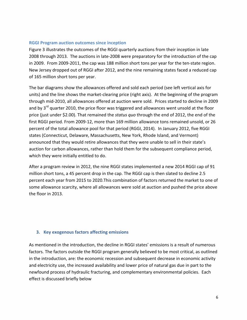
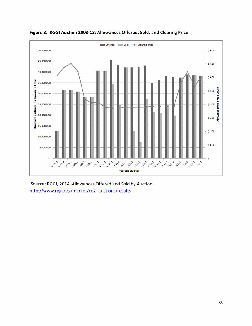
RGGI Program auction outcomes since inception Figure 3 illustrates the outcomes of the RGGI quarterly auctions from their inception in late 2008 through 2013. The auctions in late-‐2008 were preparatory for the introduction of the cap in 2009. From 2009-‐2011, the cap was 188 million short tons per year for the ten-‐state region. New Jersey dropped out of RGGI after 2012, and the nine remaining states faced a reduced cap of 165 million short tons per year.

The bar diagrams show the allowances offered and sold each period (see left vertical axis for units) and the line shows the market-‐clearing price (right axis). At the beginning of the program through mid-‐2010, all allowances offered at auction were sold. Prices started to decline in 2009 and by 3rd quarter 2010, the price floor was triggered and allowances went unsold at the floor price (just under $2.00). That remained the status quo through the end of 2012, the end of the first RGGI period. From 2009-‐12, more than 169 million allowance tons remained unsold, or 26 percent of the total allowance pool for that period (RGGI, 2014). In January 2012, five RGGI states (Connecticut, Delaware, Massachusetts, New York, Rhode Island, and Vermont) announced that they would retire allowances that they were unable to sell in their state’s auction for carbon allowances, rather than hold them for the subsequent compliance period, which they were initially entitled to do.

After a program review in 2012, the nine RGGI states implemented a new 2014 RGGI cap of 91 million short tons, a 45 percent drop in the cap. The RGGI cap is then slated to decline 2.5 percent each year from 2015 to 2020.This combination of factors returned the market to one of some allowance scarcity, where all allowances were sold at auction and pushed the price above the floor in 2013.

3. Key exogenous factors affecting emissions As mentioned in the introduction, the decline in RGGI states’ emissions is a result of numerous factors. The factors outside the RGGI program generally believed to be most critical, as outlined in the introduction, are: the economic recession and subsequent decrease in economic activity and electricity use, the increased availability and lower price of natural gas due in part to the newfound process of hydraulic fracturing, and complementary environmental policies. Each effect is discussed briefly below

7

The post-‐2008 recession The economic recession that gripped the region, country and most of the world may have played a role in driving down electricity generation. Reduced economic activity leads to a decline in energy use, resulting in fewer emissions and decreased demand for carbon allowances in the system. From 2008 to 2009, both GDP and total emissions declined for the first time since 1990 (Figure 1). GDP and total emissions follow a similar trend in growth, albeit emissions have risen at a much slower rate than GDP in the past 20 years. Moreover, emissions continued to decline even after economic activity started to pick up after the recession.

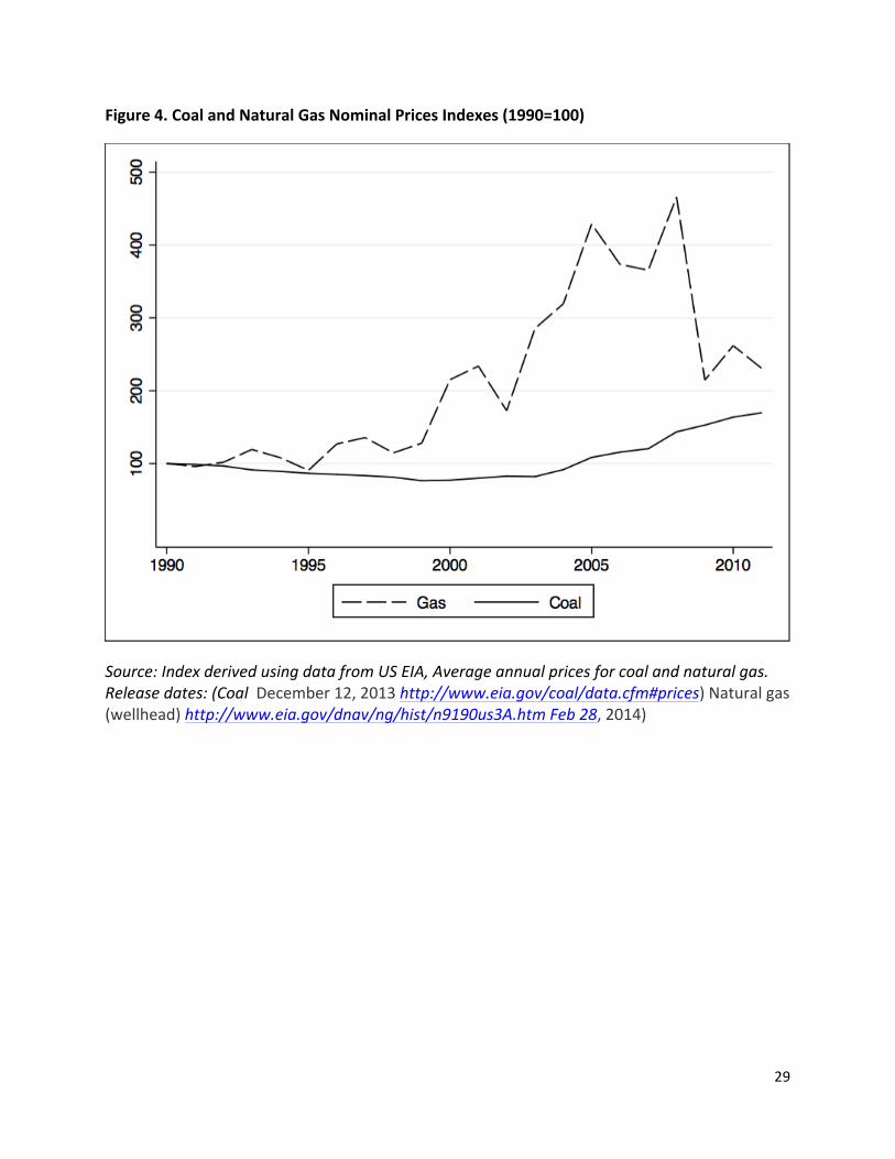
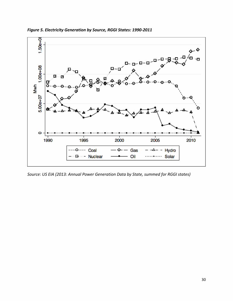
New natural gas discoveries Natural gas is the lowest GHG emitting fossil fuel, producing about 47% of the carbon dioxide per energy unit of coal (Moomaw et al, 2011). In its 2008 biennial assessment of natural gas reserves in the United States, the Potential Gas Committee of the Colorado School of Mines reported a 40 percent increase in available gas reserves relative to its previous assessment in 2006 (Potential Gas Committee, 2009). This unprecedented growth can be tied to the discovery of shale gas fields that had been previously written off as inaccessible or not worth pursuing. Now that companies have developed the process of hydraulic fracturing (or “fracking”) -‐ a method that shoots a pressurized mixture of water, sand and chemicals through shale rock, creating fractures in the rock and releasing gas-‐ the estimated size of the United States’ natural gas reserves has greatly increased. This relatively sudden expansion of natural gas supply contributed to the price of natural gas plummeting 46% between 2005 and 2011, while the price of coal rose (see Figure 4). Together with the economic recession, a large supply of natural gas has kept the price of natural gas low over the past few years. The market has reacted to these low prices by increasing use as a share of total energy generation. In 1990, natural gas accounted for 12% of electricity generation in the ten RGGI states. By 2011, however, that number had increased to about 40%. Meanwhile, coal reduced its market share from 25% of total generation in 1990 to only 11% in 2011. This monumental shift from coal to natural gas generation within the region clearly has had a profound impact on the region’s GHG emissions; however, the extent to which this is driven by pure energy market forces, environmental policy, or some combination is one of the foci of our analysis below.

Complementary policies The exogenous shifts in emissions could also be due to policies that are complementary to the RGGI cap-‐and-‐trade program, such as renewable portfolio standards (RPS) which exist in all of

8

the 10 original RGGI states.3 An RPS requires a certain portion of state power come from renewable non-‐emitting sources and thereby creates the kind of baseline emission reduction and MAC curve shifts depicted in Figure 1. Additionally, the RGGI program itself has a number of complementary measures within it, apart from the cap itself, aimed at reducing emissions, such as the use of RGGI auction revenues for energy efficiency purposes (Hibbard et al, 2011). Federal Clean Air Act regulations for air pollutants such as SO2, NOx and mercury all impose regulatory requirements on coal-‐powered generation that favor substitution to viable alternatives such as natural gas, nuclear, and renewables.

4. Empirical Analysis

Relevant literature Some policy organizations release data on RGGI emissions and provide opinions on the causes of the emissions trends (e.g, Environment Northeast, 2011), but to our knowledge no research has been published that statistically estimates RGGI programmatic effects versus other effects on emission reductions.

One study with a similar ambition to estimate a cap-‐and-‐trade program’s effect on emissions was performed for the EU Emissions Trading Scheme (EU ETS) by Ellerman and Buchner (2008). They analyze emissions data prior to and after introduction of Phase I of the EU ETS from 2005-‐2007 to gauge how much of the observed decline in the region’s emissions could be attributed to the EU ETS program, how much as attributable to secular trends in emission determinants such as weather, energy markets and improvements in energy efficiency and emissions intensity. They use a mix of quantitative and qualitative analysis of emissions data to develop different proxies for the counterfactual emissions that would have occurred without the ETS and estimate the program dropped emissions from as much as 8 percent to as little as 0.5 percent across the continent. Our analysis departs from Ellerman and Buchner by using time series cross-‐sectional econometric methods to estimate emissions as a function of a range of policy, market and environmental variables, which allows us to estimate the size and significance of different factors contributing to the emissions decline before after the RGGI program takes effect.

A paper by Chevallier (2011) seeks to econometrically estimate the relationship between macroeconomic and energy market factors and EU ETS carbon prices using a Markov-‐Switching VAR model , finding strong links between the factors but Chevallier’s ambition was not to quantify emissions reduction attribution, as is ours here.

3 The RPS is voluntary in Vermont.

9

Empirical strategy

Our empirical strategy is to first develop a three-‐stage econometric model of electricity generation at the state level. We then use this econometric model to simulate baseline emissions based on observed data as well as a variety of counterfactual scenarios which remove particular policies or observed market shocks.

Data and Econometric model In the first stage, we estimate the demand for state-‐level electricity generation as a function

of own price and demand shifters such as potential energy macroeconomic variables, weather variables, and policy variables. The first stage is estimated as equation 1.

𝑐!" = 𝑋!"𝛽 + 𝜇! + 𝜀!" [1]

where c is the detrended electricity capacity utilization factor for state i in year t, X includes detrended electricity price, detrended unemployment rate, population-‐weighted heating and cooling degree days (measures of weather-‐induced heating and cooling demand), the level of the state RPS, and a dummy for whether the state is under the RGGI program. The RGGI program uses some of its auction revenues for energy efficiency expenditures within the region (Hilliard et al 2011) which could shift power demand. We do not observe these expenditures directly. Instead we assume they are homogenous across RGGI states and use the RGGI dummy variable to capture its effects on demand. A state-‐level fixed effect is captured by µi, while εit is an iid unobservable.

The second stage estimates derived power demand by generation fuel type, conditional on own and cross-‐ fuel prices as well as total generation. This is estimated as equation 2.

𝑓!!" = 𝑌!Θ+ 𝑍!"Γ+ 𝜈! + 𝛿!" [2]

where fijt is the detrended capacity utilization factor for generation using fossil fuel j in state i in year t. Fuel type j is one of [coal, natural gas, oil]. For coal and gas generation, Yt includes U.S. average coal prices and wellhead natural gas prices while Zit includes the state capacity utilization factor (cit above), state RPS requirement, the detrended annual average carbon price for RGGI states, and a dummy variable for RGGI states in the RGGI compliance period.4 A state-‐level fixed effect is captured by νi, while δit is an iid unobservable.

4 These may depart from the actual prices which generators face in a variety of ways. Coal generators often use long-‐term contracts with pre-‐specified prices as well as entering the spot market. Coal is primarily distributed by rail, so generators’ actual procurement prices in the spot market will reflect both spot prices and rail prices.

10

Due to its high marginal cost, oil generation is now used sparingly in most states and typically only when demand is too high to be met with other generation sources. For oil generation, Yt includes West Texas Intermediate oil prices and wellhead natural gas prices while Zit includes the same set of variables as for gas and coal plants.

The third stage estimates CO2 emissions as a function of generation from fossil fuels as in equation 3.

𝑚!" = 𝑉!"Κ+ 𝜉! + 𝜎!" [3]

where mit is the emissions from state i in year t and Vit includes generation from coal, gas, and oil generation in state i in year t. A state-‐level fixed effect is captured by ξi, while σit is an iid unobservable.

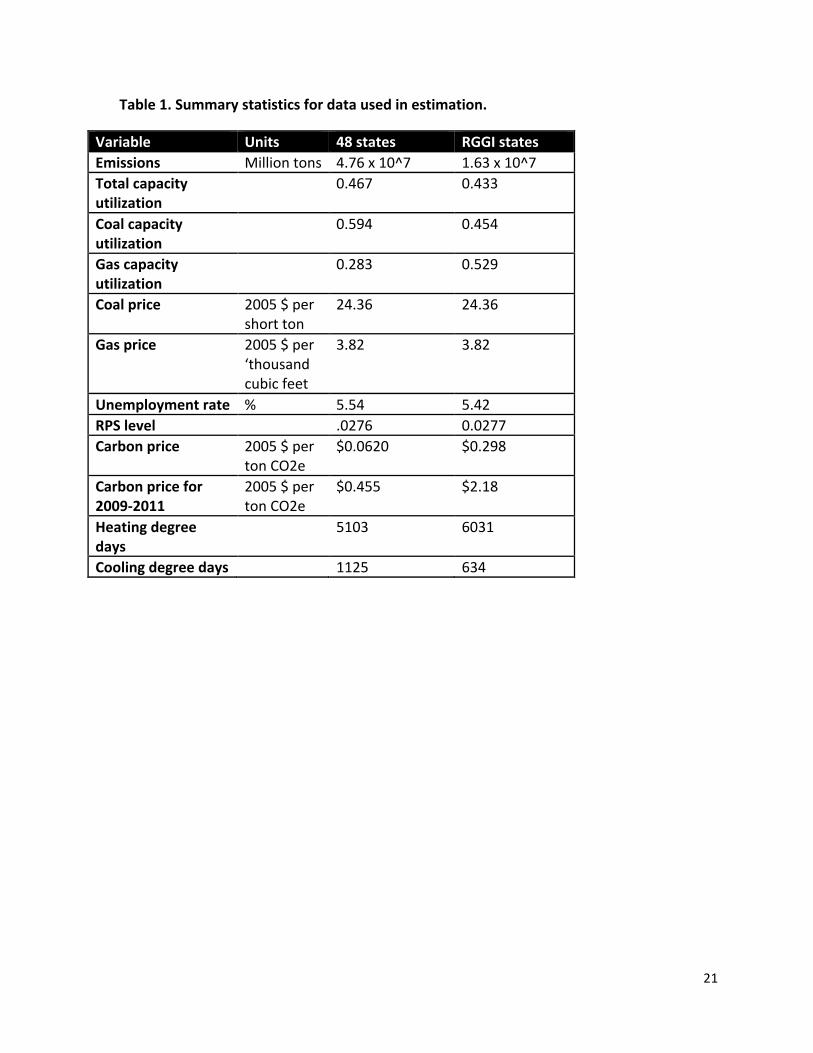
Our econometric model uses state-‐year data, largely from the U.S. Energy Information Administration (EIA 2013). They provide state-‐year data on CO2 emissions, total electricity generation, generation by fuel type, total generation capacity, generation capacity by fuel type, annual natural gas wellhead prices, and annual coal prices.5 Annual price indices are from the Bureau of Economic Analysis while unemployment statistics are from the Bureau of Labor tatistics. RPS data is from the Database of State Incentives for Renewable Energy (DSIRE). Annual carbon prices are the average of clearing prices of carbon allowance auctions held in each year; auction clearing prices are available from RGGI. Finally, weather data is available from the National Climatic Data Center (BEA, BLS, DSIRE, NCDC, RGGI).

Summary statistics are presented in Table 1 for all 48 continental states and the ten RGGI states.

Stationarity Tests As is well known, estimation based on nonstationary time series can lead to spurious results (Kennedy 2008). However, many series can be rendered stationary by removing a time trend. Fisher-‐style unit root tests (which run a unit root test on each panel and then jointly test the results) with Phillips-‐Perron tests with two lags on each group cannot reject the null of stationarity for total utilization rates (Choi 2001). However, the same tests do reject the null for the total, coal, gas and oil utilization rates at the 1% level after detrending. Thus the use of detrended data in our estimations. Natural gas generators make more use of spot markets. Gas is primarily distributed via pipeline, and thus there may be temporary local or regional shortages or gluts induced by limited pipeline capacity. Nonetheless, local gas prices are driven by broader spot prices and thus spot price are a reasonable measure. Furthermore national price indices ameliorates concerns that fuel prices would be endogenous to local production needs.

11

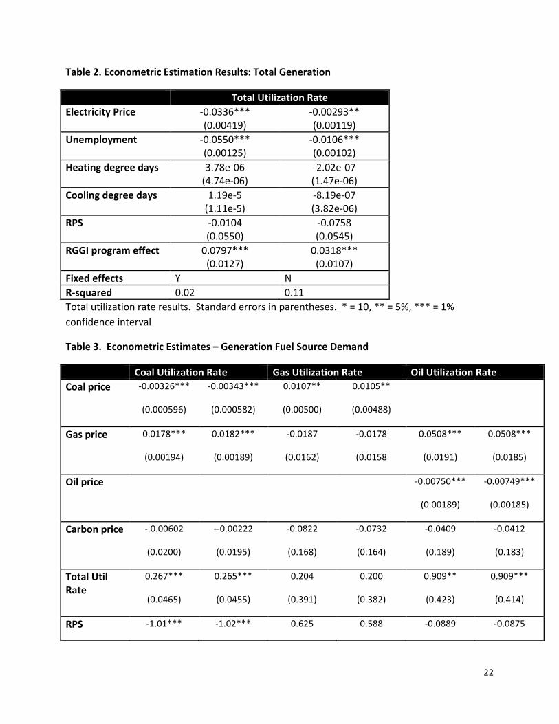
Estimation Results Estimation results are below in Tables 2 through 4. We report both random and fixed effects estimates for each model. We will use fixed effects results for simulations as not all random effects models passed Hausman specification tests for random effects (Hausman 1978).

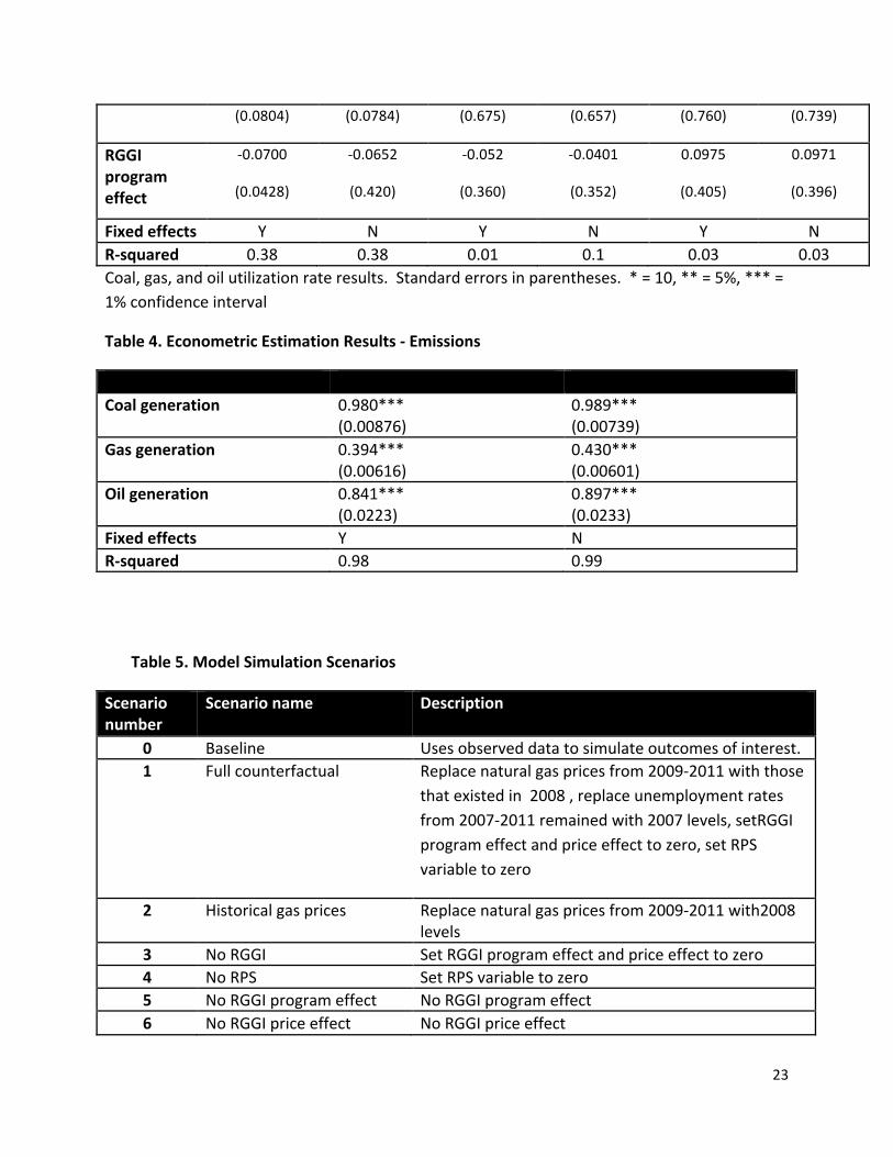
Most of the econometric estimates comport with theoretical expectations on sign. For instance in the generation demand equation (Table 3), own-‐price effects are negative, higher unemployment reduces demand, and weather variables have expected effects (the more cooling and heating degree days in a state/year, the more power demand), though this is only marginally significant statistically. The RGGI program variable seems to have a positive effect on total utilization rate, which is somewhat surprising given the energy efficiency expenditures associated with the program. 6 The generation fuel source demand equations (Table 4) also comport largely with expectations – own price effects are negative and cross-‐price effects with competing fuels are positive, individual fuel source utilization varies more strongly with total utilization for base load power such as coal than for gas, which often is utilized to hit peak demand. Coal utilization is lower in proportion to a state’s RPS requirements. On the contrary, the impact of an RPS on oil generation is near zero. This makes sense as oil generation is primarily used for peaking generation during very high demand. The effects of RPS on gas generation are statistically insignificant and somewhat ambiguous given the direct competition and renewables on one hand, but the differences in th use of each for base and peak load on the other. Carbon prices reduce fossil generation, but the effects are small and statistically insignificant because the prices themselves are low, for reasons discussed above. The emissions equation estimates (Table 5) line up perfectly with expectation, with coal and oil having more than double the emissions impact of gas.

In considering these results, the reader could be concerned about a lack of precision in some point estimates. However, note that estimates which we would think would have the biggest impact are quite precisely estimated – for example, price elasticities. Similarly note that the impact of an RPS is indistinguishable from unity on coal, implying that renewables nearly entirely substitute for coal base load. This is both quite precise and reassuring for our purposes as coal has the greatest emissions per unit of generation.

6 Additional analyses suggest that there has been a modest decline in the scale of generation under RGGI. This reduces both the numerator and denominator of the total utilization rate, resulting in a theoretically ambiguous sign. Analyses which estimate the level of total generation based on a similar set of covariates (interacted with population to control for state size) show more intuitive point estimates and qualitatively similar counterfactual simulation results.

12

Results of Simulation Exercise for Emissions Attribution

The model simulation scenarios are detailed in Table 5. We can then attribute the effect of different policies and market shocks by taking the difference between each scenario’s emissions and baseline emissions.

For each simulation, we first calculate the simulated statewide capacity utilization factor and fuel-‐specific capacity factors but based on counterfactual data, as defined in Table 6. Note that these are identical to equations 1 and 2 except that they omit the unobservable error term and add the time trend θ back in.

𝑐!" = 𝑋!"𝛽 + 𝜃!𝑡 + 𝜇! [1’]

𝑓!!" = 𝑌!Θ+ 𝑍!"Γ+ 𝜃!𝑡 + 𝜈! [2’]

We then calculate the generation level of each fuel by multiplying the capacity factor times the capacity (measured in megawatt hours) times the number of hours in a year (8760 for most year, 8784 for leap years) and use this to simulate the emissions based on equation [3

𝑚!" = 𝑉!"Κ+ 𝜉! [3’]

In each case, the coefficients are those estimated and reported in Tables 3 through 5. Simulations were developed for all “Lower 48” states as these data were all used for the econometric estimation, but most simulation results are reported here for RGGI states only, given the policy focus of the paper.

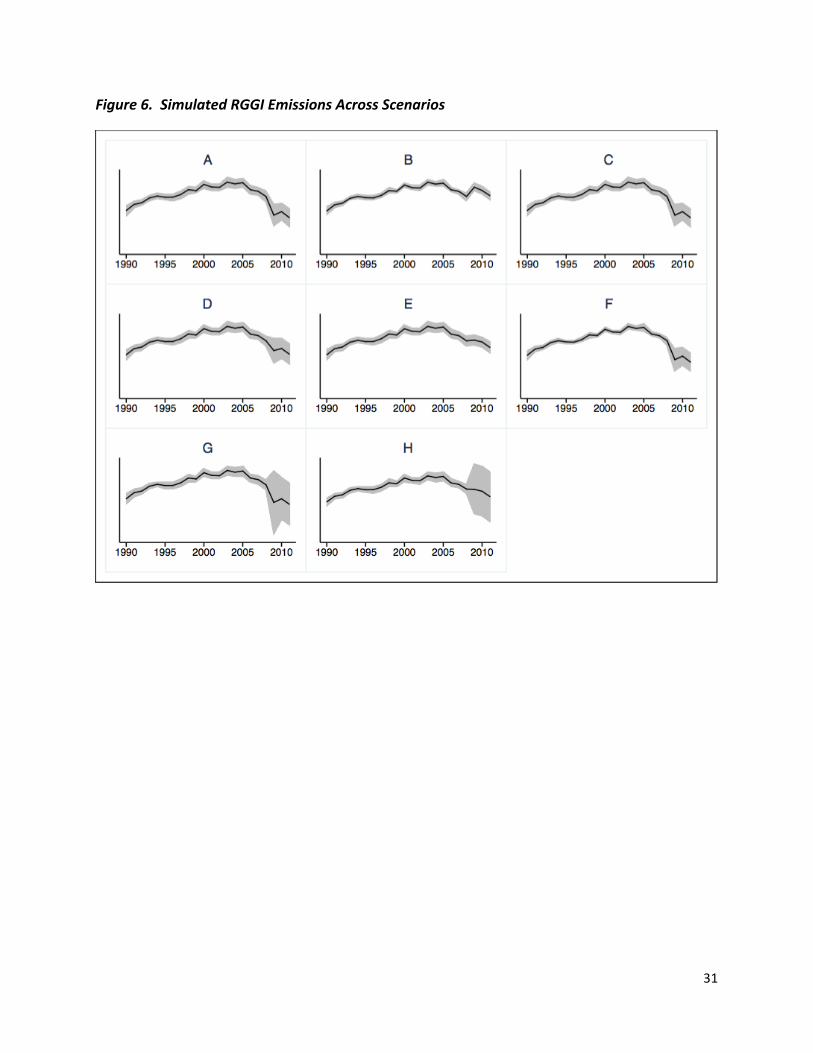
Figure 6 shows total RGGI state emissions for each scenario over time in red, with the 95% confidence intervals shaded. Panel A shows the simulated baseline, panel B the full counterfactual scenario, panel C the no recession scenario, panel D the historic gas price scenario, panel E the no RGGI scenario, panel F the no RPS scenario, panel G the no RGGI program effect scenario, and panel H the no RGGI price effect scenario. Note that the RGGI program commenced in 2009 and continues through 2011, our last data year. In our “full counterfactual” scenario, emissions across the 2009-‐2011 period remained near their mid-‐2000’s (pre-‐RGGI) peak. The simulations suggest that much of the decline is attributable to RGGI program effects even after controlling for other factors such as the recession, natural gas prices and RPS. Emissions declined much less in the “no RGGI” scenario than under the baseline. However, we cannot strongly distinguish the RGGI carbon price effect from a RGGI programmatic effect – see the broad confidence intervals for the program and price effects but the relatively narrow one for the joint effect. Emissions under our “historic gas prices” scenario were also higher, suggesting that reduced natural gas prices did play a role in reducing emissions.

13

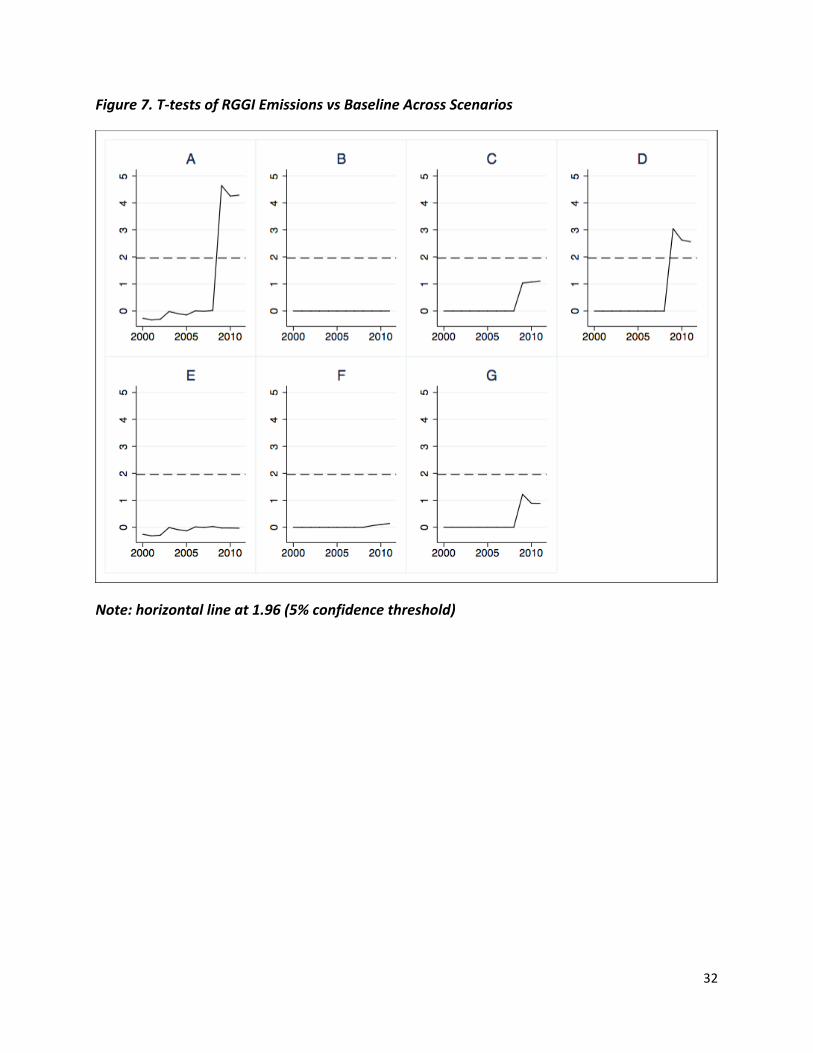
Figure 7 shows a t-‐test for the difference between the simulated emissions and baseline emissions for each scenario along with a horizontal line at 1.96 representing the standard 5% confidence level. Panel A shows the full counterfactual scenario, panel B the no recession scenario, panel C the historic gas price scenario, panel D the no RGGI scenario, panel E the no RPS scenario, panel E the no RGGI program effect scenario, and panel F the no RGGI price effect scenario. We see that the emissions in our “full counterfactual” and “no RGGI” scenarios were statistically distinct from the baseline showing that the collective influence of RGGI, natural gas prices, RPA and the economy lead to a statistically significant decline in emissions in the region, as did the isolated effect of the RGGI program alone, all else equal.

The impact of the recession alone on emissions was both economically modest and statistically insignificant. This is due to the low elasticity of total generation (total utilization rate) with respect to the macroeconomic indicator used (state unemployment rate).

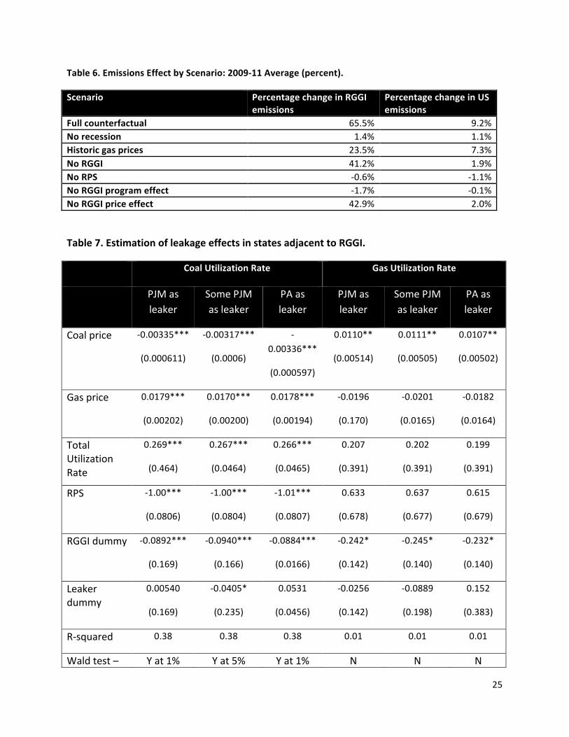
Table 6 summarizes the attribution of emissions effects in 2009-‐11. For each scenario, it shows the percentage difference between emissions under that scenario and baseline emissions for both the RGGI region and the entire US. Most of the reduction in emissions can be attributed to the RGGI program, although the dramatic decrease in gas prices also played a major role. The effect of the recession was neither economically substantial nor statistically significant. Interestingly, the dramatic decrease in gas prices had a bigger effect on emissions in the RGGI region than nationally. This could be because the RGGI region is so close to Pennsylvania, a center of the recent expansion in gas production.

Testing for evidence of leakage One potential explanation for why RGGI emissions have declined is that generation and emissions have shifted to non-‐RGGI states. If it is due to the policy, this is called “leakage”. Studies of leakage of subnational policies in other contexts have shown leakage rates of up to 70% and that regulations which place compliance costs on producers in a market-‐based setting (such as generators in electricity markets) are particularly likely to lead to leakage (Goulder 2012, Bushnell 2008). Evidence for the existence of leakage from RGGI is mixed – Shawhan et al (2014) use ex ante simulation methods and find that leakage would occur, while RGGI (2013) found no ex post statistical evidence of leakage.

Natural gas production increased dramatically over our study period to due technological advances in production technology (fracking). This increase was particularly dramatic in Pennsylvania, not a RGGI state itself, but it shares a border with RGGI states to the

14

north, east, and south.7 This increase in gas production lead to lower gas prices and fuel switching from coal to gas generation. We find evidence that coal generation decreased significantly and substantially more in RGGI states than in other nearby states. This suggests that gas-‐based electricity may have been preferentially exported to RGGI states, perhaps due to the RGGI program regulating emissions within its borders. We note however that preferential exports could also be affected by transmission limits, electricity price differentials, or other factors and leave it to future research to differentiate between these factors.

To test for leakage, we consider three different sets of potential “leaker” states. In the first we consider the member states of PJM, an electric power regional transmission organization (RTO) that coordinates the distribution of wholesale electricity in all or parts of 13 eastern U.S. states and the District of Columbia, which are not in RGGI (some PJM states are in RGGI, some are not). In the second case, we consider a limited set of PJM states – Ohio, Pennsylvania, West Virginia, and Virginia. These states are closer to RGGI than other PJM members and thus potentially would have more tightly linked electricity grids. In the third case we consider only Pennsylvania. For each of these potential leakers, we reestimate the econometric equations for coal and gas [Eq 2] adding in dummy variables which are 1 for potential leaker states during the RGGI compliance period. These dummies variables are detrended in keeping with the rest of the estimation. All specifications in Table 7 include fixed effects and omit the carbon price so as to more clearly compare treatment effects.

Note that for all three specifications of leakers, the coal utilization rate declined by more in RGGI states than in the leakers and that the difference was statistically significant. While gas utilization rate also declined by more in RGGI states, this difference was not statistically significant in any specification. These results provide some evidence of RGGI induced leakage effects. A more robust assessment of the nature and specific attribution of these effects is beyond the scope of this paper but would make an excellent topic of further research.

We make a back-‐of-‐the-‐envelope calculation of the potential emissions implications of this leakage by assuming that the entire difference between the utilization rates inside and outside RGGI were due to leakage. We do this for coal and gas and for coal alone. These calculations should be viewed as illustrative only. The gas calculation in particular is likely quite high as there have been reports that pipeline capacity constraints have limited gas shipments into parts of the RGGI region, and again the difference in point estimates is not statistically significant.8 Caveats aside, using the “PJM as leaker” specifications, if the entire difference

7 New Jersey has since left the program, but was in the program through 2011, which is the time period covered by this study. 8 EIA Today In Energy: New England spot natural gas prices hit record levels this winter. http://www.eia.gov/todayinenergy/detail.cfm?id=15111 accessed 4/18/2014

15

between the RGGI effect and the leaker effect were indeed due to leakage, the coal leakage would constitute 9.2 percent of RGGI region emissions over the period 2009-‐2011, while the coal and gas leakage combined would constitute 39.5 percent of emissions. This is greater than the entire reduction in emissions under the RGGI program. Policy leakage is plausible, consistent with observed generation and emission outcomes, and potentially of economically significant magnitude.

Conclusions and Policy Implications (BCM)

The end of the first decade of the 21st century provided an unusual time window to discern how different policy, technology and market factors influenced greenhouse gas emissions in the United States. During this period, policies were emerging at different levels of government to directly reduce GHGs or indirectly reduce them through complementary measures such as renewable portfolio standards and energy efficiency programs. At the same time, technological breakthroughs in hydraulic fracturing and horizontal drilling lead to a surge of new accessible natural gas reserves, lower prices and expanded use, especially in the northeastern U.S., where this study is focused. The switch on the margin from higher emitting coal to lower emitting gas has reduced the emissions intensity of electricity production. Added to the mix, the late 2000s brought the deepest economic recession in the U.S. since the 1930s, a factor that also contributed to a decline in emissions.

While many researchers and industry observers agree that all of these factors – policies, markets and macroeconomic conditions -‐ contributed to the decline in emissions experienced after 2008 in the U.S., there is little to no empirical evidence of how much each of these factors individually contributed to the decline. This lack of specific evidence is particularly important for the 10 northeastern states that comprised the Regional Greenhouse Gas Initiative (RGGI) that formed during the middle of the last decade and went into full effect in 2009. The RGGI states experienced a far more dramatic decline in emissions in the electric power sector (the nation’s largest source of emissions) than the rest of the U.S., which could be attributable to: the RGGI program itself which directly regulated GHG emissions from electric power, other policies, the fact that these 10 states were at or near the epicenter of the natural gas resource surge, or asymmetric effects of the economic recession on this region. An ability to attribute these effects to the different factors is particularly important in this region because of the magnitude of the decline and because of the uniqueness of the policy experiment there.

This study attempts to rectify this shortcoming by linking a conceptual framework of the cap-‐and-‐trade program developed under RGGI to an econometric model of the U.S. electric power sector that estimates state-‐level power generation demand, fuel mix and emissions. We use the

16

econometric model to develop counterfactual simulations to attribute, ex post, the factors driving emissions trends. For the RGGI states we find the following key results:

-‐ Power sector emissions would be more than 50% higher by 2011 in RGGI states were it not for the combination of policy, natural gas market and macroeconomic factors that emerged in the late 2000s.

-‐ Looking at individual factors, the economic recession had a very small influence on the emissions decline during this period (only about 1 percent of the emissions decline)

-‐ Natural gas markets were responsible for more than one-‐third of the emissions decline via induced substitution in the generation mix from higher emitting fossil fuels to natural gas

-‐ Controlling for the factors just referenced, the RGGI program itself appears to be the dominant factor in the emissions decline. It is difficult to statistically separate the effects of the RGGI price from other programmatic aspects such as the use of RGGI auction proceeds for energy efficiency and other low-‐carbon investments, but given the low RGGI price, and the regional effects appeared to commence once the program was announced and before trading started, the complementary program effects may be the key factor. More research is needed to explore the causes further.

-‐ Some or all of the reduction in RGGI emissions may be countered by generation and emissions leakage to surrounding states. We conducted an econometric analysis on spillover effects in states adjacent to the RGGI states who are part of the same regional transmission organization. The analysis suggests that the adjacent non-‐RGGI states may have picked up generation, especially from coal, that was diverted because of the RGGI program. Back-‐of-‐the-‐envelope calculations show that this effect could be as large as the entire reduction in emissions under the RGGI program.

Taken together, we believe these results have important policy implications. First, there appears to be substantial room for emissions reduction in electric power generation. Given this sector accounts for more than one-‐third of national emissions in the United States, this has implications for U.S. efforts to meet domestic and international global climate commitments. The results also suggest that a tightly targeted cap-‐and-‐trade program like RGGI can be effective at reducing emissions through a combination of the emissions trading elements and other programmatic elements that incentivize energy efficiency and reduced carbon intensity of electric power. This has implication for the state of California, who in 2013 instituted a multi-‐sector cap-‐and-‐trade program to help meet its GHG reductions under state law, as well as its recent efforts to link their carbon market to the Canadian province of Quebec.

17

The results also strongly point to the critical role that natural gas discoveries have played in reducing emissions. Natural gas, even before the recent surge in availability, has been viewed as a “bridge strategy” to a lower-‐carbon future, given its lower carbon content per unit energy than coil and oil. That crossing of that bridge has begun, but it awaits to be seen what is on the other side. Will demand surge so strongly causing a rise in prices that will put a brake on continued expansion and emission reductions on the margin? Will water quality and other environmental and safety concerns place limits on fracking and natural gas production? And how will even more ambitious targets for GHG reductions (e.g., more than 50% by mid-‐century) direct responses beyond natural gas, which is still a carbon emitter?

The results suggest that regional strategies can be effective in cutting emissions within a region, but the leakage analysis suggests that one consequence of improvements of one region targeted by policies is the possibility of shifting problems to other regions. As GHGs are a global pollutant, more comprehensive coverage is necessary for effective policy.

18

References

BEA. 2012. “NIPA tables: Table 1.1.4. Price Indexes for Gross Domestic Product.” Washington, D.C.

BLS. 2013. Local Area Unemployment Statistics Home Page. Washington, D.C. Retrieved from http://www.bls.gov/lau/ “Annual Average: Statewide data: Tables”

Bushnell, J, Peterman, C., Catherine Wolfram, C. 2008 Local Solutions to Global Problems: Climate Change Policies and Regulatory Jurisdiction. Review of Environmental Economics & Policy 2 (2): 175-193

Chevallier, Julien. 2011. “A model of carbon price interactions with macroeconomic and energy dynamics” Energy Policy 33(6): 1295–1312

Choi, I. 2001. Unit root tests for panel data. Journal of International Money and Finance 20: 249-‐272.

DSIRE. 2013. “DSIRE Quantitative RPS Data Project Database of Energy Efficiency, Renewable Energy Solar Incentives, Rebates, Programs, Policy”. Raleigh, NC. http://www.dsireusa.org/rpsdata/index.cfm

EIA. 2013. “Net Generation by State by Type of Producer by Energy Source ” Washington, D.C. From http://www.eia.gov/electricity/data/state/

EIA. 2013. “Existing Nameplate and Net Summer Capacity by Energy Source, Producer Type and State” Washington, D.C. From http://www.eia.gov/electricity/data/state/

EIA. 2013. “U. S. electric power industry estimated emissions by state, back to 1990 ”. Washington, D.C. From http://www.eia.gov/electricity/data.cfm#elecenv

EIA. 2013. “U.S. Natural Gas Prices”. Washington, DC http://www.eia.gov/dnav/ng/ng_pri_sum_dcu_nus_a.htm

EIA. 2011. “Annual Energy Review”. “Table 7.9 Coal Prices, 1949-‐2011” Washington, DC

EIA. 2013. “Spot Prices for Crude Oil and Petroleum Products.” Washington, DC http://www.eia.gov/dnav/pet/pet_pri_spt_s1_a.htm

Ellerman and Buchner (2008). “Over-‐Allocation or Abatement? A Preliminary Analysis of the EU ETS Based on the 2005-‐06 Emissions Data.” Environmental and Resource Economics (2008) 41:267-‐287.

Environment Northeast, 2011 (January). RGGI Emissions Trends. http://www.env-‐ne.org/public/resources/pdf/ENE_RGGI_Emissions_Report_120110_Final.pdf

19

Galperin. 2011. “The RGGI Emissions Cap: Is it too Forgiving?” On the Environment. Yale Center for Environmental Law and Policy. April 1, 2011. http://environment.yale.edu/envirocenter/the-‐rggi-‐emissions-‐cap-‐is-‐it-‐too-‐forgiving

Hausman, J. A. 1978. Specification tests in econometrics. Econometrica 46: 1251–1271.

Hibbard, Paul J. et al., 2011. The Economic Impacts of the Regional Greenhouse Gas Initiative on Ten Northeast and Mid-‐Atlantic States. Published by The Analysis Group, available at http://www.analysisgroup.com/uploadedFiles/Publishing/Articles/Economic_Impact_RGGI_Report.pdf

Goulder, L., Jacobson, M., van Bentham, A., 2012. Unintended Consequences from Nested State & Federal Regulations: The Case of the Pavley Greenhouse-‐Gas-‐per-‐Mile Limits Journal of Environmental Economics and Management, Vol. 63, No. 2

Kennedy, Peter. 2008. A Guide to Econometrics. Blackwell Publishing, Malden, MA.

Legrand, Marc. 2013. “The Regional Greenhouse Gas Initiative: Winners and Losers .” Columbia Journal of Environmental Law (24 April, 2013). http://www.columbiaenvironmentallaw.org/articles/the-‐regional-‐greenhouse-‐gas-‐initiative-‐winners-‐and-‐losers

Montgomery, W.D. 1972. "Markets in Licenses and Efficient Pollution Control Programs". Journal of Economic Theory 5: 395–418

Moomaw, W., P. Burgherr, G. Heath, M. Lenzen, J. Nyboer, A. Verbruggen, 2011: Annex II: Methodology. In IPCC Special Report on Renewable Energy Sources and Climate Change Mitigation [O. Edenhofer, R. Pichs-‐Madruga, Y. Sokona, K. Seyboth, P. Matschoss, S. Kadner, T. Zwickel, P. Eickemeier, G. Hansen, S. Schlömer, C. von Stechow (eds)], Cambridge University Press, Cambridge, United Kingdom and New York, NY, USA Murray, B.C, R.G. Newell, and W.A. Pizer. 2009. “Balancing Cost and Emissions Certainty: An Allowance Reserve for Cap-‐and-‐Trade.” Review of Environmental Economics and Policy 3(1): 84-‐103

NCDC. 2012. “Divisional Data Select” from http://www7.ncdc.noaa.gov/CDO/CDODivisionalSelect.jsp

Potential Gas Committee, 2009. Potential Supply of Natural Gas in the United States (December 31, 2008). Potential Gas Agency, Colorado School of Mines, Golden, CO.

20

RGGI, 2013. “CO2 Emissions from Electricity Generation and Imports in the Regional Greenhouse Gas Initiative: 2011 Monitoring Report.” Available at http://www.rggi.org/docs/Documents/Elec_monitoring_report_2011_13_06_27.pdf accessed 4/4/2014

RGGI, 2014. Regional Greenhouse Gas Initiative Fact Sheet. http://www.rggi.org/design/overview/cap/ (accessed March 27, 2014)

RGGI, 2014. Allowances Offered and Sold by Auction. http://www.rggi.org/market/co2_auctions/results (Accessed March 27, 2014)

Shawhan, D.L, Taber, J.T., Shi, D., Zimmerman, R.D., Yan, Jubo, Marquet, C.M., Qi, Y., Mao, M., Schuler, R.E., Schulze, W.D., Tylavsky, D. 2014. “Does a detailed model of the electricity grid matter? Estimating the impacts of the Regional Greenhouse Gas Initiative” Resournce and Energy Economics 36(1): 191-‐207

Stavins, Robert N. "Low Prices a Problem? Making Sense of Misleading Talk about Cap-‐and-‐Trade in Europe and the USA." Web log post. An Economic View of the Environment. Harvard University Kennedy School Belfer Center for Science and International Affairs, 25 Apr. 2012. Web. 9 Aug. 2012. http://www.robertstavinsblog.org/2012/04/25/low-‐prices-‐a-‐problem-‐making-‐sense-‐of-‐misleading-‐talk-‐about-‐cap-‐and-‐trade-‐in-‐europe-‐and-‐the-‐usa/.

Tietenberg, Tom H. 2013. “Reflections – Carbon Pricing in Practice.” Review of Environmental Economics and Policy 7(2): 313-‐329. US EIA. Average annual prices for coal and natural gas. Release dates: (Coal December 12, 2013 http://www.eia.gov/coal/data.cfm#prices) Natural gas (wellhead) http://www.eia.gov/dnav/ng/hist/n9190us3A.htm Feb 28, 2014)

21

Table 1. Summary statistics for data used in estimation.

Variable Units 48 states RGGI states Emissions Million tons 4.76 x 10^7 1.63 x 10^7 Total capacity utilization

0.467 0.433

Coal capacity utilization

0.594 0.454

Gas capacity utilization

0.283 0.529

Coal price 2005 $ per short ton

24.36 24.36

Gas price 2005 $ per ‘thousand cubic feet

3.82 3.82

Unemployment rate % 5.54 5.42 RPS level .0276 0.0277 Carbon price 2005 $ per

ton CO2e $0.0620 $0.298

Carbon price for 2009-‐2011

2005 $ per ton CO2e

$0.455 $2.18

Heating degree days

5103 6031

Cooling degree days 1125 634

22

Table 2. Econometric Estimation Results: Total Generation

Total Utilization Rate Electricity Price -‐0.0336***

(0.00419) -‐0.00293** (0.00119)

Unemployment -‐0.0550*** (0.00125)

-‐0.0106*** (0.00102)

Heating degree days 3.78e-‐06 (4.74e-‐06)

-‐2.02e-‐07 (1.47e-‐06)

Cooling degree days 1.19e-‐5 (1.11e-‐5)

-‐8.19e-‐07 (3.82e-‐06)

RPS -‐0.0104 (0.0550)

-‐0.0758 (0.0545)

RGGI program effect 0.0797*** (0.0127)

0.0318*** (0.0107)

Fixed effects Y N R-‐squared 0.02 0.11 Total utilization rate results. Standard errors in parentheses. * = 10, ** = 5%, *** = 1% confidence interval

Table 3. Econometric Estimates – Generation Fuel Source Demand

Coal Utilization Rate Gas Utilization Rate Oil Utilization Rate Coal price -‐0.00326***

(0.000596)

-‐0.00343***

(0.000582)

0.0107**

(0.00500)

0.0105**

(0.00488)

Gas price 0.0178***

(0.00194)

0.0182***

(0.00189)

-‐0.0187

(0.0162)

-‐0.0178

(0.0158

0.0508***

(0.0191)

0.0508***

(0.0185)

Oil price -‐0.00750***

(0.00189)

-‐0.00749***

(0.00185)

Carbon price -‐.0.00602

(0.0200)

-‐-‐0.00222

(0.0195)

-‐0.0822

(0.168)

-‐0.0732

(0.164)

-‐0.0409

(0.189)

-‐0.0412

(0.183)

Total Util Rate

0.267***

(0.0465)

0.265***

(0.0455)

0.204

(0.391)

0.200

(0.382)

0.909**

(0.423)

0.909***

(0.414)

RPS -‐1.01*** -‐1.02*** 0.625 0.588 -‐0.0889 -‐0.0875

23

(0.0804) (0.0784) (0.675) (0.657) (0.760) (0.739)

RGGI program effect

-‐0.0700

(0.0428)

-‐0.0652

(0.420)

-‐0.052

(0.360)

-‐0.0401

(0.352)

0.0975

(0.405)

0.0971

(0.396)

Fixed effects Y N Y N Y N R-‐squared 0.38 0.38 0.01 0.1 0.03 0.03 Coal, gas, and oil utilization rate results. Standard errors in parentheses. * = 10, ** = 5%, *** = 1% confidence interval

Table 4. Econometric Estimation Results -‐ Emissions

Coal generation 0.980***

(0.00876) 0.989*** (0.00739)

Gas generation 0.394*** (0.00616)

0.430*** (0.00601)

Oil generation 0.841*** (0.0223)

0.897*** (0.0233)

Fixed effects Y N R-‐squared 0.98 0.99

Table 5. Model Simulation Scenarios

Scenario number

Scenario name Description

0 Baseline Uses observed data to simulate outcomes of interest. 1 Full counterfactual Replace natural gas prices from 2009-‐2011 with those

that existed in 2008 , replace unemployment rates from 2007-‐2011 remained with 2007 levels, setRGGI program effect and price effect to zero, set RPS variable to zero

2 Historical gas prices Replace natural gas prices from 2009-‐2011 with2008 levels

3 No RGGI Set RGGI program effect and price effect to zero 4 No RPS Set RPS variable to zero 5 No RGGI program effect No RGGI program effect 6 No RGGI price effect No RGGI price effect

24

25

Table 6. Emissions Effect by Scenario: 2009-‐11 Average (percent).

Scenario Percentage change in RGGI emissions

Percentage change in US emissions

Full counterfactual 65.5% 9.2% No recession 1.4% 1.1% Historic gas prices 23.5% 7.3% No RGGI 41.2% 1.9% No RPS -‐0.6% -‐1.1% No RGGI program effect -‐1.7% -‐0.1% No RGGI price effect 42.9% 2.0%

Table 7. Estimation of leakage effects in states adjacent to RGGI.

Coal Utilization Rate Gas Utilization Rate

PJM as leaker

Some PJM as leaker

PA as leaker

PJM as leaker

Some PJM as leaker

PA as leaker

Coal price -‐0.00335***

(0.000611)

-‐0.00317***

(0.0006)

-‐0.00336***

(0.000597)

0.0110**

(0.00514)

0.0111**

(0.00505)

0.0107**

(0.00502)

Gas price 0.0179***

(0.00202)

0.0170***

(0.00200)

0.0178***

(0.00194)

-‐0.0196

(0.170)

-‐0.0201

(0.0165)

-‐0.0182

(0.0164)

Total Utilization Rate

0.269***

(0.464)

0.267***

(0.0464)

0.266***

(0.0465)

0.207

(0.391)

0.202

(0.391)

0.199

(0.391)

RPS -‐1.00***

(0.0806)

-‐1.00***

(0.0804)

-‐1.01***

(0.0807)

0.633

(0.678)

0.637

(0.677)

0.615

(0.679)

RGGI dummy -‐0.0892***

(0.169)

-‐0.0940***

(0.166)

-‐0.0884***

(0.0166)

-‐0.242*

(0.142)

-‐0.245*

(0.140)

-‐0.232*

(0.140)

Leaker dummy

0.00540

(0.169)

-‐0.0405*

(0.235)

0.0531

(0.0456)

-‐0.0256

(0.142)

-‐0.0889

(0.198)

0.152

(0.383)

R-‐squared 0.38 0.38 0.38 0.01 0.01 0.01

Wald test – Y at 1% Y at 5% Y at 1% N N N

26

leaker dummy different than RGGI dummy

Figure 1. Trends in Electricity Emissions and Determinants, RGGI States, 1990-‐2011. Index (1990=100)

27

Figure 2. Baseline Emissions, Cap, and Carbon Price

28

Figure 3. RGGI Auction 2008-‐13: Allowances Offered, Sold, and Clearing Price

Source: RGGI, 2014. Allowances Offered and Sold by Auction. http://www.rggi.org/market/co2_auctions/results

29

Figure 4. Coal and Natural Gas Nominal Prices Indexes (1990=100)

Source: Index derived using data from US EIA, Average annual prices for coal and natural gas. Release dates: (Coal December 12, 2013 http://www.eia.gov/coal/data.cfm#prices) Natural gas (wellhead) http://www.eia.gov/dnav/ng/hist/n9190us3A.htm Feb 28, 2014)

30

Figure 5. Electricity Generation by Source, RGGI States: 1990-‐2011

Source: US EIA (2013: Annual Power Generation Data by State, summed for RGGI states)

31

Figure 6. Simulated RGGI Emissions Across Scenarios

32

Figure 7. T-‐tests of RGGI Emissions vs Baseline Across Scenarios

Note: horizontal line at 1.96 (5% confidence threshold)