Embed Size (px)
Citation preview

SAFER, SMARTER, GREENER
WHITEPAPER
TRANSPORT LOGISTICS
Evaluation of the effect of different logistic conditions applied to oil supply chain

Prepared by DNV GL – Software
2017
© DNV GL AS. All rights reserved
This publication or parts thereof may not be reproduced or transmitted in any form or by any means, including copying or recording, without the prior written consent of DNV GL AS

| Whitepaper | Maros 9.3 | www.dnvgl.com/software Page i
Table of contents
1 INTRODUCTION .............................................................................................................. 1
2 SUPPLY CHAIN DEFINITION ............................................................................................. 1
2.1 Description of oil supply chain logistics 2
3 PERFORMANCE FORECASTING METHODOLOGY ................................................................... 4
4 CASE STUDY: FLOATING, PRODUCTION, STORAGE AND OFFLOADING .................................. 5
4.1 Description of digital twin 5
4.2 Maros for performance forecasting 5
5 RESULTS ..................................................................................................................... 14
6 SENSITIVITY ANALYSIS ................................................................................................. 19
6.1 Sensitivity 1: Operating rules 20
6.2 Sensitivity 2: Number of ships 22
7 CONCLUSION ............................................................................................................... 23
8 REFERENCES ................................................................................................................ 25

| Whitepaper | Maros 9.3 | www.dnvgl.com/software Page 1
1 INTRODUCTION
The petroleum industry is separated into three major operations: upstream, midstream and downstream
activities.
The upstream operation, also known as the exploration and production (E&P) sector, covers the
exploration, production and transportation of gas and crude oil from the oil fields to processing units,
where the final products are produced, mainly refineries and gas treatment facilities (GTF).
Midstream operations are commonly included as part of downstream operations for much of the oil and
gas industry. The midstream and downstream activities take place after the initial production phase and
through to the point of sale.
The downstream operation is a term commonly used to refer to the refining of crude oil and the selling
and distribution of natural gas and products derived from crude oil. Such products include liquefied
petroleum gas (LPG), liquefied natural gas (LNG) gasoline or petrol, jet fuel, diesel oil, other fuel oils,
asphalt and petroleum coke.
There is an important and common area to all operations: the transportation logistics. Basically, all
activities need to assess the level of product to be delivered. On the upstream operation, there is a need
to supply a certain amount of the oil and gas to the processing units or onshore storage terminals – a
failure during this stage of operation can directly impact the operation for the whole chain. On the
downstream operation, the transportation is even more important because the product is frequently
delivered directly to the end user.
Logistics play a big role in a company’s operation and are critical to the competitiveness of that company.
The demand for products can only be satisfied through the proper and cost-effective delivery of goods
and services.
Nowadays, logistics operations represent a big share of the market and the expenditures on these
operations are in the order of trillions of dollars annually.
Despite the recession in the United States in 2010, the logistics operations costs reached $1.2 trillion, an
increase of $114 billion from 2009. The number is even more incredible when evaluated by the
contribution on the nation’s gross domestic product (GDP). The logistics participation in the US economy
represents 8.3 per cent of the nation's gross domestic product (GDP) in 2010, compared with 7.8 per
cent in recession-wracked 2009.
In this scenario, where trillions of dollars are in place, even a small increase to the efficiency of deliveries
schedules and contracts represent a large amount of money.
2 SUPPLY CHAIN DEFINITION
The supply chain is defined as follows (Hugos, 2011):
“A supply chain consists of all stages involved, directly or indirectly, in fulfilling a customer request. The
supply chain not only includes the manufacturer and suppliers, but also transporters, warehouse,
retailers, and customers themselves.”

| Whitepaper | Maros 9.3 | www.dnvgl.com/software Page 2
The main difference between the concept of the supply chain and the logistics operation is the boundary
of each activity. Logistics operations are usually related operations that occur within a company
boundary whereas the supply chain represents a network of companies.
Taking this definition, a logistics operation evaluation must consider:
Customer contracts: this represents what the customers need of the product – in this case, crude
oil and gas. Usually, suppliers have several contracts with different customers for products with
different specifications. Managing all this contracts is one of the most difficult tasks in a logistic
assessment.
Buffer level management: the objective of buffer level management is to align and maintain the
lowest levels possible that will meet the contracts agreed with the customers.
Supply: the process of building inventory to the targets established in buffer level management
planning. Make sure the levels on tanks agree with what needs to be exported.
Transportation: physically links the sources of supply chosen in sourcing with the customers.
This involves many different resources that must be aligned to optimize efficiency.
Storage: in an ideal scenario where the activities above are well implemented, the storage
activity may be outsourced. However, a failure in a critical equipment of a platform might shut
down the production for days, stopping the whole process. Storage tanks increase the availability
of a certain product when demand increases or, in a case where the transfer is delayed, the
product can be held without the need to stop the whole system. It also allows more time for the
operator to adjust the product within a certain specification or, more related to the purpose of
this article, to prepare for expected or unexpected outages.
The focus of this article will be on the evaluation of different logistics conditions and how they have an
impact on the final production efficiency of the supply chain. The focus will be the transportation of oil
between the platforms to an intermediate storage farm tank.
2.1 Description of oil supply chain logistics
A simplified oil supply chain can be explained with the following parameters:
Platforms will produce crude oil
Transportation is typically performed by crude oil tankers or pipelines that deliver production to
tank farms
Tank farms feed refineries that will process crude oil to produce more valuable fractions of oil
Refined products are distributed to consumers
The starting point of the supply chain is the production of crude oil from offshore platforms. At this stage
of the supply chain, several factors can impact the supply chain efficiency. Failure of equipment items,
planned shutdowns and operational bottlenecks will cause disruption to the supply chain.
One important component of the supply chain that works as a mitigation to these events is the storage
tanks. Storage tanks play an important role because they can maintain production in case of a shutdown
upstream to the storage facility or maintain production from a platform in case an oil tanker is delayed
or there is an outage at the facility downstream to the storage tank.
In the context of being able to store products, Floating, Production, Storage and Offloading (FPSO)
platforms have a unique design. The basic design of most FPSOs is of a ship-shaped vessel, with

| Whitepaper | Maros 9.3 | www.dnvgl.com/software Page 3
processing equipment (or topsides) aboard the vessel's deck and hydrocarbon storage underneath the
deck, in a double hull arrangement. After processing, an FPSO stores oil and offloads periodically to
shuttle tankers or transmits processed petroleum via pipelines.
Taking the aforementioned example of upstream and downstream outages, the storage facility in the
FPSO plays a central role in its operation. A shutdown may cause problems upstream and downstream to
the storage facility leading to a full shutdown of the field. Upstream failures are typically related to
problems in the platform, but if the export system is still available and a carrier is loading, the system
might be able to complete the loading process before complete shutdown. In this scenario, the carrier
will only be able to take the product available in the storage facility. Downstream problems will cause an
interruption to the export system but production can be maintained up to the point where the storage
tank cannot take more production and a complete shutdown of the plant is required.
Thus, the best operational scenario is that the tanks never reach their maximum or minimum level limits.
In the oil supply chain, the platform feeds the tankers with oil, which is taken to the terminal where the
oil is exported. The export operation is carried out by crude oil tankers.
Among the main tanker classes are:
Table 1. Main tanker classes
Class Length Beam Draft Overview
Coastal
Tanker
205 m 29 m 16 m Less than 50,000 dwt, mainly used for transportation of refined
products (gasoline, gasoil).
Aframax 245 m 34 m 20 m Approximately 80,000 dwt (Average Freight Rate Assessment).
Suezmax 285 m 45 m 23 m Between 125,000 and 180,000 dwt, originally the maximum
capacity of the Suez Canal.
VLCC 330 m 55 m 28 m Very Large Crude Carrier. Up to around 320,000 dwt. Can be
accommodated by the expanded dimensions of the Suez Canal.
The most common length is in the range of 300 to 330 meters.
ULCC 415 m 63 m 35 m Ultra Large Crude Carrier. Capacity exceeding 320,000 dwt. The
largest tankers ever built have a deadweight of over 550,000
dwt.
Once the crude oil reaches the onshore terminal, it is typically fed to tank farms. There are basically
three fundamental operations to tank farms: import of crude oil, transportation between the tanks and,
finally, export of crude oil.
Tanks within tank farms are interconnected, which allows transport of products between tanks. This
procedure is carried out when there are several tanks half-empty and none available to receive the oil.
As tank farms normally receive more than one product, this operation must be carried out to avoid
contamination of products.
The export operations, from the tank farms to the refineries, are generally performed by pipelines.
Pipelines are the most efficient method to transport crude oil and refined products.

| Whitepaper | Maros 9.3 | www.dnvgl.com/software Page 4
Managing the supply chain of oil can be an extremely complex task. In addition to dealing with routine
operations such as planned turnarounds, the analysis must account for unplanned events such as ship
delays, power failures, weather problems and plant outages both in the export system. These events will
cause an interruption to the production to be transported, and it also makes carriers wait, which can lead
to severe penalties. It is important to note that being unable to meet a production demand will cause
direct financial impact, by losing revenue and payment of penalties, but can also cause problems to the
company’s image as an unreliable supplier.
Thus, understanding the risks in each step of the oil supply chain is essential to ensure a profitable and
reliable operation.
3 PERFORMANCE FORECASTING METHODOLOGY
Performance forecasting is a methodology that uses an “event-driven” algorithm based on Monte Carlo
simulation to create life-cycle scenarios of the system under investigation. This methodology is used to
predict the performance of an asset based on the reliability, availability, maintainability and operability of
the system.
A description of each one of these variables follows:
Reliability is the probability of an equipment/system to perform a required function under stated
conditions for a specified period of time.
Availability measures the time where equipment/system is actually operating. The calculation is
based on how often failures occur and how efficient corrective maintenance, taking into account
how quickly failures can be isolated and repaired. Preventive maintenance must also be taking
into account when evaluating the availability of an equipment/system. This can measure based
on how often preventative maintenance (schedule stoppage) is performed and how quickly these
tasks can be performed.
Maintainability is the ability of an equipment/system to be repaired to a specified condition when
maintenance is performed. The maintainability can consider all kind of resources e.g. like
number of personnel available, crew skills, spares, location of the repair, crew and spare.
Operability is the manner on how the system is operated; accounting for operability is essential
to correctly predict the performance of an asset in the oil and gas industry. The initial step when
modelling the operability of an oil and gas asset is accounting for the production profile of the
stream flowing through the system. For an upstream facility, this includes all the wells with
corresponding flow composition that will feed that platform – note that this behavior might be
transient due to phase-in and phase-out of wells throughout the life of the platform. By adding
the production rates, many operation rules can be defined such as degraded failures of
equipment where production is partially loss, production ramping time, storage facilities defined
with size, inflow and outflow, flaring operations and the transportation of the products.
This methodology can be applied during all different phases of a project: from the design phase, to
assess what would be the best technology to be implemented, to the operating phase, to check what the
bottlenecks in the process are and how failures affect the throughput of the unit.

| Whitepaper | Maros 9.3 | www.dnvgl.com/software Page 5
4 CASE STUDY: FLOATING, PRODUCTION, STORAGE AND
OFFLOADING
This study aims at verifying the impact logistics operations can have to the supply chain as a whole.
Here we will focus on transportation from offshore oil platforms to onshore oil storage terminals, which
deliver the oil to the refineries.
As the main purpose of this article is to show how constraints on the export operation can affect the
performance of the supply chain, it is assumed that the refinery does not have any failures during the
life of the system and the only constraint is related to the export operation.
From a basic crude oil processing unit different logistics profiles will be implemented, varying:
Transport resources: number of ships available
Buffer level operating rules
4.1 Description of digital twin
This case study investigates the transport logistics challenges of a Floating, Production, Storage and
Offloading (FPSO) platform. The system to be designed is expected to operate for 10 years. In this
model, the system design capacity is 400 mbbls per day and oil export system is 150 mbbls per day.
There are two oil well fields: Jupiter with two wells and Saturn with four wells; each field has one drilling
center. These wells have similar systems including valves, tubing, jumpers and manifolds. The
production from each field converges to the FPSO, which is then exported using tanker operations.
The FPSO includes a large range of different systems such as oil processing, gas compression and
dehydration, produced water, flare, vent and power generation. In addition to typical equipment failures,
there are losses associated to vessel motion preventing the export operation. The maintenance is
handled by a maintenance crew located on site at the FPSO and extra resources are needed depending
on the equipment failing.
4.2 Maros for performance forecasting
A virtual model of the production field is defined using a range of techniques. The software used to
create the digital twin of the production field is Maros.
Maros is a performance simulator that provides an objective, quantitative approach to systems' design.
Performance is a measure of a system's ability to reach its design requirements, which may be
productivity related, or the need to provide a specific service or function. Maros is an acronym for:
Maintainability, Availability, Reliability and Operability Simulation program.
Maros is a design tool that permits the development and comparison of systems by predicting their life-
cycle behavior pattern. Comparisons can be made of the most elementary concepts in the early stages of
a design project when few details are fixed (or known), while at the other extreme complex systems can
be optimized to yield maximum cost-efficiency. As its acronym suggests, the package encompasses well
known 'types' of analyses that have been successfully integrated into a simulation algorithm and offered
as a design aid. Users need not be specialists nor have an intimate understanding of the mathematics
involved. Emphasis is placed on 'engineering' a system to cope with its lifetime design requirements.
However, this life-cycle approach does introduce the need to consider maintenance and operations of the
system as well as its initial design layout.

| Whitepaper | Maros 9.3 | www.dnvgl.com/software Page 6
Maros was originally developed for the offshore oil and gas industry, where it has been used extensively
to design process facilities and transportation systems to exploit hydrocarbon reservoirs. It is, however,
a general-purpose systems design tool currently used in a wide range of applications including:
Chemicals
Power generation and distribution
Defense
Manufacturing
Transportation, etc.
Its particular applications involve the following aspects:
Equipment reliability and redundancy
Establishing maintenance and intervention strategies
System productivity and sales quotas
System operability assessment
Safety procedures
Risk analysis
Operations research
Maros was prototyped in 1984 and is under continual development.
The following chapter describes the modelling elements used to build the digital twin for this case study.
4.2.1 Block flow diagram
The first, and probably most important step in the modelling process, is to generate a block flow diagram.
The block flow diagram is a logic network that defines the connectivity of mass balance nodes and
focuses on the production aspects of the system. Each node within the network will require its own
reliability block diagram (RBD) that identifies how the system's components are logically connected, and
their operating mode.
Figure 1: Block flow diagram

| Whitepaper | Maros 9.3 | www.dnvgl.com/software Page 7
The dynamic behavior of an upstream system must also be considered. The model must be comprised of
planned changes in the system configuration, such as increasing production rates by commissioning
more wells to the system (or the inverse process when decommissioning wells).
Since commissioning or decommissioning wells will impact the production rates for each stream (oil,
water and gas), two streams are unlikely to maintain a constant ratio. Thus, the impact of failures on
processing equipment will have time variant impact.
For example, consider an oil field that starts its life producing 100 bbls per day and in the second year
there is a flow reduction to 50 bbls per day. Assuming this oil field is comprised of two pumps, and each
pump can handle 50% of the flow. In order to avoid bottlenecks in the system; these pumps must be
designed to take the peak capacity of the oil flowing through the platform. In this particular example, the
rate of 100 bbls per day is set for the first year. So handling 50% of flow means that each pump should
handle at least 50 bbls. This design is fixed, pumps with this capacity have to be purchased and their
capacities don’t change.
Now considering that one of pumps has a failure in the first year – this means that the system loses the
ability to produce at full capacity. Losing one pump means that the system loses the ability to produce
50 bbls per day; i.e. 50% of its capacity. So, the export capacity will be 50 bbls per day. Now assuming
that the same failure occurs five years later when the production has reduced to 50 bbls per day, the
impact will be 0% as the system can continue to work with one pump only. This is an example of a
system that starts its life under stress, with a 2X50% configuration, and toward the end of its life has
more spare capacity, in this case, showing 2x100% of configuration.
The same approach could be applied to different product streams. For example, for an upstream system,
we normally refer to oil, gas and water. Therefore, the compression system and the water production
system will have their production profile associated to them.
4.2.2 Production profile
The characteristics of oil/gas reservoirs are such that the feedstock is a finite and dwindling supply, and
the potential production decreases with time. Furthermore, it is common practice to build up initial
production to a plateau level; hence, initially the potential is low. A similar analogy could be the
expansion of a system to cope with increased demand of a product, e.g. phasing in new assembly lines,
process trains etc.

| Whitepaper | Maros 9.3 | www.dnvgl.com/software Page 8
The following figure describes the production profile considered for this case study.
Figure 2: Production profile
It is important to note the peak production of crude oil (150 mbbls per day) occurring during the first
year. This means the system will have almost no security margin (i.e. every event that causes shutdown
will be critical and produce direct production loss) or boost the system to compensate for production loss
scenarios.
4.2.3 Equipment failures
Equipment failures are defined using statistical distributions. These events are occurrences that cannot
be precisely defined in the timeline but can be estimated using probabilistic distributions. Two sets of
distributions are normally required to define a failure event: a failure distribution and a repair
distribution.
A failure distribution will be used to sample the time to failure and the repair distribution will be used to
define the duration of a repair task (without taking into account maintenance resource evaluation).
Figure 3. Example of failure distribution with MTTF of 1 year defined

| Whitepaper | Maros 9.3 | www.dnvgl.com/software Page 9
Figure 4. Example of repair distribution defined as rectangular distribution with minimum of
24 hours and maximum of 48 hours
The distributions commonly used to define failures are exponential, Weibull and Normal distributions. For
the repair distributions, the distributions commonly used are log-normal, rectangular and triangular.
This case study incorporates mainly reliability data from publicly available sources such as the OREDA
handbook and also factored data to account for the different operating conditions as well as
environmental changes (SINTEF, 1997).
An example of the reliability data defined for the chemical injection system is defined below:
Table 2. Example of reliability data used to describe the chemical injection system
System Equipmen
t item
Failure
mode
Capacit
y Loss
at
failure
Capacit
y Loss
at
repair
Failure
distributio
n
Mean
time
to
failure
(years
)
Repair
distributio
n
Mean
time
to
repair
(hours
)
Process
chemica
l
Injectio
n Pump
Injection
Pump
Critical 100% 100% Exponential 2.16 Constant
Repair Time 13
Degrade
d 0% 100% Exponential 0.83
Constant
Repair Time 8
Electric
motor
Injection
Pump
Unknow
n but
critical
failure
100% 100% Exponential 7.56 Constant
Repair Time 30
Degrade
d 0% 100% Exponential 10.51
Constant
Repair Time 23.8
4.2.4 Planned maintenance
Planned maintenance is defined as scheduled events. These events are occurrences that can be precisely
defined in the timeline with known frequency of occurrence and duration.

| Whitepaper | Maros 9.3 | www.dnvgl.com/software Page 10
A list of three preventive maintenance tasks is shown in the graph below. This graph shows these events
placed in a timeline (X axis) and the length of the box represents the duration.
Figure 5. Planned maintenance schedule
4.2.5 Maintenance resources
A maintenance crew is required to perform repairs for all the planned maintenance activities as well as
corrective maintenance.
4.2.6 Transport logistics
The transport logistics feature in Maros covers all types of transport systems that involve transfer of
products from suppliers to customers. The following common transport modes are catered for:
Rail Car
Barge
Ship
Road Tanker
Conceptually, the approach remains the same with products moving from a supplier (provider/seller) to
a customer (purchaser) via loading points (berths) using a fleet of transport resources.
The standard modelling approach for transport logistics in Maros is time-based, where physical routes
between the customer and suppliers are not important. In the time-based approach, travel times are
defined by the outbound and inbound travel time distributions and analysts can also define travel delays
using cumulative distribution functions.
The building of the logistics infrastructure is largely the same. There are three basic types of elements
relating to the bulk transport modelling. The following section describes each one of these elements:
| Whitepaper | Maros 9.3 | www.dnvgl.com/software Page 11
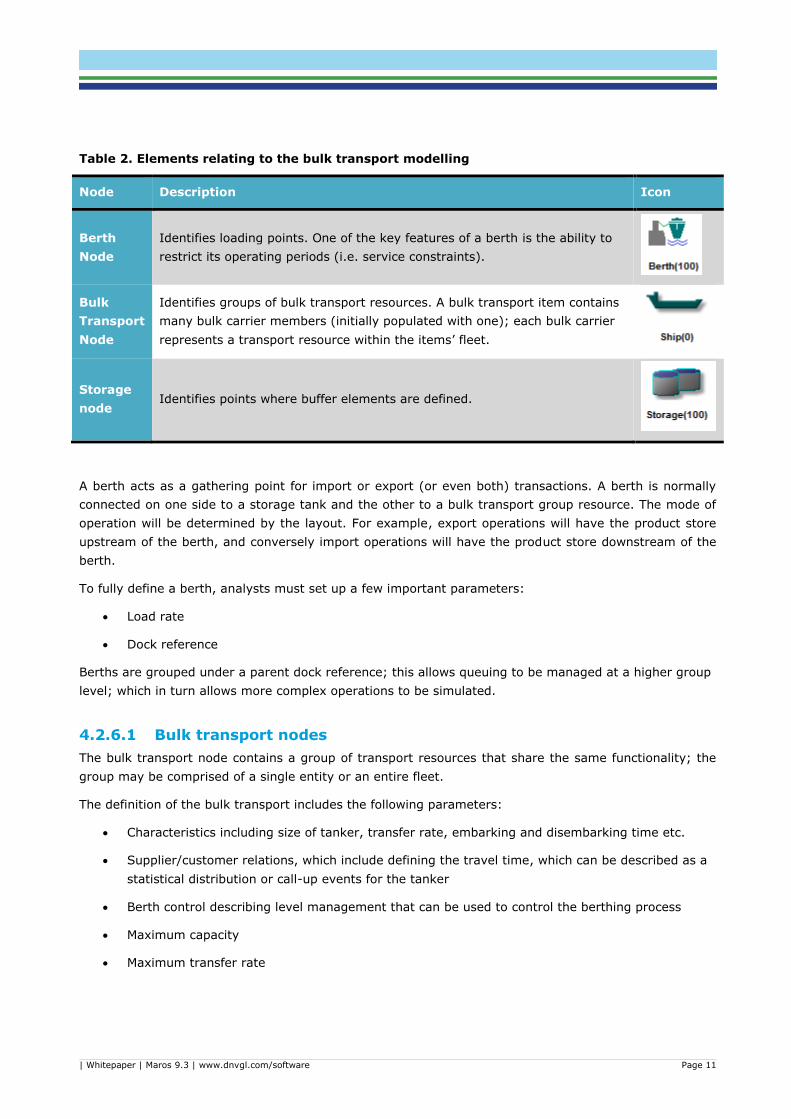
Table 2. Elements relating to the bulk transport modelling
Node Description Icon
Berth
Node
Identifies loading points. One of the key features of a berth is the ability to
restrict its operating periods (i.e. service constraints).
Bulk
Transport
Node
Identifies groups of bulk transport resources. A bulk transport item contains
many bulk carrier members (initially populated with one); each bulk carrier
represents a transport resource within the items’ fleet.
Storage
node Identifies points where buffer elements are defined.
A berth acts as a gathering point for import or export (or even both) transactions. A berth is normally
connected on one side to a storage tank and the other to a bulk transport group resource. The mode of
operation will be determined by the layout. For example, export operations will have the product store
upstream of the berth, and conversely import operations will have the product store downstream of the
berth.
To fully define a berth, analysts must set up a few important parameters:
Load rate
Dock reference
Berths are grouped under a parent dock reference; this allows queuing to be managed at a higher group
level; which in turn allows more complex operations to be simulated.
4.2.6.1 Bulk transport nodes
The bulk transport node contains a group of transport resources that share the same functionality; the
group may be comprised of a single entity or an entire fleet.
The definition of the bulk transport includes the following parameters:
Characteristics including size of tanker, transfer rate, embarking and disembarking time etc.
Supplier/customer relations, which include defining the travel time, which can be described as a
statistical distribution or call-up events for the tanker
Berth control describing level management that can be used to control the berthing process
Maximum capacity
Maximum transfer rate

| Whitepaper | Maros 9.3 | www.dnvgl.com/software Page 12
4.2.6.2 Connection arrangement
Several configurations can be used to model a logistic scenario, but the basic rules that should be
followed are:
A berth must be located both upstream and downstream of the oil carrier.
A tank must be provided both upstream and downstream of the berth.
Figure 6. Example of Connection arrangement
At start-up, the first bulk carrier commences loading at the supplier. Any other carriers within the group
(fleet) will be equally spaced out between leaving the customer side and the loading point. It may be
prudent to have an initial level in the import store, otherwise there will be no production taking place
until the first load is transferred to the import store.
Once loaded the carrier sets off for the customer using the outward-bound travel distribution. Operations
such as disembarking time can be modelled as there is a berth at the supplier side. On arrival at the
customer berth location the carrier will commence berthing if the following conditions are met:
The berth is not already in use by another carrier
The berth is open
There are no berth operation delays occurring
If any of the foregoing occurs the carrier is placed on the unload queue and will be eventually berthed in
the order in which it was placed in the queue.
Once berthed the unloading operations will commence if the following conditions are met:
The berth loading periods are active i.e. loading permitted
There are no equipment failures stopping the load transfer to the import store.
Once emptied, disembarking operations will take place if the following conditions are met:
There are no travel faults occurring
There are no berth operation delays occurring
On completion of the disembarking procedure the carrier is marked as being ready for another load and
immediately sent to the supplier for another load using the inbound travel distribution. If the supplier
side is busy on arrival the carrier is placed on the load queue and will eventually be loaded in the order
that it entered the queue.
4.2.6.3 Definition of the logistics operations
Initially, the model will assume a fleet that is composed of four crude oil carriers, each being able to
carry 3 million barrels; this falls within the category of ULCC. There are a small number of ULCC vessels
currently in use, as their size requires special facilities limiting the number of places where these vessels
can load and offload. These massive vessels can carry around 2 million barrels to 3.7 million barrels of

| Whitepaper | Maros 9.3 | www.dnvgl.com/software Page 13
crude oil. The size of the fleet is calculated based on the peak production of crude oil which occurs in
2060, the third year of production where all wells are commissioned. The timeline to complete a full
delivery is described as follows:
2 days to load
1 day to travel to the customer
2 days to unload the cargo
1 day to return to load more production.
It is expected that the operation is completed within 6 days when the oil tanker is back to the FPSO to
load more crude oil.
The simulation will try to optimize the number of crude oil carriers utilized throughout the life of the
asset. The model is defined with to allow overtaking in the export queue - this allows overtaking in the
queue in the export side for members of the same fleet only, such that the minimum numbers of
members in the fleet are used.
As mentioned before, only a few ports around the world have the infrastructure to accommodate a ULCC.
Thus, for this case study, it is assumed that only one port is available to receive the cargo. This port
operates between 6am and 6pm, which means that arrival and departure times will be restricted. The
restriction on the arrival and departure will impact the commencement of berthing and disembarking
operations. These operations cannot commence before the initial arrival time in any day and they must
be completed before the last departure time in any one day. Note that failure to complete either
operation will constitute a complete restart the following day, i.e. these operations cannot be suspended
and resumed the next day.
In addition to the travel time, defined as one day, the probability of the carrier being delayed is also
accounted for. This might be caused by metocean condition, vessel traffic etc. The probability of being
delayed is described as:
• There is 10% probability of being 1 day late
• There is 50% probability of being 0.5 day late
• There is a 40% probability of being 0.25 day late
Finally, the level of the storage facility is what controls the call-up of oil tanker. To fully define the buffer
level management rule, two values need to be defined in the threshold range. The first value (from)
indicates the percentage of the tank volume that will initiate the call-up. The second value indicates the
percentage of the tank volume that will end the call-up. Note that if a group of resources is loading at
the moment the call-up ends, the loading will be completed and the fleet will travel to its destination
before the tanker go back to the idle condition.
The following schematic shows how the software tool simulates the threshold being used:

| Whitepaper | Maros 9.3 | www.dnvgl.com/software Page 14
Figure 7. Operating rules description
In this case study, the range considered to operate the call-up of tanker is between 80% where the call-
up will be initiated and 70% where the call-up will be ended. These values are selected based on the
assumption that the likelihood of getting outages upstream the storage facility (i.e. the platform) is
much higher than downstream the storage facility (i.e. transport logistics).
5 RESULTS
The results of the model without the transport logistics modelled will be used to create a benchmark for
the study of the logistics operations.
The main key performance indicators used to compare the different cases are:
Production efficiency (or deliverability according to ISO 20815)
Annual production efficiency and volume per year
Average volume produced (mbbls) and product loss (mbbls)
Utilization of the oil tankers
Probability of non-exceedance curve for the storage tank
Where necessary, more results will be used to explain the behavior of the simulation.
The simulation is run for 100 cycles representing 100 feasible lives of the system.
Bulk TankerHigh Threshold
Low Threshold
Initiating BT call up
Ending BT call up
Call up of Bulk
Transport resources
initiated by a rising
level in a tank
Bulk TankerHigh Threshold
Low Threshold
Initiating BT call up
Ending BT call up
Call up of Bulk
Transport resources
initiated by a rising
level in a tank
Bulk Tanker
High Threshold
Low Threshold
Initiating BT call up
Ending BT call up
Call up of Bulk
Transport resources
initiated by a falling
level in a tank

| Whitepaper | Maros 9.3 | www.dnvgl.com/software Page 15
The production available for the system without the transport logistics modelled is: 89.65% with a
standard deviation of 1.1%. The average volume produced over the system life is 267,958 mbbls and
the average production loss is 30,939 mbbls.
The following graph shows the annual production efficiency and volume per year:
Figure 8. Annual production efficiency and volume for base case
The blue portion of the bar indicates the average production loss per year, whereas the green portion
shows the average volumetric production per year. It is important to note that during year 1 to 3, the
system is under stress with full capacity being utilized. That is why production loss is very critical at
these two periods of the life of the asset.
For the benchmark model, where no logistics operations are modelled, the Utilization of the oil tankers
and probability of non-exceedance curve for the storage tank are not available.
Now, by adding the logistics operations to the benchmark model, it is possible to isolate the impact of
constraints in the logistics to the overall system performance. The production availability when the
logistics are taken into consideration is: 87.368% with a standard deviation of 0.866%.; a reduction of
2.3% when compared to the base case.
The average volume produced over the system life is 261,141 mbbls and the average production loss is
37,756 mbbls. This represents a reduction of over 7,000 mbbls of transported product. Considering the
price for an oil barrel at USD$50, 00 per barrel, this represents a production loss of close to USD$680M –
this difference is displayed in the following graph:

| Whitepaper | Maros 9.3 | www.dnvgl.com/software Page 16
Figure 9. Compared cash-flow of base case with and without logistics
The annual production efficiency and volume per year shows a very similar pattern when compared to
the base case result:
Figure 10. Annual production efficiency and volume for base case with shipping
Cumulative Cash; -1276,968
Cumulative Cash; -1549,625-3000
-2500
-2000
-1500
-1000
-500
0
Cash
-flo
w (
US
D $
)

| Whitepaper | Maros 9.3 | www.dnvgl.com/software Page 17
The Utilization of the oil tankers is described by the following graph:
Figure 11. Utilization of carriers
It can be noted from the graph above that the Utilization of Carrier 1 is slightly higher when compared to
Carrier 2, 3 and 4 – remember that the simulation engine will try to optimize the number of the carriers
utilized throughout the simulation process. The operation statistics graph shows the average time taken
by each operation throughout the simulation process:
Figure 12. Group averages for operations statistics

| Whitepaper | Maros 9.3 | www.dnvgl.com/software Page 18
Breaking down into more details, the result per member in the fleet shows the following information:
Table 3. Operations statistics per member
Bulk
Transp
ort
Travel To
Supplier
(days)
Loadin
g
(days)
Travel To
Customer
(days)
Unloadi
ng
(days)
Queue to
Load
(days)
Queue to
Unload
(days)
Idle
(days
)
Oil
carrier
1
416.92 626.906 416.636 574.866 100.107 44.0308 1470.
53
Oil
carrier
2
760.926 486.159 284.989 392.889 230.236 34.6746 1460.
13
Oil
carrier
3
722.121 582.969 282.763 390.264 478.096 35.1701 1158.
62
Oil
carrier
4
584.816 688.737 313.054 382.92 899.603 33.0267 747.8
42
There are two values that show a big difference between the members of the fleet:
Queue to load; which is the total average time (in days) spent by the resource queuing to load a
cargo.
Idle; a carrier is said to be in idle condition if it is empty and ready for next load but the berth is
occupied by another resource.
The difference between “idle” and “queue to load” is that in the “queue to load” there are no cargos in
front that prevent loading; the queue is only caused by berthing constraints or failures.
This aligns with the current modelling scenario. Carrier 1 and Carrier 2 will complete the supply chain
route and return to the FPSO to load more crude oil; given potential failures and disruptions to the
loading process, Carrier 1 and Carrier 2 are likely to wait until Carrier 3 and Carrier 4 finish the loading
process.
At the same time, Carrier 3 and 4 are likely to experience more disruption from failures in the FPSO than
Carrier 1 and Carrier 2. Since Carrier 1 and Carrier 2 will have loaded a large portion of the crude oil
stored in the tank, Carrier 3 and Carrier 4 are more dependent on the production coming directly from
the FPSO.
An average of 1125 days of idleness means that the fleet is not highly utilized throughout the life of the
system – or highly utilized only during a specific period of time.
Finally, the probability of non-exceedance curve for the storage tank is displayed in the following graph:

| Whitepaper | Maros 9.3 | www.dnvgl.com/software Page 19
Figure 13. Probability of non-exceedance for logistics operations
This graph indicates the probability of having the tank level above a certain range. For example, the
graph is showing that there is a 95% probability of the buffer tank not exceeding 94% of the tank
capacity. The buffer efficiency report shows the average number of full-up events equals 164.2 and
percentage of time when the tank was full equals 2.21%. The full-up analysis shows that full-up events
are occurring throughout the entire life of the asset. This displays the behavior for the cycle number 1
only.
Figure 14. Duration of full-up for logistics operations
The top-out is a critical event which will shut down the entire facility. Thus, it is important to manage the
level of tank to avoid top-outs. The following section discusses potential sensitivities to improve the
efficiency of the supply chain.
6 SENSITIVITY ANALYSIS
The current operating rule for storage facility is leading to top-out during the period of peak production.
The current buffer level management has a threshold of 80%, where the call-up will be initiated, and
70%, where the call-up will be ended. Analyzing the highest value of the range, 80% of the storage
facility, gives 60 mbbls of volume before the tank tops-out. This means that during the peak production
period of 150 mbbls per day, the facility has only 9.6 hours of buffer in case of a tanker being late. In
addition, during period of high production, the storage tank takes 2 days to be completely full, whereas

| Whitepaper | Maros 9.3 | www.dnvgl.com/software Page 20
it would take, on average, more than 4 days if the average production from year 5 to 10 is taken as a
reference.
This also helps to explain why carriers appear to be idle for a long period of the system’s life. This result
aligns with the expectation, since the logistic planning has been designed with the peak production in
mind. The excessive number of carriers will have a direct impact on the operational expenditure of the
supply chain, i.e. more carriers (being utilized or not) will represent more cost.
These problems are further investigated by running two sensitivity cases:
Different operating levels for the tank
Number of carriers
The sensitivity analysis will be broken down into two periods: period 1 assessing the peak of high
production, from year 1 to 5, and period 2 assessing the tail of the production curve.
6.1 Sensitivity 1: Operating rules
Two new ranges of operating rules for the storage facility are tested using the digital twin of the asset:
Case 1 (Base case) 80% - 70%
Case 2: 70% - 60 %
Case 3: 60% - 50 %
The expectation is that lowering the range of operation for the storage facility will allow more time in
case the carrier is delayed. Comparing the probability of non-exceedance graph for each case shows the
line moving to the left. This means that, for the same probability, the case with the lowest range will
have a lower level as a reference.
Figure 15. Comparison of probability of non-exceedance
For Case 2, the buffer efficiency report now presents an average of 76.4 occurrences of full-up events
and for Case 3, an average of 28 occurrences. The percentage of time when the tank is full is 0.72% for
0
10
20
30
40
50
60
70
80
90
100
1 4 7
10
13
16
19
22
25
28
31
34
37
40
43
46
49
52
55
58
61
64
67
70
73
76
79
82
85
88
91
94
97
100
Probability of Non-Exceedance
Case 1
Case 2
Case 3

| Whitepaper | Maros 9.3 | www.dnvgl.com/software Page 21
Case 2 and, for Case 3, only 0.25% of the time. Moreover, in the full-up analysis the results clearly state
a lower range will significantly decrease the number of full-up events for the storage tank.
Figure 16. Comparison of duration of full-up
The full-up analysis also indicates that the range of 60% - 50% works for the period of constant
production but the system is still showing top-outs for the first three years of production.
The improvement in the storage facility is reflected in the efficiency of the system – as aforementioned,
full-up events should be avoided as they would shut down the entire facility. The efficiency improvement
is shown in the graph below:
Figure 17. Comparison of production availability
The overall improvement is almost 2%, which represents another 5.8Mbbls transported. Another
improvement refers to the standard deviation – the standard deviation goes down to around 0.9%. This
number is generally high but the reduction means that the model’s behavior is more predictable.
In order to investigate how the tank operating range behaves for the period of peak production, the first
five years, this part of the model is isolated. For this period, another three cases are investigated:
0
50
100
150
200
250
300
350
400
2060 2061 2062 2063 2064 2065 2066 2067 2068 2069
Du
rati
on
of
full
-up
Years
Case 1
Case 2
Case 3
86
86,5
87
87,5
88
88,5
89
89,5
90
90,5
Case 1 Case 2 Case 3
Improvement
Efficiency

| Whitepaper | Maros 9.3 | www.dnvgl.com/software Page 22
Case 1 (Base case) 55% - 50%
Case 2: 50% - 45 %
Case 3: 45% - 40 %
Upon running the three sensitivity cases, the results for the full-up data show a minimal difference of
around 7 top-outs between cases – Case 1: 21 occurrences, Case 2: 14 occurrences; Case 3: 8
occurrences. The efficiency changes on the range of 0.1% but it is important to note that the standard
deviation of the model is 1%. This means that this change is still within the expected deviation of the
model prediction. Thus, the assumption is that these sensitivity cases do not really impact the
performance.
The next sensitivity aims at avoiding tank top-outs by controlling the feed of the tank. This operating
rule is based on the level of the tank – once the tank rises above a certain level, the event is triggered
and the feed rate is reduced by 25%. The cases investigated are:
Case 1: Rising above 60%
Case 2: Rising above 70%
Case 3: Rising above 80%
The new approach shows a decrease on top-outs: Case 2 and Case 3 with 5.5 occurrences and Case 1
with close to zero. However, this impacted directly the production efficiency – all cases have shown a
decrease ranging from 1% to 1.5%. Thus, this sensitivity is not accepted.
A range of other sensitivities could be tested – more ranges for the aforementioned rules, buffer level
management controlling the entire production (not only the oil export), definition of a different fleet with
smaller carriers to cope for tank top-outs in case the ULCC are unavailable.
It is also important to note that the system will be optimized only to a point and there is some inherent
unavailability that must be accounted for in the calculations.
6.2 Sensitivity 2: Number of ships
Taking each period in isolation and evaluating the carrier Utilization shows that for the second period,
where production is constant, the four carriers defined for the base case spend a lot of time in an idle
state. This makes sense as the simulation will try to optimize the number of carriers utilized throughout
the system life.
Figure 18. Comparison of production availability
Transport; 2,5 Travel To Supplier (days);
275,462Berthing (days);
0,0001Loading (days);
288,05325
Travel To Customer
(days); 127,49425
Unloading (days);
175,6395
Queue to Load (days);
223,694725
Queue to Unload (days);
11,2368
Idle (days); 698,419975

| Whitepaper | Maros 9.3 | www.dnvgl.com/software Page 23
The period of constant production has a smaller production rate giving more time for carriers to complete
the journey from the customer. Therefore, by the time another carrier is required, one might already
have returned and it will overtake the next one in the queue. The question is: Is it possible to reduce the
number of carriers? If so, how many carriers are necessary to maintain the production efficiency?
To understand the impact of carriers on the performance of the supply chain for the second period of
constant production, three cases have been analyzed:
Case 1 (Base case): 4 carriers
Case 2: 3 Carriers
Case 3: 2 Carriers
The results are compared in the following figure:
Figure 19. Comparison of production availability
Case 3 shows the smallest time spent in idle but it also shows a decrease in efficiency of 1.5%. Case 2
shows exactly the same production efficiency but one less carrier. Thus, Case 2 is selected as the
operating scenario for the last 5 years of production. The expenditure saving for this improvement is
equal to hiring only three ULCCs instead of four for the last 5 years of operation.
7 CONCLUSION
Performance forecasting is a methodology based on RAM analysis specifically designed to cover the oil
and gas modelling needs. This methodology has been an important tool for design optimization but there
is a great shift in the market to start applying this method during the operational stage. However, the
ever-changing state of an oil and gas production system poses many challenges to performance
prediction studies. This is especially true for logistics operations where a number of variables are
dependent on transient or seasonal (e.g. metocean data).
The existing digital twin created during the design stage can be extended to account for logistics
operations and important decisions about carriers’ characteristics and storage level management can be
made.
0
100
200
300
400
500
600
700
800
900
1000
Carrier 1 Carrier 2 Carrier 3 Carrier 4
Idle
(days)

| Whitepaper | Maros 9.3 | www.dnvgl.com/software Page 24
The case study investigated in this paper shown many top-outs which have been mitigate by
manipulating the buffer level management rule which is used to describe the call-up events. Moreover,
the case study was broken down into two periods, a period of high production (from year 1 to 5) and
period of constant production (from year 5 to 10). This allowed the decision-making process to be
broken down into specific periods of the system life, allowing for local decisions (i.e. per year) instead of
global decision (i.e. entire system life).
The following graph shows the improvements over the base case:
Figure 20. Comparison of production availability
After improving the efficiency for the period of peak production, the second period – the constant
production period – was the focus. The original plan for the number of carriers (which was based on high
production capacity) was not suitable because production during this period was much smaller. The
number of oil carriers was too high, leading to carriers operating in an idle state for a long period.
Figure 21. Operations statistics for Oil carriers during period 2
After testing three cases, Case 2 was selected, the same production efficiency but one less carrier. Thus,
Case 2 is selected as the operating scenario for the last 5 years of production. The expenditure saving
for this improvement is equal to hiring only three ULCCs instead of four for the last 5 years of operation.
86
86,5
87
87,5
88
88,5
89
89,5
90
90,5
Case 1 Case 2 Case 3
Improvement
Efficiency
Transport; 2,5 Travel To Supplier (days);
275,462Berthing (days);
0,0001Loading (days);
288,05325
Travel To Customer
(days); 127,49425
Unloading (days);
175,6395
Queue to Load (days);
223,694725
Queue to Unload (days);
11,2368
Idle (days); 698,419975

| Whitepaper | Maros 9.3 | www.dnvgl.com/software Page 25
Figure 22. Comparison of production availability
Even though operational procedures are important, reliability data are still fundamental for the creation
of the RAM study and for the success of the decision-making process. Reliability data remain a big
challenge for the oil and gas industry and are largely unavailable.
8 REFERENCES
Ballou, R. H., 2003. Business Logistics Management. s.l.:Prentice Hall. Calixto, E., 2016. Gas and Oil Reliability Engineering: Modeling and Analysis. 2nd ed. s.l.:Elsevier Science & Technology Books. DNV GL, Software unit, 2013. Maros and Taro - prime tools for predicting performance. [Online]
Available at: https://www.dnvgl.com/cases/shell-global-solutions-4051 [Accessed 2017]. DNV GL, S. u., 2016. Maros Manual 9.3. London: DNV GL, Software. Energy Information Administration, 2014. Oil tanker sizes range from general purpose to ultra-large crude carriers on AFRA scale. [Online] Available at: http://www.eia.gov/todayinenergy/detail.cfm?id=17991
[Accessed 2017]. Frazelle, E., 2001. Supply chain strategy. s.l.:McGraw-Hill.
Hugos, M. H., 2011. Essentials of Logistics and Supply Chain Management. 3rd ed. s.l.:John Wiley & Sons. Manzano, F. S., 2006. Supply chain practices in the petroleum downstream. Massachusetts Institute of Technology. Engineering Systems Division. NTNU, S., 2015. Offshore and Onshore Reliability Data. 6th edition ed. Norway: s.n.
Standard, 1991. IEEE Guide To The Collection And Presentation Of Electrical, Electronic, Sensing Component, And Mechanical Equipment Reliability Data for Nuclear-Power Generating Stations. s.l.:IEE.
0
100
200
300
400
500
600
700
800
900
1000
Carrier 1 Carrier 2 Carrier 3 Carrier 4
Idle
(days)

ABOUT DNV GL Driven by our purpose of safeguarding life, property and the environment, DNV GL enables organizations to advance the safety and sustainability of their business. We provide classification and technical assurance along with software and independent expert advisory services to the maritime, oil and gas, and energy industries. We also provide certification services to customers across a wide range of industries. Operating in more than 100 countries, our 16,000 professionals are dedicated to helping our customers make the world safer, smarter and greener.
SOFTWARE
DNV GL is the world-leading provider of software for a safer, smarter and greener future in the energy,
process and maritime industries. Our solutions support a variety of business critical activities including design and engineering, risk assessment, asset integrity and optimization, QHSE, and ship management. Our worldwide presence facilitates a strong customer focus and efficient sharing of industry best practice and standards.