White Paper XIV

© 2010 William A. Tiller – www.tiller.org 1

White Paper XIV

The Talisman Transfer Tokens – Project

by

William A. Tiller, Ph.D. and Walter Dibble, Jr., Ph.D.

The William A. Tiller Institute

Note: This White Paper is a work in progress. It is not complete and the reader needs to understand this. When it is complete, we will remove this caveat.


The Talisman Transfer Tokens – Project

by

William A. Tiller, Ph.D. and Walter Dibble, Jr., Ph.D.

Introduction

Our earlier work(1) showed that we could take a material, inorganic or organic and inert or alive, and change one of its specific properties to a significant degree either up or down in magnitude via exposure of this material to an intention-host device-conditioned space. The specific property change with time, QM(t), as a function of exposure time, t, of the experimental space and equipment to the specific intention-host device is given by

QM(t) ≈ QMo + αeff(t)(Qm+ΔQm). (1)

In Equation 1, QMo is the value associated with our normal, electric charge-based material world, Qm is a quantity arising from non-space, non-time domains, ΔQ is the magnitude of change associated with the specific intention imbedded into the intention-host device (IHD) from a deep meditative state and 0<αeff<1 is the magnitude of the coupling coefficient thought to be an energy-interaction (coupling) between our normal electric charge-based macroscopic material and the physical vacuum-based material that normally does not interact macroscopically. The second term on the RHS can be of either positive or negative sign, depending upon the specific intention involved, and larger or smaller in magnitude than QMo. When we use IHDs, we assume ΔQm>>Qm. Since we have had abundant success with applying this procedure with the Equation 1 result to a variety of our normal world problems, we decided to see if we could do anything significant about ameliorating the potential human health challenge associated with cellular absorption of electromagnetic (EM) radiation from cell phones. Here, our basic approach would be to let QMo in Equation 1 be the absorption cross-section of human cells to cell phone EM radiation for a normal human. Conversely, we would utilize our intention-host device procedures to make the second term on the RHS of Equation 1 to approach the magnitude -QMo so that the operational value would be QM ≈ 0. That is the goal of our experimental work in this general area


and wish to provide both full disclosure and transparency in this White Paper.

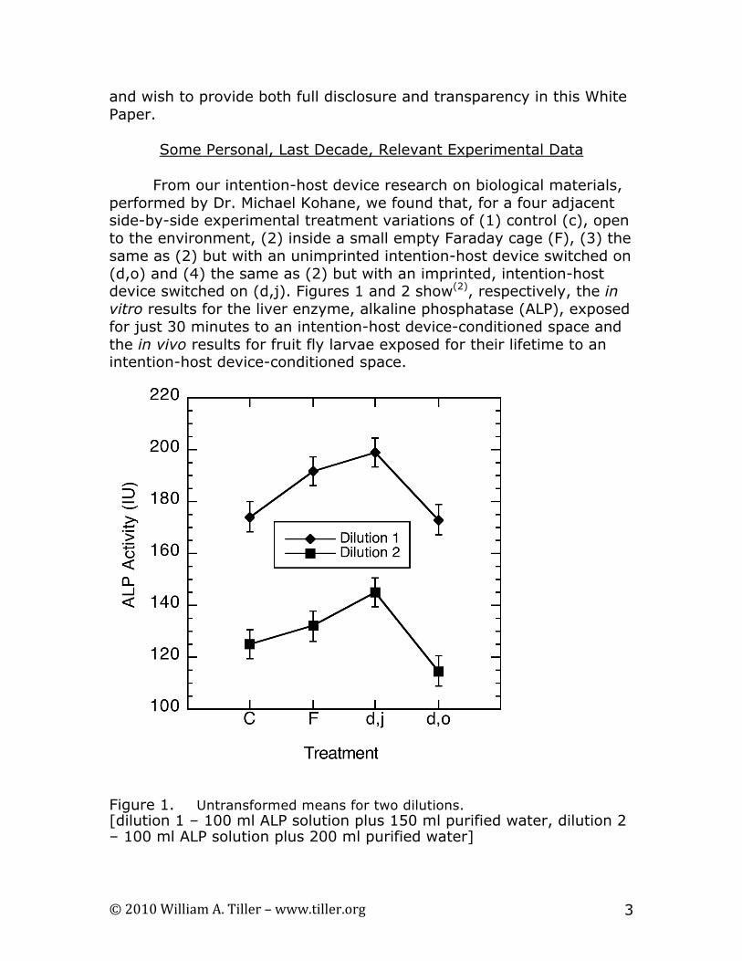
Some Personal, Last Decade, Relevant Experimental Data From our intention-host device research on biological materials, performed by Dr. Michael Kohane, we found that, for a four adjacent side-by-side experimental treatment variations of (1) control (c), open to the environment, (2) inside a small empty Faraday cage (F), (3) the same as (2) but with an unimprinted intention-host device switched on (d,o) and (4) the same as (2) but with an imprinted, intention-host device switched on (d,j). Figures 1 and 2 show(2), respectively, the in vitro results for the liver enzyme, alkaline phosphatase (ALP), exposed for just 30 minutes to an intention-host device-conditioned space and the in vivo results for fruit fly larvae exposed for their lifetime to an intention-host device-conditioned space.

Figure 1. Untransformed means for two dilutions. [dilution 1 – 100 ml ALP solution plus 150 ml purified water, dilution 2 – 100 ml ALP solution plus 200 ml purified water]


In Figure 1, the chemical activity of ALP is plotted versus the treatment for two dilutions of ALP in water. The key point, here, is to note that when, c, is removed from the ambient electromagnetic radiation and placed inside, F, the chemical activity of ALP (dilution 1) increased by ~7.5% at p<0.001. Thus, ambient EM radiation is a significant thermodynamic stressor for ALP. The electrical output power for the intention-host device is less than one millionth of a watt, all of it in the 1-10 megahertz range, and just a 30 minute exposure of the ALP inside F of this very low power, 10 MHz, EM radiation is sufficient to reduce the chemical activity of ALP by ~7.5% at p<0.001 (a very significant thermodynamic stressor for ALP). However, comparing the (d,j) result to the (d,o) result with the same EM radiation but with a specific imbedded intention to increase the ALP chemical activity, one sees that the αeff(t)(Qm+ΔQm) contribution to Equation 1 overcomes the effect of the EM radiation on ALP to yield a net increase of ALP activity by ~12.5% at p<0.001.

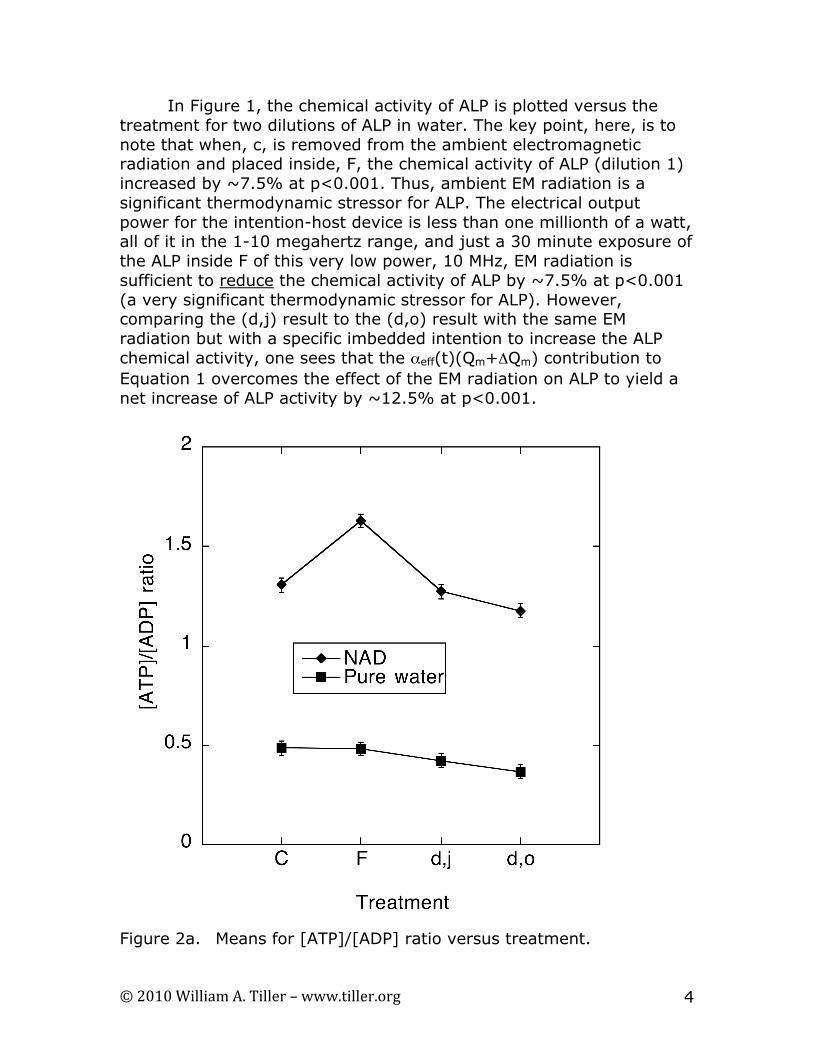
Figure 2a. Means for [ATP]/[ADP] ratio versus treatment.


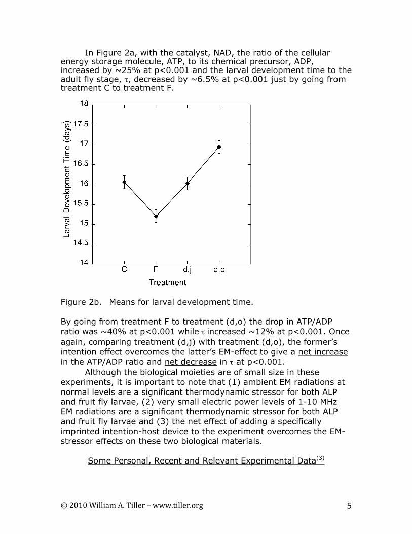
In Figure 2a, with the catalyst, NAD, the ratio of the cellular energy storage molecule, ATP, to its chemical precursor, ADP, increased by ~25% at p<0.001 and the larval development time to the adult fly stage, τ, decreased by ~6.5% at p<0.001 just by going from treatment C to treatment F.

Figure 2b. Means for larval development time. By going from treatment F to treatment (d,o) the drop in ATP/ADP ratio was ~40% at p<0.001 while τ increased ~12% at p<0.001. Once again, comparing treatment (d,j) with treatment (d,o), the former’s intention effect overcomes the latter’s EM-effect to give a net increase in the ATP/ADP ratio and net decrease in τ at p<0.001. Although the biological moieties are of small size in these experiments, it is important to note that (1) ambient EM radiations at normal levels are a significant thermodynamic stressor for both ALP and fruit fly larvae, (2) very small electric power levels of 1-10 MHz EM radiations are a significant thermodynamic stressor for both ALP and fruit fly larvae and (3) the net effect of adding a specifically imprinted intention-host device to the experiment overcomes the EM-stressor effects on these two biological materials.

Some Personal, Recent and Relevant Experimental Data(3)


A. Can experiments be done with IHD technology to directly show that, with biological materials and living systems, one can significantly reduce the magnitude of the EM-challenge from cell-phones? In general, I think that the answer is yes! However, it is an expensive procedure and such experimental work could not be undertaken until sufficient research funds were available. Here is how one might experimentally pursue such a goal:

• Ultimately, one wishes to measure the absorption cross-section, σ, of a human to the EM radiation from an activated cell-phone.

• We know that, with the proper receiving antenna equipment, one can quantitatively measure the EM-radiation spectrum intensity, I(r, θ, φ) as a function of distance, r, and orientation, (θ, φ), from a radiation source like an activated cell-phone.

• We also know that, if one places a layer of specific material of thickness, l, in the path of such an EM-source, some of this radiation intensity, ΔI, will be absorbed by this material. Assuming a negligible reflection coefficient of the EM radiation, the absorption coefficient, αA, is given by αA ~ΔI/l.

• By imprinting a specific intention to significantly reduce the magnitude of αA from cell phones, one could experimentally determine the efficacy of this particular process by determining ΔαA both before and after this intention had been introduced into the IHD used in the overall experiment.

This approach is much too expensive for us to contemplate at this time. However, the following series of steps is a possible pathway that is doable within the territory of our present resources.

Step 1; Create a strongly IHD-conditioned experimental space

(δGH+* ~ 20 meV)(1) with the appropriate intention. Step 2; Place a number of suitably-designed “talisman transfer

tokens” (TTT) into this coupled state experimental space for a period of time, τ, and record the time-dependent change in δGH+* for that space. This indicates a measure


of the “coupling substance”(2) transferred to each transfer token from the coupled state space.

Step 3; Place these treated “TTT” into an uncoupled state space

and measure the time-dependent change in the magnitude of δGH+* for this, now, partially coupled state space. This indicates a measure of the leakage rate of the coupling substance from the TTT to a normal, uncoupled state space.

Step 4; Adhesively attach one of the activated transfer tokens to

an uncoupled state cell phone in order to condition it to the partially coupled state with the specified intention.

Step 5; Because there is some leakage rate of coupling substance

from these TTTs into our normal environmental space, they have a finite effective lifetime and therefore should be replaced periodically (~ 3 months). When sufficient research funds have been gathered via royalties earned from the sale of these TTTs, the WAT Institute of Psychoenergetic Science will initiate experimental research, to “continuously” reimprint these TTTs via a long range information entanglement process(3).

References

1. William A. Tiller, “Psychoenergetic Science: A Second

Copernican-Scale Revolution”, Walnut Creek, CA, USA: Pavior Publishing, 2007.

2. William A. Tiller, Walter E. Dibble, Jr. and Michael J. Kohane,

“Conscious Acts of Creation”, Walnut Creek, CA, USA: Pavior Publishing, 2001.

3. William A. Tiller, “Psychoenergetic Science: A Second

Copernican-Scale Revolution”, Chapter 8, Walnut Creek, CA, USA: Pavior Publishing, 2007.

An On-going Experimental Study

Two, 12 cubic foot, wooden boxes (3.5 feet by 2.5 feet by 2 feet outer dimensions) were constructed and delivered to the laboratory on October 1, 2009. One conditioning box was placed in the lower shed of the property and the other was placed 125 feet away in a room of a


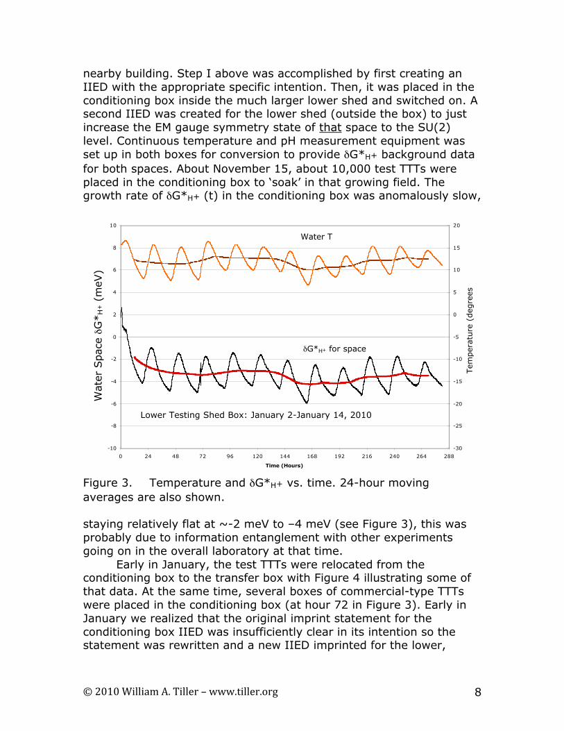
nearby building. Step I above was accomplished by first creating an IIED with the appropriate specific intention. Then, it was placed in the conditioning box inside the much larger lower shed and switched on. A second IIED was created for the lower shed (outside the box) to just increase the EM gauge symmetry state of that space to the SU(2) level. Continuous temperature and pH measurement equipment was set up in both boxes for conversion to provide δG*H+ background data for both spaces. About November 15, about 10,000 test TTTs were placed in the conditioning box to ‘soak’ in that growing field. The growth rate of δG*H+ (t) in the conditioning box was anomalously slow,

Figure 3. Temperature and δG*H+ vs. time. 24-hour moving averages are also shown. staying relatively flat at ~-2 meV to –4 meV (see Figure 3), this was probably due to information entanglement with other experiments going on in the overall laboratory at that time. Early in January, the test TTTs were relocated from the conditioning box to the transfer box with Figure 4 illustrating some of that data. At the same time, several boxes of commercial-type TTTs were placed in the conditioning box (at hour 72 in Figure 3). Early in January we realized that the original imprint statement for the conditioning box IIED was insufficiently clear in its intention so the statement was rewritten and a new IIED imprinted for the lower,

-10

-8

-6

-4

-2

0

2

4

6

8

10

0 24 48 72 96 120 144 168 192 216 240 264 288

Time (Hours)

Wat

er S

pace

!G

* H+ (

meV

)

-30

-25

-20

-15

-10

-5

0

5

10

15

20

Tem

pera

ture

(de

gree

s

Lower Testing Shed Box: January 2-January 14, 2010

Water T

!G*H+ for space


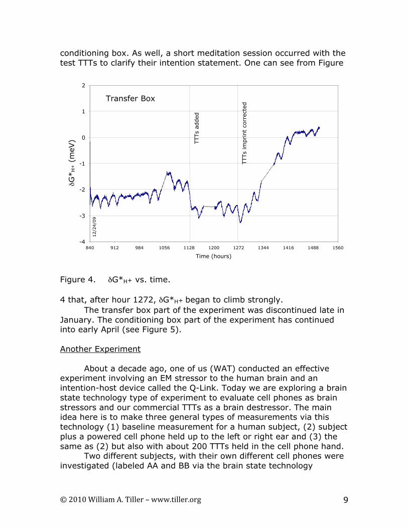
conditioning box. As well, a short meditation session occurred with the test TTTs to clarify their intention statement. One can see from Figure

Figure 4. δG*H+ vs. time. 4 that, after hour 1272, δG*H+ began to climb strongly. The transfer box part of the experiment was discontinued late in January. The conditioning box part of the experiment has continued into early April (see Figure 5). Another Experiment About a decade ago, one of us (WAT) conducted an effective experiment involving an EM stressor to the human brain and an intention-host device called the Q-Link. Today we are exploring a brain state technology type of experiment to evaluate cell phones as brain stressors and our commercial TTTs as a brain destressor. The main idea here is to make three general types of measurements via this technology (1) baseline measurement for a human subject, (2) subject plus a powered cell phone held up to the left or right ear and (3) the same as (2) but also with about 200 TTTs held in the cell phone hand. Two different subjects, with their own different cell phones were investigated (labeled AA and BB via the brain state technology

-4

-3

-2

-1

0

1

2

840 912 984 1056 1128 1200 1272 1344 1416 1488 1560

Time (hours)

! G* H

+ (

meV

) TTTs

add

ed

TTTs

impr

int

corr

ecte

d

12/2

4/09

Transfer Box


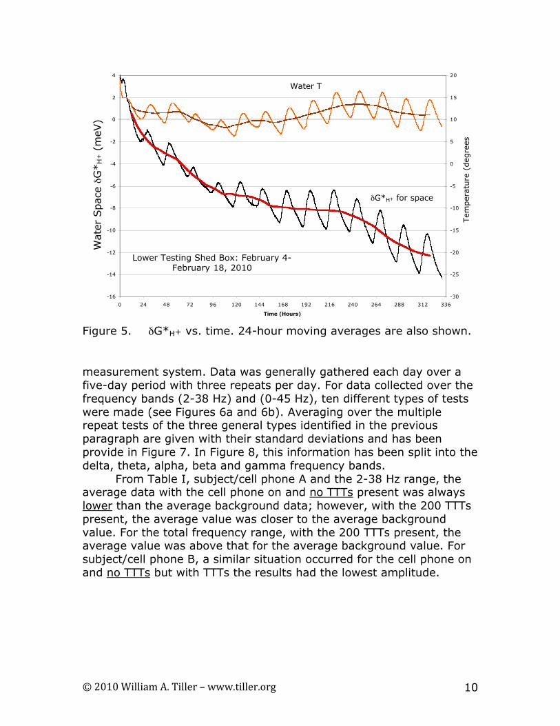
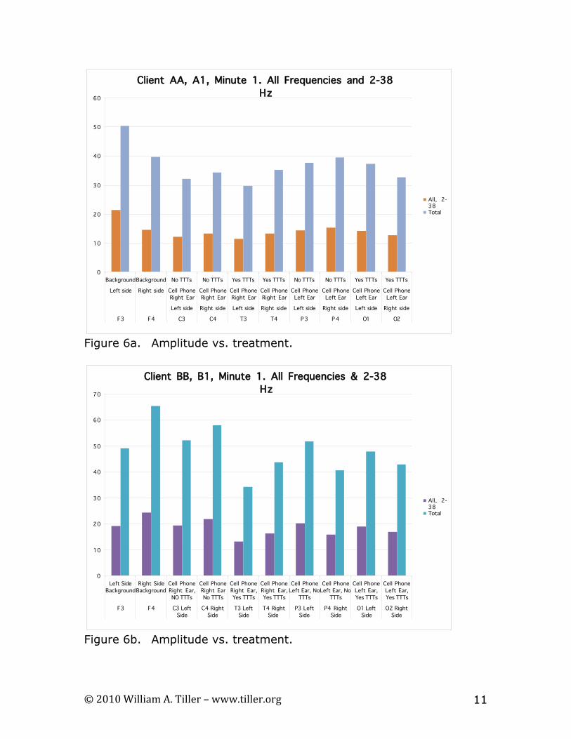
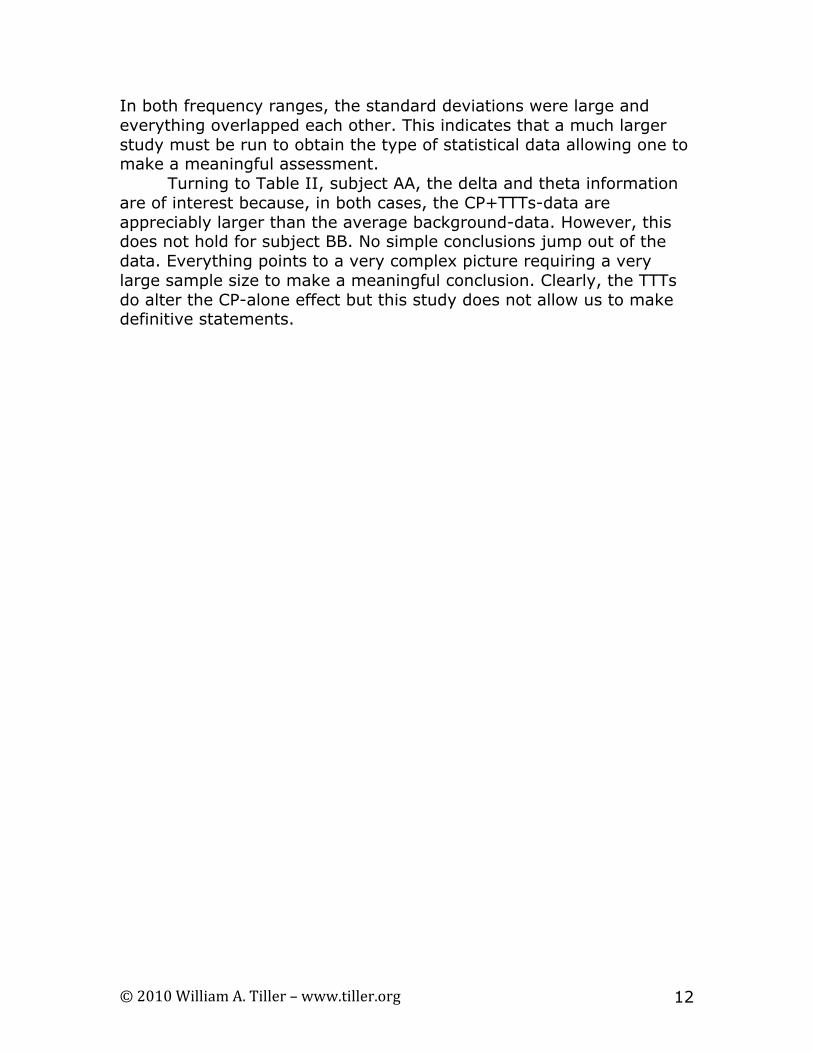
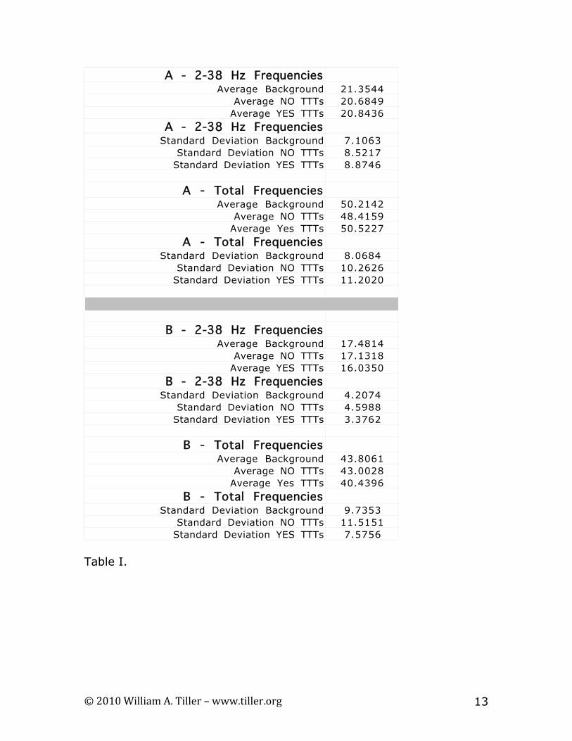
Figure 5. δG*H+ vs. time. 24-hour moving averages are also shown. measurement system. Data was generally gathered each day over a five-day period with three repeats per day. For data collected over the frequency bands (2-38 Hz) and (0-45 Hz), ten different types of tests were made (see Figures 6a and 6b). Averaging over the multiple repeat tests of the three general types identified in the previous paragraph are given with their standard deviations and has been provide in Figure 7. In Figure 8, this information has been split into the delta, theta, alpha, beta and gamma frequency bands. From Table I, subject/cell phone A and the 2-38 Hz range, the average data with the cell phone on and no TTTs present was always lower than the average background data; however, with the 200 TTTs present, the average value was closer to the average background value. For the total frequency range, with the 200 TTTs present, the average value was above that for the average background value. For subject/cell phone B, a similar situation occurred for the cell phone on and no TTTs but with TTTs the results had the lowest amplitude.

-16

-14

-12

-10

-8

-6

-4

-2

0

2

4

0 24 48 72 96 120 144 168 192 216 240 264 288 312 336

Time (Hours)

Wat

er S

pace

!G

* H+ (

meV

)

-30

-25

-20

-15

-10

-5

0

5

10

15

20

Tem

pera

ture

(de

gree

s

Lower Testing Shed Box: February 4-February 18, 2010

Water T

!G*H+ for space


Figure 6a. Amplitude vs. treatment.

Figure 6b. Amplitude vs. treatment.

Client AA, A1, Minute 1. All Frequencies and 2-38 Hz

0

10

20

30

40

50

60

BackgroundBackground No TTTs No TTTs Yes TTTs Yes TTTs No TTTs No TTTs Yes TTTs Yes TTTs

Left side Right side Cell PhoneRight Ear

Cell PhoneRight Ear

Cell PhoneRight Ear

Cell PhoneRight Ear

Cell PhoneLeft Ear

Cell PhoneLeft Ear

Cell PhoneLeft Ear

Cell PhoneLeft Ear

Left side Right side Left side Right side Left side Right side Left side Right side

F3 F4 C3 C4 T3 T4 P3 P4 O1 O2

All, 2-38Total

Client BB, B1, Minute 1. All Frequencies & 2-38 Hz

0

10

20

30

40

50

60

70

Left SideBackground

Right SideBackground

Cell PhoneRight Ear,NO TTTs

Cell PhoneRight EarNo TTTs

Cell PhoneRight Ear,Yes TTTs

Cell PhoneRight Ear,Yes TTTs

Cell PhoneLeft Ear, No

TTTs

Cell PhoneLeft Ear, No

TTTs

Cell PhoneLeft Ear,Yes TTTs

Cell PhoneLeft Ear,Yes TTTs

F3 F4 C3 LeftSide

C4 RightSide

T3 LeftSide

T4 RightSide

P3 LeftSide

P4 RightSide

O1 LeftSide

O2 RightSide

All, 2-38Total


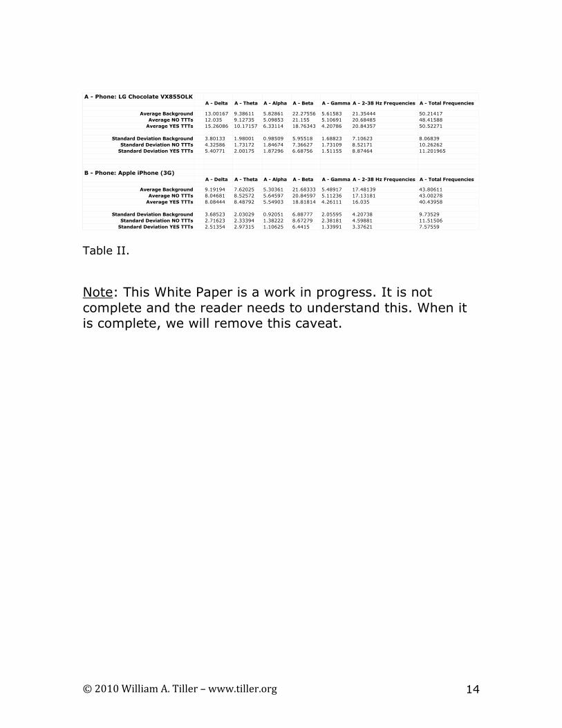
In both frequency ranges, the standard deviations were large and everything overlapped each other. This indicates that a much larger study must be run to obtain the type of statistical data allowing one to make a meaningful assessment. Turning to Table II, subject AA, the delta and theta information are of interest because, in both cases, the CP+TTTs-data are appreciably larger than the average background-data. However, this does not hold for subject BB. No simple conclusions jump out of the data. Everything points to a very complex picture requiring a very large sample size to make a meaningful conclusion. Clearly, the TTTs do alter the CP-alone effect but this study does not allow us to make definitive statements.


Table I.

A - 2-38 Hz FrequenciesAverage Background 21.3544

Average NO TTTs 20.6849Average YES TTTs 20.8436

A - 2-38 Hz FrequenciesStandard Deviation Background 7.1063

Standard Deviation NO TTTs 8.5217Standard Deviation YES TTTs 8.8746

A - Total FrequenciesAverage Background 50.2142

Average NO TTTs 48.4159Average Yes TTTs 50.5227

A - Total FrequenciesStandard Deviation Background 8.0684


B - 2-38 Hz FrequenciesAverage Background 17.4814

Average NO TTTs 17.1318Average YES TTTs 16.0350

B - 2-38 Hz FrequenciesStandard Deviation Background 4.2074


B - Total FrequenciesAverage Background 43.8061

Average NO TTTs 43.0028Average Yes TTTs 40.4396

B - Total FrequenciesStandard Deviation Background 9.7353



Table II. Note: This White Paper is a work in progress. It is not complete and the reader needs to understand this. When it is complete, we will remove this caveat.

A - Phone: LG Chocolate VX855OLKA - Delta A - Theta A - Alpha A - Beta A - Gamma A - 2-38 Hz Frequencies A - Total Frequencies

Average Background 13.00167 9.38611 5.82861 22.27556 5.61583 21.35444 50.21417Average NO TTTs 12.035 9.12735 5.09853 21.155 5.10691 20.68485 48.41588

Average YES TTTs 15.26086 10.17157 6.33114 18.76343 4.20786 20.84357 50.52271

Standard Deviation Background 3.80133 1.98001 0.98509 5.95518 1.68823 7.10623 8.06839Standard Deviation NO TTTs 4.32586 1.73172 1.84674 7.36627 1.73109 8.52171 10.26262

Standard Deviation YES TTTs 5.40771 2.00175 1.87296 6.68756 1.51155 8.87464 11.201965

B - Phone: Apple iPhone (3G)A - Delta A - Theta A - Alpha A - Beta A - Gamma A - 2-38 Hz Frequencies A - Total Frequencies

Average Background 9.19194 7.62025 5.30361 21.68333 5.48917 17.48139 43.80611Average NO TTTs 8.04681 8.52572 5.64597 20.84597 5.11236 17.13181 43.00278

Average YES TTTs 8.08444 8.48792 5.54903 18.81814 4.26111 16.035 40.43958

Standard Deviation Background 3.68523 2.03029 0.92051 6.88777 2.05595 4.20738 9.73529Standard Deviation NO TTTs 2.71623 2.33394 1.38222 8.67279 2.38181 4.59881 11.51506

Standard Deviation YES TTTs 2.51354 2.97315 1.10625 6.4415 1.33991 3.37621 7.57559

Documents

White Paper XIV