White-light channeled imaging polarimeter using broadband ... · White-light channeled imaging polarimeter using broadband polarization gratings Michael W. Kudenov,1,* Michael J

White-light channeled imaging polarimeter usingbroadband polarization gratings

Michael W. Kudenov,1,* Michael J. Escuti,2 Eustace L. Dereniak,1 and Kazuhiko Oka3

1College of Optical Science, The University of Arizona, 1630 E. University Boulevard, Tucson, Arizona 85721, USA2Department of Electrical and Computer Engineering, North Carolina State University,

2410 Campus Shore Drive, Raleigh, North Carolina 27606, USA3Division of Applied Physics, Hokkaido University, N-13, W-8, Sapporo 060-8628, Japan

*Corresponding author: [email protected]

Received 30 November 2010; revised 2 March 2011; accepted 7 March 2011;posted 9 March 2011 (Doc. ID 138651); published 18 May 2011

A white-light snapshot channeled linear imaging (CLI) polarimeter is demonstrated by utilizing polar-ization gratings (PGs). The CLI polarimeter is capable of measuring the two-dimensional distribution ofthe linear Stokes polarization parameters by incorporating two identical PGs, in series, along the opticalaxis. In this configuration, the general optical shearing functionality of a uniaxial crystal-based Savartplate is realized. However, unlike a Savart plate, the diffractive nature of the PGs creates a linear de-pendence of the shear versus wavelength, thus providing broadband functionality. Consequently, by in-corporating the PG-based Savart plate into a Savart plate channeled imaging polarimeter, white-lightinterference fringes can be generated. This enables polarimetric image data to be acquired at shorterexposure times in daylight conditions, making it more appealing over the quasi-monochromatic chan-neled imaging polarimeters previously described in the literature. Furthermore, the PG-based deviceoffers significantly more compactness, field of view, optical simplicity, and vibration insensitivity thanpreviously described white-light CLI polarimeters based on Sagnac interferometers. Included in this pa-per are theoretical descriptions of the linear (S0, S1, and S2) and complete (S0, S1, S2, and S3) channeledStokes imaging polarimeters. Additionally, descriptions of our calibration procedures and our experimen-tal proof of concept CLI system are provided. These are followed by laboratory and outdoor polarimetricmeasurements of S0, S1, and S2. © 2011 Optical Society of AmericaOCIS codes: 110.3175, 300.6190, 110.5405.

1. Introduction

Imaging polarimetry is used to measure the two-dimensional (2D) spatial Stokes parameter dis-tribution of a scene. It is a valuable tool in thecharacterization of aerosol size distributions, distin-guishing man-made targets from background clutter,quality control for evaluating the distribution ofstress birefringence, and for evaluating biological tis-sues in medical imaging [1,2]. The Stokes vector isdefined as

Sðx; yÞ ¼

264S0ðx; yÞS1ðx; yÞS2ðx; yÞS3ðx; yÞ

375 ¼

264

I0ðx; yÞ þ I90ðx; yÞI0ðx; yÞ − I90ðx; yÞI45ðx; yÞ − I135ðx; yÞIRðx; yÞ − ILðx; yÞ

375; ð1Þ

where x, y are spatial coordinates in the scene, S0 isthe total power of the beam, S1 denotes preference forlinear 0° over 90°, S2 for linear 45° over 135°, and S3for right circular over left circular polarizationstates. By measuring all four elements of Sðx; yÞ,the complete spatial distribution of the polarizationstate can be determined.

Typically, Stokes parameters are measured byrecording four intensity measurements sequen-tially using different configurations of polarization

0003-6935/11/152283-11$15.00/0© 2011 Optical Society of America

20 May 2011 / Vol. 50, No. 15 / APPLIED OPTICS 2283

analyzers. By utilizing the instrument’s polarimetricresponse, all Stokes parameters can be calculatedby using Mueller matrix calculus. However, time-sequentialmeasurements of a rapidly changing sceneare susceptible to temporal misregistration. For in-stance, any motion-induced intensity variations thatoccur between the time-sequential measurementswill appear as a false depolarization signature.There-fore, in order to avoid temporal registration error, allintensitymeasurementsmust be recorded in parallel.There are several instruments that canmeasure com-plete Stokes vectors or individual Stokes parameterswithin a single snapshot of a camera(s). These includedivision of focal plane (DoFP), division of amplitude(DoAM), division of aperture (DoA), and channeledimaging polarimeters (CIPs) [1].

Here, we focus on CIPs [3–5]. In a CIP, interferome-trically generated carrier frequencies are amplitudemodulated with the spatially dependent 2D Stokesparameters. Two advantages of a CIP, over the pre-viously listed polarimeters (DoFP, DoAM, and DoA),include its inherent image registration and simple op-tical implementation. Namely, image registration isinherent since all the Stokes parameters are directlymodulated onto coincident interference fringes.Additionally, the optical instrumentation requiredto incorporate CIP can be augmented onto nearlyany pre-existing lens and camera system with mini-mal effort.

In this paper, we present an instrumentation im-provement for CIP. Specifically, we demonstrate asignificantly more compact version of our white-lightCIP, originally based on a modified Sagnac interfe-rometer [6,7] or an achromatic Fourier transforminglens [8]. By incorporating polarization gratings (PGs)as a diffractive Savart plate, the functional form ofthe Sagnac interferometer’s white-light fringesare preserved [9]. In Section 2, we outline the theo-retical basis of the white-light channeled linearimaging (CLI) polarimeter with polarization grat-ings. Section 3 describes the calibration procedurefor the CLI polarimeter, followed by an experimentalverification and validation of the system in Section 4.Section 4 also includes details of our outdoor testing.Finally, Appendix A theoretically describes the re-quired system modifications to measure a completeStokes vector in white light.

2. Channeled Imaging Polarimetry UsingPolarization Gratings

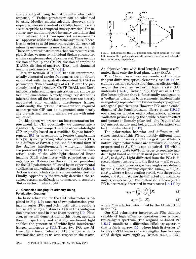
The basic schematic for the CLI polarimeter is de-picted in Fig. 1. It consists of two polarization grat-ings in series (PG1 and PG2), both with a period Λand separated by a distance t. PGs in this configura-tion have been used in laser beam steering [10]. How-ever, as we will demonstrate in this paper, applyingthem in spectrally and spatially incoherent lightenables the generation of white-light interferencefringes, analogous to [11]. These two PGs are fol-lowed by a linear polarizer (LP) oriented with itstransmission axis at 0° with respect to the x axis.

An objective lens, with focal length f , images colli-mated light onto the focal plane array (FPA).

The PGs employed here are members of the bire-fringent diffractive optical elements class [12–14] in-cluding spatially periodic birefringence effects, whichare, in this case, realized using liquid crystal (LC)materials [14–18]. Individually, they act as a thin-film beam splitter that is functionally analogous toa Wollaston prism. In both elements, incident lightis angularly separated into two forward-propagating,orthogonal polarizations. However, PGs are an embo-diment of the Pancharatnam-–Berry phase [19,20]operating on circular eigen-polarizations, whereasWollaston prisms employ the double refraction effectand operate on linearly polarized light. Details of theLC microstructure and holographic fabrication canbe found elsewhere [16,17].

The polarization behavior and diffraction effi-ciency spectra of this PG are notably different thanconventional phase or amplitude gratings. While itsnatural eigen-polarizations are circular (i.e., linearlyproportional to S3=S0), it can be paired [17] with aquarter-wave plate (QWP) in order to separate inci-dent light based on other desired polarizations (i.e.,S1=S0 or S2=S0). Light diffracted from the PGs is di-rected almost entirely into the first (m ¼ �1) or zero(m ¼ 0) diffraction orders, where angles are definedby the classical grating equation (sin θm ¼ mλ=Λ−

sin θin, whereΛ is the grating period,m is the gratingorder, and θm and θin are the diffracted and incidenceangles, respectively). The diffraction efficiency of aPG is accurately described in most cases [14,17] by

η�1 ¼�12∓

S3

2S0

�K ; ð2Þ

η0 ¼ ð1 − KÞ; ð3Þwhere K is a factor determined by the LC structurein the PG.

Our CLI polarimeter incorporates PGs that arecapable of high efficiency operation over a broad(white-light) spectrum. The original LC-based PG[16,17] manifests a diffraction efficiency spectrumthat is fairly narrow [15], where high first-order ef-ficiency (>99%) occurs at wavelengths close to a spe-cified design wavelength λ0 (within Δλ=λ0 ∼ 13%).

Fig. 1. Schematic of the CLI polarimeter. Right circular (RC) andleft circular (LC) polarizations diffract into the −1st and þ1st dif-fraction orders, respectively.

2284 APPLIED OPTICS / Vol. 50, No. 15 / 20 May 2011

Through optimization and refinement of the diffrac-tive structure, a broadband PG [15] enables a largerhigh efficiency spectral bandwidth (Δλ=λ0 ∼ 56%),which can cover most of the visible wavelengthrange. In this case, a good approximation is K ¼ 1,so that η�1 ¼ 1 and η0 ¼ 0 for most visible wave-lengths (e.g., 450–750nm).

In our CLI polarimeter, incident light is trans-mitted by PG1 and initially diffracted into its leftand right circularly polarized components, propagat-ing above and below the optical axis, respectively.After transmission through PG2, the two beams(EA and EB) are diffracted again to propagate parallelto the optical axis and are now sheared by a distanceα. The linear polarizer analyzes both beams, thusunifying the polarization state. Imaging both beamsonto the FPA combines the two beams and producesinterference fringes. To calculate the intensity pat-

tern on the FPA, assume an arbitrarily polarizedelectric field is incident on the first polarization grat-ing (PG1). The incident field can be expressed as

Einc ¼��EX�EY

�¼

�EXðξ; ηÞejφxðξ;ηÞ

EYðξ; ηÞejφyðξ;ηÞ

�; ð4Þ

where ξ, η are the angular spectrum components of xand y, respectively. The PG’s þ1st and −1st diffrac-tion orders can be modeled as right and left circularpolarization analyzers with their Jones matricesexpressed as

Jþ1;RC ¼ 12

�1 i−i 1

�; ð5Þ

J−1;LC ¼ 12

�1 −ii 1

�: ð6Þ

After transmission through PG1 and PG2, the x and ypolarization components of the electric field, for eachof the two beams, are

EA ¼ J−1;LCEinc ¼12

��EXðξ; η − αÞ − j�EYðξ; η − αÞj�EXðξ; η − αÞ þ �EYðξ; η − αÞ

�;

ð7Þ

EB ¼ Jþ1;RCEinc ¼12

��EXðξ; ηþ αÞ þ j�EYðξ; ηþ αÞ−j�EXðξ; ηþ αÞ þ �EYðξ; ηþ αÞ

�;

ð8Þ

where α is the shear, calculated using the paraxialapproximation as

α ≅mλΛ t; ð9Þ

and m is the diffraction order (being either 1 or −1).The total electric field incident on the linear polari-zer (LP) is

EþLP ¼ EA þ EB ¼ 1

2

��EXðξ; ηþ αÞ þ j�EYðξ; ηþ αÞ þ �EXðξ; η − αÞ − j�EYðξ; η − αÞ−j�EXðξ; ηþ αÞ þ �EYðξ; ηþ αÞ þ j�EXðξ; η − αÞ þ �EYðξ; η − αÞ

�: ð10Þ

Transmission through the linear polarizer, with itstransmission axis at 0°, yields

E−

LP ¼�1 00 0

�EþLP ¼ 1

2

��EXðξ; ηþ αÞ þ j�EYðξ; ηþ αÞ þ �EXðξ; η − αÞ − j�EYðξ; η − αÞ

0

�: ð11Þ

The objective lens produces a Fourier transformationof the field as

Ef ¼ F½E−

LP�ξ¼ xλf ;η¼ y

λf

¼ 12

��EXe

j2πλf αy þ j�EYej2πλf αy þ �EXe

−j2πλf αy − j�EYe−j2πλf αy

�;

ð12Þ

where �EX and �EY are now implicitly dependent uponx and y and f is the focal length of the objective lens.Total electric field intensity can be written as follows:

I ¼ jEf j2

¼ 12ðj�EX j2 þ j�EY j2Þ þ

14ð�EX

�E�X − �EY

�E�YÞej

2πλf 2αy

þ 14ð�EX

�E�X − �EY

�E�YÞe−j

2πλf 2αy

þ j14ð�EX

�E�Y þ �EY

�E�XÞej

2πλf 2αy

− j14ð�EX

�E�Y þ �EY

�E�XÞe−j

2πλf 2αy: ð13Þ

Simplification using the Stokes parameter defini-tions [21] yields the final expression for the intensitypattern:


Iðx; yÞ ¼ 12

�S0ðx; yÞ þ S1ðx; yÞ cos

�2πλf 2αy

�

þ S2ðx; yÞ sin�2πλf 2αy

��: ð14Þ

Consequently, the intensity recorded on the FPA con-tains the amplitude modulated Stokes parametersS0, S1, and S2. Substitution of the shear intoEq. (14) produces

Iðx; yÞ ¼ 12

�S0ðx; yÞ þ S1ðx; yÞ cos

�2π 2mt

fΛ y

�

þ S2ðx; yÞ sin�2π 2mt

fΛ y

��: ð15Þ

From the Eq. (15), the frequency of the interferencefringe, or the carrier frequency, denoted by U, is

U ¼ 2mtfΛ : ð16Þ

Thus, the linear Stokes parameters are amplitudemodulated onto spectrally broadband (white-light)interference fringes. Extending this technique tofull Stokes imaging polarimetry is detailed inAppendix A. However, our calibration techniqueand experimental demonstration focuses on the lin-ear polarimeter due to PG availability.

3. CLI Polarimeter Calibration

The CLI polarimeter is calibrated by applying the re-ference beam calibration technique [4,8]. First, a for-

ward 2D Fourier transformation is performed on theintensity pattern of Eq. (15), producing

Iðξ;ηÞ¼F½Iðx;yÞ�

¼ 12S0ðξ;ηÞþ

14S1ðξ;ηÞ � ½δðξ;ηþUÞþδðξ;η−UÞ�

þ i14S2ðξ;ηÞ � ½δðξ;ηþUÞ−δðξ;η−UÞ�; ð17Þ

where ξ and η are the Fourier transform variables forx and y, respectively, and δ is the Dirac delta function.Equation (17) indicates the presence of three “chan-nels” in the Fourier domain. The S1 and S2 Stokes

parameters are modulated (i.e., convolved) by twoshifted (�U) delta functions, while the S0 Stokesparameter remains unmodulated. These three chan-nelsaredenotedasC0 (S0),C1 (ðS1 − iS2Þ � δðξ; η −UÞ),and C�

1 (ðS1 þ iS2Þ � δðξ; ηþUÞ). Applying a 2D filterto two of the three channels (C0 andC1 orC�

1), followedby an inverse Fourier transformation, enables theircontent to be isolated from the other components. In-verse Fourier transformation of channels C0 and C1produces

C0 ¼ 12S0ðx; yÞ; ð18Þ

C1 ¼ 14ðS1ðx; yÞ − iS2ðx; yÞÞei2πUy: ð19Þ

Therefore, the S0 Stokes parameter can be extracteddirectly fromEq. (18),while theS1 andS2 componentsare modulated by an exponential phase factor ei2πUy.Isolating this phase factor from the sample data(C0;sample and C1;sample) is accomplished by comparingit to a previously measured reference polarizationstate (C0;ref andC1;ref ) containing the known distribu-tion ½S0;ref ;S1;ref ;S2;ref ;S3;ref �T . The sample’s Stokesparameters are demodulated by dividing the sampledata by the reference data, followed by normalizationto the S0 Stokes parameter and extraction of the realand imaginary parts:

S0ðx; yÞ ¼ jC0;samplej; ð20Þ

S1ðx; yÞS0ðx; yÞ

¼ R

�C1;sample

C1;reference

C0;reference

C0;sample

�S1;ref ðx; yÞ − iS2;ref ðx; yÞ

S0;ref ðx; yÞ��

; ð21Þ


¼ I

�C1;sample

C1;reference

C0;reference

C0;sample

�S1;ref ðx; yÞ − iS2;ref ðx; yÞ

S0;ref ðx; yÞ��

: ð22Þ

For instance, using reference data created by a linearpolarizer, oriented at 0° ½S0;S1;S2;S3�T ¼ ½1; 1; 0; 0�T ,yields the following reference-beam calibrationequations:

S0ðx; yÞ ¼ jC0;samplej; ð23Þ


¼ R

�C1;sample

C1;reference

C0;reference

C0;sample

�; ð24Þ


¼ I

�C1;sample

C1;reference

C0;reference

C0;sample

�: ð25Þ


Equations (23)–(25) are applied to themeasured datain order to extract the scene’s spatially dependentStokes parameters.

4. Experimental Verification of the CLI Polarimeter

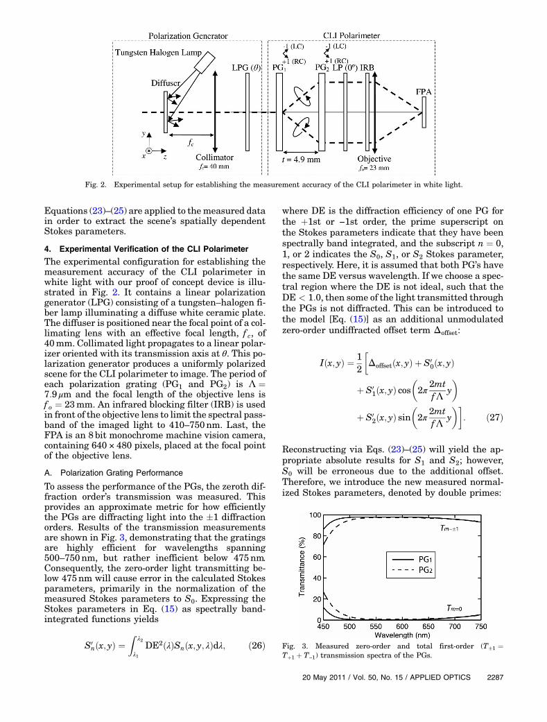
The experimental configuration for establishing themeasurement accuracy of the CLI polarimeter inwhite light with our proof of concept device is illu-strated in Fig. 2. It contains a linear polarizationgenerator (LPG) consisting of a tungsten–halogen fi-ber lamp illuminating a diffuse white ceramic plate.The diffuser is positioned near the focal point of a col-limating lens with an effective focal length, f c, of40mm. Collimated light propagates to a linear polar-izer oriented with its transmission axis at θ. This po-larization generator produces a uniformly polarizedscene for the CLI polarimeter to image. The period ofeach polarization grating (PG1 and PG2) is Λ ¼7:9 μm and the focal length of the objective lens isf o ¼ 23mm. An infrared blocking filter (IRB) is usedin front of the objective lens to limit the spectral pass-band of the imaged light to 410–750nm. Last, theFPA is an 8 bit monochrome machine vision camera,containing 640 × 480 pixels, placed at the focal pointof the objective lens.

A. Polarization Grating Performance

To assess the performance of the PGs, the zeroth dif-fraction order’s transmission was measured. Thisprovides an approximate metric for how efficientlythe PGs are diffracting light into the �1 diffractionorders. Results of the transmission measurementsare shown in Fig. 3, demonstrating that the gratingsare highly efficient for wavelengths spanning500–750nm, but rather inefficient below 475nm.Consequently, the zero-order light transmitting be-low 475nm will cause error in the calculated Stokesparameters, primarily in the normalization of themeasured Stokes parameters to S0. Expressing theStokes parameters in Eq. (15) as spectrally band-integrated functions yields

S0nðx; yÞ ¼

Z λ2

λ1DE2ðλÞSnðx; y; λÞdλ; ð26Þ

where DE is the diffraction efficiency of one PG forthe þ1st or −1st order, the prime superscript onthe Stokes parameters indicate that they have beenspectrally band integrated, and the subscript n ¼ 0,1, or 2 indicates the S0, S1, or S2 Stokes parameter,respectively. Here, it is assumed that both PG’s havethe same DE versus wavelength. If we choose a spec-tral region where the DE is not ideal, such that theDE < 1:0, then some of the light transmitted throughthe PGs is not diffracted. This can be introduced tothe model [Eq. (15)] as an additional unmodulatedzero-order undiffracted offset term Δoffset:

Iðx; yÞ ¼ 12

�Δoffsetðx; yÞ þ S0

0ðx; yÞ

þ S01ðx; yÞ cos

�2π 2mt

fΛ y

�

þ S02ðx; yÞ sin

�2π 2mt

fΛ y

��: ð27Þ

Reconstructing via Eqs. (23)–(25) will yield the ap-propriate absolute results for S1 and S2; however,S0 will be erroneous due to the additional offset.Therefore, we introduce the new measured normal-ized Stokes parameters, denoted by double primes:

Fig. 2. Experimental setup for establishing the measurement accuracy of the CLI polarimeter in white light.

Fig. 3. Measured zero-order and total first-order (T�1 ¼Tþ1 þ T−1) transmission spectra of the PGs.


S000ðx; yÞ ¼ S0

0ðx; yÞ þΔoffsetðx; yÞ; ð28Þ

S00nðx; yÞ

S000ðx; yÞ

¼ S0nðx; yÞ

S00ðx; yÞ þΔoffsetðx; yÞ

; ð29Þ

where the subscript n ¼ 1 or 2 indicates the S1 or S2Stokes parameter, respectively. Consequently, erroris induced into the S1 and S2 Stokes parameters fromthe normalization to the effectively larger S0 compo-nent [S0

0ðx; yÞ þΔoffsetðx; yÞ]. While error due to thiszero-order light leakage was observed in our outdoortests, it was negligible in our laboratory characteri-zation because our S0 reference and sample illumina-tion levels were constant. Ultimately, we anticipatethat PGs with a zero-order light transmission ofless than 3% over the passband would enable betteraccuracy regardless of the S0 illumination level.For our proof of concept experiments, we aim atdemonstrating the CLI polarimeter’s ability to gen-erate white-light polarization-induced interferencefringes.

B. Calibration Verification

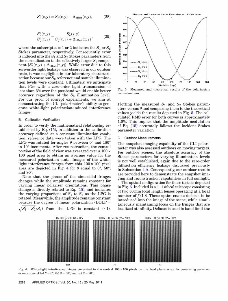
In order to verify the mathematical relationship es-tablished by Eq. (15), in addition to the calibrationaccuracy defined at a constant illumination condi-tion, reference data were taken with the LPG. TheLPG was rotated for angles θ between 0° and 180°in 10° increments. After reconstruction, the centralportion of the field of view was averaged over a 100 ×100 pixel area to obtain an average value for themeasured polarization state. Images of the white-light interference fringes from this 100 × 100 pixelarea are depicted in Fig. 4 for θ equal to 0°, 50°,and 90°.

Note that the phase of the sinusoidal fringeschanges while the amplitude remains constant forvarying linear polarizer orientations. This phasechange is directly related to Eq. (15), and indicatesthe varying proportions of S1 to S2 as the LPG isrotated. Meanwhile, the amplitude remains constantbecause the degree of linear polarization (DOLP ¼ffiffiffiffiffiffiffiffiffiffiffiffiffiffiffiffiffi

S21 þ S2

2

q=S0) from the LPG is constant (∼1).

Plotting the measured S1 and S2 Stokes param-eters versus θ and comparing them to the theoreticalvalues yields the results depicted in Fig. 5. The cal-culated RMS error for both curves is approximately1.6%. This implies that the amplitude modulationof Eq. (15) accurately follows the incident Stokesparameter variation.

C. Outdoor Measurements

The snapshot imaging capability of the CLI polari-meter was also assessed outdoors on moving targets.For outdoor scenes, the absolute accuracy of theStokes parameters for varying illumination levelsis not well established, again due to the zero-orderdiffraction efficiency leakage discussed previouslyin Subsection 4.A. Consequently, our outdoor resultsare provided here to demonstrate the snapshot ima-ging and reconstruction capabilities in full sunlight.

The optical configuration for these tests is depictedin Fig. 6. Included is a 1∶1 afocal telescope consistingof two 50mm focal length lenses operating at a focalnumber of f =1:8. These optics enable defocus to beintroduced into the image of the scene, while simul-taneously maintaining focus on the fringes that arelocalized at infinity. Defocus is used to band limit the

Fig. 4. White-light interference fringes generated in the central 100 × 100 pixels on the focal plane array for generating polarizerorientations of (a) θ ¼ 0°, (b) θ ¼ 50°, and (c) θ ¼ 90°.

Fig. 5. Measured and theoretical results of the polarimetricreconstructions.


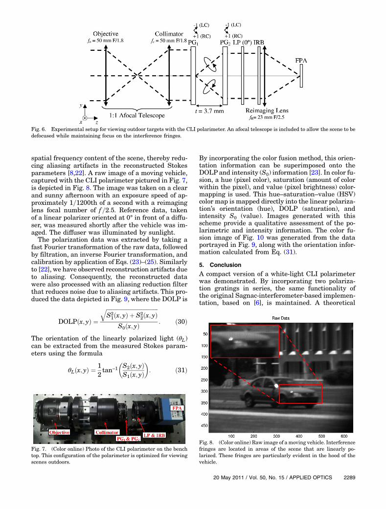
spatial frequency content of the scene, thereby redu-cing aliasing artifacts in the reconstructed Stokesparameters [8,22]. A raw image of a moving vehicle,captured with the CLI polarimeter pictured in Fig. 7,is depicted in Fig. 8. The image was taken on a clearand sunny afternoon with an exposure speed of ap-proximately 1=1200th of a second with a reimaginglens focal number of f =2:5. Reference data, takenof a linear polarizer oriented at 0° in front of a diffu-ser, was measured shortly after the vehicle was im-aged. The diffuser was illuminated by sunlight.

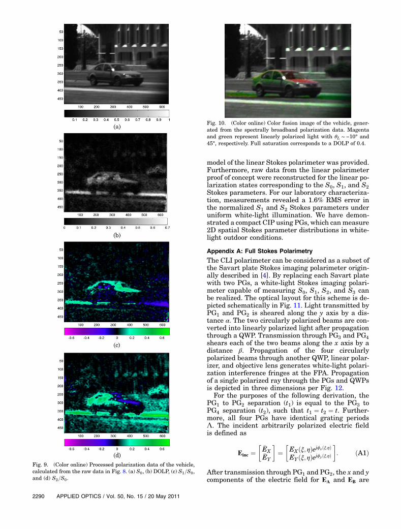
The polarization data was extracted by taking afast Fourier transformation of the raw data, followedby filtration, an inverse Fourier transformation, andcalibration by application of Eqs. (23)–(25). Similarlyto [22], we have observed reconstruction artifacts dueto aliasing. Consequently, the reconstructed datawere also processed with an aliasing reduction filterthat reduces noise due to aliasing artifacts. This pro-duced the data depicted in Fig. 9, where the DOLP is

DOLPðx; yÞ ¼ffiffiffiffiffiffiffiffiffiffiffiffiffiffiffiffiffiffiffiffiffiffiffiffiffiffiffiffiffiffiffiffiffiffiffiffiffiffiS21ðx; yÞ þ S2

2ðx; yÞq

S0ðx; yÞ: ð30Þ

The orientation of the linearly polarized light (θL)can be extracted from the measured Stokes param-eters using the formula

θLðx; yÞ ¼12tan−1

�S2ðx; yÞS1ðx; yÞ

�: ð31Þ

By incorporating the color fusion method, this orien-tation information can be superimposed onto theDOLPand intensity (S0) information [23]. In color fu-sion, a hue (pixel color), saturation (amount of colorwithin the pixel), and value (pixel brightness) color-mapping is used. This hue–saturation–value (HSV)color map is mapped directly into the linear polariza-tion’s orientation (hue), DOLP (saturation), andintensity S0 (value). Images generated with thisscheme provide a qualitative assessment of the po-larimetric and intensity information. The color fu-sion image of Fig. 10 was generated from the dataportrayed in Fig. 9, along with the orientation infor-mation calculated from Eq. (31).

5. Conclusion

A compact version of a white-light CLI polarimeterwas demonstrated. By incorporating two polariza-tion gratings in series, the same functionality ofthe original Sagnac-interferometer-based implemen-tation, based on [6], is maintained. A theoretical

Fig. 6. Experimental setup for viewing outdoor targets with the CLI polarimeter. An afocal telescope is included to allow the scene to bedefocused while maintaining focus on the interference fringes.

Fig. 7. (Color online) Photo of the CLI polarimeter on the benchtop. This configuration of the polarimeter is optimized for viewingscenes outdoors.

Fig. 8. (Color online) Raw image of a moving vehicle. Interferencefringes are located in areas of the scene that are linearly po-larized. These fringes are particularly evident in the hood of thevehicle.


model of the linear Stokes polarimeter was provided.Furthermore, raw data from the linear polarimeterproof of concept were reconstructed for the linear po-larization states corresponding to the S0, S1, and S2Stokes parameters. For our laboratory characteriza-tion, measurements revealed a 1.6% RMS error inthe normalized S1 and S2 Stokes parameters underuniform white-light illumination. We have demon-strated a compact CIP using PGs, which canmeasure2D spatial Stokes parameter distributions in white-light outdoor conditions.

Appendix A: Full Stokes Polarimetry

The CLI polarimeter can be considered as a subset ofthe Savart plate Stokes imaging polarimeter origin-ally described in [4]. By replacing each Savart platewith two PGs, a white-light Stokes imaging polari-meter capable of measuring S0, S1, S2, and S3 canbe realized. The optical layout for this scheme is de-picted schematically in Fig. 11. Light transmitted byPG1 and PG2 is sheared along the y axis by a dis-tance α. The two circularly polarized beams are con-verted into linearly polarized light after propagationthrough a QWP. Transmission through PG3 and PG4shears each of the two beams along the x axis by adistance β. Propagation of the four circularlypolarized beams through another QWP, linear polar-izer, and objective lens generates white-light polari-zation interference fringes at the FPA. Propagationof a single polarized ray through the PGs and QWPsis depicted in three dimensions per Fig. 12.

For the purposes of the following derivation, thePG1 to PG2 separation (t1) is equal to the PG3 toPG4 separation (t2), such that t1 ¼ t2 ¼ t. Further-more, all four PGs have identical grating periodsΛ. The incident arbitrarily polarized electric fieldis defined as

Einc ¼��EX�EY

�¼

�EXðξ; ηÞejϕxðξ;ηÞ

EYðξ; ηÞejϕyðξ;ηÞ

�: ðA1Þ

After transmission through PG1 and PG2, the x and ycomponents of the electric field for EA and EB are

Fig. 9. (Color online) Processed polarization data of the vehicle,calculated from the raw data in Fig. 8. (a) S0, (b) DOLP, (c) S1=S0,and (d) S2=S0.

Fig. 10. (Color online) Color fusion image of the vehicle, gener-ated from the spectrally broadband polarization data. Magentaand green represent linearly polarized light with θL ∼ −10° and45°, respectively. Full saturation corresponds to a DOLP of 0.4.


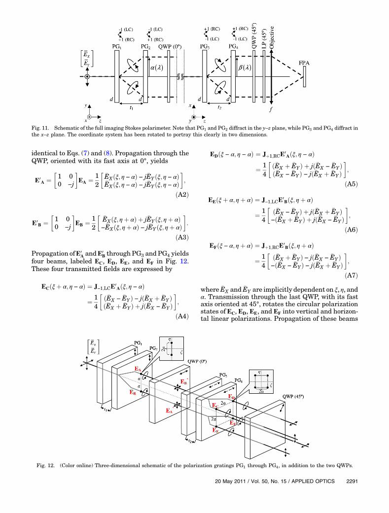
identical to Eqs. (7) and (8). Propagation through theQWP, oriented with its fast axis at 0°, yields

E0A ¼

�1 00 −j

�EA ¼ 1

2

��EXðξ; η − αÞ − j�EYðξ; η − αÞ�EXðξ; η − αÞ − j�EYðξ; η − αÞ

�;

ðA2Þ

E0B ¼

�1 00 −j

�EB ¼ 1

2

��EXðξ; ηþ αÞ þ j�EYðξ; ηþ αÞ−�EXðξ; ηþ αÞ − j�EYðξ; ηþ αÞ

�:

ðA3Þ

Propagation ofE0A andE0

B throughPG3 andPG4 yieldsfour beams, labeled EC, ED, EE, and EF in Fig. 12.These four transmitted fields are expressed by

ECðξþ α; η − αÞ ¼ J−1;LCE0Aðξ; η − αÞ

¼ 14

�ð�EX − �EYÞ − jð�EX þ �EYÞð�EX þ �EYÞ þ jð�EX − �EYÞ

�;

ðA4Þ

EDðξ − α; η − αÞ ¼ Jþ1;RCE0Aðξ; η − αÞ

¼ 14

�ð�EX þ �EYÞ þ jð�EX − �EYÞð�EX − �EYÞ − jð�EX þ �EYÞ

�;

ðA5Þ

EEðξþ α; ηþ αÞ ¼ J−1;LCE0Bðξ; ηþ αÞ

¼ 14

�ð�EX − �EYÞ þ jð�EX þ �EYÞ−ð�EX þ �EYÞ þ jð�EX − �EYÞ

�;

ðA6Þ

EFðξ − α; ηþ αÞ ¼ Jþ1;RCE0Bðξ; ηþ αÞ

¼ 14

�ð�EX þ �EYÞ − jð�EX − �EYÞ−ð�EX − �EYÞ − jð�EX þ �EYÞ

�;

ðA7Þ

where �EX and �EY are implicitly dependent on ξ, η, andα. Transmission through the last QWP, with its fastaxis oriented at 45°, rotates the circular polarizationstates of EC, ED, EE, and EF into vertical and horizon-tal linear polarizations. Propagation of these beams

Fig. 11. Schematic of the full imaging Stokes polarimeter. Note that PG1 and PG2 diffract in the y–z plane, while PG3 and PG4 diffract inthe x–z plane. The coordinate system has been rotated to portray this clearly in two dimensions.

Fig. 12. (Color online) Three-dimensional schematic of the polarization gratings PG1 through PG4, in addition to the two QWPs.


through the analyzing linear polarizer unifies theminto a 45° linear polarization state. The complete elec-tric field’s x and y components incident on the lens is

ELX ¼ EL

Y

¼ 14ð�EXðξþ α; η − αÞ − j�EYðξþ α; η − αÞÞ

þ ð�EXðξ − α; η − αÞ − j�EYðξ − α; η − αÞÞþ ðj�EXðξþ α; ηþ αÞ − �EYðξþ α; ηþ αÞÞþ ð−j�EXðξ − α; ηþ αÞ þ �EYðξ − α; ηþ αÞÞ: ðA8Þ

The objective lens produces a Fourier transformationof the field. Performing this on the EL

X componentyields

EL ¼ F½ELX�ξ¼ x

λf ;η¼ yλf

¼ 14ð�EX − j�EYÞej

2πλf αðx−yÞ þ ð−j�EX þ �EYÞe−j

2πλf αðx−yÞ

þ ðj�EX − �EYÞej2πλf αðxþyÞ þ ð�EX − j�EYÞe−j

2πλf αðxþyÞ;

ðA9Þ

where �EX and �EY are implicitly dependent on x and y,f is the focal length of the objective lens, and λ is thewavelength of the incident illumination. The inten-sity is calculatedby taking the absolute value squaredof EL. Simplifying the expression with the Stokesparameter definitions, combining terms into cosinesand sines, and substituting the shear α from Eq. (9),produces the final intensity pattern on the FPA:

Iðx; yÞ ¼ 12S0ðx; yÞ þ

12S3ðx; yÞ cos

�2π 2mt

fΛ x

�

þ 14S2ðx; yÞ

�cos

�2π 2mt

fΛ ðx − yÞ�

− cos�2π 2mt

fΛ ðxþ yÞ��

þ 14S1ðx; yÞ

�sin

�2π 2mt

fΛ ðx − yÞ�

þ sin�2π 2mt

fΛ ðxþ yÞ��

: ðA10Þ

This configuration enables the measurement of allfour Stokes parameters by isolating the variouswhite-light spatial carrier frequencies U1 and U2,defined as

U1 ¼ 2mtfΛ ; ðA11Þ

U2 ¼ 2ffiffiffi2

p mtfΛ : ðA12Þ

For the purposes of this paper, only the linear polari-meter implementation was experimentally verifieddue to the availability of the polarization gratings.

M. J. Escuti acknowledges support from theNational Science Foundation (NSF, grant ECCS-0955127).

References1. J. S. Tyo, D. L. Goldstein, D. B. Chenault, and J. A. Shaw,

“Review of passive imaging polarimetry for remote sensing ap-plications,” Appl. Opt. 45, 5453–5469 (2006).

2. E. R. Cochran and C. Ai, “Interferometric stress birefringencemeasurement,” Appl. Opt. 31, 6702–6706 (1992).

3. K. Oka and T. Kaneko, “Compact complete imaging polari-meter using birefringent wedge prisms,” Opt. Express 11,1510–1519 (2003).

4. K. Oka and N. Saito, “Snapshot complete imaging polarimeterusing Savart plates,” Proc. SPIE 6295, 629508 (2006).

5. J. VanDelden, “Interferometric polarization interrogatingfilter assembly and method,” U.S. patent 6,674,532 B2(6 January 2004).

6. M. W. Kudenov, M. E. L. Jungwirth, E. L. Dereniak, and G. R.Gerhart, “White light Sagnac interferometer for snapshotlinear polarimetric imaging,” Opt. Express 17, 22520–22534(2009).

7. M. Mujat, E. Baleine, and A. Dogariu, “Interferometric ima-ging polarimeter,” J. Opt. Soc. Am. A 21, 2244–2249 (2004).

8. M. W. Kudenov, L. Pezzaniti, E. L. Dereniak, and G. R.Gerhart, “Prismatic imaging polarimeter calibration for theinfrared spectral region,” Opt. Express 16, 13720–13737(2008).

9. K. Oka, R. Suda, M. Ohnuki, D. Miller, and E. L. Dereniak,“Snapshot imaging polarimeter for polychromatic light usingSavart plates and diffractive lenses,” in Frontiers in Optics,OSA Technical Digest (CD) (Optical Society of America,2009), paper FThF4.

10. C. Oh, J. Kim, J. F. Muth, S. Serati, and M. J. Escuti,“High-throughput, continuous beam steering using rotatingpolarization gratings,” IEEE Photon. Technol. Lett. 22,200–202 (2010).

11. J. C. Wyant, “OTFmeasurements with a white light source: aninterferometric technique,” Appl. Opt. 14, 1613–1615 (1975).

12. L. Nikolova and T. Todorov, “Diffraction efficiency and selec-tivity of polarization holographic recording,” Opt. Acta 31,579–588 (1984).

13. J. Tervo and J. Turunen, “Paraxial-domain diffractive ele-ments with 100% efficiency based on polarization gratings,”Opt. Lett. 25, 785–786 (2000).

14. C. Oh and M. J. Escuti, “Numerical analysis of polarizationgratings using the finite-difference time-domain method,”Phys. Rev. A 76, 043815 (2007).

15. C. Oh and M. J. Escuti, “Achromatic diffraction from polariza-tion gratings with high efficiency,” Opt. Lett. 33, 2287–2289(2008).

16. G. P. Crawford, J. N. Eakin, M. D. Radcliffe, A. C. Jones, andR. A. Pelcovits, “Liquid-crystal diffraction gratings using po-larization holography alignment techniques,” J. Appl. Phys.98, 123102 (2005).

17. M. J. Escuti, C. Oh, C. Sanchez, C. W. M. Bastiaansen, andD. J. Broer, “Simplified spectropolarimetry using reactivemesogen polarization gratings,” Proc. SPIE 6302, 630207(2006).

18. R. K. Komanduri, W. M. Jones, C. Oh, and M. J. Escuti, “Po-larization-independent modulation for projection displays


using small-period LC polarization gratings,” J. Soc. Inf. Disp.15, 589–594 (2007).

19. S. Pancharatnam, “Generalized theory of interference, and itsapplications. Part I. Coherent pencils,” Proc. Indian Acad. Sci.A 44, 247–262 (1956).

20. M. V. Berry, “The adiabatic phase and Pancharatnam’s phasefor polarized light,” J. Mod. Opt. 34, 1401–1407 (1987).

21. D. Goldstein, Polarized Light (Marcel Dekker, 2003).22. J. Craven and M. W. Kudenov, “False signature reduction in

channeled spectropolarimetry,” Opt. Eng. 49, 053602 (2010).23. J. S. Tyo, E. N. Pugh, and N. Engheta, “Colorimetric represen-

tations for use with polarization-difference imaging of ob-jects in scattering media,” J. Opt. Soc. Am. A 15, 367–374(1998).


Documents

White-light channeled imaging polarimeter using broadband ... · White-light channeled imaging polarimeter using broadband polarization gratings Michael W. Kudenov,1,* Michael J