50 English Edition No.42 July 2014

Feature ArticleApplication

Wheel Slip Simulation for Dynamic Road Load SimulationFeature Article Application� Reprint�of�Readout�No.�38

Wheel Slip Simulation for Dynamic Road Load Simulation

Bryce JohnsonIncreasingly stringent fuel economy standards are forcing automobile

manufacturers to search for efficiency gains in every part of the drive train

from engine to road surface. Safety mechanisms such as stability control and

anti-lock braking are becoming more sophisticated. At the same time drivers

are demanding higher performance from their vehicles. Hybrid transmissions

and batteries are appearing in more vehicles. These issues are forcing the

automobile manufacturers to require more from their test stands. The test stand

must now simulate not just simple vehicle loads such as inertia and windage,

but the test stand must also simulate driveline dynamic loads. In the past,

dynamic loads could be simulated quite well using Service Load Replication

(SLR*1). However, non-deterministic events such as the transmission shifting or

application of torque vectoring from an on board computer made SLR unusable

for the test. The only way to properly simulate driveline dynamic loads for non-

deterministic events is to provide a wheel-tire-road model simulation in addition

to vehicle simulation. The HORIBA wheel slip simulation implemented in the

SPARC power train controller provides this wheel-tire-road model simulation.

*1: Service load replication is a frequency domain transfer function calculation with iterative convergence to a solution. SLR uses field collected, time history format data.

Introduction

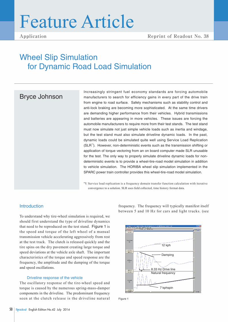
To understand why tire-wheel simulation is required, we should first understand the type of driveline dynamics that need to be reproduced on the test stand. Figure 1 is the speed and torque of the lef t wheel of a manual transmission vehicle accelerating aggressively from rest at the test track. The clutch is released quickly and the tire spins on the dry pavement creating large torque and speed deviations at the vehicle axle shaft. The important characteristics of the torque and speed response are the frequency, the amplitude and the damping of the torque and speed oscillations.

Driveline response of the vehicleThe oscillatory response of the tire-wheel speed and torque is caused by the numerous spring-mass-damper components in the driveline. The predominant frequency seen at the clutch release is the d r ivel ine natural

frequency. The frequency will typically manifest itself between 5 and 10 Hz for cars and light trucks. (see

7 kphspin

12 kph

8.33 Hz Drive lineNatural frequency

Damping

Figure 1

51English Edition No.42 July 2014

Technical ReportsFeature Article Application� Reprint�of�Readout�No.�38

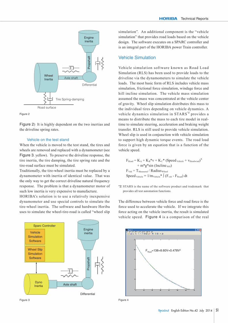
Figure 2) It is highly dependent on the two inertias and the driveline spring rates.

Vehicle on the test standWhen the vehicle is moved to the test stand, the tires and wheels are removed and replaced with a dynamometer (see Figure 3. yellow). To preserve the driveline response, the tire inertia, the tire damping, the tire spring rate and the tire-road surface must be simulated. Traditionally, the tire-wheel inertia must be replaced by a dynamometer with inertia of identical value. That was the only way to get the correct driveline natural frequency response. The problem is that a dynamometer motor of such low inertia is very expensive to manufacture.HORIBA’s solution is to use a relatively inexpensive dynamometer and use special controls to simulate the tire-wheel inertia. The software and hardware Horiba uses to simulate the wheel-tire-road is called “wheel slip

simulation”. An additional component is the “vehicle simulation” that provides road loads based on the vehicle design. The software executes on a SPARC controller and is an integral part of the HORIBA power Train controller.

Vehicle Simulation

Vehicle simulat ion sof tware known as Road Load Simulation (RLS) has been used to provide loads to the driveline via the dynamometers to simulate the vehicle loads. The most basic form of RLS includes vehicle mass simulation, frictional force simulation, windage force and hill incline simulation. The vehicle mass simulation assumed the mass was concentrated at the vehicle center of gravity. Wheel slip simulation distributes this mass to the individual tires depending on vehicle dynamics. A vehicle dynamics simulation in STARS*2 provides a means to distribute the mass to each tire model in real-time to simulate steering, acceleration and braking weight transfer. RLS is still used to provide vehicle simulation. Wheel slip is used in conjunction with vehicle simulation to support high dynamic torque events. The road load force is given by an equation that is a function of the vehicle speed.

FRoad = KA + KB*v + KC* (Speed Vehicle + vHeadwind)X + m*g*sin (Incline Hill)

FVeh = TMeasured / RadiusWheel

Speed Vehicle = 1/mVehicle* ∫ (Fveh - FRoad) dt

*2: STARS is the name of the software product and trademark that provides all test automation functions.

The difference between vehicle force and road force is the force used to accelerate the vehicle. If we integrate this force acting on the vehicle inertia, the result is simulated vehicle speed. Figure 4 is a comparison of the real

WheelInertia

Tire Spring-damping

Road surface

Axle shaft

DifferentialProps

haft

Engineinertia

Figure 2

Axle shaft

Differential

Pro

psha

ft

Engineinertia

DynoInertia

Sparc Controller

Wheel SlipSimulationSoftware

VehicleSimulationSoftware

Figure 3

FRoad=138+8.60V+0.478V2

Figure 4

52 English Edition No.42 July 2014

Feature ArticleApplication

Wheel Slip Simulation for Dynamic Road Load Simulation

vehicle and a simulated vehicle during a coast from 50 mph to zero. This comparison shows how well the simulation (green) matches the real vehicle (blue).

Wheel slip simulationThere are 3 characteristics of the test stand that must be controlled to get proper dr ivelive dynamics in the simulation. First, the tire forces and tire slip must be simulated using a tire model. Second, the wheel-tire inertia must be simulated to get the proper drive line natural frequency. Third, the damping of the oscillations must be controlled.

The tire model, what is slip?Most of us are intimately familiar with tire spin events when a tire spins on wet roads or ice. However, not everyone understands that the tire is always slipping sl ightly; even when a vehicle is moving on a d r y pavement. Figure 5 is the data from a real vehicle at a test track on dry pavement. The vehicle speed is 39.4 kph, the front tire speed is 367 rpm and the rear wheel speed is 383 rpm. This is a rear wheel drive vehicle whose rear tires are transferring 4600 N of force. What is seen in this graph is that the rear tires are rotating 16 rpm faster than the front tires. Saying another way, the rear tires are slipping at 16 rpm on the road surface when rotating at 383 rpm while transferring 4600 N of force.

What we find is that vehicle tires slip at a rate proportional to the amount of force they transfer to the road surface. This slippage is what is referred to as wheel slip. If we continue to increase the tire force by accelerating the vehicle more aggressively, a maximum force will be reached and the tire will slip quite dramatically as the tire on ice. One often says the tire is spinning. The test stand

must implement a tire model to reproduce this force-slip functionality. The definition of slip is: Slip= (VTire-VVehicle) / VVehicle. If we take vehicle speed as the front tire speed or 367 rpm and the tire speed as the rear tire speed or 383 rpm, we get a slip of 4.4%.

Simulation of tire forces and slip using PacejkaThe traditional way to simulate tire forces and slip is to use a tire model. The traditional tire model describes a functional relationship between slip of the tire and the force transferred through the tire. Although there are a number of tire models in the literature, one of the most well known tire models is the Pacejka-96 longitudinal tire model. This is function that describes the tire force as a function of tire slip. The Pacejka function is F = D sin (b0 tan-1 (SB + E (tan-1 (SB) - SB))). “F” is tire force and “S” is tire slip. The parameters D, B, E and S are values based on the tire normal force and the Pacejka parameters b0 to b10. The value Fz is the normal force applied to the wheel. By adjusting the normal force of each tire in real-time using STARS, the test engineer accounts for vehicle body movements that change the weight distribution of the vehicle. (Figure 6)

mup = b1 Fz + b2

D = mup Fz

B = (b3 Fz + b4) e -b5 Fz / (b0 mup)E = b6 Fz

2 + b7 Fz + b8

S = 100 Sfrac + b9 Fz + b10

Simulation of tire forces and slip using a simple model

Quite often, the test engineer does not have access to the Pacejka parameters. In such a case, the customer can use a simple model to describe the tire forces and slip. The

Vehicle speed = 39.6 kph

Non-drive front tire = 367 rpm

Torque producing rear tire 383 rpm

Figure 5

NormalForce N

TireForce Nb0 = 1.65b1 = 0b2 = 1688b3 = 0b4 = 229b5 = 0b6 = 0b7 = 0b8 =-10b9 = 0b10 = 0

Slip %

0 %20 %

-20 %

Figure 6

53English Edition No.42 July 2014

Technical Reports

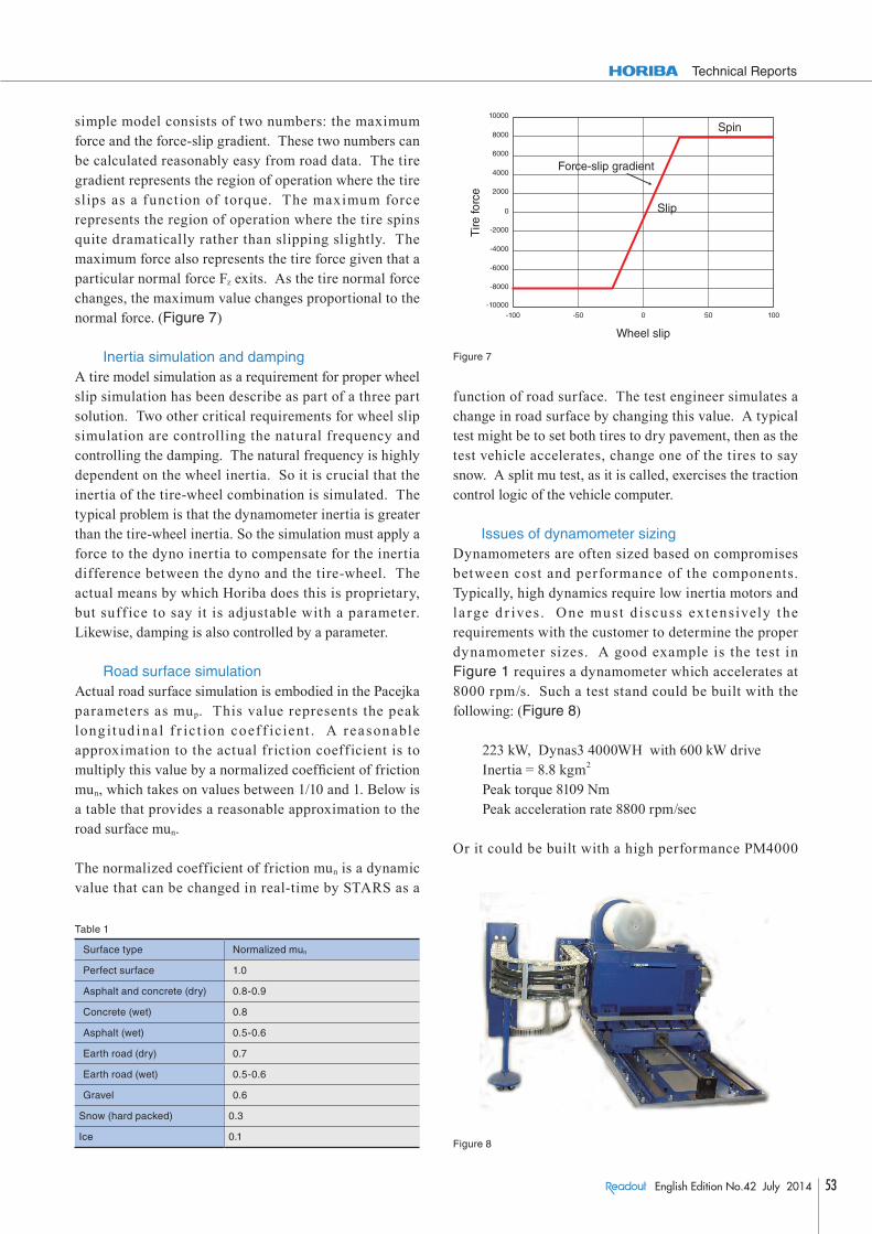
simple model consists of two numbers: the maximum force and the force-slip gradient. These two numbers can be calculated reasonably easy from road data. The tire gradient represents the region of operation where the tire slips as a function of torque. The maximum force represents the region of operation where the tire spins quite dramatically rather than slipping slightly. The maximum force also represents the tire force given that a particular normal force Fz exits. As the tire normal force changes, the maximum value changes proportional to the normal force. (Figure 7)

Inertia simulation and dampingA tire model simulation as a requirement for proper wheel slip simulation has been describe as part of a three part solution. Two other critical requirements for wheel slip simulation are controlling the natural frequency and controlling the damping. The natural frequency is highly dependent on the wheel inertia. So it is crucial that the inertia of the tire-wheel combination is simulated. The typical problem is that the dynamometer inertia is greater than the tire-wheel inertia. So the simulation must apply a force to the dyno inertia to compensate for the inertia difference between the dyno and the tire-wheel. The actual means by which Horiba does this is proprietary, but suff ice to say it is adjustable with a parameter. Likewise, damping is also controlled by a parameter.

Road surface simulationActual road surface simulation is embodied in the Pacejka parameters as mup. This value represents the peak long it ud inal f r ic t ion coef f ic ient . A reasonable approximation to the actual friction coefficient is to multiply this value by a normalized coefficient of friction mun, which takes on values between 1/10 and 1. Below is a table that provides a reasonable approximation to the road surface mun.

The normalized coefficient of friction mun is a dynamic value that can be changed in real-time by STARS as a

function of road surface. The test engineer simulates a change in road surface by changing this value. A typical test might be to set both tires to dry pavement, then as the test vehicle accelerates, change one of the tires to say snow. A split mu test, as it is called, exercises the traction control logic of the vehicle computer.

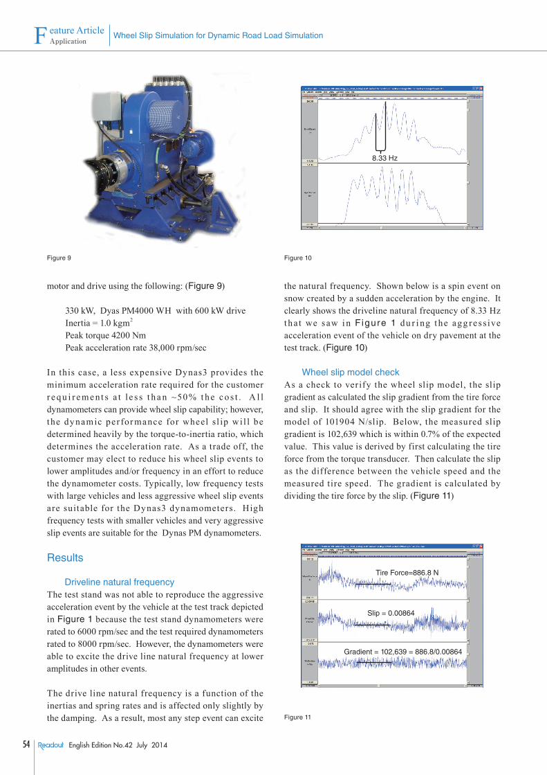
Issues of dynamometer sizingDynamometers are often sized based on compromises between cost and performance of the components. Typically, high dynamics require low inertia motors and la rge d r ives . One must d iscuss extensively the requirements with the customer to determine the proper dynamometer sizes. A good example is the test in Figure 1 requires a dynamometer which accelerates at 8000 rpm/s. Such a test stand could be built with the following: (Figure 8)

223 kW, Dynas3 4000WH with 600 kW driveInertia = 8.8 kgm2

Peak torque 8109 NmPeak acceleration rate 8800 rpm/sec

Or it could be built with a high performance PM4000

Figure 8

Wheel slip

Tire

forc

e

Force-slip gradient

Slip

Spin

-10000

-8000

-6000

8000

10000

-4000

-2000

0

2000

4000

6000

-100 -50 0 50 100

Figure 7

Table 1

Surface type Normalized mun

Perfect surface 1.0

Asphalt and concrete (dry) 0.8-0.9

Concrete (wet) 0.8

Asphalt (wet) 0.5-0.6

Earth road (dry) 0.7

Earth road (wet) 0.5-0.6

Gravel 0.6

Snow (hard packed) 0.3

Ice 0.1

54 English Edition No.42 July 2014

Feature ArticleApplication

Wheel Slip Simulation for Dynamic Road Load Simulation

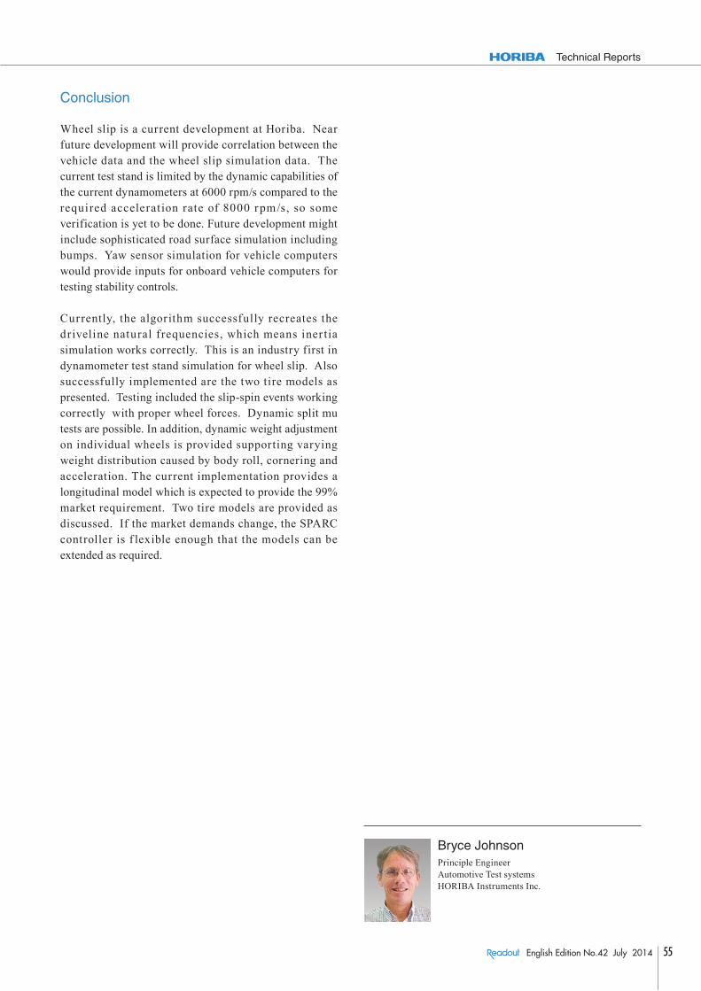
motor and drive using the following: (Figure 9)

330 kW, Dyas PM4000 WH with 600 kW driveInertia = 1.0 kgm2

Peak torque 4200 NmPeak acceleration rate 38,000 rpm/sec

In this case, a less expensive Dynas3 provides the minimum acceleration rate required for the customer r e q u i r e me n t s a t l e s s t h a n ~50 % t he c o s t . A l l dynamometers can provide wheel slip capability; however, the dy namic per for mance for wheel sl ip wi l l be determined heavily by the torque-to-inertia ratio, which determines the acceleration rate. As a trade off, the customer may elect to reduce his wheel slip events to lower amplitudes and/or frequency in an effort to reduce the dynamometer costs. Typically, low frequency tests with large vehicles and less aggressive wheel slip events are suitable for the Dynas3 dynamometers. High frequency tests with smaller vehicles and very aggressive slip events are suitable for the Dynas PM dynamometers.

Results

Driveline natural frequencyThe test stand was not able to reproduce the aggressive acceleration event by the vehicle at the test track depicted in Figure 1 because the test stand dynamometers were rated to 6000 rpm/sec and the test required dynamometers rated to 8000 rpm/sec. However, the dynamometers were able to excite the drive line natural frequency at lower amplitudes in other events.

The drive line natural frequency is a function of the inertias and spring rates and is affected only slightly by the damping. As a result, most any step event can excite

the natural frequency. Shown below is a spin event on snow created by a sudden acceleration by the engine. It clearly shows the driveline natural frequency of 8.33 Hz t ha t we saw i n Figure 1 du r i ng t he agg re ss ive acceleration event of the vehicle on dry pavement at the test track. (Figure 10)

Wheel slip model checkAs a check to verify the wheel slip model, the slip gradient as calculated the slip gradient from the tire force and slip. It should agree with the slip gradient for the model of 101904 N/slip. Below, the measured slip gradient is 102,639 which is within 0.7% of the expected value. This value is derived by first calculating the tire force from the torque transducer. Then calculate the slip as the difference between the vehicle speed and the measured tire speed. The gradient is calculated by dividing the tire force by the slip. (Figure 11)

Figure 9

8.33 Hz

Figure 10

Tire Force=886.8 N

Slip = 0.00864

Gradient = 102,639 = 886.8/0.00864

Figure 11

55English Edition No.42 July 2014

Technical Reports

Conclusion

Wheel slip is a current development at Horiba. Near future development will provide correlation between the vehicle data and the wheel slip simulation data. The current test stand is limited by the dynamic capabilities of the current dynamometers at 6000 rpm/s compared to the required accelerat ion rate of 8000 rpm/s, so some verification is yet to be done. Future development might include sophisticated road surface simulation including bumps. Yaw sensor simulation for vehicle computers would provide inputs for onboard vehicle computers for testing stability controls.

Currently, the algorithm successfully recreates the driveline natural frequencies, which means iner tia simulation works correctly. This is an industry first in dynamometer test stand simulation for wheel slip. Also successfully implemented are the two tire models as presented. Testing included the slip-spin events working correctly with proper wheel forces. Dynamic split mu tests are possible. In addition, dynamic weight adjustment on individual wheels is provided supporting varying weight distribution caused by body roll, cornering and acceleration. The current implementation provides a longitudinal model which is expected to provide the 99% market requirement. Two tire models are provided as discussed. If the market demands change, the SPARC controller is f lexible enough that the models can be extended as required.

Bryce JohnsonPrinciple EngineerAutomotive Test systemsHORIBA Instruments Inc.