What would Nelson and Plosser �nd had they used panelunit root tests?�

Christophe Hurlin y

Revised Version. June 2007

Abstract

In this study, we systemically apply nine recent panel unit root tests to the samefourteen macroeconomic and �nancial series as those considered in the seminalpaper by Nelson and Plosser (1982). The data cover OECD countries from 1950to 2003. Our results clearly point out the di¢ culty that applied econometricianswould face when they want to get a simple and clear-cut diagnosis with panelunit root tests. We con�rm the fact that panel methods must be very carefullyused for testing unit roots in macroeconomic or �nancial panels. More precisely,we �nd mitigated results under the cross-sectional independence assumption, sincethe unit root hypothesis is rejected for many macroeconomic variables. Wheninternational cross-correlations are taken into account, conclusions depend on thespeci�cation of these cross-sectional dependencies. Two groups of tests can bedistinguished. The �rst group tests are based on a dynamic factor structure oran error component model. In this case, the non stationarity of common factors(international business cycles or growth trends) is not rejected, but the results areless clear with respect to idiosyncratic components. The second group tests arebased on more general speci�cations. Their results are globally more favourable tothe unit root assumption.

� Key Words : Unit Root Tests, Panel Data.� J.E.L Classi�cation : C23, C33

�I am grateful to Benoit Perron, Rafal Kierzenkowski and Regis Breton for helpful commentsand suggestions. I am grateful to Faouzi Boujedra for research assistance. All the tests used havebeen programmed under Matlab. Codes and data are available on the website: http://www.univ-orleans.fr/deg/masters/ESA/CH/churlin_R.htm

yLEO, University of Orléans. Rue de Blois. BP 6739. 45067 Orléans Cedex 2. France. E-mailaddress: christophe.hurlin@univ-orleans.fr.

1

1 Introduction

Many studies have been devoted to the �nite sample properties of panel unit root

tests. In this literature, it is now standard to distinguish �rst generation tests that

are based on the assumption of independent cross section units and second generation

tests that allow for cross-section dependence (see Banerjee, 1999; Baltagi and Kao, 2000;

Choi, 2004; Hurlin and Mignon, 2004; Breitung and Pesaran, 2005 for a survey). The

empirical power and size of �rst generation unit root tests have been simulated under

various assumptions in Maddala and Wu (1999), Levin, Lin and Chu (2002), Choi

(1999, 2001), Breitung (2000), Banerjee, Marcellino and Osbat (2005). The relative

performance of second generation unit root tests has been studied in particular by

Gutierrez (2003, 2005), Gengenbach, Palm, and Urbain (2004) or Baltagi, Bresson and

Pirotte (2005). The results of these studies depend very much on the underlying data

generating process used in the Monte Carlo simulations. In particular, it appears that

the �nite sample properties of panel unit root tests depend on (i) the homogeneity

assumption used under the alternative, (ii) the existence of cross-section dependences,

(iii) the speci�cation of these cross-section dependences (factor structure or weak cross

section dependence), (iv) the relative sample sizes T and N , (v) the existence of long-

run cross-unit relationships, etc.. In many con�gurations, the panel unit root tests

have severe size biases in �nite samples. In some cases, the empirical size of the tests is

substantially higher than the nominal level, so that the null hypothesis of a unit root

is rejected very often, even if correct. It is for instance the case when the assumption

of no cross-unit correlation or cross-unit cointegrating is violated and �rst generation

unit root tests are used (Banerjee, Marcellino and Osbat, 2005). But, it may be also

the case when second generation unit root tests are used in a context of cross-unit

dependences for which they are not designed. The use of a factor model (Bai and Ng,

2004) in the case of weak correlation may do not yield valid test procedures. On the

contrary, the use of unit root tests that allow for weak dependence may also lead to

severe size biases in some cases1. Given these results, some authors warn against the

1 It is for instance the case, when the cross-section dependences are speci�ed as standard spatialerror processes (Baltagi, Bresson and Pirotte, 2005) and nonlinear IV tests (Chang, 2002) or bootstrapbased tests (Chang, 2004) are used.

2

use of panel methods for testing for unit roots in some cases. In particular, Banerjee,

Marcellino and Osbat (2005) clearly ask the question: should we use panel methods for

testing for PPP?

In this perspective, our paper aims to evaluate the advantages and drawbacks of

panel unit root tests for macroeconomic and �nancial series. But, our methodological

approach is di¤erent from the approaches previously mentioned. Rather than simulat-

ing some Monte Carlo experiments and evaluating empirical size and power in many

di¤erent con�gurations, we propose here to respond to the question: what results would

Nelson and Plosser (1982) obtain if they have used panel unit root tests2? For that, we

systemically apply panel unit root tests to the same 14 macroeconomic and �nancial

variables (including measures of output spending, money, prices and interest rates) as

those studied by Nelson and Plosser. The series are considered for a panel of OECD

countries over the period 1950-2003 given data availability. More precisely, we consider

nine panel unit root tests among the most used in the literature. Four �rst generation

tests are studied: (i) the tests of Levin, Lin and Chu (2002) based on a homogenous

alternative assumption, (ii) the tests of Im, Pesaran and Shin (2003) that allow for a

heterogeneous alternative and the Fisher type tests of (iii) Maddala and Wu (1999) and

(iv) Choi (2001). The common feature of these �rst generation tests is the restriction

that all cross-sections are independent. However, it is well-known that this cross-unit

independence assumption is quite restrictive in many empirical applications. So, we

also consider some second generation unit root tests that allow cross-unit dependencies.

A growing literature is now devoted to these tests with among others, the papers by Bai

and Ng (2004), Choi (2002), Phillips and Sul (2003), Moon and Perron (2004), Pesaran

(2004) and Chang (2002, 2004). The main issue is to specify the cross-sectional depen-

dencies, since as pointed out by Quah (1994), individual observations in a cross-section

have no natural ordering. Consequently, various speci�cations and a lot of di¤erent

testing procedures have been proposed. In our study, we consider two groups of tests.

The �rst group tests are based on a dynamic factor model (Bai and Ng, 2004; Moon

2Based on standard time series unit root tests, the seminal paper by Nelson and Plosser pointed outthat American macroeconomic series feature, quasi systematically, stochastic tendencies and unit rootproperties.

3

and Perron, 2004; Pesaran, 2003) or an error-component model (Choi, 2002). The

cross-sectional dependency is then due to the presence of one or more common factors

or to a random time e¤ect. The tests of the second group are de�ned by opposition

to these speci�cations based on common factor or time e¤ects. In this group, some

speci�c (O�Connell, 1998; Taylor and Sarno, 1998) or more general (Chang, 2002 and

2004) speci�cations of the cross-sectional correlations are proposed in the literature.

Here, we limit our analysis to the IV nonlinear test proposed by Chang (2002).

Contrary to a standard �nite sample exercise based on Monte Carlo simulations,

our approach does not allow determining what the most robust test is (since we do

not know the true data generating process). We can not give some recommendations

about the appropriate circumstances for using each test. However, our study clearly

points out the di¢ culty that applied econometricians would face when they want to get

a simple and clear-cut diagnosis with panel unit root tests. They con�rm the fact that

one must be very careful with the use of panel root tests on macroeconomic time series.

In particular, we highlight the in�uence of (i) the heterogeneous speci�cation of the

model, (ii) the cross-sectional independence assumption and the (iii) the speci�cation

of these dependences.

The rest of the paper is organized as follows. In section 2, we present the data and

the results of three �rst generation tests. Section 3 presents the results obtained from

�ve representative tests of the second generation. The last section concludes.

2 First Generation Unit Root Tests

What would Nelson and Plosser �nd had they used �rst generation panel unit root

tests? To answer this question, we consider in this study the same series as those

used in the seminal paper of Nelson and Plosser (1982). The only di¤erence is that

we consider these series for a panel of OECD countries3. The data are annual with

starting dates from 1952 to 1971 and ending dates from 2000 to 2003. This sample size

3The second slight di¤erence is that we consider GDP (and GDP per capita, real GDP) rather thanGNP for data availability.

4

is relatively short compared to the sample used initially for the United States by Nelson

and Plosser (from 1860 or 1909 to 1970 according to the series), but it corresponds to

that of most of macroeconomic or �nancial panels. Since some panel unit root tests

require the use of a balanced panel, for each variable we consider the same balanced

database for all the tests. The data includes the maximum of OECD countries given

the data availability. The lists of countries and data sources are reported in appendix

A.

2.1 Levin and Lin unit root tests

One of the most popular �rst generation unit root test is undoubtedly the test proposed

by Levin, Lin and Chu (2002). Let us consider a variable observed on N countries and

T periods and a model with individual e¤ects and no time trends. As it is well known,

Levin and Lin (LL thereafter) consider a model in which the coe¢ cient of the lagged

dependent variable is restricted to be homogenous across all units of the panel:

�yit = �i + � yi;t�1 +

piXz=1

�i;z�yi;t�z + "it (1)

for i = 1; ::; N and t = 1; ::; T . The errors "it i:i:d:�0; �2"i

�are assumed to be inde-

pendent across the units of the sample. In this model, LL are interested in testing

the null hypothesis H0 : � = 0 against the alternative hypothesis H1 : � = �i < 0

for all i = 1; ::N , with auxiliary assumptions about the individual e¤ects (�i = 0

for all i = 1; ::N under H0). This restrictive alternative hypothesis implies that the

autoregressive parameters are identical across the panel.

In a model with individual e¤ects, the standard t-statistic t� based on the pooled

estimator b� diverges to negative in�nity. That is why, LL suggest using the followingadjusted t-statistic:

t�� =t���T

�N T bSN � b�b�b�2e"��

��T��T

�(2)

where the mean adjustment ��T and standard deviation adjustment ��T are simulated by

authors (Levin, Lin and Chu, 2002, table 2) for various sample sizes T . The adjustment

term is also function of the average of individual ratios of long-run to short-run vari-

ances, bSN = (1=N)PNi=1 b�yi/b�"i ; where b�yi denotes a kernel estimator of the long-run

5

variance for the country i. LL suggest using a Bartlett kernel function and a homo-

geneous truncation lag parameter given by the simple formula K = 3:21T 1=3. They

demonstrate that, under the non stationary null hypothesis, the adjusted t-statistic t��

converges to a standard normal distribution.

The results of the LL tests in a model with individual e¤ects are reported in table 1.

In order to assess the sensitivity of the results to the choice of the kernel function and

the selection of the bandwidth parameters in the adjustment terms, for each variable

we compute three statistics. The �rst one, denoted t��, is based on a Bartlett kernel

function and the common lag truncation parameter K proposed by LL. The second

statistic, denoted t�B� , is also based on a Bartlett kernel but with individual lag trunca-

tion parameters selected according the Newey and West�s procedure (1994). The last

statistic, denoted t�C� , is computed with a Quadratic Spectral kernel and individual lag

truncation parameters. Finally, we also consider a model with individual e¤ects and

deterministic trends to asses the sensitivity of our results to the speci�cation of the

deterministic component. The corresponding adjusted t-statistic based on a Bartlett

kernel is denoted t�C3 :

The results would have surprised Nelson and Plosser. The LL tests clearly indicate

that stationarity is a common feature of the main macroeconomic variables. Indeed,

at a 5% signi�cance level, the tests strongly reject the null of non stationarity for 11

macroeconomic series out of 14, including real GDP, nominal GDP, employment etc.

The unit root hypothesis is not rejected only for bond yield, common stock prices and

velocity. Besides, except for velocity, these results are robust to the choice of kernel

function and bandwidth parameter. These conclusions, except for the unemployment

rate and the money stock, are also robust to the speci�cation of the deterministic

component, i:e: with or without time trends. Various explanations to these surprising

results are possible. The �rst one is based on the mispeci�cation of one or more on

the N individual ADF lag lengths in the model (1). Im, Pesaran and Shin (2003)

show the importance of correctly choosing these individual lag orders for the LL tests.

In our study, individual lag lengths are optimally chosen using the general-to-speci�c

6

(GS) procedure of Hall (1994) with a maximum lag length set to 4. However, similar

qualitative results (not reported) are obtained when individual lag lengths are chosen

by information criteria (AIC or BIC).

Then, others explanations must be evoked. The second one is linked to the restric-

tive homogeneous assumption used in LL. In particular, this assumption implies that

all panel members are forced to have identical orders of integration. The null hypoth-

esis is that all series contain a unit root, while the alternative hypothesis is that no

series contains a unit root, that is, all are stationary. Then with as few as one station-

ary series, the rejection rate rises above the nominal size of the test, and continues to

increase with the number of I(0) series in the panel.

2.2 Heterogeneous Panel Unit Root Tests

At this stage, the question is: if Nelson and Plosser would have used heterogeneous panel

unit root tests, would they have also concluded to non stationarity of macroeconomic

and �nancial variables? In order to answer this question, we consider two heteroge-

neous tests based on the cross-sectional independence assumption: the well-known test

proposed by Im, Pesaran and Shin (2003) (IPS thereafter) and two equivalent Fisher

type tests (Choi, 1999; Maddala and Wu, 1999). It is well known that the main advan-

tage of these test compared to LL one, is to allow for heterogeneity in the value of �i

under the alternative hypothesis. The corresponding model with individual e¤ects and

no time trend becomes:

�yit = �i + �iyi;t�1 +

piXz=1

�i;z�yi;t�z + "it (3)

The null hypothesis is de�ned as H0 : �i = 0 for all i = 1; ::N and the alternative

hypothesis isH1 : �i < 0 for i = 1; ::N1 and �i = 0 for i = N1+1; ::; N; with 0 < N1 � N .

The alternative hypothesis allows unit roots for some (but not all) of the individual. In

this context, the IPS test is based on the (augmented) Dickey-Fuller statistics averaged

across groups. Let tiT (pi; �i) with �i =��i;1; ::; �i;pi

�denote the t-statistic for testing

7

unit root in the ith country. The IPS statistic is then de�ned as:

t_barNT =1

N

NXi=1

tiT (pi; �i) (4)

Under the assumption of cross-sectional independence, this statistic is shown to

sequentially converge to a normal distribution. IPS propose two corresponding stan-

dardized t-bar statistics. The �rst one, denoted Zt bar, is based on the asymptotic

moments of the Dickey Fuller distribution. The second standardized statistic, denoted

Wtbar; is based on the means and variances of tiT (pi; 0) evaluated by simulations under

the null �i = 0. Although the tests Ztbar andWtbar are asymptotically equivalent, simu-

lations show that the Wtbar statistic, which explicitly takes into account the underlying

ADF orders in computing the mean and the variance adjustment factors, performs

much better in small samples. In table 2, both statistics are reported. We also report

the value of the Wtbar statistic in a model with deterministic trend. For each country,

the values of the mean and variance used in the standardization of Wtbar are taken

from the IPS simulations (Im, Pesaran and Shin, 2003, table 3) for the time length T

and the corresponding individual lag order pi. Individual ADF lag orders are optimally

chosen according to the same GS method as that used for LL tests. In order to asses

the sensitivity of our results to the choice of the lag orders, we also report the value

of the standardized t-bar statistic based on Dickey-Fuller statistics (pi = 0; 8i) and

denoted ZDFt bar.

Using IPS tests, Nelson and Plosser would have obtain mitigate results. If we

consider the standardized statistic Wtbar, the unit root hypothesis is not rejected for

8 macroeconomic variables out of 14 at a 5% signi�cance level: nominal GDP, real

per capita GDP, employment GDP de�ator, consumer prices, velocity, bond yield and

common stock prices. We �nd in these subset, the three variables for which the LL tests

do not reject the null hypothesis. Except for the nominal GDP, the results are robust to

the use the standardized statistic Ztbar based on asymptotic moments instead of Wtbar.

More surprising, except for the nominal GDP and the unemployment rate, the results

are also robust when we consider the statistic ZDFt bar based on the average of Dickey

Fuller individuals statistics. Finally, the results are globally robust to the speci�cation

8

of deterministic component. With time trends, the null hypothesis is not rejected for

four other variables (industrial production, unemployment rate, money stock and real

wages) whereas the null is now rejected for the velocity.

Special care need to be exercised when interpreting the results of the six variables for

which the null hypothesis is rejected (real GDP, industrial production, unemployment

rate, wages, real wages and money stock). Due to the heterogeneous nature of the

alternative, rejection of the null hypothesis does not necessarily imply that the non

stationarity is rejected for all countries, but only that the null hypothesis is rejected for

a sub-group of N1 < N countries. Therefore, such a result is not incompatible with the

fact that, based on pure time series, the ADF tests lead to accept the non stationarity

hypothesis for the majority of OECD countries. For instance, let us consider the

real GDP over the period 1963-2003, for which the IPS leads to rejection of the non

stationarity hypothesis. At a 5% signi�cance level, the pure time series ADF tests

conclude to the presence of a unit root in 17 out of 25 GDP processes (see table 8).

These conclusions are con�rmed by the Fisher (1932) type tests proposed by Choi

(2001) and Maddala and Wu (1999). The null and alternative assumptions are the same

as in IPS. But in these tests, the strategy consists in combining the observed signi�cant

levels from the unit root individual tests. Let us consider pure time series unit root

test statistics (ADF, ERS, Max-ADF etc.). Since these statistics are continuous, the

corresponding p-values, denoted pi; are uniform [0; 1] variables. Consequently, under

the assumption of cross-sectional independence, the statistic proposed by Maddala and

Wu (1999) and de�ned as:

PMW = �2NXi=1

log (pi) (5)

has a chi-square distribution with 2N degrees of freedom, when T tends to in�nity and

N is �xed. As noted by Banerjee (1999), the obvious simplicity of this test and its

robustness to statistic choice, lag length and sample size make it extremely attractive.

For large N samples, Choi (2001) proposes a similar standardized statistic:

ZMW = �PNi=1 log (pi) +Np

N(6)

9

Under the cross-sectional independence assumption, ZMW converges to a standard

normal distribution under the unit root hypothesis. For each macroeconomic variable,

we compute both statistics PMW and ZMW based on individual ADF tests. We also

consider the same statistics computed in a model with time trend. The results are

reported on table 3. They globally con�rm our previous conclusions. It is not surprising,

since the Fisher tests based on ADF and the IPS tests are directly comparable. The

crucial element that distinguishes the two tests is that the Fisher test is based on

combining the signi�cance levels of the di¤erent tests, and the IPS is based on combining

the test statistics. However, these tests are similar in the sense that they combine

independent individual tests. If we consider the PMW test at a 5% signi�cant level, we

do not reject the unit root for 7 out of 14 variables. The only di¤erence with the IPS

results is for the nominal GDP, for which we reject the null here. This is precisely the

only variable for which the two IPS standardized statistics, Wtbar and Ztbar, do not give

the same conclusions. Except for the real per capita GDP, the conclusions are identical

with the Choi�s standardized statistic. Besides, the results are globally robust to the

speci�cation of the deterministic component, except for industrial production, nominal

GDP and money.

In summary, with the heterogeneous panel unit root tests based on the cross-

sectional independence assumption, the conclusions on the non stationarity of OECD

macroeconomic variables are no clear-cut. The unit root hypothesis is strongly rejected

for four macroeconomic variables (real GDP, wages, real wages and money stocks),

which are generally considered as non stationary for the most of OECD countries. The

non stationarity is also rejected for the unemployment rate as in Nelson and Plosser

(1982). The non stationarity is robust to the choice of the test and the choice of the

standardization only for six variables: employment, GDP de�ator, consumer prices,

velocity, bond yield and common stock prices. So, we are far from the clear-cut results

obtained by Nelson and Plosser for the United States. The issue is then to know if these

surprising results are due to the restrictive assumption of cross-sectional independence.

10

3 Second Generation Unit Root Tests

The second generation unit root tests relax the cross-sectional independence assump-

tion. Then, the issue is to specify these cross-sectional dependencies. The simplest way

consists in using a factor structure model. At least three panel unit root tests based on

this approach have been proposed: Phillips and Sul (2003), Bai and Ng (2004), Moon

and Perron (2004). For all these tests, the idea is to shift data into two unobserved com-

ponents: one with the characteristic that is cross-sectionally correlated and one with

the characteristic that is largely unit speci�c. Thus, the testing procedure consists in

two steps: in a �rst one, data are de-factored, and in a second step, panel unit root test

statistics based on de-factored data and/or common factors are then proposed. The

issue is to know if this factor structure allows obtaining clear cut conclusions about

stationarity of macroeconomic variables.

3.1 Bai and Ng unit root tests

In this context, the unit root tests by Bai and Ng (2004) provide a complete procedure

to test the degree of integration of series. They decompose a series yit as a sum of

three components: a deterministic one, a common component expressed as a factor

structure and an error that is largely idiosyncratic. The process yit is non-stationary

if one or more of the common factors are non-stationary, or the idiosyncratic error is

non-stationary, or both. Instead of testing for the presence of a unit root directly in

yit, Bai and Ng propose to test the common factors and the idiosyncratic components

separately. Let us consider a model with individual e¤ects and no time trend:

yit = �i + �0iFt + eit (7)

where Ft is a r � 1 vector of common factors and �i is a vector of factor loadings.

Among the r common factors, we allow r0 stationary factors and r1 stochastic common

trends with r0 + r1 = r. The corresponding model in �rst di¤erences is:

�yit = �0i ft + zit (8)

where zit = �eit and ft = �Ft with E (ft) = 0. The common factors in �yit are

estimated by the principal component method. Let us denote bft these estimates, b�i the11

corresponding loading factors and bzit the estimated residuals. Bai and Ng propose adi¤erencing and re-cumulating estimation procedure which is based on the cumulated

variables:

Fmt =tXs=2

fms eit =tXs=2

bzis (9)

for m = 1; ::; r and i = 1; ::; N: Then, they test the unit root hypothesis in the idiosyn-

cratic component eit and in the common factors Ft with the estimated variables Fmt

and ei t.

In order to test the non stationarity of idiosyncratic components, Bai and Ng pro-

pose to pool individual ADF t-statistics computed with the de-factored estimated com-

ponents eit in a model with no deterministic terms. Let ADF cbe (i) be the ADF t-statisticfor the idiosyncratic component of the ith country. The asymptotic distribution of

ADF cbe (i) coincides with the Dickey Fuller distribution for the case of no constant.Therefore, a unit root test can be done for each idiosyncratic component of the panel.

The great di¤erence with unit root tests based on the pure time series is that the com-

mon factors, as global international trends or international business cycles for instance,

have been withdrawn from data. In order to asses the importance of this transforma-

tion, both individual ADF test results are compared for the real GDP, on table 8. For

12 countries, the conclusions of both tests are opposite at a 5% signi�cant level: for 8

countries, the ADF tests on the initial series lead to reject the null, whereas the idio-

syncratic component is founded to be non-stationary. However, these individual time

series tests have the same low power as those based on initial series. That is why, pooled

tests (similar to the �rst generation ones) are also proposed. But in this case, estimated

idiosyncratic components ei;t are asymptotically independent across units. Bai and Ng

consider two Fisher�s type statistics, respectively denoted P cbe and Zcbe : The second onecorresponds to a standardized Choi�s type statistic. The results are reported on table

4. At a 5% signi�cant level, the non stationarity of idiosyncratic components is not

rejected only for 6 out of 14 variables: industrial production, employment, consumer

prices, real wages, velocity and common stock prices. For the eight others variables,

including real and nominal GDP, the null is strongly rejected.

12

In the Bai and Ng�s perspective, the rejection of the non stationarity of the idio-

syncratic component does not imply that the series are stationary, since the common

factors may be non-stationary. In order to test the non-stationarity of the common

factors, Bai and Ng (2004) distinguish two cases. When there is only one common

factor among the N variables (r = 1), they use a standard ADF test in a model with

an intercept. The corresponding ADF t-statistic, denoted ADF cbF , has the same limit-ing distribution as the Dickey Fuller test for the constant only case. If there are more

than one common factors (r > 1), Bai and Ng test the number of common independent

stochastic trends in these common factors, denoted r1. Naturally, if r1 = 0 it implies

that there are N cointegrating vectors for N common factors, and that all factors are

I(0).

In order to determine r1; Bai and Ng propose a sequential procedure based on two

statistics. The �rst statistic of test, denoted MQf , assumes that the non-stationary

components are �nite order vector-autoregressive processes. The second statistic, de-

noted MQc, allows the unit root processes to have more general dynamics. The cor-

responding results are reported on table 4. For each variable, the number of common

factors is estimated according to IC2 or BIC3 criteria (see Bai and Ng, 2002) with a

maximum number of factor equal to 5: Given these criteria, there is only one common

factor in real GDP and in real per capita GDP, which can be analyzed as an inter-

national stochastic growth factor. For both variables, this common factor is found to

be non stationary. For all other variables, the estimated number of common factors

ranges from 2 to 4. Whatever the test used, MQc or MQf , the number of common

stochastic trends is always equal to the number of common factors. So, it seems that

for all macroeconomic variables, except for the real GDP, at least two independent non

stationary common factors can be identi�ed among OECD countries. The conclusions

are globally in favour of non stationarity for all �nancial and macroeconomic variables.

More precisely, we found that if the macroeconomic series are non-stationary, this prop-

erty seems to be more due to the common factors, as international business cycles or

growth trends, than to the idiosyncratic components.

13

3.2 Moon and Perron unit root tests

Moon and Perron (2004) also use a factor structure to model cross-sectional dependence.

Their model is slightly di¤erent from that used by Bai and Ng (2004), since they assume

that the error terms are generated by r common factors and idiosyncratic shocks.

yit = �i + y0it (10)

y0it = �i y0i;t�1 + �it (11)

�it = �0iFt + eit (12)

where Ft is a r � 1 vector of common factors and �i is a vector of factor loadings.

The idiosyncratic component eit is assumed to be i:i:d: across i and over t. The null

hypothesis corresponds to the unit root hypothesis H0 : �i = 1;8i = 1; ::; N whereas

under the alternative the variable yit is stationary for at least one cross-sectional unit.

The testing procedure is the same as in Bai and Ng: in a �rst step, data are de-

factored, and in a second step, panel unit root test statistics based on de-factored data

are proposed. The main di¤erence is that the Moon and Perron unit root test is only

based on the estimated idiosyncratic components.

Moon and Perron treat the factors as nuisance parameters and suggest pooling

de-factored data to construct a unit root test. The intuition is as follows. In order

to eliminate the common factors, panel data must be projected onto the space or-

thogonal to the factor loadings. So, the de-factored data and the de-factored residual

no longer have cross-sectional dependencies. Then, it is possible to de�ne standard

pooled t-statistics, as in IPS, and to show their asymptotic normality. Let b�+pool be themodi�ed pooled OLS estimator using the de-factored panel data. Moon and Perron

de�ne two modi�ed t-statistics which have a standard normal distribution under the

null hypothesis:

ta =TpN�b�+pool � 1�p2 4e=w

4e

d�!T;N!1

N (0; 1) (13)

tb = TpN�b�+pool � 1�

s1

NT 2trace

�Z�1Q�Z 0�1

� w2e 4e

d�!T;N!1

N (0; 1) (14)

14

where w2e denotes the cross-sectional average of the long-run variances w2ei of residuals

eit and 4e denotes the cross-sectional average of w4ei . Moon and Perron propose feasible

statistics t�a and t�b based on an estimator of the projection matrix and estimators of

long-run variances w2ei : The corresponding results are reported on table 5. For each

variable, the number of common factors r is estimated according to the same4 criteria

(IC2 or BIC3) used for the Bai and Ng (2004) unit root test (see table 4). In order to

asses the sensitivity of our results to the choice of the kernel function used to estimate

w2ei , we compute both statistics t�a and t

�b with a Bartlett and with a Quadratic Spectral

kernel. In both cases, bandwidth parameters are optimally chosen according to the

Newey and West (1994) procedure. Besides, the results for a model with time trends

are reported. The computation of unit root test statistic, denoted t#a ; is then slightly

di¤erent from this presented above (see Moon and Perron, 2004). In this case, we

use the same criteria to estimate the number of common factor as in the model with

individual e¤ects only.

In a model with individual e¤ects, the null is strongly rejected for all variables. The

only exceptions are the real GDP and wages when the t�b statistic is considered. These

results con�rm the rejection of non-stationarity of idiosyncratic components, when they

are de�ned in a factor structure model (see Fisher�type statistics Zcbe and P cbe , table 4).However, this rejection is not robust to the speci�cation of the deterministic component.

When time trends are included in the model, the conclusions are more in favour of the

unit root hypothesis. The unit root is not rejected for nine variables and particularly

for the real GDP and the real per capita GDP.

3.3 Choi unit root tests

Unlike in previous tests, Choi (2002) uses an error-component model to specify the

cross sectional correlations. In spite of this �rst di¤erence, his testing procedure is sim-

ilar to those developed in Bai and Ng (2004) or in Moon and Perron (2004). However,

the method used to eliminate non-stochastic trend components and cross-sectional cor-

4The corresponding estimated numbers of factors are exactly the same except for employment andvelocity. This slight di¤erence is due to the fact that in Bai and Ng (2004) the information criteria arecomputed from demeaned �rst di¤erences whereas in Moon and Perron the residuals by are used.

15

relations is appreciably di¤erent from previous ones. Indeed, the second originality of

Choi�s unit root tests is that cross-sectional correlations and deterministic components

are eliminated by GLS-based detrending (Elliott, Rothenberg and Stock, 1996; ERS

thereafter) and conventional cross-sectional demeaning for panel data. Let us consider

a model de�ned as:

yit = �i + ft + vit (15)

vit =

qiXj=1

di;jvi;t�j + "it (16)

where "it are i:i:d:�0; �2";i

�and assumed to be cross-sectional independent. �i and

ft respectively denote the unobservable individual e¤ect and the unobservable time

e¤ect. The null hypothesis corresponds to the presence of a unit root in the remaining

random component vit; i.e. H0 :Pqij=1 di;j = 1; 8i = 1; ::; N . The alternative hypothesis

isPqij=1 di;j < 1 for some cross-section units. The test is constructed by �rst demeaning

the data by GLS as in ERS. Assuming that the largest root of vit is 1 + c=T for all i,

two quasi-di¤erenced series are built for t � 2:

eyit = yit � �1 + c

T

�yi;t�1 ecit = 1� �1 + c

T

�(17)

To obtain the GLS estimators b�i of parameters �i, the variable eyit are regressed onecit. Choi suggests here to follow ERS in setting c = �7 for all i: In a second step, theresiduals eyit � b�i are cross-sectionally demeaned.

zit = (yit � b�i)� 1

N

NXi=1

(yit � b�i) (18)

The deterministic components �i and ft are eliminated from yit by the time series

and cross-sectional demeaning: It implies that the transformed variables zit are inde-

pendent across i for large T and N . Then, it is possible to test unit root with the

cross-sectional independent variables zit. Choi uses a standard ADF t-statistic based

on the regression:

�zit = �izi;t�1 +

qi�1Xj=1

�i;j�zi;t�j + uit (19)

16

This statistic, called Dickey-Fuller-GLS statistic, has the Dickey and Fuller distribution.

Based on these individual tests, Choi proposes three Fisher�s type statistics.

Pm = �1pN

NXi=1

[ln (pi) + 1] (20)

Z = � 1pN

NXi=1

��1 (pi) (21)

L� =1p�2N=3

NXi=1

ln

�pi

1� pi

�(22)

where pi denotes the asymptotic p-value of the Dickey-Fuller-GLS statistic for the

country i and where � (:) is the cumulative distribution function for a standard nor-

mal variable. Under the null hypothesis, all these statistics have a standard normal

distribution: The results of the three unit root tests Pm; Z and L� are reported on

table 6. We also report the inverse normal test for the model with time trends. The

conclusions are very similar to those drawn by Nelson and Plosser. At a 5% signi�cant

level, the non stationarity is not rejected for 11 out of 14 variables, whatever the choice

of the statistic. For the velocity, the bond yield and unemployment rates the unit root

hypothesis is not rejected only with the Z and L� statistics. The results are identical

in a model with time trends.

3.4 Pesaran unit root tests

Pesaran (2003) proposes a di¤erent approach to deal with the problem of cross-sectional

dependencies. He considers a one-factor model with heterogeneous loading factors for

residuals, as in Phillips and Sul (2003). However, instead of basing the unit root tests on

deviations from the estimated common factors, he augments the standard Dickey Fuller

or Augmented Dickey Fuller regressions with the cross section average of lagged levels

and �rst-di¤erences of the individual series. If residuals are not serially correlated, the

regression used for the ith country is de�ned as:

�yit = �i + �iyi;t�1 + ciyt�1 + di�yt + vit (23)

where yt�1 = (1=N)PNi=1 yi;t�1 and �yt = (1=N)

PNi=1�yit: Let us denote ti (N;T )

the t-statistic of the OLS estimate of �i. The Pesaran�s test is based on these individ-

ual cross-sectionally augmented ADF statistics, denoted CADF. A truncated version,

17

denoted CADF�, is also considered to avoid undue in�uence of extreme outcomes that

could arise for small T samples (see Pesaran, 2003, for more details). In both cases, the

idea is to build a modi�ed version of IPS t-bar test based on the average of individual

CADF or CADF� statistics (respectively denoted CIPS and CIPS�, for cross-sectionally

augmented IPS).

CIPS =1

N

NXi=1

ti (N;T ) CIPS� =1

N

NXi=1

t�i (N;T ) (24)

where t�i (N;T ) denotes the truncated CADF statistic. All the individual CADF (or

CADF�) statistics have similar asymptotic null distributions which do not depend on

the factor loadings. But they are correlated due to the dependence on the common

factor. Pesaran proposes simulated critical values of CIPS and CIPS� for various sam-

ples sizes. Finally, this approach readily extends to serially correlated residuals with

the introduction of lagged terms �yt�j and �yi;t�j for j = 1; ::; p.

The results of the Pesaran CIPS and CIPS� tests are reported on table 7 for a

lag order ranging from one to four. Whatever the choice of the lag length p; at a

5% signi�cant level, the non stationarity hypothesis is not rejected for 6 variables:

real GDP, real per-capita GDP, industrial production, employment, consumer prices

and wages. The same conclusion is get for the real wages, except for a model with

one lag. On the contrary, the non stationarity is robustly rejected for nominal GDP

and bond yield. If we consider a 10% signi�cant level, the non stationarity is also

rejected at all lags for the unemployment rate and the money stocks. For velocity,

common stock prices and GDP de�ator, the conclusions depend on the choice of the

lag order. Truncated statistics are exactly equivalent to the non truncated ones at all

lags, except for real GDP, money stock and velocity. These results are sensibly di¤erent

from those obtained with the standard IPS tests except for 5 variables (unemployment

rate, real per capita GDP, employment, consumer prices and money stock). However,

the standard IPS statistics do not present a systematic bias compared with the cross

sectionally augmented ones. Indeed, the standard IPS statistic leads to reject the null

for the real GDP whereas the augmented one leads to accept the unit root hypothesis

for this variable. On the contrary, for the bond yield, the conclusions are reversed.

18

If we consider individual CADF statistics compared to ADF ones for the real GDP

over the period 1963-2003 (see table 8), the conclusions are clearer. The CADF tests

do not reject the non stationarity of the real GDP for 24 countries out of 25, whereas

it was the case for only 17 countries with the ADF tests. Therefore, when we take

into account the common factor in OECD real GDPs, via the introduction of cross

sectionally augmented terms, the non stationarity of the real GDP seems to be largely

accepted.

3.5 Chang nonlinear IV unit root tests

The second approach to model cross-sectional dependencies consists in imposing few

or none restrictions on the covariance matrix of residuals (O�Connell, 1998; Taylor and

Sarno, 1998; Chang, 2002 and 2004). Such an approach raises some important technical

problems since the usual Wald type unit root tests based on standard estimators have

limit distributions that are dependent in a very complicated way upon various nui-

sance parameters de�ning correlations across individual units. In this context, Chang

(2002) proposes a solution that consists in using a nonlinear instrumental variable (IV

thereafter). More precisely, she derives a nonlinear IV estimator of the autoregressive

parameter in simple ADF model. She proves that the corresponding t-ratio (denoted

Zi) asymptotically converges to a standard normal distribution. Note that this asymp-

totic Gaussian result is very unusual and entirely due to the nonlinearity of the IV.

Moreover, it can be shown that the asymptotic distributions of individual Zi statis-

tics are independent across cross-sectional units. So, panel unit root tests based on the

cross-sectional average of individual independent statistics can be implemented. Chang

proposes an average IV t-ratio statistic, denoted SN and de�ned as:

SN =1pN

NXi=1

Zi (25)

In a balanced panel, this statistic has a limit standard normal distribution. The in-

struments are generated by an Instrument Generating Function (IGF thereafter) which

corresponds to a nonlinear function F (yi;t�1) of the lagged values yi;t�1: It must be a

regularly integrable function which satis�esR1�1 xF (x) dx 6= 0. This assumption can

19

be interpreted as the fact that the nonlinear instrument F (:) must be correlated with

the regressor yi;t�1: Chang provides several examples of regularly integrable IGFs. In

our application, we consider three functions in order to assess the sensitivity of the

results to the choice of the IGF. The �rst is IGF1(x) = x exp (�ci jxj) where ci 2 R

is determined by ci = 3T�1=2s�1 (�yit) where s2 (�yit) is the sample standard error

of �yit: The two others are IGF2(x) = I(jxj < K) and IGF3(x) = I(jxj < K) � x ;

where K denotes a truncation parameter. The IV estimator constructed from the IGF2

function is simply the trimmed OLS estimator based on observations in the interval

[�K;K] :

Individual nonlinear IV t-ratio statistics for the real GDP over the period (1963-

2003) are reported on table 8. All Zi statistics have been computed in a model with

individual e¤ects and with IGF1: The results are clearly in favor of the unit root. At

a 5% signi�cant level, the null unit root hypothesis is not rejected for 23 out of 25

countries. Then, this approach leads to clarify the conclusions of the panel unit root

tests. Recall that, the pure time series ADF tests remain inconclusive and reject the

null for eight countries. The results are even stronger with the panel tests reported

in table 9. The SN statistics based on the instrument generating functions IGF2 and

IGF3 provide strong evidence in favor of the unit root. The null is not rejected for all

the considered variables and the corresponding p-values are always very close to one.

The results (not reported) are identical in a model with time trends. Chang (2002)

founded the same type of conclusive results in her study of the PPP: her test always

provides robust results against the null hypothesis. However, it is important to note

that Im and Pesaran (2003) found very large size distortions with this test. Using a

common factor model with a sizeable degree of cross section correlations, they show

that the test su¤ers from severe size distortions, even when N is small relative to T .

4 Conclusion

The non-stationarity of the macroeconomic or �nancial variables remains an open ques-

tion, especially since this concept has been deeply renewed in the context of nonlinear

20

approaches or models with structural breaks. This debate is largely beyond scope of

this paper. However, based on linear time series models without structural breaks, the

results of Nelson and Plosser (1982) are generally considered as a reference for the main

OECD aggregates. The issue is to know if an applied econometrician would obtain the

same kind of general results with panel unit root tests. Our results show that the

conclusions based on panel unit root tests are not clear-cut. We con�rm the fact that

panel methods must be very carefully used for testing unit roots in macroeconomic or

�nancial panels.

What would Nelson and Plosser �nd had they used panel unit root tests? The table

10 summarizes the response. As we can observe, there is no global regularity, but our

study highlights the importance of the speci�cation of cross-sectional dependencies and

heterogeneity. Our results raised three main points. Firstly, the unit root hypothesis

is largely rejected when homogenous speci�cations (LL, 2002) are used to test the non-

stationarity hypothesis. Secondly, the results based on heterogeneous speci�cations are

more in favour of the non stationary hypothesis. However, under the cross-sectional

independence assumption (IPS, 2003; Maddala and Wu, 1999; Choi, 2001), results are

mitigated: the null is rejected for some macroeconomic variables generally considered

as non-stationary such as the real GDP. Thirdly, when international cross-correlations

are taken into account, conclusions depend on the speci�cation of these cross-sectional

dependencies. Two groups of tests can be distinguished. The �rst group tests are based

on a dynamic factor model (Bai and Ng, 2004; Moon and Perron, 2004; Pesaran, 2003)

or an error-component model (Choi, 2002). In this case, the non stationarity of common

factors (international business cycles or growth trends) is genrally not rejected, but the

results are less clear with respect to idiosyncratic components. The second group of

tests is de�ned by opposition to these speci�cations based on common factor or time

e¤ects. In this case, it seems that the results are globally and clearly more in favor of

the unit root assumption for most of main macroeconomic and �nancial indicators.

21

A Data appendix

As in Nelson and Plosser (1982), all series except the bond yields are transformed tonatural logs. The data sources for the 14 series are:

Real GDP (T = 41; N = 25). Source: Economic Outlook, OECD. Code: GDPVD(gross domestic product, volume, at 2000 PPP, US$). Base 100 in 2000. The sampleis balanced with 25 countries observed over the period 1963-2003. Excluded countriesare Hungary, Korea, Czech Republic, Poland and the Slovak Republic.

Nominal GDP (T = 41; N = 25). Source: Economic Outlook, OECD. Code: GDPV(gross domestic product, volume, market prices). Base 100 in 2000. The sample isbalanced with 25 countries observed over the period 1963-2003. Excluded countries areHungary, Korea, Czech Republic, Poland and the Slovak Republic.

Real per capita GDP (T = 36; N = 25) Source: World Development Indicators,World Bank. Code: NY.GDP.PCAP.KD (gross domestic product per capita, constant1995 US$). Base 100 in 1995. The sample is balanced with 25 countries observedover the period 1965-2000. Excluded countries are Turkey, Germany, Czech Republic,Poland and the Slovak Republic.

Industrial Production (T = 43; N = 24) : Source: International Financial Statistics,IMF, Washington. Code: line 61. Base 100 in 1995. The sample is balanced with 24countries observed over the period 1960-2002. Excluded countries are Turkey, NewZealand, Czech Republic, Hungary, Poland and the Slovak Republic.

Employment (T = 39; N = 23). Source: Economic Outlook, OECD. Code: ET(total employment). The sample is balanced with 23 countries observed over the period1965-2003. Excluded countries are: Luxembourg, Mexico, the Netherlands, the CzechRepublic, Hungary, Poland and the Slovak Republic.

Unemployment rate (T = 39; N = 23). Source: Economic Outlook, OECD. Code:UN (unemployment rate). The sample is balanced with 23 countries observed over theperiod 1965-2003. Excluded countries are: Luxembourg, Mexico, the Netherlands, theCzech Republic, Hungary, Poland and the Slovak Republic.

GDP De�ator (T = 41; N = 24): Source: World Development Indicators, WorldBank. Code: NY.GDP.DEFL.ZS. Base 100 in 1995. The sample is balanced with24 countries observed over the period 1960-2003. Excluded countries are: Canada,Germany, Turkey, Czech Republic, Poland and the Slovak Republic

Consumer prices (T = 52; N = 22). Source: International Financial Statistics,IMF, Washington. Code: line 64. Base 100 in 2000. The sample is balanced with22 countries observed over the period 1952-2003. Excluded countries are: Germany,Turkey, Mexico, Korea, Czech Republic, Hungary, Poland and the Slovak Republic.

22

Wages (T = 33; N = 20). Source: Economic Outlook, OECD. Code: WR (wagerate of the business sector). Base 100 in 2000. The sample is balanced with 20 coun-tries observed over the period 1971-2003. Excluded countries are: Switzerland, CzechRepublic, Hungary, Korea, Luxembourg , Mexico, Norway, Poland, Turkey and theSlovak Republic.

Real Wages (T = 33, N = 20). Source: Economic Outlook, OECD. Code: WSRE(real compensation rate of the business sector). Base 100 in 2000. The sample isbalanced with 20 countries observed over the period 1971-2003. Excluded countriesare: Switzerland, Czech Republic, Hungary, Korea, Luxembourg , Mexico, Norway,Poland, Turkey and the Slovak Republic.

Money Stock (T = 30; N = 19) Source: Economic Outlook, OECD. Code: MON-EYS (money supply, broad de�nition, M2 or M3). Base 100 in 1995. The sample isbalanced with 20 countries observed over the period 1969-1998. Excluded countriesare: Luxembourg, Italy, France, Denmark, Turkey, Mexico, Korea, Czech Republic,Hungary, Poland and the Slovak Republic.

Velocity. (T = 30; N = 18) Source: Economic Outlook, OECD. Code: VLCTY(velocity of money). The sample is balanced with 18 countries observed over the period1969-1998. Excluded countries are: Germany, Luxembourg, Italy, France, Denmark,Turkey, Mexico, Korea, Czech Republic, Hungary, Poland and the Slovak Republic.

Bond Yield: (T = 47; N = 13): Source: International Financial Statistics, IMF,Washington. Code: line 61. The sample is balanced with 13 countries observed overthe period 1952-2002. Excluded countries are: Portugal, Sweden, Ireland, Austria,Finland, Greece, Iceland, Japan, Luxembourg, Spain, Turkey, Mexico, Korea, CzechRepublic, Hungary, Poland and the Slovak Republic.

Common stock prices: (T = 36; N = 11): Source: Main Economic Indicators,OECD. Code: share prices. Base 100 in 2000. The sample is balanced with 11 coun-tries observed over the period 1968-2003. Excluded countries are: Belgium, CzechRepublic, Denmark, Finland, Greece, Hungary, Iceland, Italy, Korea, Mexico, Nether-lands, Norway, Poland, Portugal, Spain, Turkey, Luxembourg, United Kingdom andthe Slovak Republic.

23

B References

Bai J. and Ng S. (2002) Determining the Number of Factors in Approximate FactorModels, Econometrica, 70(1), 191-221.

Bai J. and Ng S. (2004) A PANIC Attack on Unit Roots and Cointegration, Econo-metrica, 72(4), 1127-1178.

Baltagi, B.H. and Kao, C. (2000) Nonstationary Panels, Cointegration in Panels andDynamic Panels: a Survey, in Advances in Econometrics, 15, Elsevier Science, 7-51.

Baltagi, B.H., Bresson G., and Pirotte A. (2005) Panel Unit Root Tests and SpatialDependence, Working Paper, Department of Economics, Texas A&M University.

Banerjee, A. (1999) Panel Data Unit Root and Cointegration: an Overview, OxfordBulletin of Economics and Statistics, Special Issue, 607-629.

Banerjee, A., Marcellino M. and Osbat C. (2005) Testing for PPP: Should we use PanelMethods?, Empirical Economics, 30, 77-91.

Breitung, J. and Pesaran, H. (2005) Unit Roots and Cointegration in Panels, DiscussionPaper 42 Economic Studies, Deutsche Bundesbank.

Chang, Y. (2002) Nonlinear IV Unit Root Tests in Panels with Cross�Sectional Depen-dency, Journal of Econometrics, 110, 261-292.

Chang, Y. (2004) Bootstrap Unit Root Tests in Panels with Cross-Sectional Depen-dency, Journal of Econometrics, 120, 263-293.

Choi I. (2001) Unit Root Tests for Panel Data, Journal of International Money andFinance, 20, 249-272.

Choi I. (2002) Combination Unit Root Tests for Cross-Sectionally Correlated Panels,Mimeo, Hong Kong University of Science and Technology.

Choi, I. (2004) Nonstationary Panels, in Palgrave Handbooks of Econometrics.

Elliott, G., Rothenberg, T. and Stock, J. (1996) E¢ cient Tests for an AutoRegressiveUnit Root, Econometrica, 64, 813-836.

Fisher, R.A. (1932), Statistical Methods for Research Workers, Oliver and Boyd, Edin-burgh.

Gengenbach, C. Palm, F.C and Urbain, J.-P. (2004) Panel Unit Root Tests in thePresence of Cross-Sectional Dependencies: Comparison and Implications for Modelling,Working Paper, University of Maastricht.

Gutierrez, L. (2003) On the Power of Panel Cointegration Tests: A Monte Carlo com-parison, Economics Letters, 80, 105-111.

Gutierrez, L. (2005) Panel Unit Roots Tests for Cross-Sectionally Correlated Panels: AMonte Carlo Comparison, Oxford Bulletin of Economics and Statistics, 68(4), 519-540

Hall, A., (1994) Testing for a Unit Root in Time Series with Pretest Data-Based ModelSelection, Journal of Business and Economic Statistics, 12, 461-70.

24

Hurlin, C. and Mignon, V. (2004) Second Generation Panel Unit Root Tests, Mimeo,University of Paris X.

Im, K.S. and Pesaran, M.H. (2003) On the Panel Unit Root Tests Using NonlinearInstrumental Variables, Mimeo, University of Southern California.

Im, K.S., Pesaran, M.H., and Shin, Y. (2003) Testing for Unit Roots in HeterogeneousPanels, Journal of Econometrics, 115(1), 53-74.

Johansen, S. (1988) Statistical Analysis of Cointegration Vectors, Journal of EconomicDynamics and Control, 12, 231-254.

Levin, A., Lin, C.F., and Chu., C.S.J. (2002) Unit Root Test in Panel Data: Asymptoticand Finite Sample Properties, Journal of Econometrics, 108, 1-24.

Maddala, G.S. and Wu, S. (1999) A Comparative Study of Unit Root Tests with PanelData and a New Simple Test, Oxford Bulletin of Economics and Statistics, special issue,631-652.

Moon, H. R. and Perron, B. (2004) Testing for a Unit Root in Panels with DynamicFactors, Journal of Econometrics, 122, 81-126

Nelson, C. and Plosser, C. (1982) Trends and Random Walks in Macroeconomics TimeSeries: Some Evidence and Implications, Journal of Monetary Economics, 10, 139-162.

Newey, W. and West, K. (1994) Automatic Lag Selection and Covariance Matrix Esti-mation, Review of Economic Studies, 61, 631-653.

OConnell P. (1998) The Overvaluation of Purchasing Power Parity, Journal of Inter-national Economics, 44, 1-19.

Osterholm P., (2004) Killing four unit root birds in the US economy with three panelunit root test stones, Applied Economics Letters, 11(4), 213 - 216.

Pesaran,H.M., (2003) A Simple Panel Unit Root Test in the Presence of Cross SectionDependence, Mimeo, University of Southern California.

Phillips, P.C.B. and Sul, D. (2003) Dynamic Panel Estimation and Homogeneity TestingUnder Cross Section Dependence, Econometrics Journal, 6(1), 217-259.

Quah, D. (1994) Exploiting Cross-Section Variations for Unit Root Inference in Dy-namic Data, Economics Letters, 44, 9-19.

Stock J.H and Watson M.W. (1988) Testing for Common Trends, Journal of the Amer-ican Statistical Association, 83, 1097-1107.

Summers, R., and Heston, A., (1991) The Penn World Tables (Mark 5): An Expandedset of International Comparisons, 1950-88, Quarterly Journal of Economics, 106(2),327-368.

25

Table 1: Levin, Lin and Chu (2002) Unit Root Tests

t�� b� t�B� t�C� t�C3

Real GDP �13:05�(0:00)

�0:023(0:39e�5)

�13:07�(0:00)

�13:05(0:00)

� �6:839(0:00)

�

Nominal GDP �12:66�(0:00)

�0:009(0:82e�6)

�12:68(0:00)

� �12:68(0:00)

� �3:037(0:00)

�

Real per capita GDP �6:739�(0:00)

�0:021(0:89e�5)

�6:977�(0:00)

�6:944(0:00)

� �4:753(0:00)

�

Industrial production �10:65�(0:00)

�0:029(8:26e�6)

�10:37�(0:00)

�10:15(0:00)

� �2:402(0:00)

�

Employment �4:442�(0:00)

�0:020(1:43e�5)

�4:714�(0:00)

�4:616(0:00)

� �1:943(0:02)

�

Unemployment rate �4:567�(0:00)

�0:063(6:89e�5)

�5:068�(0:00)

�4:848(0:00)

� 1:357(0:91)

GDP de�ator �9:311�(0:00)

�0:007(7:51e�7)

�9:333�(0:00)

�9:333(0:00)

� �7:019(0:00)

�

Consumer prices �6:214�(0:00)

�0:003(5:41e�7)

�6:226�(0:00)

�6:224(0:00)

� �10:34(0:00)

�

Wages �26:34�(0:00)

�0:044(0:36e�5)

�26:36�(0:00)

�26:36(0:00)

� �10:83(0:00)

�

Real wages �17:00�(0:00)

�0:084(0:26e�4)

�16:95�(0:00)

�16:94(0:00)

� �8:940(0:00)

�

Money stock �13:72�(0:00)

�0:023(0:36e�5)

�13:74�(0:00)

�13:75�(0:00)

1:138(0:00)

�

Velocity �1:465(0:07)

�0:056(1:47e�4)

�1:772(0:03)

� �1:829�(0:03)

�1:900(0:03)

�

Bond yield �1:240(0:10)

�0:096(2:51e�4)

�1:234(0:10)

�1:069(0:14)

4:387(1:00)

Common stock prices 0:320(0:62)

�0:018(9:01e�5)

0:024(0:50)

0:050(0:51)

0:828(0:79)

Notes: t�� denotes the adjusted t-statistic computed with a Bartlett ker-nel function and a common lag truncation parameter given byK = 3:21T 1=3

(Levin and Lin, 2002). Corresponding p-values are in parentheses. b� is thepooled least squares estimator. Corresponding standard errors are in paren-theses. t�B� denotes the adjusted t-statistic computed with a Bartlett kernelfunction and individual bandwidth parameters (Newey and West, 1994).t�C� denotes the adjusted t-statistic computed with a Quadratic Spectralkernel function and individual bandwidth parameters. Finally, t�� denotesthe adjusted t-statistic computed with a Bartlett kernel function and a com-mon lag truncation parameter, for the model 3 with deterministic trends.Corresponding p-values are in parentheses. � Indicates signi�cant at the 5%level.

26

Table 2: Im, Pesaran and Shin (2003) Unit Root Tests

t_barNT W Zt bar t_barDFNT ZDFt bar W(3)t bar

Real GDP �2:367 �4:799�(0:00)

�4:812�(0:00)

�2:746 �6:969�(0:00)

�2:691(0:00)

�

Nominal GDP �2:172 �3:689(0:11)

�3:703�(0:00)

�3:991 �14:06�(0:00)

7:399(1:00)

Real per capita GDP �1:420 0:545(0:70)

0:594(0:72)

�1:692 �0:937(0:17)

�2:519�(0:00)

Industrial production �2:449 �5:173�(0:00)

�5:170�(0:00)

�2:557 �5:774�(0:00)

�0:409(0:34)

Employment �1:016 2:663(0:99)

2:770(0:99)

�0:542 5:356(1:00)

0:252(0:59)

Unemployment rate �1:919 �2:252�(0:01)

�2:165�(0:01)

�1:718 �1:068(0:14)

�0:676(0:24)

GDP de�ator �1:591 �0:411(0:340)

�0:383(0:35)

�1:507 0:086(0:53)

4:946(1:00)

Consumer prices �1:113 2:110(0:982)

2:224(0:98)

�0:306 6:564(1:00)

1:640(0:94)

Wages �5:229 �18:19�(0:00)

�18:65�(0:00)

�8:824 �36:74�(0:00)

�2:562(0:00)

�

Real wages �3:152 �8:160�(0:00)

�8:191�(0:00)

�3:390 �9:389�(0:00)

�5:224(0:87)

Money stock �2:814 �6:259�(0:00)

�6:323�(0:00)

�3:990 �12:09�(0:00)

6:975(1:00)

Velocity �1:300 1:011(0:84)

1:072(0:85)

�12:30 1:410(0:92)

�2:018(0:02)

�

Bond yield �1:728 �0:874(0:19)

�0:834(0:20)

�1:479 0:198(0:57)

3:286(0:99)

Common stock prices �0:633 3:210(0:99)

3:330(0:99)

�0:683 3:144(0:99)

�0:800(0:21)

Notes: t_barDFNT (respectively t_barNT ) denotes the mean of DickeyFuller (respectively Augmented Dickey Fuller) individual statistics. ZDFt baris the standardized t_barDFNT statistic and associated p-values are in paren-theses. Zt bar is the standardized t_barNT statistic based on the momentsof the Dickey Fuller distribution. Wt bar denotes the standardized t_barNTstatistic based on simulated approximated moments (Im, Pesaran and Shin,2003, table 3). W (3)

t bardenotes the standardized statistic for the model withdeterministic trends. The corresponding p-values are in parentheses. � In-dicates signi�cant at the 5% level.

27

Table 3: Maddala and Wu (1999) and Choi (2001) Unit Root Tests

PMW ZMW P(3)MW Z

(3)MW

Real GDP 130:6(0:00)

� 8:062�(0:00)

83:18(0:00)

� 3:318(0:00)

�

Nominal GDP 82:97(0:00)

� 3:297�(0:00)

9:755(1:00)

�4:024(1:00)

Real per capita GDP 68:01(0:06)

1:80(0:04)

� 85:29�(0:00)

3:529�(0:00)

Industrial production 131:4(0:00)

� 8:512�(0:00)

61:63(0:08)

1:391(0:08)

Employment 29:74(0:96)

�1:689(0:95)

56:59(0:13)

1:104(0:13)

Unemployment rate 68:34�(0:01)

2:329�(0:00)

71:99�(0:00)

2:710�(0:00)

GDP de�ator 44:49(0:61)

�0:358(0:63)

17:52(1:00)

�3:110(0:99)

Consumer prices 18:02(0:99)

�2:769(0:99)

25:47(0:97)

�1:803(0:96)

Wages 272:6(0:00)

� 26:01�(0:00)

91:43�(0:00)

5:750�(0:00)

Real wages 155:7(0:00)

� 12:94�(0:00)

98:86�(0:00)

6:581�(0:00)

Money stock 111:3(0:00)

� 8:418(0:00)

� 16:77(0:99)

�2:434(0:99)

Velocity 39:40(0:32)

0:400(0:34)

60:12�(0:00)

2:843�(0:00)

Bond yields 25:94(0:46)

�0:007(0:50)

9:017(0:99)

�2:355(0:99)

Common stock prices 7:633(0:99)

�2:165(0:98)

26:84(0:21)

0:731(0:23)

Notes: PMW denotes the Fisher�s test statistic de�ned as PMW =�2PNi=1 log(pi); where pi are the p-values from ADF unit root tests for

each cross-section i = 1; ::; N: Under H0; PMW has a �2 distribution with2N of freedom when T tends to in�nity and N is �xed. ZMW is the Choi(2001) standardized statistic used for large N samples: under H0; ZMW hasa N (0; 1) distribution when T and N tend to in�nity. P (3)MW and Z(3)MW de-note the corresponding statistics for the model with time trends. � Indicatessigni�cant at the 5% level.

28

Table 4: Bai and Ng (2004) Unit Root Tests

Idiosyncratic Shocks Common Factors bFCriterion br Zcbe P cbe ADF cbF Trends br1

MQc MQf

Real GDP IC2 1 3:461�(0:00)

84:61�(0:00)

�1:988(0:29)

� �

Nominal GDP BIC3 4 8:844�(0:00)

138:4�(0:00)

� 4 4

Real per capita GDP IC2 1 1:790�(0:04)

67:90�(0:05)

�1:212(0:65)

� �

Industrial production BIC3 3 1:072(0:14)

58:50(0:14)

� 3 3

Employment IC2 2 0:339(0:36)

49:25(0:34)

� 3 3

Unemployment rate BIC3 2 3:526�(0:00)

79:82�(0:00)

� 2 2

GDP de�ator BIC3 4 7:803�(0:00)

124:4�(0:00)

� 4 4

Consumer prices BIC3 2 0:842(0:19)

49:72(0:19)

� 2 2

Wages BIC3 3 6:946(0:00)

� 102:1�(0:00)

� 3 3

Real wages BIC3 3 �0:058(0:52)

39:47(0:49)

� 3 3

Money stock BIC3 4 5:705�(0:00)

87:73�(0:00)

� 4 4

Velocity IC2 2 �1:400(0:91)

24:11(0:93)

� 2 2

Bond yield BIC3 3 4:161�(0:00)

56:00�(0:00)

� 3 3

Common stock prices BIC3 4 �0:474(0:68)

18:85(0:65)

� 4 4

Notes: br is the estimated number of common factors, based on IC2 orBIC3 criteria functions. For the idiosyncratic components bei t, only pooledunit root test statistics are reported. P cbe is a Fisher�s type statistic basedon p-values of the individual ADF tests. Under H0; P cbe has a �2 (2N) distri-bution when T tends to in�nity and N is �xed. Zcbe is a standardized Choi�stype statistic for large N samples: under H0; Zcbe has a N (0; 1) distribution.p-values are in parentheses. For the idiosyncratic components bFt, two casesmust be distinguished: if br = 1; only standard ADF t-statistic, denotedADF cbF ; is reported with its p-value. If br > 1; the estimated number br1 ofindependent stochastic trends in the common factors is reported (columns6-7). The �rst estimated value br1 is derived from the �ltered test MQf andthe second one is derived from the corrected test MQc. The level of thesetests is 5%. � Indicates signi�cant at the 5% level.

29

Table 5: Moon and Perron (2004) Unit Root Tests

br t�a t�b b��pool t�Ba t�Bb t#aReal GDP 1 �13:18�

(0:00)�6:228(0:00)

� 0:877 �13:46�(0:00)

�6:369(0:09)

�0:428(0:33)

Nominal GDP 4 �20:41�(0:00)

�7:528(0:00)

� 0:812 �22:26�(0:00)

�7:833�(0:00)

0:082(0:53)

Real per capita GDP 1 �12:26�(0:00)

�5:910�(0:00)

0.870 �12:28�(0:00)

�5:927�(0:00)

�0:310(0:37)

Industrial production 3 �8:140�(0:00)

�4:184�(0:00)

0.883 �8:244�(0:00)

�4:344�(0:00)

�3:876�(0:00)

Employment 3 �11:09�(0:00)

�4:975�(0:00)

0.874 �11:13�(0:00)

�5:021�(0:00)

�1:988�(0:02)

Unemployment rate 2 �15:63�(0:00)

�6:192�(0:00)

0.822 �15:97�(0:00)

�6:460�(0:00)

�1:652�(0:05)

GDP de�ator 4 �25:65�(0:00)

�8:130�(0:00)

0.749 �27:82�(0:00)

�8:556�(0:00)

�0:974(0:16)

Consumer prices 2 �22:71�(0:00)

�8:367�(0:00)

0.834 �23:10�(0:00)

�8:480�(0:00)

�0:261(0:39)

Wages 3 �15:38�(0:00)

�6:080(0:59)

0.782 �16:07�(0:00)

�6:171�(0:00)

�0:490(0:31)

Real wages 3 �10:11�(0:00)

�6:363�(0:00)

0.880 �10:07�(0:00)

�6:352�(0:00)

�3:945�(0:00)

Money stock 4 �11:52�(0:00)

�4:813�(0:00)

0.789 �12:04�(0:00)

�4:872�(0:00)

�0:469(0:31)

Velocity 3 �12:53�(0:00)

�6:952�(0:00)

0.834 �12:42�(0:00)

�7:015�(0:00)

�3:580�(0:00)

Bond yield 3 �14:28�(0:00)

�6:059�(0:00)

0.862 �14:47�(0:00)

�6:100�(0:00)

�0:674(0:24)

Common stock prices 4 �8:046�(0:00)

�3:624�(0:00)

0.868 �8:473�(0:00)

�3:764�(0:00)

�4:013�(0:00)

Notes: br is the estimated number of common factors (based on IC2 orBIC3 criteria function). t�a and t

�b are the unit root test statistics based on

de-factored panel data (Moon and Perron, 2004). Corresponding p-valuesare in parentheses. b��pool is the corrected pooled estimates of the auto-regressive parameter. t�Ba and t�Bb are computed with a Bartlett kernelfunction in spite of a Quadratic Spectral kernel function. In both cases,bandwidth parameters are computed according to the Newey and West(1994) procedure. t#a denotes the unit root test statistic for the model withtime trends. � Indicates signi�cant at the 5% level.

30

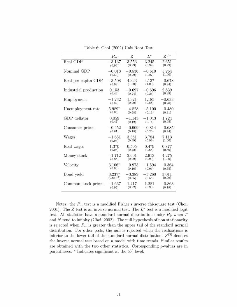
Table 6: Choi (2002) Unit Root Test

Pm Z L� Z(3)

Real GDP �3:137(0:99)

3:553(0:99)

3:245(0:99)

2:651(0:99)

Nominal GDP �0:013(0:50)

�0:536(0:29)

�0:610(0:27)

5:264(1:00)

Real per capita GDP �3:508(0:99)

4:323(1:00)

4:137(1:00)

�0:678(0:24)

Industrial production 0:153(0:43)

�0:697(0:24)

�0:696(0:24)

2:839(0:99)

Employment �1:232(0:89)

1:321(0:90)

1:185(0:88)

�0:633(0:26)

Unemployment rate 5:989�(0:00)

�4:828(0:68)

�5:100(0:16)

�0:480(0:31)

GDP de�ator 0:059(0:47)

�1:143(0:12)

�1:043(0:14)

1:724(0:95)

Consumer prices �0:452(0:67)

�0:909(0:18)

�0:814(0:20)

�0:685(0:24)

Wages �1:651(0:95)

3:381(0:99)

3:784(0:99)

7:113(1:00)

Real wages 1:370(0:08)

0:595(0:72)

0:479(0:68)

0:877(0:80)

Money stock �1:712(0:95)

2:601(0:99)

2:913(0:99)

4:275(1:00)

Velocity 3:106�(0:00)

�0:975(0:16)

�1:594(0:05)

�0:364(0:35)

Bond yield 3:237�(0:6e�3)

�3:389(0:35)

�3:260(0:55)

3:011(0:99)

Common stock prices �1:667(0:95)

1:417(0:92)

1:281(0:90)

�0:863(0:19)

Notes: the Pm test is a modi�ed Fisher�s inverse chi-square test (Choi,2001). The Z test is an inverse normal test. The L� test is a modi�ed logittest. All statistics have a standard normal distribution under H0 when Tand N tend to in�nity (Choi, 2002). The null hypothesis of non stationarityis rejected when Pm is greater than the upper tail of the standard normaldistribution. For other tests, the null is rejected when the realizations isinferior to the lower tail of the standard normal distribution. Z(3) denotesthe inverse normal test based on a model with time trends. Similar resultsare obtained with the two other statistics. Corresponding p-values are inparentheses. � Indicates signi�cant at the 5% level.

31

Table 7: Pesaran (2003) Unit Root Tests

� CIPS CIPS�

Lag length p p� 1 2 3 4 1

Real GDP 1 �2:070(0:12)

�1:793(0:46)

�1:708(0:48)

�1:609(0:71)

�2:309(0:15)

Nominal GDP 1 �2:261�(0:03)

�2:286(0:02)

� �2:573�(0:01)

�2:571�(0:01)

�2:261�(0:03)

Real per capita GDP 2 �1:848(0:37)

�1:823(0:41)

�1:911(0:29)

�1:773(0:48)

�1:848(0:37)

Industrial production 1 �2:105(0:10)

�1:804(0:44)

�1:781(0:48)

�1:793(0:46)

�2:105(0:10)

Employment 1 �1:748(0:53)

�1:383(0:92)

�1:613(0:70)

�1:493(0:83)

�1:748(0:53)

Unemployment rate 2 �2:700�(0:01)

�2:276(0:02)

� �2:150(0:07)

�2:299�(0:02)

�2:700�(0:01)

GDP de�ator 2 �2:293�(0:02)

�2:024(0:16)

�2:270(0:02)

� �2:194�(0:05)

�2:293�(0:02)

Consumer prices 2 �2:163(0:07)

�1:867(0:36)

�1:858(0:38)

�1:751(0:54)

�2:163(0:07)

Wages 2 �2:173(0:06)

�2:148(0:07)

�1:918(0:28)

�2:061(0:13)

�2:173(0:06)

Real wages 1 �2:325�(0:01)

�1:832(0:40)

�1:384(0:92)

�1:053(0:99)

�2:325�(0:01)

Money stock 1 �3:588�(0:01)

�2:226�(0:04)

�2:468�(0:01)

�2:180(0:06)

�2:656�(0:01)

Velocity 1 �2:980(0:01)

� �1:847(0:37)

�2:380�(0:01)

�2:412�(0:01)

�2:663�(0:01)

Bond yield 1 �2:774�(0:00)

�2:851�(0:00)

�3:254�(0:00)

�2:922�(0:00)

�2:774�(0:00)

Common stock prices 1 �2:855�(0:01)

�2:568�(0:01)

�2:251(0:08)

�2:001(0:25)

�2:855�(0:01)

Notes: CIPS is the mean of individual Cross sectionally augmentedADF statistics (CADF). CIPS� denotes the mean of truncated individualCADF statistics. The truncated statistics are reported only for one lagsince they are always equal to not truncated ones for higher lag lengths.Corresponding p-values are in parentheses. p� denotes the nearest integerof the mean of the individual lag lengths in ADF tests. � Indicates signi�cantat the 5% level.

32

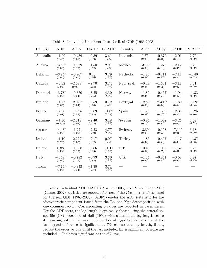
Table 8: Individual Unit Root Tests for Real GDP (1963-2003)

Country ADF ADFcbe CADF IV ADF Country ADF ADFcbe CADF IV ADF

Australia �1:69(0:42)

�0:439(0:51)

�0:59(0:89)

3:41(0:99)

Luxemb. 0:77(0:99)

�0:676(0:41)

�2:91(0:10)

2:75(0:99)

Austria �3:89�(0:00)

�1:379(0:15)

�1:50(0:62)

2:97(0:99)

Mexico �3:71�(0:00)

�1:270(0:18)

�2:12(0:35)

3:29(0:99)

Belgium �3:94�(0:00)

�0:207(0:60)

0:18(0:98)

3:29(0:99)

Netherla. �1:70(0:41)

�0:711(0:40)

�2:11(0:35)

�1:40(0:07)

Canada �2:92(0:05)

�2:689(0:00)

� �2:70(0:18)

3:24(0:99)

New Zeal. �0:48(0:88)

�1:531(0:11)

�3:11(0:07)

3:21(0:99)

Denmark �3:78�(0:00)

�0:370(0:54)

�3:25(0:05)

4:30(1:00)

Norway �1:85(0:34)

�0:457(0:50)

�1:94(0:42)

�1:33(0:09)

Finland �1:27(0:62)

�2:025�(0:04)

�2:59(0:18)

0:72(0:76)

Portugal �2:80(0:06)

�2:306�(0:02)

�1:80(0:49)

�1:69�(0:04)

France �2:66(0:08)

�0:395(0:53)

�0:89(0:82)

�1:69(0:04)

Spain �1:76(0:38)

�1:596(0:10)

�2:35(0:26)

�1:25(0:10)

Germany �1:96(0:302)

�2:219�(0:02)

�2:46(0:22)

3:18(0:99)

Sweden �0:94(0:76)

�1:092(0:24)

�3:25(0:05)

0:02(0:51)

Greece �4:43�(0:00)

�1:221(0:20)

�2:23(0:30)

4:77(1:00)

Switzer. �3:89�(0:00)

�0:158(0:62)

�7:11�(0:01)

3:18(0:99)

Iceland �1:10(0:70)

�2:222�(0:02)

�2:17(0:32)

0:07(0:53)

Turkey �1:86(0:34)

�0:407(0:53)

�1:47(0:63)

�1:37(0:08)

Ireland 0:88(0:99)

�1:358(0:15)

�0:86(0:83)

�1:11(0:13)

U.K. �0:45(0:89)

�1:050(0:25)

�1:52(0:61)

3:23(0:99)

Italy �4:58�(0:00)

�0:792(0:36)

�0:93(0:82)

3:30(0:99)

U.S. �1:34(0:60)

�0:841(0:34)

�0:58(0:90)

2:97(0:99)

Japan �7:74�(0:00)

�0:842(0:34)

�1:38(0:67)

3:71(0:99)

� � � �

Notes: Individual ADF, CADF (Pesaran, 2003) and IV non linear ADF(Chang, 2002) statistics are reported for each of the 25 countries of the panelfor the real GDP (1963-2003). ADFcbe denotes the ADF t-statistic for theidiosyncratic component issued from the Bai and Ng�s decomposition withone common factor. Corresponding p-values are reported in parentheses.For the ADF tests, the lag length is optimally chosen using the general-to-speci�c (GS) procedure of Hall (1994) with a maximum lag length set to4. Starting with some maximum number of lagged di¤erences and if thelast lagged di¤erence is signi�cant at 5%, choose that lag length, if not,reduce the order by one until the last included lag is signi�cant or none areincluded. � Indicates signi�cant at the 5% level.

33

Table 9: Chang (2002) Non Linear IV Unit Root Tests

SN statistics IGF1 IGF2 IGF3

Real GDP 8:365(1:00)

17:59(1:00)

16:48(1:00)

Nominal GDP �6:541�(0:00)

3:473(0:99)

4:126(1:00)

Real per capita GDP 12:88(1:00)

16:86(1:00)

14:52(1:00)

Industrial production 14:49(1:00)

17:98(1:00)

14:86(1:00)

Employment 5:297(1:00)

9:842(1:00)

7:671(1:00)

Unemployment rate �0:499(0:30)

4:958(1:00)

0:409(0:65)

GDP de�ator �5:179�(0:00)

4:090(1:00)

3:594(0:99)

Consumer prices �4:077�(0:00)

3:333(0:99)

5:049(1:00)

Wages �1:719�(0:04)

8:623(1:00)

6:167(1:00)

Real wages 10:84(1:00)

11:84(1:00)

8:631(1:00)

Money stock 1:911(0:97)

10:50(1:00)

11:08(1:00)

Velocity 2:696(0:99)

4:713(1:00)

3:312(0:99)

Bond yield �0:247(0:40)

0:918(0:82)

0:430(0:66)

Common stock prices 4:937(1:00)

5:894(1:00)

5:381(1:00)

Notes: The SN statistic corresponds to the average of individual non-linear IV t-ratio statistics (Chang, 2002). It has a N(0; 1) distributionunder H0. Three Instrument Generating Functions (IGF) are considered:IGF1(x) = x exp (�ci jxj) ; where ci 2 R is determined by ci = 3T�1=2i s�1 (�yit)where s2 (�yit) is the sample standard error of �yit: IGF2(x) = I(jxj < K)and IGF3(x) = I(jxj < K) � x ; where K is the second quantile of yi;t. �

Indicates signi�cant at the 5% level.

34

Table 10: Summary of Conclusions

Tests LLC IPS MW CH BNc BNi MP CH2 P IV

Real GDP I(0) I(0) I(0) I(0) I(1) I(0) I(0) I(1) I(1) I(1)

Nominal GDP I(0) I(1) I(0) I(0) I(1) I(0) I(0) I(1) I(0) I(1)

Real per capita GDP I(0) I(1) I(1) I(0) I(1) I(0) I(0) I(1) I(1) I(1)

Industrial production I(0) I(0) I(0) I(0) I(1) I(1) I(0) I(1) I(1) I(1)

Employment I(0) I(1) I(1) I(1) I(1) I(1) I(0) I(1) I(1) I(1)

Unemployment rate I(0) I(0) I(0) I(0) I(1) I(0) I(0) I(0) I(0) I(1)

GDP de�ator I(0) I(1) I(1) I(1) I(1) I(0) I(0) I(1) I(1) I(1)

Consumer prices I(0) I(1) I(1) I(1) I(1) I(1) I(0) I(1) I(1) I(1)

Wages I(0) I(0) I(0) I(0) I(1) I(0) I(1) I(1) I(1) I(1)

Real wages I(0) I(0) I(0) I(0) I(1) I(1) I(0) I(1) I(1) I(1)

Money stock I(0) I(0) I(0) I(0) I(1) I(0) I(0) I(1) I(0) I(1)

Velocity I(0) I(1) I(1) I(1) I(1) I(1) I(0) I(0) I(1) I(1)

Bond yield I(1) I(1) I(1) I(1) I(1) I(0) I(0) I(0) I(0) I(1)

Common stock prices I(1) I(1) I(1) I(1) I(1) I(1) I(0) I(1) I(0) I(1)

Notes: All results are obtained in a model with �xed e¤ects at the 5% level. LLCdenotes the Levin, Lin and Chu (2002) test (statistic t��); IPS denotes Im, Pesaran andShin (2003) test (statistic W ), MW denotes the Maddala and Wu (1999) test (statisticPMW ); CH denotes the Choi (2001) test (statistic ZMW ); BNc denotes the Bai and Ng(2004) test for common factors (ADF cF orMQ statistics), BNi denotes the Bai and Ng(2004) test for idiosyncratic shocks (statistic P ce ), MP denotes the Moon and Perron(2004) test (statistic t�a); CH2 denotes the Choi (2002) test (statistic Pm); P denotesthe Pesaran (2003) test (statistic CIPS with p = 2) and IV denotes the Chang (2002)test (statistic IGF2):

35