NBER WOREING PAPER SERIES

THE BEHAVIOR OF MONEY, CREDIT AND PRICESIN A REAL BUSINESS CYCLE

Robert G. King

Charles I. Plosser

Working Paper No. 853

NATIONAL BUREAU OF ECONOMIC RESEARCH1050 Massachusetts Avenue

Cambridge MA 02138

February 1982

University of Rochester, Department of Economics and GraduateSchool of Management respectively. A preliminary version of thispaper was presented at the Seminar on Monetary Theory and MonetaryPolicy, Konstanz, West Germany, June 1981. Robert Barro, HerschelGrossman, John Long, and Bennett McCallum provided useful feedbackon earlier drafts of this paper. We have also benefited from semi-nars at the University of Rochester, University of Chicago, andUniversity of Pennsylvania. King's participation in this researchis supported by the National Science Foundation under grant SES 8007513 and Plosser's by the Center for Research in Government Policyand Business. The research reported here is part of the NBER'sresearch program in Economic Fluctuations. The above individualsand institutions should not be regarded as necessarily endorsingthe views expressed in this paper.

NBER Working Paper #853february 1982

The Behavior of Money, Credit and Prices in a Real Business Cycle

ABSTRACT

This paper analyzes the interaction of money and the price level

with a business cycle that is fully real in origin, adopting a view

which differs sharply from traditional theories that assign a signifi-

cant causal influence to monetary movements. The theoretical analysis

focuses on a banking system that produces transaction. services on demand

and thus reflects market activity. Under one regime of baiik regulation

and fiat money supply by the monetary authority, the real business cycle

theory predicts that (i) movements in external monetary measures should

be uncorrelated with real activity and (ii) movements in internal mone-

tary measures should be positively correlated with real activity. Pre-

liminary empirical analysis provides general support for this focus on

the banking sector since much of the correlation between monetary

measures and real activity is apparently with inside money.

Robert G. KingCharles I. PlosserUniversity of RochesterRochester, NY 14627(716) -275-3895

I. INTRODUCTION -

The correlation between variations in the quantity of money and

fluctuations in real activity is perhaps the most discussed and least

easily explained element of macroeconomics. Traditional monetary theo-

ries of business fluctuations stress market failure as the key to under

standing this relationship, interpreting monetary movements as a primary

source of impulses to real activity

This paper describes an initial attempt to account for the relation—

ship between money and business cycles in terms that most economists would

label reverse causation. The basic idea is that the real sector drives the

monetary sector, in contrast to the traditional view of monetary movements

as business cycle impulses. In our model, variations in the real oppor-

tunities of the private economy--which include shifts in government

policies such as government purchases and tax rates, as well as technical

and environmental conlitions---are assumed to cause variations in both meas-

ures of real activity and monetary quantities The formal theoretical

framework involves two key elements: (i) market clearing determination

of prices and quantities and (ii) rational expectations based on accurate

knowledge of the current values of all pertinent state variables. Real

business cycles emerge in this setup as a result of the optimal plans of

private agents who are confronted by variations in real opportunities.

-2--

Since the idea that certain monetary quantities are endogenous is

an old one, it is useful to outline two recurrent themes. First, viewing

monetary services as a privately produced good, changes in internal money

can be systematically related to economic activity through the operation

of an unregulated banking sector.' Second, in a setting that contains a

mix of external (fiat) money and internal money, changes in external

money can be related to either economic activity or to the forces that

drive economic activity through central bank policy response. For example,

Tobin (1970) provides an earlier analysis of a model with endogenous money

that emphasizes central bank policy response. Tobints deterministic treat-

ment involves the Keynesian idea that money and real activity respond to

the same causal influence--aggregate demand.2

Our analysis, on the other hand, employs a stochastic neo-classical

growth model in which movements in money and real activity respond

to variations in real opportunities. The analysis focuses on the banking

system and draws heavily on another analysis of Tobin (1963) and the

important recent contribution by Fama (1980a). In the absence of central

bank policy response, the model predicts that movements in external money

measures should be uncorrelated with real activity. Some preliminary

empirical analysis (using annual data for the 1953-1978 period) provides

general support for our emphasis on private banks since the correlation

between monetary measures and real activity is primarily with inside

money.

-3-

Our motivation for pursuing this line of research is to produce an

equilibrium model that is capable of explaining the joint time series

behavior of real quantity variables, relative prices, the price level,

and alternative monetary measures. It is a common observation, however,

that such models must include a causal role for money [e.g., Lucas (l977)J.

Yet, economic theory has yet to provide a convincing rationale for such

a "nonneutrality" of money. Traditional explanations focus on central,

but implausible, market failures: Keynesian models most obviously so and

recent equilibrium theories in terms of the use of information, particu-

larly contemporaneous monetary information [(see King l98l)]. Consequently,

it seems worthwhile to consider alternative hypotheses concerning money and

business cycles.

The organization of the paper is as follows. In Section II we

describe a simple model that is capable of generating real business cycles.

This model is used to discuss correlations between an "internal" monetary

quantity and real activity. In Section III, with fiat money grafted

onto the model, we analyze the relationship between monetary quantities,

output, and the price level in an unregulated banking environment. The

analysis also deals with a regulated banking system where it becomes

crucial to spell out the form of central bank policy. In Section

IV we discuss some of the empirical implications of the theory

and provide a preliminary analysis of the post-war U.S. experience.

-4-

II. THE REAL ECONOMY

In this section a simple model economy is described that embodies the

potential for real business cycles. At this stage of research, government

is taken to exert no influence on the economy through tax policy or pur—

chases of final product. Rather, the model economy is driven solely by

shocks to current production opportunities that are assumed to have a

technological interpretation. Basically, the model is a stochastic growth

model with a single final product. Stochastic growth models of a more

general variety have recently been employed to study business cycles by

Long and Plosser (1980). Since such models incorporate many final products

and a more general pattern of production inter-relationships, richer

patterns of variation in economic activity can be generated. However,

the main aspects of the interactions of money, credit, and prices with

a real business cycle can be outlined in the present, simpler framework.

A. The Final Goods Industry

There is a single final product that can serve as either a consumption

good (x) or a capital good (k). This final product is produced by a constant

returns to scale production process that uses labor (n), capital (k), and

transaction services (d) as inputs. The output generated from given in-

puts is assumed to be uncertain due to stochastic technical factors.

The production technology is given by

(1) t+l = f(k> nyt,

-5-

where k is the amount of capital services, n is the amount of laboryt yt

services, and d is the amount of transaction services used in theyt

final goods industry.4 The production technology in (1) implies that

a unit of time corresponds to the production period for the single final

product.

Transaction services in (1) are viewed as an intermediate good

purchased by the final good producers from the financial industry (to

be described below). Although not involved directly in the production

of output in the same sense as labor and capital, transaction services

are taken to be a factor necessary to the firm's operation similar to

other organizational and control inputs. The final good industry and

financial industry could be vertically integrated so that transaction

services are provided by the firm internally. We believe, however,

that it is more fruitful to view firms specializing either in the

production of the final good or in the production of the transaction

5services.

The production process described by (1) is subject to two random

shocks, and dated by the time of their realization. For sim-

plicity, {) and {} are assumed to be strictly positive, mutually

uncorrelated {EC+5) = 0, for all t and s], stationary stochastic proc-

esses. Further, it is assumed that each process is serially independent

and that for all t,E(4) = E() = 1. The roles played by these two

shocks are quite different as will become clear in the discussions

-6-

that follow. At this point it is sufficient to recognize that alters

expected time t+l output and affects time t input decisions by altering

intertemporal opportunities. On the other hand, represents the

basic uncertainty of the production process by altering output in an

unexpected manner.6

Production is assumed to be under the supervision of N identical com-

petitive firms. Firms operate by selling claims against the future product

obtained by combining units of capital, labor, and transaction services

that are rented at their respective rental prices, w, and Each

firm is assumed to sell one unit of claim for each unit of output as de-

termined by f(k yt'This assumption amounts to a definition of

a "share" in the firm. The going market price of claims is v., so that

the firm faces a static maximization problem involving the choice of

inputs (kr. n, dyt) that maximizes profits, vf(kt dt) -Wtflyt

-

- The assumption of constant returns to scale implies that

the firm has a supply of claims that is horizontal at the price v.

How does this artifical economy correspond to the real world? So

far we have described firms that combine factors of production into

final goods. The firms rely on external finance to accomplish production

activity, issuing claims in the amount vf(nt k, and renting

the services of factors of production from their owners. Thus, the

economy has the counterparts of trade credit, or circulating capital

(shares), and physical capital that play key roles in many macroeconomic

theories [as described, for example, by Haberler (1963)].

-7-

B. Asset Returns

Within the model economy there are two basic ways for agents to

hold wealth--as claims to the ownership of the goods in process at the

firm (circulating capital) and as physical capital.

The commodity value at time t+l of each claim or share issued at

time t is simply so that the realized rate of return can be ex-

pressed as

-

= rVt yt

Given that is known at t and independent of the expected return

conditional on all information available at time t, is just

E(rytIt) = - 1

where it is assumed that is independent of I [i.e.,

E(t+iII) = E(t+i) = 1].

An alternative store of value is capital. The owner of a unit of

final product used as physical capital in period t earns a return

that involves two components. The first component involves the rental

rate paid in period t, and the second incorporates the capital de-

preciation rate 5. The net return to the capital owner is

__ - 1 r.

-8-

This return is certain in commodity terms because depreciation is not

random and rental prices are paid in period t.

It is useful in the analysis that follows to view agents as having the

opportunity to borrow or lend at a (real) riskless market interest rate, r.

Since these bonds are internal in character, in an economy of identical

individuals, the representative agent will not execute any such trans-

action. Nevertheless, the rate at which he/she would do so is well

defined and the rental rate on capital is fixed by the requirement

that the returns to these two assets be equalized. This follows from

the fact noted above that capital owners bear no risk. Thus, in

order for no arbitrage opportunities to exist, it must be the case

that = 1 - (l_)/(l-'-r).The claims to production, on the other hand, are uncertain due to

Thus, the yields on these claims, r, and the return to the real

bond need not be equalized. In the absence of production uncertainty

the "share price" v is simply 4/(l+r). More generally, however,

uncertainty leads agents to discount future income at a higher rate

resulting in a lower "share price."

C. The Financial Industry

The financial industry provides accounting services that facilitate

the exchange of goods. The accounting system of exchange [described by

Fama (l9SOa, pp. 42-43)] operates through bookkeeping entries that permit

indirect market transactions without necessarily requiring any physical

medium of exchange. The produced output of the financial industry is

-9-

transactions services and is an intermediate good. The production of

transaction services is assujied to be instantaneous with a nonstochastic

constant returns to scale production function,

(2) d = h(ndt,kd)

where, dt and kdt are the amounts of labor and capital services allocated

to the financial industry.8 A key element of this production structure is

that the production of the intermediate good requires a neglibible amount

of time relative to the production of the consumption/capital good. In

addition, the constant returns to scale structure implies that at given

factor prices, w and the financial industry has a supply curve that

is horizontal at p.t

So far we have described the real productive activities of

the financial industry--flows of services generated from factors of

production--in a manner that could describe any intermediate product.

The transaction (banking) industry, however, usually provides these

services in conjunction with portfolio management or intermediary

services. That is, the industry maintains claims on the probability

distribution of output ("loans") and issues other claims ("deposits").

At this stage of the analysis, however, households have no demand

for transactions services except indirectly through their demand for

the final product. Consequently, the scope for the portfolio manage-

ment role of banks is limited. More specifically, since households do

not hold "deposits," transfers of "funds" from firms to individuals in

—10-

payment for labor and capital services cannot be conducted through book-

keeping entries alone. Thus, some form of wealth must "change hands"

and we suppose that it is desirable that some "assets" actually be held

in the financial industry to facilitate these transfers. For example,

one can view firms as selling shares to individuals and depositing the

"proceeds" with the financial industry which then provides the accounting

and transaction services necessary in disbursing the factor payments to

households during the period. We further assume that the size of the

"deposit" can be represented as Ydt. indicating that it is proportional

to the flow of transaction services.9

The activities of the financial industry described above are quite

limited. In Section III, the role of the financial industry is expanded

by assuming households have an independent desire for transactions services.

In that environment, the financial industry becomes more easily identified

with a banking system. Nevertheless, the present setup is sufficiently

developed to highlight the relationship between real output fluctuations

and deposits in an economy that possesses no fiat money.

Consider, for example, the case of an autonomous movement in that

raises demand for all factors of production including transactions services

and thus deposits. (We assume that the increase is not reversed in equili-

brium by increases in the wage and rental rates.) A general strategy for

simplifying the structure of the model that is consistent with the above sto-

ry is to define the effective production function for the final goods producer

—11—

as f*(kt,nt), where and are the total quantities of capital and

labor used to produce final output (both directly and indirectly through

transactions services). The comparable "reduced form" production ex-

pression for deposits is h*(nt,kt). In the analysis below, the co-movement

of deposits with output emerges as a result of underlying movements in

total amounts of capital and labor inputs.

D. Equilibrium Prices and Quantities

To complete the specification of the model it is necessary to specify

the preferences of a representative agent and to discuss the nature of the

constraints that the economy places on his/her behavior.

The representative individual is assumed to be infinite lived and

possess the lifetime utility function,

(3) U u(x ., - n .)tj=O

t+j t+j

which involves a fixed utility discount factor () and a single period

utility function that depends only on consumption (x+) and leisure

- nt.), where n is the total hours available in each period. The

utility maximand is the expected utility measure EtUu(xt, fl - +

EtUt+i, where E denotes the conditional expectation based on full

information about economic conditions at time t.

Newly produced units of product, y = f*(n1, kti)cptit and capital

in place, =(1_6)kt_i, are assumed to be perfect substitutes in pro-

duction and consumption so that the economy as a whole faces the constraint,

—12-

(4) x + k � + kt

In this expression, k corresponds to the (per capita) amount of resources

allocated at date t to the final product and deposit industries (k = kyt+

10

'dt

One analytical mechanism for generating equilibrium quantities and

prices [see, for example, Lucas (1978) and Long and Plosser (1980)] is

the study of the planning problem for the representative agent. This

strategy exploits the optimality of a competitive equilibrium in envi-

ronments such as the present setup to calculate equilibrium quantities.

Furthermore, at optimal planned quantities, subjective and technical rates

of substitution correspond to competitive exchange rates.

From the point of view of the representative agent, the state of

the economy at date t is summarized by the values of two random variables,

St = yt + kt and The first represents a measure of "national wealth"

and the second represents a technical factor affecting the current oppor-

tunity to transfer resources intertemporally.

The "economic planner" faces the constraint that x + kt � s,

terms of sources and uses of current product. The recursive equation

of the planner's problem has the form

(5) J(St,ct) ={k?xnt}

- kt, fl - +

where = t_itf*t_i,kt_i) + (1 - 5)kti. Equation (5) also assumes

-13-

that the resource constraint holds as an equality (i.e., consumption is

a good). The first-order conditions, derived in Appendix B, can be writ-

ten as,

u1(s - k, n - n) = E{Ji(st+1, t+l+ (l-)]

+ +i+i -

and

u2(s - k, i - n) =

+ +i+i -

which emphasize two distinct features of individual behavior. The first

term on the right-hand side of these expressions measures variations in

the expected rewards to capital formation and work, respectively. The

second term involves the effects of production uncertainty on the house-

hold's assessment of the marginal value product of capital formation

and work, in the discussion that follows the latter pattern of effects

is de-emphasized by simply dropping the final term. This simplification

implies that the share price, v, equals t/(l+rt) and amounts to omitting

possibly interesting cyclical Variation in "risk premia." In focusing

on expected returns, however, the discussion is within the spirit of

much macroeconomic analysis.

The decision rules for this problem,k(s, ) and

n(s, &),

-14-

are stationary functions of the state variables, s In

the discussion below, it is assumed that the derivatives of the optimal

decision rules have the following signs and magnitudes:

<1 ,

dn dnt , t— >0 —>0

ds

(Explicit expressions for these derivatives are given in ppendix B).

The economic reasoning underlying these conditions is as follows. First,

an increase in the amount of the initial stock, s, involves additional

wealth so that the consumption of final product and leisure are expected

to rise. Agents, however, choose to spread some portion of this wealth

increment over time and do so by increasing the amount of commodity

dkallocated to capital services so that 0 < < 1. This raises

St

the marginal product of labor since capital and labor are complements in

production kn > 0). If the wealth effect on labor supplied, which

arises from the increased output of final goods next period, is out-

weighed by the increase in the real wage (marginal product of labor),

dn

then hours worked rises, > 0.

Second, an increase in involves both wealth and substitution

effects. Given current inputs, future production is higher and the

current returns to additional units of factors of production are higher.

—15-

These offsetting effects are analogous to the income and substitution

effects of a real interest rate change. Essentially, the small impact

on capital of a shift in 4, on the amount of output allocated to capital

dkservices 0, reflects the idea that the income and substitution effects

t

are roughly offsetting. On the other hand, the substitution effect of such

dnshifts on labor supply is presumed to dominate so that > 0.

E. Inside Money, Credit, and the Real Business Cycle

In the real business cycle described above, a positive correlation

(co-movement) of real production, credit, and "inside money" (created by

the financial services industry) arises from the general equilibrium of

production and consumption decisions by firms and households. The timing

patterns among these variables, however, depends on the source of the

variation in real output.

1. Unexpected Output Events ()

Real events of this form operate by altering the initial conditions, s,

pertinent for economic agents' plans for consumption, investment, and hours

of work. As discussed above, the implications of an unexpected wealth

increment ( > 1) for capital is straightforward: the economy responds

with higher net investment than would otherwise have been the case.

The implications for units of labor services are less clear, reflecting

the offsetting impact of higher national wealth and a higher marginal

product. Under the assumption that the wage effect dominates, real out-

put rises and exhibits positive serial correlation. During the course

-16-

of such an economic expansion the volume of credit is also high as

firms finance relatively large amounts of goods in process. Real rates

of return move in a countercyclical direction, as agents' opportunities

to spread wealth over time are subject to diminishing returns (since

total time is in fixed supply).

The movement in final goods production induces a higher volume

of financial services and an accompanying increase in real bank deposits

due to the role of financial services as an intermediate factor in prow

duction. Hence, the volume of "inside money" quantities are positively

correlated with output with a rough coincidence in timing.

At least some business cycle episodes, however, are commonly viewed

by outside observers as involving a substantially different timing pattern.

In particular, traditional business cycle analysts [Burns and Mitchell

(1946)]; modern time series macroeconometricians [Sims (1972, 1980)];12

and monetary historians [Friedman and Schwartz (1963)] view monetary

variables as "leading" measures of real activity, with various forms of

13timing concepts employed.

2. Expected Output Events ()

One way of generating a substantially different timing pattern is

through shifts in the interteniporal opportunities of the economy as a

whole. Real events of this form, represented by alter agents'

allocations of leisure and consumption between the present and the future

for a given level of national wealth. A positive shock (4 > 1), under

the assumptions outlined above, expands hours worked with little accom-

panying change in consumption or capital. The fact that financial services

are an intermediate product- -which can be produced more rapidly than the

final product-- leads to an expansion of the quantity of such services and of

—17--

bank deposits. Consequently, movements in hours worked, interest rates

and security prices, deposits/financial services, and trade credit all

occur prior to the expansion of output. The subsequent increment to

time t+l wealth (stemming from the joint impact of the exogenous shift,

and agents' responses to that shift) works much like the above

discussion of unexpected output events.

—18-

III. CURRENCY, DEPOSITS, AND PRICES

In order to investigate the relationship between nominal aggregates

and the real business cycle, it is necessary to augment the hypothetical

economy developed above. In this section, a non-interest bearing govern-

ment-supplied fiat currency (dollars, in a chauvinistic gesture) is

introduced and the factors affecting its value are analyzed.

First, in order for currency to be a well-defined economic good,

and thus, to have a determinate price in terms of a unit of output (l/P),

there must be a demand function for currency that reflects the economic

value assigned to the services of currency by economic agents. It would

be desirable to build in basic aspects of the economic environment that

give rise to a commodity money and then to examine the potential for

a non-backed governmental issue to haie positive value. This route,

however, is not attempted in the present paper. Instead, we assume that

households have a demand for transaction services. These services are

produced by combining units of currency purchasing power with the deposit

services of the banking industry. The production technology is

(6) =T(Ct, d1)

where is the flow of transactions services produced at time t,

is the stock of currency purchasing power, and dht is the quantity of

services purchased from the financial industry.

The demand for real transactions services is assumed to be a

positive function of the total market transactions that the household

-19-

engages jn, as well as depending negatively on the cost of producing

these services. This demand for real transactions services and the pro-

duction technology (6) imply a pair of derived demands for real currency

and services of the accounting system of exchange. These derived demands

are functions of the rental price of real currency, Rt/(l+Rt), arid the

effective cost of financial services, p. In forming these rental prices,

two important assumptions are made. First, there is a market for one

period nominal bonds that bear interest rate Rt. This nominal rate is

the sum of the real component, r, and an expected rate of inflation,

E().14

Second, if banks are required to hold noninterest bearing reserves,

the returns earned by depositors may not match market rates. Given the

proportionate link between financial services (dr) and deposits (Yd),

the effective cost of a unit of deposit services, p, is influenced by

this reserve regulation. In the absence of reserve requirements =Pt,

where is the rental price of deposit services in the competitive en-

vironment of Section II.

It is assumed that the real demands for currency and financial

services take the following forms,

(7a) c = "l+t ' ,

:t)

(Th) d = ' '

-20-

The + or - below the arurnents denote the signs of the partial derivative,

e.g., c/ay > 0. These assumptions about partial derivatives involve

some conventional assessments about the impacts of own and cross rental

price elasticities.

This formulation involves several ideas that are worth emphasizing.

First, the structure of the markets for currency and financial services

is analogous to that provided by Fama (1980a). In contrast to the dis-

cussion in Section II, the financial industry can now be viewed as

providing services that facilitate the exchange of goods through an

accounting system. As discussed previously, the accounting system

operates through bookkeeping entries without necessarily requiring

any physical medium of exchange. Following Fama (1980a), we assume that

it is desirable that some "assets" be held in the financial industry.

Thus, the financial industry holds claims (shares) on the probability

distribution of output and issues deposits.15 In the process of market

exchange, the claims that individuals and firms hold on the banks' port-

folio (deposits) are altered, with the banking system recording these

transfers. Banks pass on to depositors the return to the portfolio of

assets less a fee for services.

Second, the structure of the financial industry implies that the

direct cost of the bookkeeping services, does not hinge on the

character of the assets in the bank's portfolio. As discussed by Fama

(1980a), it follows that there is no particular reason that deposits

-21-

would be a homogenous good in an unregulated financial industry. Finally,

the idea that financial services and currency are substitutes, but not

perfect substitutes, is implicit in (7). In particular, currency yields

a real service flow in that there are some transactions (either of magni-

tude or character) that are more efficiently carried out using currency

rather than the accounting system of exchange.'6

Given the setup of the markets for currency and deposit servicesdescribed above, determinacy of the price level is insured if the

government fixes the nominal quantity of currency--direct or indirect

regulation of financial sector quantities and/or characteristics are

not necessary. Nevertheless, regulations can be important

for two reasons. First, regulations produce a differentiated class of

suppliers of financial services (banks) whose deposits are sometimes des-

cribed as inside money. Second, regulations can have influences on the

price level by altering the effective rental price of financial services.

The analysis below focuses on the implications of alternative

banking structures for the behavior of currency, deposits, and prices.

For clarity, the bulk of the discussion is conducted under the assunip-

tion that the treasury/central bank maintains a policy of controlling

the issue of nominal currency so that the stock of currency (C. = Ptct)is an exogenous random variable. Other models of central bank behavior

are discussed in Part B below.

A. Money and Prices--Unregulated Banking

In an unregulated banking environment we assume that the deposit industry

would hold virtually no currency. Consequently, the determination of the

—22-

price level involves the requirement that the real supply of currency (C/P)

be equal to the real demand for currency given by (7a) above. The equilibrium

price level is then

(8) Pt = C/2(.)

where 9(.) is the demand function for real currency. Using the arguments of

we can rewrite this condition as

(9) Pt = P(C, R,+ - + -

The signs of the respective derivatives in (9) are straightforward and

warrant little explanation.17

An important feature of (9) is that nominal demand deposits do not appear.

Thus, as stressed by Fama (l980a), there is no need for government control of

banking or the supply of deposits to insure a determinate price level. Banks,

in a competitive, unregulated environment, simply pass portfolio returns on

to their depositors less a fee charged for the provision of transactions

services, so that =

Although the signs of the partial derivations in (9) are straight-

forward, it is important to stress that we have ruled out real effects

of sustained increases in the growth of currency.18 Such behavior leads

to sustained inflation and a rise in the nominal interest rate, R, which

implies a fall in the demand for real currency and a rise in real deposits.

-23-

Since an increase in real deposit services involves the use of real resources,

the economy is made worse off by sustained inflation. We assume, however,

that this increase in the size of the financial sector has no important

implications for the real general equilibrium. It is not obvious that

this is a good assumption from an empirical point of view. Nevertheless, it

does serve to bring into sharp focus the distinction between "inside"

and "outside" money, particularly with respect to the neutrality and

superneutrality of government currency issue.

B. Money and Prices--Regulated Banking

In the unregulated environment the price level is determined in the

"currency market" and deposits play no essential role. There are a number

of bank regulations, however, that serve to distinguish banks from other

financial intermediaries. This section discusses the extent to which

these regulations alter the nature of price level determination. As it

turns out, the impact of regulations depends on (1) the interaction of

banking regulation with the external money supply policy of the central bank!

treasury and (ii) the extent to which government mandates can be off-

set by countervailing private substitutions.

1. Portfolio Regulations and Reserve Requirements

It is useful to start by discussing a set of regulations that do

not have any important consequences for the price level. Suppose that

the government specifies the "risk composition" of the underlying assets

against which deposits are claims. As long as agents can offset this

restriction by rebalancing the contents of their portfolios (i.e., the

distribution of total wealth between the banking sector and other portfolio

-24-

managers), then this regulation will have no impact on any real variables

or the price level.'9

On the other hand, restrictions specifying that banks must hold some

fraction (0) of their nominal asset portfolio in the form of noninterest

bearing reserves issued by the central bank may have important effects.

For example, the central bank could specify that reserve accounts are

deposits of securities, with nominal interest accruing to the central

bank. This mechanism is one way of imposing a deposit tax with the con-

sequence that the cost of deposit services would be > Such a

deposit tax results in a reduction in the size of the banking sector and

an increase in the real demand for currency.2° The impact of this reserve

requirement on price level determination depends on the central bank

policy. For example, if the treasury/central bank makes currency in the

hands of the public an exogenous quantity, unresponsive to developments

21 .in the banking sector, then the price level continues to be determined

by the requirement that the real stock of currency outstanding (Ct/Pt) be

equal to the real demand.

2. Alternative Central Bank Policies

The currency market determines the price level if the central bank

is assumed to make currency an exogenously controlled quantity. There

are, however, other control methods available to the central bank. For

example, if the central bank combines a reserve requirement with a policy

of controlling the sum of currency and nominal bank reserves (high powered

money), then the price level can be viewed as being determined in the

market for high powered money.

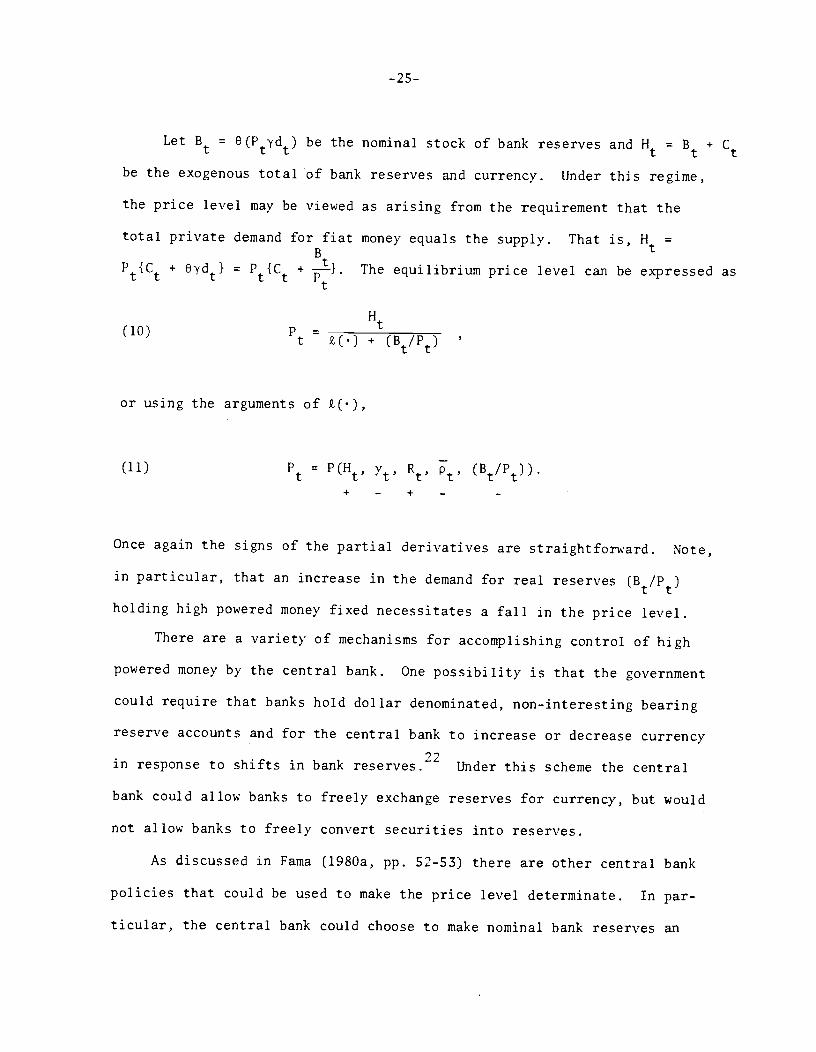
—25—

Let Bt = O(Pyd) be the nominal stock of bank reserves and Ht = B + Cbe the exogenous total of bank reserves and currency. Under this regime,

the price level may be viewed as arising from the requirement that the

total private demand for fiat money equals the supply. That is, Ht =B

+O'Yd}

= P{C + --}. The equilibrium price level can be expressed as

Ut(10) Pt - £(.) + (B/P)

or using the arguments of 2(.),

(11)Pt P(Ht, vt.' Rt, ' (Br/Pt)).

+ - + -

Once again the signs of the partial derivatives are straightforward. Note,

in particular, that an increase in the demand for real reserves(B/P)

holding high powered money fixed necessitates a fall in the price level.

There are a variety of mechanisms for accomplishing control of high

powered money by the central bank. One possibility is that the government

could require that banks hold dollar denominated, non-interesting bearing

reserve accounts and for the central bank to increase or decrease currency

in response to shifts in bank reserves.22 Under this scheme the central

bank could allow banks to freely exchange reserves for currency, but would

not allow banks to freely convert securities into reserves.

As discussed in Fama (1980a, pp. 52-53) there are other central bank

policies that could be used to make the price level determinate. In par-

ticular, the central bank could choose to make nominal bank reserves an

—26-

exogenous quantity and supply currency on demand. In this case (which

some argue are the current policies of the Federal Reserve), the price

level can be viewed as being determined in the market for reserves. The

equilibrium price level would be determined by the exogenous supply of

nominal reserves (Br) and the total real demand for deposit services.23

C. The Price Level and the Real Business Cycle

Price level movements in response to the two shocks and ) involve

two important factors. First, there is the impact of movements in real out-

put on the demand for outside money. Second, there is the impact of nominal

interest rates on the demand for outside money. Since variation in the

price level also depends on central bank policy, we focus on the case of

a regulated banking system with the central bank assumed to make the

quantity of high powered money exogenous.

It is convenient to summarize household and bank behavior in the

24following demand function for outside money

h =Pt

+ Xy-

iRt ,A > 0, > 0

where ht is the logarithm of high powered money, ' is the logarithm

of real output, Pt is the logarithm of the price level, and Rt is the

nominal interest rate. Using the fact that Rt = r + (EtPt+i-

and the monetary equilibrium condition that ht = h, it follows that a

rational expectations solution for the price level along the lines of

Sargent-Wallace (1975) can be written as

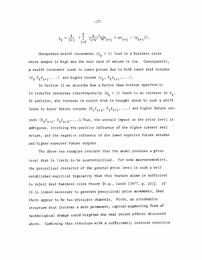
—27-

1 PjPt

= -i- jO EJht++ Pr+

- Ay.]}

Unexpected wealth increments > 1) lead to a business cycle

where output is high and the real rate of return is low. Consequently,

a wealth increment leads to lower prices due to both lower real returns

(r, Er+1 ) and higher income Etyt+lIn Section II we describe how a better than average opportunity

to transfer resources intertemporally ( > 1) leads to an increase in r.

In addition, the increase in wealth that is brought about by such a shift

leads to lower future returns (Er+1, Er+2 ) and higher future out-

puts (Eyt+i, Ey+2).Thus, the overall impact on the price level is

ambiguous, involving the positive influence of the higher current real

return, and the negative influence of the lower expected future returns

and higher expected future outputs.

The above two examples indicate that the model produces a price

level that is likely to be countercyclical. For some macroecononiists,

the procyclical character of the general price level is such a well

established empirical regularity that this feature alone is sufficient

to reject real business cycle theory [e.g., Lucas (1977, p. 20)]. If

it is indeed necessary to generate procyclical price movements, then

there appear to be two principle channels. First, an alternative

structure that involves a more permanent, capital_augmenting form of

technological change could heighten the real return effects discussed

above. Combining this structure with a sufficiently interest sensitive

—28-

demand for money could lead to procyclical prices. Second, policy

response to real activity also could generate procyclical price move-

ments.25 For example, a positive response of outside money creation

to output could lead to a positive correlation between prices and out-

put.

-29-

IV. EMPIRICAL ANALYSIS

The preceding sections describe a simple model economy with business

cycles that are completely real in origin. Nevertheless, correlations between

real activity and monetary measures arise from the operation of the banking

system and central bank policy responses. In this section, we discuss some

of the predictions that our model makes concerning the joint time series

behavior of output, monetary aggregates, rates of return, and the price

level. In addition, we discuss U. S. business cycle experience during the

post World War II period, providing some gross correlations that bear on

the potential relevance of our theoretical stories.

Before proceeding, it is useful to briefly consider general strategies

for investigating the empirical importance of 'real business cycle' theories

and to discuss how the present analysis of money and the price level could

be related to such investigations.

One empirical strategy is to attempt to isolate a group of ob-

servable real disturbances that provide an explanation of much of a

particular nation's business cycle experience, in the sense of delivering

a "good fit." Candidates for such real shocks include government purchase,

tax, and regulatory actions; changes in technological and environment con-

ditions; and movements in relative prices that are determined in a world

market. In pursuing this line of research, the goal is to provide a

direct substitute for the high explanatory power of monetary variables

in other business cycles studies [e.g., Friedman and Schwartz (1963)

and Barro (1981a)]. The natural extension would be to study the explanatory

-30-

power of such real factors for monetary variables and the price level. In

our framework, many of these real variables would be restricted to influence

monetary quantities (particularly, inside money) through their influence on

output and a small set of relative prices. In this sense, aspects of the

present type of monetary theory do provide meaningful restrictions on

the data.

Another approach is to treat the fundamental real shocks as unob-

servable and to focus on the interactions between sectors that arise

during business cycles; a strategy that is the empirical analogue of the

theoretical analysis of Long and Plosser (1980). Since a particular real

business cycle theory restricts own and cross serial correlation properties

of industry output and relative prices, this route can provide valuable in-

formation about the regular aspects of business cycles even though the

sources of shocks are not identified. Again, the principal testable re-

strictions of theorizing along the above lines would arise from the

restricted fashion that variations in production in other sectors were

allowed to influence developments in the monetary sector.

Unfortunately, analysis of monetary phenomena using either of these

strategies is not feasible given the state of real business cycle models.

Consequently, the present empirical investigation is limited to providing

some admittedly crude correlations among the variables suggested by the

theory.

A. Summary Statistics

Summary measures of the series to be discussed below are presented

in Table I. The data are annual--generally yearly averages--for

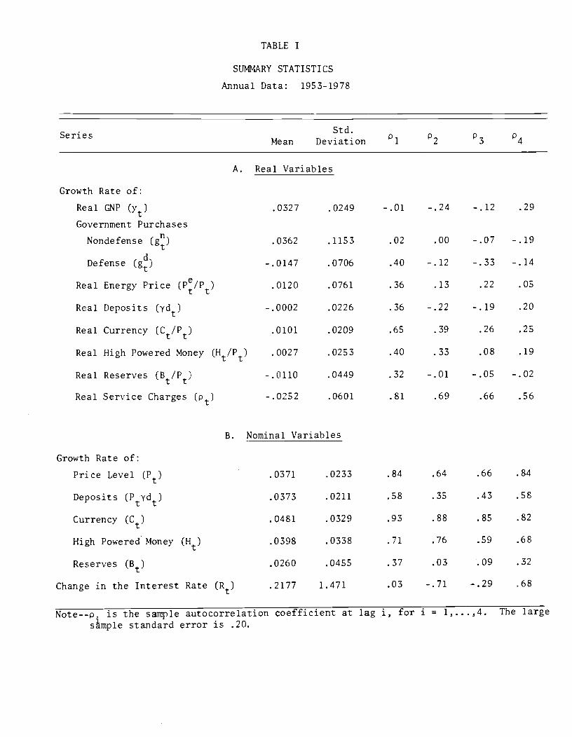
TABLE I

SUMMARY STATISTICS

Annual Data: 1953-1978

Std.Series

Mean Deviation 'l p2 p3 p4

A. Real Variables

Growth Rate of:

Real GNP (y) .0327 .0249 -.01 -.24 -.12 .29

Government Purchases

Nondefense (g) .0362 .1153 .02 .00 - .07 - .19

Defense (g) -.0147 .0706 .40 -.12 -.33 -.14

Real Energy Price .0120 .0761 .36 .13 .22 .05

Real Deposits (d) -.0002 .0226 .36 -.22 -.19 .20

Real Currency (Ct/Pt) .0101 .0209 .65 .39 .26 .25

Real High Powered Money (H/P) .0027 .0253 .40 .33 .08 .19

Real Reserves (B/P) - .0110 .0449 .32 -.01 - .05 - .02

Real Service Charges -.0252 .0601 .81 .69 .66 .56

B. Nominal Variables

Growth Rate of:

Price Level .0371 .0233 .84 .64 .66 .84

Deposits (PYd) .0373 .0211 .58 .35 .43 .58

Currency (Cr) .0481 .0329 .93 .88 .85 .82

High Powered Money (Ht) .0398 .0338 .71 .76 .59 .68

Reserves (Bt) .0260 .0455 .37 .03 .09 .32

Change in the Interest Rate (R) .2177 1.471 .03 -.71 -.29 .68

Note--p. is the sample autocorrelation coefficient at lag i, for i = 1,... ,4. The larges6ple standard error is .20.

-31-

the period 19531978.26 We focus on the 1953-1978 interval primarily to

avoid the period when the Federal Reserve maintained a policy of pegging

the yields on ii. S. government securities. The implications of such a

policy may be very different from those described in the previous section

where the central bank controls some measure of money.

The most noticeable feature in Table I is the different behavior of

nominal and real variables. Typically, the growth rates of real variables

display much less serial correlation than the growth rates of nominal

variables. For example, the growth of real demand deposits is much less

autocorrelated than the growth rate of nominal demand deposits. Indeed,

as previously noted by Nelson and Plosser (1982) and other authors, many

real variables display random walk like behavior in logarithmic form.

The most notable exceptions to this random walk behavior are real currency

(C/P) and real service charges both of which display significant

positive serial dependences.

B. Real Factors and Aggregate Output

As an example of how real factors could serve as important impulses

to business fluctuations, Table II reports regressions of aggregate output

on two components of government purchases of goods and services (real

federal defense and nondefense components) and the relative price of energy.

Table II indicates that defense purchases exert a positive influence on

output (though statistically a weak one) and that nondefense purchases are

unimportant. These results are consistent with Barrots (198lb) longer period

evidence that temporary increases in government purchases have an expansionary

TABLE II

REAL FACTORS AND OUTPUT GROWTH

Annual Data: 1953-1978

n d eny = + + Y2ng + y3tin(P/Pt) +

'yO 'l '2 Y3R2 s.e.(c) p1

.035** - .003 .097 .107* .191 .0239 -.04(.005) ( .045) (.073) ( .063)

Note--See Table I for the definition of the variables. LZn() in-

dicates the change in the logs of the variable. R2 is the coefficient

of determination, s.e.(c) is the standard error of the regression, p1

is the estimated first-order autocorrelation coefficient of the re-

siduals, which has a large sample standard error of .20, and standard

errors of the coefficients are in parentheses.

*Indicates significance at the 10% level.

**Indicates significance at the 5% level.

-32-

impact. Since our sample period involves only the Vietnam war, it is

perhaps not surprising that the t-statistic on defense purchases is low.

Table II also indicates a weak negative impact of the relative price of

energy. At present, we are seeking to augment these real factors with

other tax and expenditure measures. The main difficulty lies in con-

structing the average marginal tax rates that theory predicts would be

important in output determination.

Additional evidence on the importance of real disturbances in out-

put fluctuations is offered in Nelson and Plosser (1982). Using an

unobserved components model of output and the observed autocovariance

structure of real GNP, Nelson and Plosser conclude that real (non-monetary)

disturbances are the primary source of variance in real activity. This

result is based on the commonly held view that monetary disturbances should

have no permanent effects on real output and thus disturbances that are of

a permanent nature must be associated with real rather than monetary sources.

C. Money-Output Correlations

The theoretical model stresses that internal real monetary balances

should be positively correlated with real activity, since money is a pro-

duced input. Further, the model predicts that autonomous external nominal

money creation/destruction is neutral with respect to output growth. These

two ideas suggest the value of analyzing money-output correlations in two

forms: real versus nominal balances and internal versus external monetary

measures.

Table III presents some information on the contemporaneous relationships

between output growth and growth rates of alternative monetary measures.

TABLE III

CONTEMPORANEOUS MONEY-OUTPUT REGRESS IONS

Annual Data:

1953-1978

=

a0 +

cz1A

9nM

+

Equation

a0

Independent Variables (Mt)

Real Monetary Measures

Nominal Monetary Measures

Ydt

Ht/P

C/P

PYd

H

C

R2

s.e.(c)

P1

(1)

Ø33**

(.004)

740**

(.167)

.450

.0188

-.08

(2)

.031**

(.004)

.51O'

(.103)

.337

.0206

-.18

(3)

.025**

(.005)

.664**

(.202)

.311

.0211

- .01

(4)

.015

(.009)

.465**

(.222)

.155

.0233

.10

(5)

.026**

(.007)

.171

(.146)

.054

.0247

.00

(6)

.027**

(.009)

.111

(.153)

.022

.0251

.01

(7)

.025**

(.006)

.742**

(.161)

.176*

(.108)

.507

.0182

-.11

(8)

.023**

(.006)

.784**

(.162)

.194*

(.111)

.514

.0181

-.08

(9)

.017*

(.010)

.558*

-.080

(.326)

(.203)

.161

.0238

.10

(10)

.015

(.010)

.661**

.181

(.307)

(.197)

.185

.0234

.07

Note--See Table II for definitions and explanations of entries.

—33-

Equation (1) shows the strong, positive contemporaneous correlation that

exists between real demand deposits and economic activity. This strong

contemporaneous correlation is shared by real external balances measured

as currency or as high powered money (equations (2) and (3)). In nominal

balance form, equations (4), (5), and (6) show demand deposits are more

strongly correlated with real activity than either of the nominal external

money measures.

Further, (7) and (8) indicate that nominal high powered money and

currency growth have a positive partial correlation with output given real

demand deposits although the correlation is not as strong as that with

real deposits (either in terms of the magnitude of the coefficient or the

pertinent t-statistic).

From the standpoint of our theoretical discussion, the key aspects of

these contemporaneous correlations are as follows. First, the fact that

much of the correlation is with internal monetary measures is consistent

with our general view of the relationship between money and real activity.

Second, the fact that nominal money measures may be positively correlated

with real activity is at odds with our theory if the monetary authority

makes nominal monetary measures such as currency or high powered money

evolve in an autonomous manner.

To provide some further information on the relationship between output

growth and growth rates of alternative monies, Table IV reports some

analogous regression results that incorporate lags of the alternative

monetary measures.

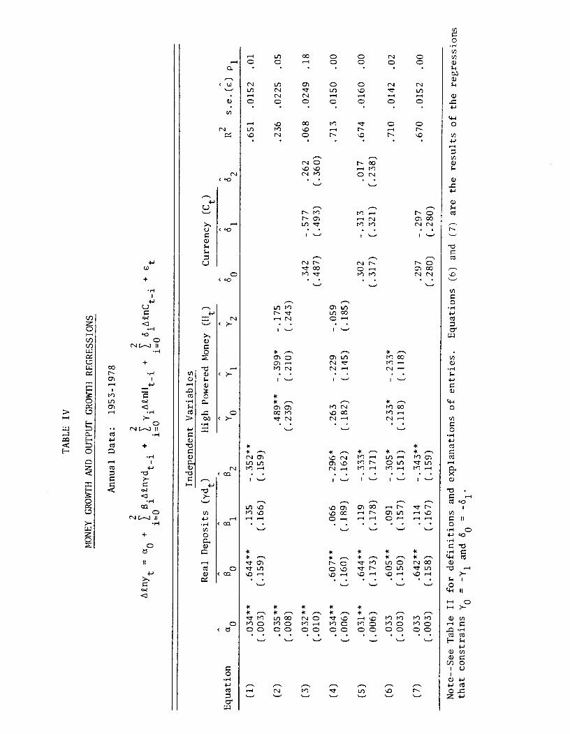
TABLE IV

MONEY GROWTH AND OUTPUT GROWTH REGRESSIONS

Annual Data:

1953-1978

2

2

2

= a0

+

.A9n

yd

+

+

ó.M

nC.

+

E

i=0

i=0

i=0

Equation

ac

Independent Variables

Real Deposits (Yd)

High Powered Money

2

(Ht)

Currency (Cr)

R

s.e.(c) p1

2

(1)

.034**

(.003)

.644**

(.159)

.135

(.166)

(.159)

.651

.0152

.01

(2)

.035**

(.008)

.489** 399*

(.239)

(.210)

-.175

(.243)

.236

.0225

.05

(3)

.032**

(.010)

.342

(.487)

-.577

(.493)

.262

(.360)

.068

.0249

.18

(4)

.034**

(.006)

.607**

(.160)

.066

(.189)

(.162)

.263

-.229

(.182)

(.145)

-.059

(.185)

.713

.0150

.00

(5)

.031**

(.006)

.644**

(.173)

.119

(.178)

(.171)

.302

(.317)

-.313

(.321)

.017

(.238)

.674

.0160

.00

(6)

.033

(.003)

.605**

(.150)

.091

(.157)

(.151)

.233*

(.118)

(.118)

.710

.0142

.02

(7)

.033

(.003)

.642**

(.158)

.114

(.167)

(.159)

.297

(.280)

-.297

(.280)

.670

.0152

.00

Note--See Table II for definitions and explanations of entries.

Equations (6) and (7) are the results of the regressions

that constrains

= -1

and 6o

=

—34-

Equation (1) in Table IV shows the results of adding two years of lagged

real deposits to the output regression. The F statistic pertinent for evalu-

ating the marginal contribution of these lags is 2.48, which is well below

the 95% critical value of 3.49, so that there is no strong evidence that

these lags are important. Equations (2) and (3) show analogous results for

nominal money growth measures.

In order to investigate the extent to which nominal money growth is

correlated with real activity, after accounting for real deposit growth,

equations (4) and (5) must be examined. The contemporaneous and two lags

of high powered money and currency in the hands of the public are not

important explanatory variables (the 95% critical value for F(3, 17) is

3.20 and the F statistics for the lags of high powered money and currency

terms are 1.22 and .40, respectively). However, the estimated coefficient

on current and lagged high powered money are opposite in sign and nearly

identical in magnitude, so that the change in high powered money growth appears

to be positively correlated with real activity (see equation (6)).

Overall, our interpretation is that the correlations reported in Tables

III and IV indicate that much of the relationship between money and fluctua-

tions in real activity is apparently with inside money, which is comforting

given the key role that the banking system plays in our theoretical story.

Nevertheless, somewhat weaker correlations between real activity and nominal

outside money may exist, suggesting it probably is necessary to analyze

policy response in greater detail for 1953-1978 period.

D. Money-Inflation Correlations

The theoretical model predicts that variations in external money, real

-35-

activity, the nominal interest rate and a measure of the cost of banking

services should be important in explaining movements in the price level.

Table V provides estimates of the price level equations (9) and (11) of

Section III under the assumption that a log-linear functional form is

appropriate. Although the nominal interest rate is endogenous and the

above discussion indicates that high powered money and/or currency may

also be endogenous due to policy response, ordinary least squares methods

are employed. Since there is a substantial empirical literature on

price level/money demand equations, our discussion focuses principally

on new aspects that are raised by the theoretical discussion above.

First, the theory suggests that a measure of external money, such as

currency a high powered money, is the relevant nominal aggregrate for price

level determination Farna (l980b) stresses this point] . Table V reports

results for both currency and high powered money.

Second, in the regulated banking environment described in Section III,

the relevant cost of deposit services (denoted involves both the direct

cost of providing an accounting system of exchange (denoted and the

interest that the bank/depositor must forego due to reserve requirements.

The empirical counterpart to the nominal unit cost of deposit services that

we have constructed is the ratio of total services charges on demand deposits

at Federal Reserve member banks to total check clearings by the Federal

Reserve. Deflating this measure by the price level leads to a measure of

real costs of deposit services, entered in Table V as p. However, during

some portions of the period under study, banks faced apparently binding

constraints on the level of interest payments that could be paid on demand

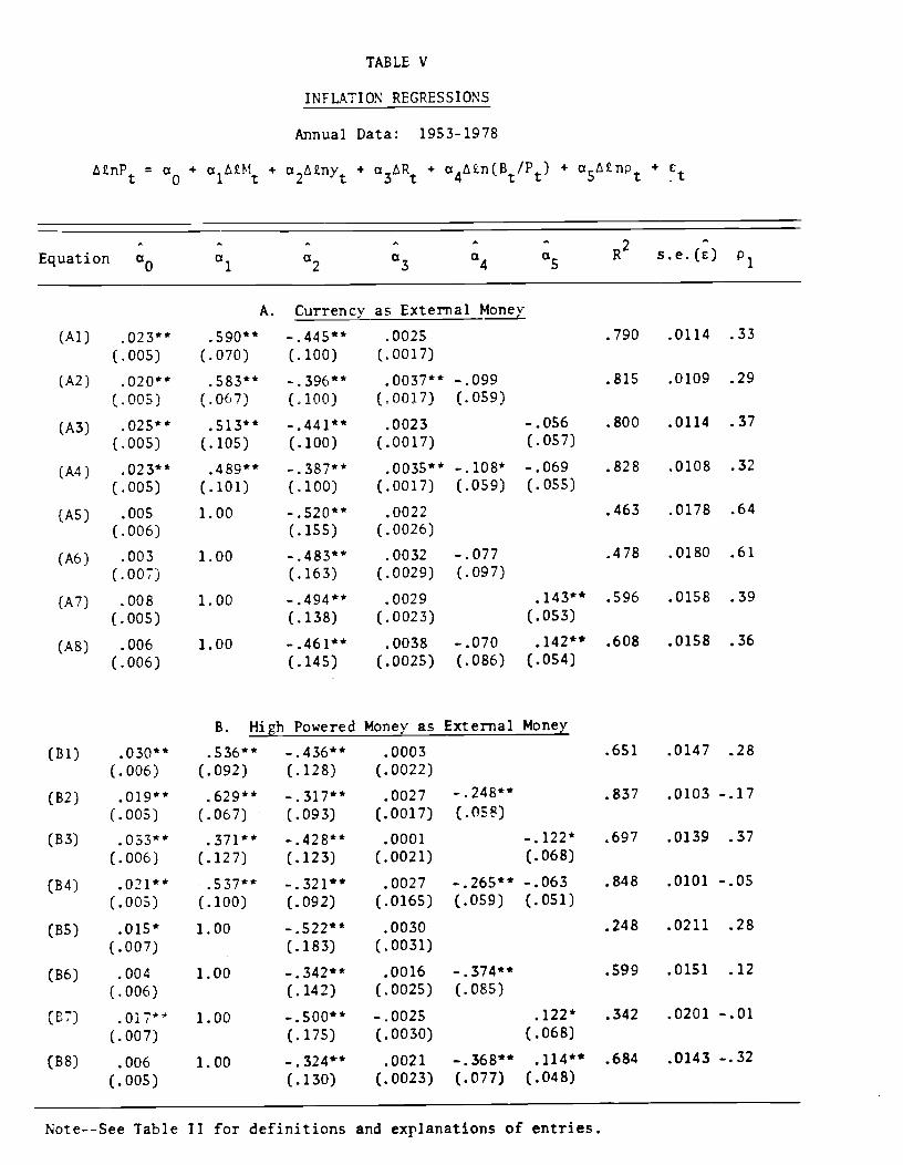
TABLE V

INFL&TION REGRESSIONS

Annual Data: 1953-1978

= + + a2TI)1 + a3tR + cI4f9.n(B/Pt)+ a&EnP +

Ct

Equation a0 a2a a

a5R2 s.e.(c) P1

A. Currency as External Money

(Al) .023** .590** _445** .0025 .790 .0114 .33

(.005) (.070) (.100) (.0017)

(A2) .020** 553** 396** .0037** -.099 .815 .0109 .29

(.005) (.067) (.100) (.0017) (.059)

(A3) .025** .513** _.441** .0023 - .056 .800 .0114 .37

(.005) (.105) (.100) (.0017) (.057)

(A4) .023** .489** - .387** .0035** _.108* -.069 .828 .0108 .32

(.005) (.101) (.100) (.0017) (.059) (.055)

(A5) .005 1.00 _.520** .0022 .463 .0178 .64

(.006) (.155) (.0026)

(A6) .003 1.00 _.483** .0032 -.077 .478 .0180 .61

(.007) (.163) (.0029) (.097)

(A7) .008 1.00 - 494** .0029 .143** .596 .0158 .39

(.005) (.138) (.0023) (.053)

(AS) .006 1.00 - .461** .0038 —.070 .142** .608 .0158 .36

(.006) (.145) (.0025) (.086) (.054)

B. High Powered Money as External Money

(Bi) .030** .536** - .436** .0003 .651 .0147 .28(.006) (.092) (.128) (.0022)

(B2) .019 .629** -. 317** .0027 _.248** .837 .0103 —.17

(.005) (.067) (.093) (.0017) (.058)

(B3) .033** .371** _.428** .0001 _.122* .697 .0139 .37

(.006) (.127) (.123) (.0021) (.068)

(B4) .021** 537** -. 321** .0027 _.265** —.063 .848 .0101 -.05

(.005) (.100) (.092) (.0165) (.059) (.051)

(B5) .015* 1.00 _.522** .0030 .248 .0211 .28

(.007) (.183) (.0031)

(B6) .004 1.00 _.342** .0016 _•374** .599 .0151 .12

(.006) (.142) (.0025) (.085)

(E7) .017** 1.00 -..S00 -.0025 .122* .342 .0201 -.01

(.007) (.175) (.0030) (.068)

(B8) .006 1.00 _.324** .0021 ..368** .114** .684 .0143 —.32

(.005) (.130) (.0023) (.077) (.048)

Note--See Table II for definitions and explanations of entries.

- 36-

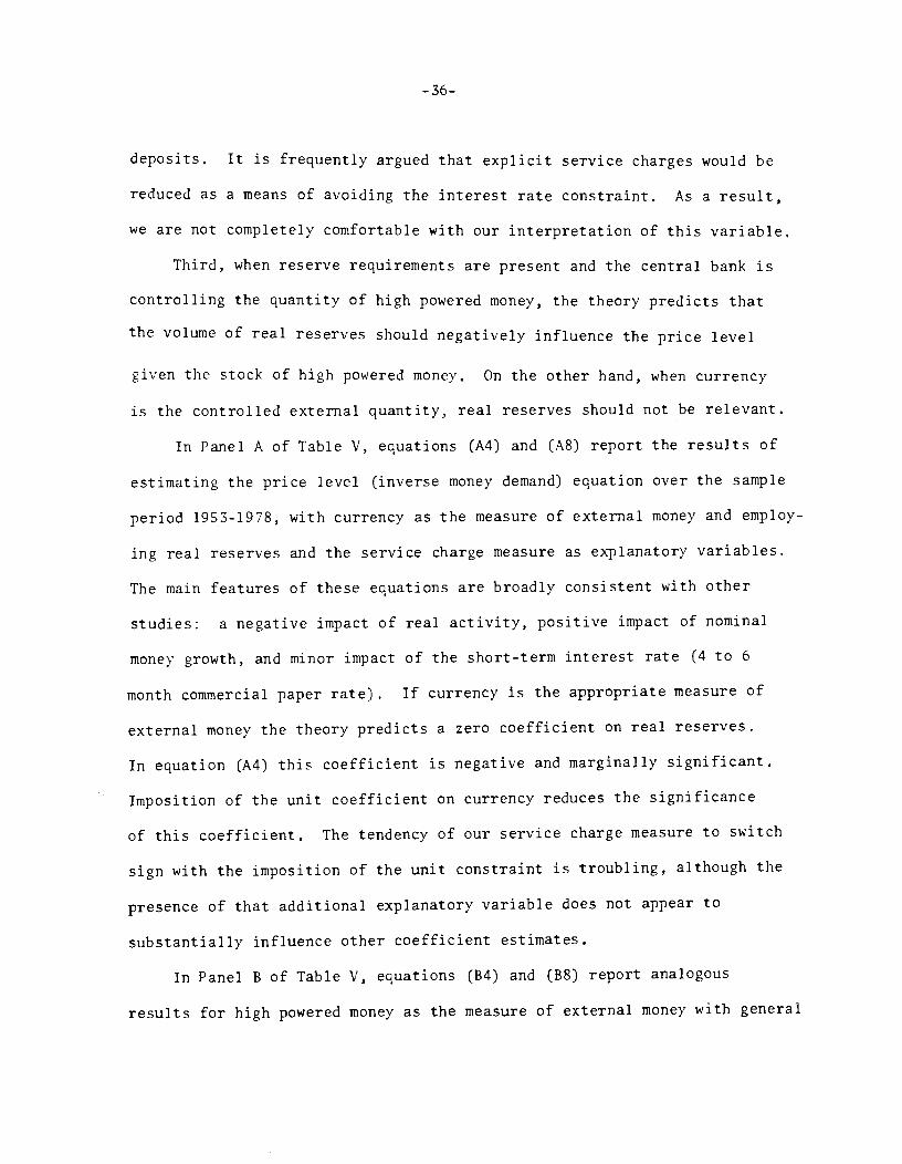
deposits. It is frequently argued that explicit service charges would be

reduced as a means of avoiding the interest rate constraint. As a result,

we are not completely comfortable with our interpretation of this variable.

Third, when reserve requirements are present and the central bank is

controlling the quantity of high powered money, the theory predicts that

the volume of real reserves should negatively influence the price level

given the stock of high powered money. On the other hand, when currency

is the controlled external quantity, real reserves should not be relevant.

In Panel A of Table V, equations (A4) and (A8) report the results of

estimating the price level (inverse money demand) equation over the sample

period 1953-1978, with currency as the measure of external money and employ-

ing real reserves and the service charge measure as explanatory variables.

The main features of these equations are broadly consistent with other

studies: a negative impact of real activity, positive impact of nominal

money growth, and minor impact of the short-term interest rate (4 to 6

month commercial paper rate), If currency is the appropriate measure of

external money the theory predicts a zero coefficient on real reserves.

In equation (A4) this coefficient is negative and marginally significant.

Imposition of the unit coefficient on currency reduces the significance

of this coefficient, The tendency of our service charge measure to switch

sign with the imposition of the unit constraint is troubling, although the

presence of that additional explanatory variable does not appear to

substantially influence other coefficient estimates.

In Panel B of Table V, equations (B4) and (B8) report analogous

results for high powered money as the measure of external money with general

-37-

features that are again broadly consistent with other studies. Under our

theory, real bank reserves should enter negatively in such price level

equations if high powered money is the controlled measure of external

money. This is borne out by significant negative coefficients in both

the unconstrained equation (B4) and constrained equation (B8). As pre-

viously, the service charge variable has a tendency to change sign when

the unit constraint is imposed.

Overall, the results of Table V are broadly consistent with the

theoretical stories told in the sections above. The negative influence

of real reserves on the price level potentially is important, both in

terms of explaining post-war price level behavior and, potentially, in

explaining the apparently anornolous behavior of the price level during

the interwar period. Finally, additional work needs to be done in pro-

ducing measures of the market prices of bank services.

-38-

CONG LUS IONS

This paper describes an initial attempt to account for the relation-

ship between money, inflation, and economic activity within the framework

of real business cycle theory. Although the empirical work presented

above is simplistic, we draw two main lessons from it. First, much of

the contemporaneous correlation of economic activity and money is appar-

ently with inside money, with inflation principally resulting from changes

in the stock of fiat money and variations in real activity. Second,

future work along these lines may have to consider policy responses that

are broad enough to produce variations in outside money that are contempo-

raneously correlated with real activity.

A main component of our future work in this area will be to develop

the implications of the analysis for security returns, so that the gen-

eral equilibrium predictions for these variables can be exploited in

tests of the model. This topic is especially important because Sims

(1980) and Fama (1981) have provided some hints about the interactions

of money, asset returns, and real activity. In addition, we

are in the process of casting the predictionsof theory within the class

of linear multivariate time series models so that broader patterns of

policy response can be examined and the results compared to other

studies. Thus, we feel there is a substantial amount of work to be

done.

In conclusion, it seems worthwhile to discuss two recurrent comments

on this line of research that we have received. First, there has been a

-39-

surprising willingness on the part of the many individuals to simultane-

ously argue that our model (a real business cycle model with an explicit

banking sector and central bank) is probably observationally equivalent

to existing theories and that a "common sense" view leads one to prefer

alternative models as descriptions of reality.27 This line of argument

puzzles us, since it was presumably on empirical grounds that the pro-

fession rejected pre-Keynesian "equilibrium theories" of the business

cycle that stressed real causes of economic fluctuations.

Second, some individuals have argued that market failure is

central to both the understanding of cyclical fluctuations and the primary

reason for economists to study these phenomena. Our view is that wide-

spread market failure need not be a necessary component of a theory of

business fluctuations and we (at least) remain interested in real business

cycle theory as potentially an important contribution to positive economics.

This perspective, however, is not inconsistent with the view that the

accumulation of scientific knowledge may lead to the design of more

desirable governmental policies toward business fluctuations (such as

tax and expenditure policies) or toward the regulation of the financial

sector.

Footnotes

1. A related story involves the operation of a commodity money economy

where changes in the production of the commodity money are related

to economic activity through variations in the relative price of

the commodity money.

2. Black (1972) also describes a model where both internal and external

money are endogenously determined.

3. Not surprisingly, this single sentence dismissal of received doctrine

on the relationship between money and business cycles has provoked a

sharp reaction from a number of readers. Although a footnote is not

an appropriate vehicle for a survey of contemporary macro theory,

some additional comments are perhaps in order. Keynesian models

typically rely on implausible wage rigidities, from the textbook

reliance on exogenous values to recent, more sophisticated efforts

of Fischer (1977) and Phelps and Taylor (1977) that rely on existing

nominal contracts. As Barro (1977) points out, a key feature of the

Fischer-Phelps--Taylor model is that agents select contracts that do

not fully exploit potential gains from trade. In addition, Azariadis's

(1978) micro-based model of wage-employment contracts implies that

perceived monetary disturbances do not alter output.

Recent analyses of monetary nonneutrality that stress expectation

errors based on "imperfect information" [Lucas (1977) provides a summary

of this viewpoint] similarly rely on an apparent failure in the market

for information. For example, information on monetary statistics is

cheap and readily available. King (1981) demonstrates that in Lucas'

(1973) model, real output should be .mcorre1ated with contemporaneously

available monetary information. Boschen and Grossman (1982) empirically

investigate this proposition and find that it is rejected by the data.

4. Capital services are measured in commodity units allocated to pro-duction at time t, labor services are hours worked, and transaction

services can be viewed as the number of bookkeeping entries used

(described more fully below).

5. An interesting and useful discussion of the role of money as a

factor of production can be found in Fischer (1974).

6. The multiplicative nature of the randomness in total production

implies a technological neutrality of the shocks with respect to

individual factors of production. A more general specification

might allow different stochastic elements to be associated with

particular factors of production. Such a model could provide a

richer set of co-movements among various measures of economic

activity.

7. In a certainty steady state--where real rates of return must be

equal to the subjective rate of time preference (a) and there are

no shocks ( = = 1)--the above definitions imply that

(k* * d*)}V -l+a q -

1+a l+cx k '

That is, the requirement that production takes time means that the

rental price of capital involves the marginal product of capital,

which influences output next period, discounted at the rate a.

8. We assume that transaction services are produced deterministically

for several reasons. The first reason is to keep the model as simple

as possible by limiting the number of independent sources of random

fluctuation. The second reason involves the assumption that sto-

chastic variations in transaction services are "small" in that they

have little impact on the real equilibrium in the final good industry.

It may, however, prove interesting to allow stochastic variation

in the provision of financial services as an independent source

of shocks to the real system. One might then proceed to decompose

real fluctuations into those attributable to shocks to the final

goods industry and the financial industry.

9. Assuming that transaction services and the stock of deposits are

related by a positive constant (any positive function is sufficient

for our purposes) implicity rules out firms (and in Section III,

individuals) using a given stock of deposits more or less intensively

(i.e., getting varying amounts of bookkeeping entries from a given

stock of deposits). We recognize that this is a strong assumption

(although it is commonly used in specifying production functions)

but it (over?) simplifies the analytical tractability of the model.

10. The details of household and firm optimization and equilibrium

conditions are discussed in Appendix A.

11. The sign of these terms is a function of the contemporaneous

covariance of J1 and . Assuming and are positively

correlated and is concave (J11 < 0), this covariance is

negative.

12. Sims (1980) discusses reverse causation of money and output work-

ing through central bank operating policies. The present setup

is a first step toward the type of small scale general equilibrium

model that is necessary to evaluate the reverse causation argument.

13. We deliberately employ the idea of a "leading variable" in a loose

manner so as to capture the common elements of these alternative

discussions. Sargent (1979, pp. 247-248) discusses how the timing

concepts employed by business cycle forecasters and time series

econometricians differ, relating a particular formal definition

of a 'leading indicator" to "causality" in the sense of Granger,

Sims, and Weiner,

14. At this point we note that we are ignoring any "risk premium" due

to inflation risk in our definition of the nominal rate.

15. Deposits in an unregulated environment are obviously not riskless

assets and banks would preumab1y offer deposits (claims on an

underlying portfolio of assets) with varying levels of risk

depending on demand.

16. It is also worth noting that consumers and producers are treated

asymmetrically in that the demand for real currency is only a

household demand and is not partly a derived demand by firms.

This reflects our view of the type of transactions that are

accomplished with cash and also a desire tQ keep the model

as simple as possible.

17. Although our model is similar in some respects o Black (1972),

our view of price level determination is quite different. In

Black's model, the price level is exogenous to the money supply

process. Equilibrium requires that the central bank supply fiat

currency on demand (passively) or else it loses economic value

as a medium of exchange.

18, In other words, our model is "super neutral," in the language of

monetary growth theory. It is worthwhile pointing out that this

literature does not provide a clearcut guide to the nature of

departures from super neutrality. For example, Tobin (1965),

has argued that an increase in inflation will lower real rates

of return and raise capital formation, by lowering the real value

of money and, consequently, raising saving. By contrast, Stockman

(1982) argues that inflation acts as a tax on the saving process

(in which money is an input) and, hence, depresses capital formation.

19. This application of the Modigliani-Miller theorem requires us to

ignore transactions costs in a specific manner that is stronger

than usual. In particular, the cost of running the accounting

system of exchange must be the same across regulated and unregulated

systems.

20. We are assuming that the reduction in the size of the deposit industry

has a negligible impact on the real general equilibrium of the model

(in particular, on the final goods production, which enters as a scale

variable in the demand for currency).

21. The central bank, therefore, "passively supplies" any quantity of

reserves required by the banking system.

22. Another possibility is to require banks to hold cash directly, For

the current discussion, however, it is not necessary to distinguish

between those operating schemes.

23. We have not analyzed the implications for price level determination

when the central bank attempts to control the interest rate. However,

this may be important for some periods in order to conduct an appro-

priate empirical investigation,

24. For simplicity, we ignore movements in the cost of deposit services

as an important factor affecting the price level,

25. Recent work using post-World War II data [e.g., Hodrick and Prescott,

(1980)] seems to suggest that the positive correlation between

output and price level movements may be not as robust as sometimes

thought.

26. Data sources are as follows: Real GNP, government purchase variab1es

and the GNP deflator are taken from The National Income and Product

Accounts of The United States 1929-1974 and various issues of the

Survey of Current Business. Currency in the hands of the public,

demand deposits, and bank reserves are from Business Statistics 1979.

High powered money is the sum of currency in the hands of the public

and bank reserves. The interest rate is the 4 to 6 month prime

commercial paper rate taken from Banking and Monetary Statistics

1941-1970 and various issues of the Annual Statistical Digest.

The energy price variable is the fuels, power, and related products

component of the Producer Price Index and is taken from Business

Statistics 1979. Finally the service charge variable is the

ratio of total service charges on demand deposits accrued by

Federal Reserve member banks to total check clearings by the

Federal Reserve. Both series are taken from Banking and Monetary

Statistics 1941-1970 and various issues of the Annual Statistical

Digest.

27. Grossman (1982) makes an explicit statement of this view.

References

Annual Statistical Digest, (various issues), Washington, D. C., Boardof Governors of the Federal Reserve System.

Azariadis, C., "Escalator Clauses and the Allocation of Cyclical Risks,"Journal of Economic Theory, 18, 1978, 119-155.

Banking and Monetary Statistics 1941-1970, Washington, D. C., Board ofGovernors of the Federal Reserve System, 1976.

Barro, R. J., "Unanticipated Money Growth and Economic Activity in theU. S.," Chapter 5 in Money, Expectations, and Business Cycles,Academic Press, New York, 1981a.

____________ "Output Effects of Government Purchases," Journal ofPolitical Economy, 89, December 198lb, 1086-1121.

____________ "Long Term Contracting, Sticky Prices and Monetary Policy,"Journal of Monetary Economics, 3, July 1977, 305-316.

Black, F., "Active and Passive Monetary Policy in a Neo-Classical Model,"Journal of Finance, 27, September 1972, 801-814.

Boschen, J. and H. I. Grossman, "Tests of Equilibrium Macroeconomics

Using Contemporaneous Monetary Information," forthcoming Journalof Monetary Economics, 1982. —

Burns, A. and W. Mitchell, Measuring Business Cycles, National Bureau ofEconomic Research, New York, 1946.

Business Statistics, 1979, Washington, D. C.: U.S. Department of Commerce1979.

Fama, E., "Banking in the Theory of Finance," Journal of Monetary Economics,6, January 1980a, 39-57.

____________ "Inflation, Output and Money," Working Paper, University ofChicago, May 1980b. -

___________ "Stock Returns, Real Activity, Inflation, and Money,"American Economic Review, 71, September 1981, 545-565.

Fischer, S., "Money and the Production Function," Economic Inquiry, 13,December 1974, 517-533.

__________—, "Long-Term Contracts, Ratiqnal Expectations, and the OptimalMoney Supply Role," Journal of Political Economy," 85, February 1977,191-205.

Friedman, M. and A. Schwartz, A Monetary History of the United States,National Bureau of Economic Research, Princeton University Press:Princeton, 1963.

Grossman, H. I., "Review of James Tobin's Asset Accumulation and Economic

Activity," forthcoming Journal of Monetary Economics, 1982.

Haberler, C., Prosperity arid Depression, 4th Edition, Atheneum: NewYork, 1963.

Hodrick, R. and E. Prescott, "Post-War U. S. Business Cycles: An

Empirical Investigation," Working Paper, Carnegie-Mellon University,November 1980.

King, R. G., "Monetary Information and Monetary Neutrality," Journal ofMonetary Economics, 7, March 1981, 195-206.

Long, J. B. and C. I. Plosser, "Real Business Cycles, Working Paper,University of Rochester, November 1980.

Lucas, R. E., "Some International Evidence on Output-Inflation Tradeoffs,"American Economic Review, 63, June 1973, 326-334.

____________ "Understanding Business Cycles," in Stabilization of theDomestic and International Economy, (eds. K. Brunner and A. Meltzer),Carnegie-Rochester Series in Public Policy, North Holland: Amsterdam1977, 7-29.

____________ "Asset Prices in an Exchange Economy," Econometrica, 46,December 1978, 1429-1448.

____________ "Methods and Problems in Business Cycle Theory," Journal

of Money, Credit, and Banking, 12, November 1980, 696-715.

National Income and Product Accounts of the U. S. 1929-1974, Washington,D. C.: U. S. Department of Commerce.

Nelson, C. R. and C. I. Plosser, "Trends and Random Walks in MacroeconomicTime Series: Some Evidence and Implications," forthcoming Journal ofMonetary Economics, 1982.

Phelps, E. S. and J. B. Taylor, "Stabilizing Power of Monetary Policy under

Rational Expectations," Journal of Political Economy, 85, February 1977,163-190.

Sargent, T., and N. Wallace, "Rational Expectations, the Optimal MonetaryInstrument and the Optimal Money Supply Rule," Journal of Political

Economy, 83, April 1975, 241-254.

Sargent, T., Macroeconomic Theory, Academic Press: New York, 1979.

Sims, C., "Money, Income, and Causality," American Economic Review,62, September 1972, 540-552.

___________ "Comparisonof Interwar and Postwar Business Cycles:Monetarism Reconsidered," American Economic Review, 70, May1980, 250-27.

Stockirian, A. C., "Anticipated Inflation and the Capital Stock in aCash-in-Advance Economy," forthcoming Journal of Monetary Economics,1982.

Tobin, J., "Commercial Banks as Creators of 'Money", 1963, reprintedas Chapter 16 of Essays in Economics, Volume 1: Macroeconomics,North Holland: Amsterdam, 1971.

____________ "Money and Income: Post Hoc Ergo Propter Hoc?", 1970,reprinted as Chapter 24 of Essays in Economics, Volume 1:economics, North Holland: Amsterdam, 1971.

____________ "Money and Economic Growth," 1965, reprinted as Chapter 9of Essays in Economics, Volume 1: Macroeconomics, North Holland:Amsterdam, 1971.

APPENDIX A

Market Behavior

The discussion in the text focuses almost entirely on the planning

problem and it may be worthwhile to discuss some aspects of economic

agents' market behavior in this hypothetical economy. The present

appendix dicussses the choice problems faced by households and firms

as well as the conditions of market equilibrium.

Household Optimization

The agent under study chooses current flows of consumption (xt)

and leisure (fin), as well as purchases/sales of real bonds (be), claims

to circulating capital (ar), and physical capital (kr) so as to maximize the

expected value of lifetime utility. The agent is assumed to view the

prices , v, q and w as functions of aggregate state variables

but not of his/her owii actions and, further, to employ the objective

probability distributions of these aggregate random variables in

forming expectations.

Wealth at date t is z btl + 41a1 + (l_o)ki.The recursive equation of the pertinent discrete time dynamic

programming problem is

H(z, l+ w)

= max[u(x, fi_n) + SEtH {z+i, l+r1 v1, w+1.}]

{x, i' b. a, k}

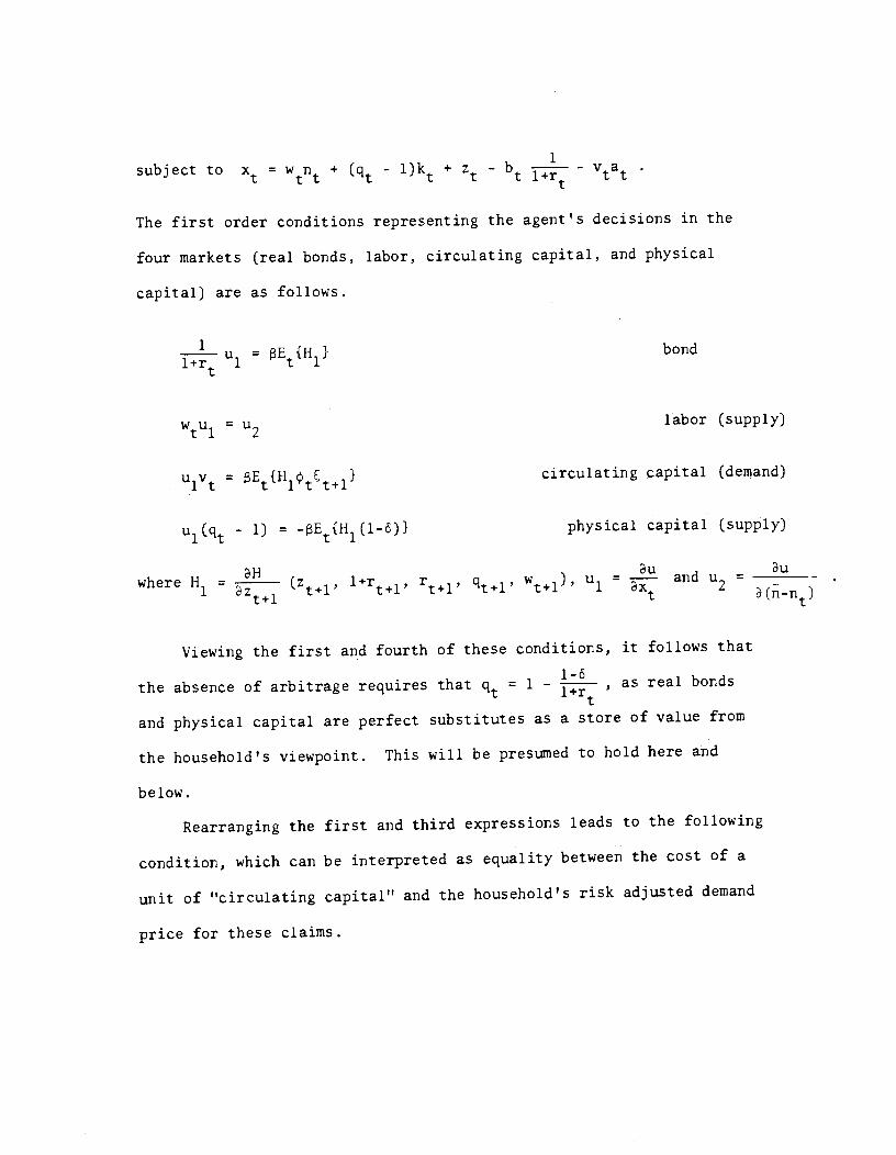
subject to x = Wfl + - l)kt + - bt- va

The first order conditions representing the agent's decisions in the

four markets (real bonds, labor, circulating capital, and physical

capital) are as follows.

u1 = EHi} bond

wu1 = u2labor (supply)

u1v. = circulating capital (demand)

u1(q - 1) = .E{H1(l_o)} physical capital (supply)

where H1 = a1 (z+i, l+ri r+i +1i w+i), u1 = and u2 =

Viewing the first and fourth of these conditions, it follows that

the absence of arbitrage requires that = 1 - , as real bonds

and physical capital are perfect substitutes as a store of value from

the household's viewpoint. This will be presumed to hold here and

below.

Rearranging the first and third expressions leads to the following

condition, which can be interpreted as equality between the cost of a

unit of "circulating capital" and the household's risk adjusted demand

price for these claims.

— , E{Hi(1 — l)}V l+r +

E{H1}

From an application of the envelope theorem, it follows that

=u1

so that H1 = u1(x1, - n) . Hence, it follows that H11 < 0.

Using this fact, it is straightforward that E{H1(t+i - 1)) <

E{Hi}E{+i - 1)) = 0, so that a household requires a risk premium --

in the sense of a lower share price and a higher expected return -- to

hold any specified positive quantity of circulating capital. In the

absence of uncertainty about future returns (e.g., has a degenerate

4tdistribution at its mean of unity), however, it follows that v = l+ri.e., the security price is simply the present value of the certain

future earnings.

The first two conditions simply involve efficient selection of an

intertemporal consumption—saving plan at interest rate r and a con—

temporaneous allocation between labor and leisure, i.e., a labor supply

decision.

Firm Optimization

Following the production example above, it simplifies matters to

"vertically integrate" the final product and financial industries so

that there is a single production decision being made, based on a pro-

duction function of the firm, = tt+if*(nt, kr).

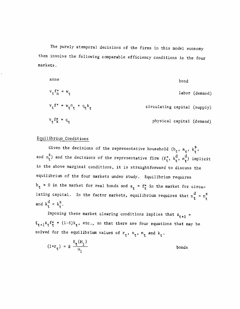
The purely atemporal decisions of the firms in this model economy

then involve the following comparable efficiency conditions in the four

markets.

none bond

vf = w labor (demand)

vtf* = wn + qk circulating capital (supply)

vf = physical capital (demand)

Equilibrium Conditions

Given the decisions of the representative household(br, a, k,

and n) and the decisions of the representative firm(f, k, n) implicit

in the above marginal conditions, it is straightforward to discuss the

equilibrium of the four markets under study. Equilibrium requires

= 0 in the market for real bonds and a = f in the market for circu-

lating capital. In the factor markets, equilibrium requires that n =nand kd kS.

t t

Imposing these market clearing conditions implies that =

+ (l_5)kt, etc., so that there are four equations that may be

solved for the equilibrium values of r. '' and kt.

E{H }(l+r) = bondsU1

*V f (Ti , k)u1 =

U2 labortn t

2 Et{Hi(+1 - 1)))

circulating capital+ ____________Vt

=

l+r Et{Hi}

1—cS

Vtf(fl, k) = 1 - l+r physical capitalt

where H1 is evaluated at equilibrium values, i.e.,

H ( q f* + (l-6)k, v1, w1) where1 t+ltt t

1 +rt +1

q4 and w1 satisfy updated versions of the above

four conditions.

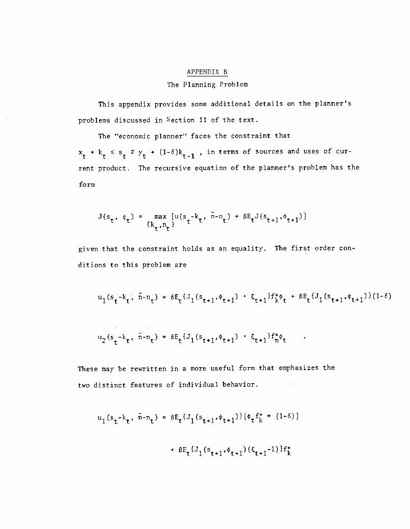
APPENDIX B

The Planning Problem

This appendix provides some additional details on the planner's

problems discussed in Section II of the text.

The "economic planner" faces the constraint that

x + � + (1_S)ki , in terms of sources and uses of cur-

rent product. The recursive equation of the planner's problem has the

form

J(s, q) = max [u(s_kt n-np + 8EtJ(s+i,I+i)]

given that the constraint holds as an equality. The first order con-

ditions to this problem are

ui(s_kti= +

u2(s_k, n = +lThese may be rewritten in a more useful form that emphasizes the

two distinct features of individual behavior.

ui(s_kt,= + (l-ô)]

+

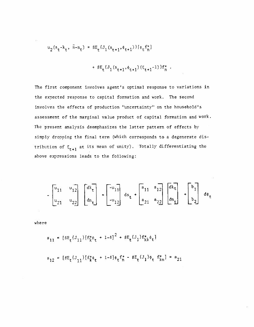
u2(s_k, nt) =

+

The first component involves agent's optimal response to variations in

the expected response to capital formation and work. The second

involves the effects of production "uncertainty" on the household's

assessment of the marginal value product of capital formation and work.

The present analysis deemphasizes the latter pattern of effects by

simply dropping the final term (which corresponds to a degenerate dis—

tribution of tl at its mean of unity). Totally differentiating the

above expressions leads to the following:

[ u [ak r-u raii {k [b- I I I I

=I I ds + I I I

+I I

[2l u2j LtJ Lii [2l a2j [nJ L'D2J

where

a11 = t3l1 kt ++

a12 — + l_6)f - E{Ji} f] = a21

a22 = ]2 + E{Ji} f*4]

b1 = [{J} f*[f*i + 1-] + 8E{J1}f]

b2 = + 8F {J1) f]

Solving this system leads to the following set of expressions for

the derivatives of the "policy functions" k(s ) andn(st,

where = (u1 +a11)(u22

+a22)

-(U12 + a12)(u2 +

a21) is positive.

= 1{u11u22-

u12)2 (a22u11 + u12a12))

dk= {b2(u21 +

a21)-

b1(u22-

a22))

=A{a11u12

-a12u11}

= 1{b1(u12 +a12)

-b2(u11

+a11))

The discussion in the main text, assumes that these derivatives

have the following signs and magnitudes:

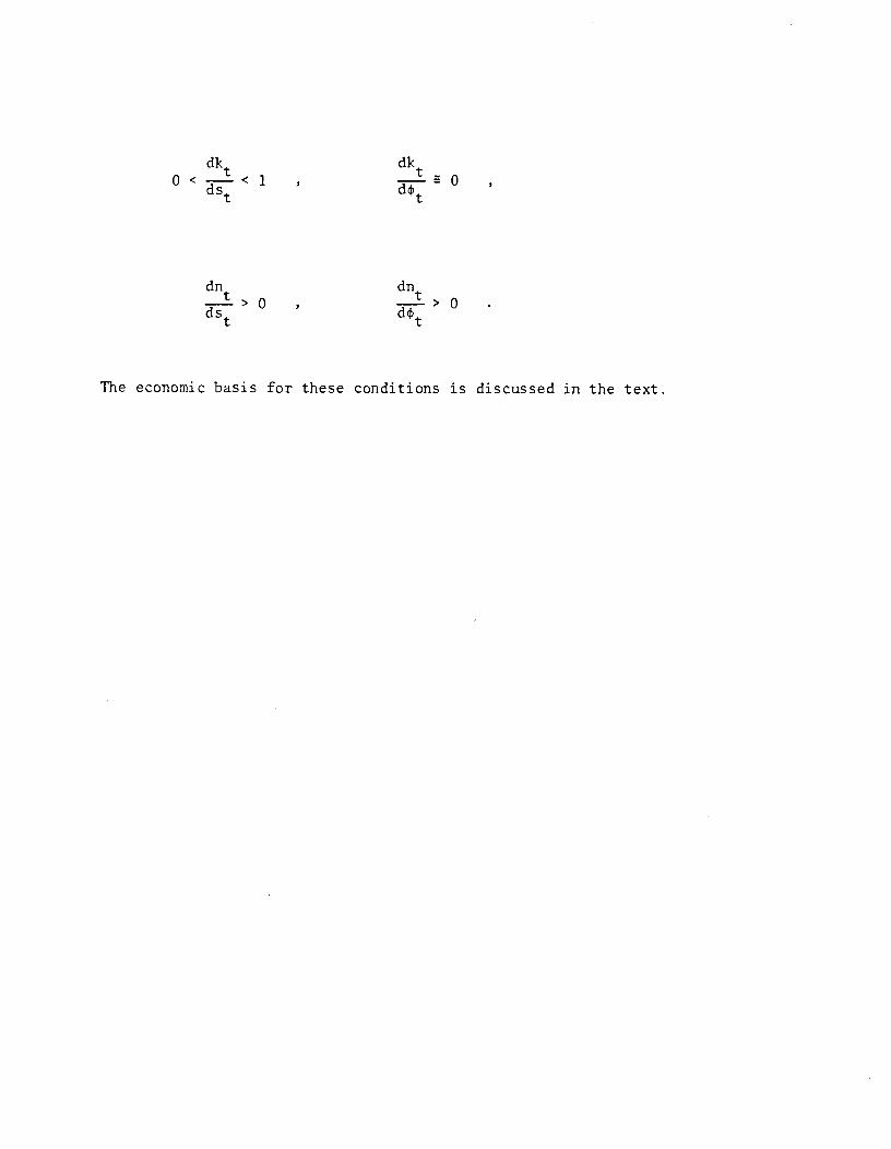
dk dk1

ds

dn dn—->o —.-->ods dt

The economic basis for these conditions is discussed in the text.