Embed Size (px)
Citation preview
WHAT GOODS DO COUNTRIES TRADE?NEW RICARDIAN PREDICTIONS
ARNAUD COSTINOT AND IVANA KOMUNJER
Abstract. Though one of the pillars of the theory of international trade, the extreme
predictions of the Ricardian model have made it unsuitable for empirical purposes. A sem-
inal contribution of Eaton and Kortum (2002) is to demonstrate that random productivity
shocks are su¢ cient to make the Ricardian model empirically relevant. While successful at
explaining trade volumes, their model remains silent with regards to one important ques-
tion: What goods do countries trade? Our main contribution is to generalize their approach
and provide an empirically meaningful answer to this question.
Date: June 2007.A¢ liations and Contact information. Costinot: Department of Economics, University of California at San
Diego, [email protected]; Komunjer: Department of Economics, University of California at San Diego,
Acknowledgments: We thank Gene Grossman, Gordon Hanson, Jim Rauch, Bob Staiger and seminar
participants at UC Davis, UC Irvine, Penn State, and UC San Diego for very helpful comments. Nadege
Plesier provided excellent research assistance.1
2
1. Introduction
Though one of the pillars of the theory of international trade, the extreme predictions
of the Ricardian model have made it unsuitable for empirical purposes. As Leamer and
Levinsohn (1995) point out: �The Ricardian link between trade patterns and relative labor
costs is much too sharp to be found in any real data set.�
A seminal contribution of Eaton and Kortum (2002) is to demonstrate that random pro-
ductivity shocks are su¢ cient to make the Ricardian model empirically relevant. When
drawn from an extreme value distribution, these shocks imply a gravity-like equation in a
Ricardian framework with a continuum of goods, transport costs, and more than two coun-
tries. While successful at explaining trade volumes, their model remains silent with regards
to one important question: What goods do countries trade? Our main contribution is to
generalize their approach and provide an empirically meaningful answer to this question.
Section 2 describes the model. We consider an economy with one factor of production,
labor, and multiple products, each available in many varieties. There are constant returns
to scale in the production of each variety. The key assumption of our model is that labor
productivity may be separated into: a deterministic component, which is country and in-
dustry speci�c; and a stochastic component, randomly drawn across countries, industries,
and varieties. The former, to which we refer as �fundamental productivity�, captures factors
such as climate, infrastructure, and institutions that a¤ect the productivity of all producers
in a given country and industry.1 The latter, by contrast, re�ects idiosyncratic di¤erences in
technological know-how across varieties.
Section 3 derives our predictions on the pattern of trade. Because of random productivity
shocks, we can no longer predict trade �ows in each variety. Yet, by assuming that each
product comes in a large number of varieties, we generate sharp predictions at the industry
level. In particular, we show that, for any pair of exporters, the ranking of the ratios of their
fundamental productivity levels fully determines their relative export performance across
industries. Compared to the standard Ricardian model� see e.g. Dornbusch, Fischer, and
1Acemoglu, Antras, and Helpman (2007), Costinot (2006), Cuñat and Melitz (2006), Levchenko (2007),
Matsuyama (2005), Nunn (2007), and Vogel (2007) explicitly model the impact of various institutional
features� e.g. labor market �exibility, the quality of contract enforcement, or credit market imperfections�
on labor productivity across countries and industries.
NEW RICARDIAN PREDICTIONS 3
Samuelson (1977)� our predictions hold under fairly general assumptions on transport costs,
the number of industries, and the number of countries.2 Moreover, they do not imply the
full specialization of countries in a given set of industries.
Section 4 investigates how well our model squares with the empirical evidence. We consider
linear regressions tightly connected to our theoretical framework. Using OECD trade and
labor productivity data from 1988 to 2003, we �nd fairly strong support for our new Ricardian
predictions: countries do tend to export relatively more (towards any importing country) in
sectors where they are relatively more productive.
Our paper contributes to the previous trade literature in two ways. First, it contributes to
the theory of comparative advantage. Our model generates clear predictions on the pattern
of trade in environments� with both multiple countries and industries� where the standard
Ricardian model loses most of its intuitive content; see e.g. Jones (1961) and Wilson (1980).
Our approach mirrors Deardor¤ (1980) who shows how the law of comparative advantage
may remain valid, under standard assumptions, when stated in terms of correlations be-
tween vectors of trade and autarky prices. In this paper, we weaken the standard Ricardian
assumptions� the �chain of comparative advantage�will only hold in terms of �rst-order
stochastic dominance� and derive a deterministic relationship between exports and labor
productivity across industries.
Second, our paper contributes to the empirical literature on international specialization,
including the previous �tests� of the Ricardian model; see e.g. MacDougall (1951), Stern
(1962), Balassa (1963), and more recently Golub and Hsieh (2000). While empirically suc-
cessful, these tests have long been criticized for their lack of theoretical foundations; see
Bhagwati (1964). Our model provides such foundations. Since it does not predict full inter-
national specialization, we do not have to focus on ad-hoc measures of export performance.
Instead, we may use the theory to pin down explicitly what the dependent variable in cross-
industry regressions ought to be.
As we discuss later in the paper, our model also provides an alternative theoretical under-
pinning of cross-industry regressions when labor is not the only factor of production. The
validity of these regressions usually depends on strong assumptions on either demand� see
2Deardor¤ (2005) reviews the failures of simple models of comparative advantage at predicting the pattern
of trade in economies with more than two goods and two countries.
4 COSTINOT AND KOMUNJER
e.g. Petri (1980) and the voluminous gravity literature based on Armington�s preferences�
or the structure of transport costs� see e.g. Harrigan (1997), Romalis (2004), and Morrow
(2006). One of the main messages of our paper is that many of these assumptions can be
relaxed, as long as there are stochastic productivity di¤erences within each industry.
2. The Model
We consider a world economy comprising i = 1; :::; I countries and one factor of production�
labor. There are k = 1; :::; K products and constant returns to scale in the production of each
product. Labor is perfectly mobile across industries and immobile across countries. The wage
of workers in country i is denoted wi. Up to this point, this is a standard Ricardian model.
We generalize this model by introducing random productivity shocks. Following Eaton and
Kortum (2002), we assume that each product k may come in Nk varieties ! = 1; :::; Nk, and
denote aki (!) the constant unit labor requirements for the production of the !th variety of
product k in country i. Our �rst assumption is that:
A1. For all countries i, products k, and their varieties !
(1) ln aki (!) = ln aki + u
ki (!);
where aki > 0 and uki (!) is a random variable drawn independently for each triplet (i; k; !)
from a continuous distribution F (�) such that: E[uki (!)] = 0.
We interpret aki as a measure of the fundamental productivity of country i in sector k
and uki (!) as a random productivity shock. The former, which can be estimated using
aggregate data, captures cross-country and cross-industry heterogeneity. It re�ects factors
such as climate, infrastructure, and institutions that a¤ect the productivity of all producers
in a given country and industry. Random productivity shocks, on the other hand, capture
intra-industry heterogeneity. They re�ect idiosyncratic di¤erences in technological know-how
across varieties, which are assumed to be drawn independently from a unique distribution
F (�). In our setup, cross-country and cross-industry variations in the distribution of produc-tivity levels derive from variations in a single parameter: aki .
Assumption A1 generalizes Eaton and Kortum�s (2002) approach along two dimensions.
First, it introduces the existence of exogenous productivity di¤erences across industries. This
will allow us to shift the indeterminacy in trade in individual products to indeterminacy in
NEW RICARDIAN PREDICTIONS 5
trade in varieties. Second, it does not impose any restriction on the distribution of random
productivity shocks.
We assume that trade barriers take the form of �iceberg�transport costs:
A2. For every unit of commodity k shipped from country i to country j, only 1=dkij units
arrive, where:
(2)
(dkij = dij � dkj � 1, if i 6= j,dkij = 1, otherwise.
The indices i and j refer to the exporting and importing countries, respectively. The �rst
parameter dij measures the trade barriers which are speci�c to countries i and j. It includes
factors such as: physical distance, existence of colonial ties, use of a common language, or
participation in a monetary union. The second parameter dkj measures the policy barriers
imposed by country j on product k, such as import tari¤s and standards. In line with �the
most-favored-nation�clause of the World Trade Organization, these impediments may not
vary by country of origin.
We assume that markets are perfectly competitive.3 Together with constant returns to
scale in production, perfect competition implies:
A3. In any country j, the price pkj (!) paid by buyers of variety ! of product k is
(3) pkj (!) = min1�i�I
�ckij(!)
�;
where ckij(!) = dkij� wi � aki (!) is the cost of producing and delivering one unit of this variety
from country i to country j.
For each variety ! of product k, buyers in country j are �shopping around the world�
for the best price available. Here, random productivity shocks lead to random costs of
production ckij(!) and in turn, to random prices pkj (!). In what follows, we let ckij = dkij�
wi � aki > 0.On the demand side, we assume that consumers have a two-level utility function with CES
preferences across varieties. This implies:
3The case of Bertrand competition is discussed in details in Appendix B.
6 COSTINOT AND KOMUNJER
A4(i). In any country j, the total spending on variety ! of product k is
(4) xkj (!) =�pkj (!)=p
kj
�1��ekj ;
where ekj > 0, � > 1 and pkj = [
PNk
!0=1 pkj (!
0)1��]1=(1��).
The above expenditure function is a standard feature of the �new trade�literature; see e.g.
Helpman and Krugman (1985). ekj is an endogenous variable that represents total spending
on product k in country j. It depends on the upper tier utility function in this country
and the equilibrium prices. pkj is the CES price index, and � is the elasticity of substitution
between varieties. It is worth emphasizing that while the elasticity of substitution � is
assumed to be constant, total spending, and hence demand conditions, may vary across
countries and industries: ekj is a function of j and k.
Finally, we assume that:
A4(ii). In any country j, the elasticity of substitution � between two varieties of product k
is such that E�pkj (!)
1��� <1:Assumption A4(ii) is a technical assumption that guarantees the existence of a well de�ned
price index. Whether or not A4(ii) is satis�ed ultimately depends on the shape of the
distribution F (�).4
4Suppose, for example, that uki (!)�s are drawn from a (negative) exponential distribution with mean
zero: F (u) = exp[�u � 1] for �1 < u � 1=� and � > 0. This corresponds to the case where labor
productivity zki (!) � 1=aki (!) is drawn from a Pareto distribution: Gki (z) = 1 � (bki =z)� for 0 < bki � z
and bki � (1=aki ) exp(�1=�), as assumed in various applications and extensions of Melitz�s (2003) model; seee.g. Helpman, Melitz, and Yeaple (2004), Antras and Helpman (2004), Ghironi and Melitz (2005), Bernard,
Redding, and Schott (2006), and Chaney (2007). Then, our assumption A4(ii) holds if the elasticity of
substitution � < 1 + �. Alternatively, suppose that uki (!)�s are distributed as a (negative) Gumbel random
variable with mean zero: F (u) = 1 � exp[� exp(�u � e)] for u 2 R and � > 0, where e is Euler�s constante ' 0:577. This corresponds to the case where labor productivity zki (!) is drawn from a Fréchet distribution:Gki (z) = exp(�bki z��) for z � 0 and bki � (1=aki )� exp(�e), as assumed, for example, in Eaton and Kortum(2002) and Bernard, Eaton, Jensen, and Kortum (2003). Then, like in the Pareto case, A4(ii) holds if
� < 1 + �.
NEW RICARDIAN PREDICTIONS 7
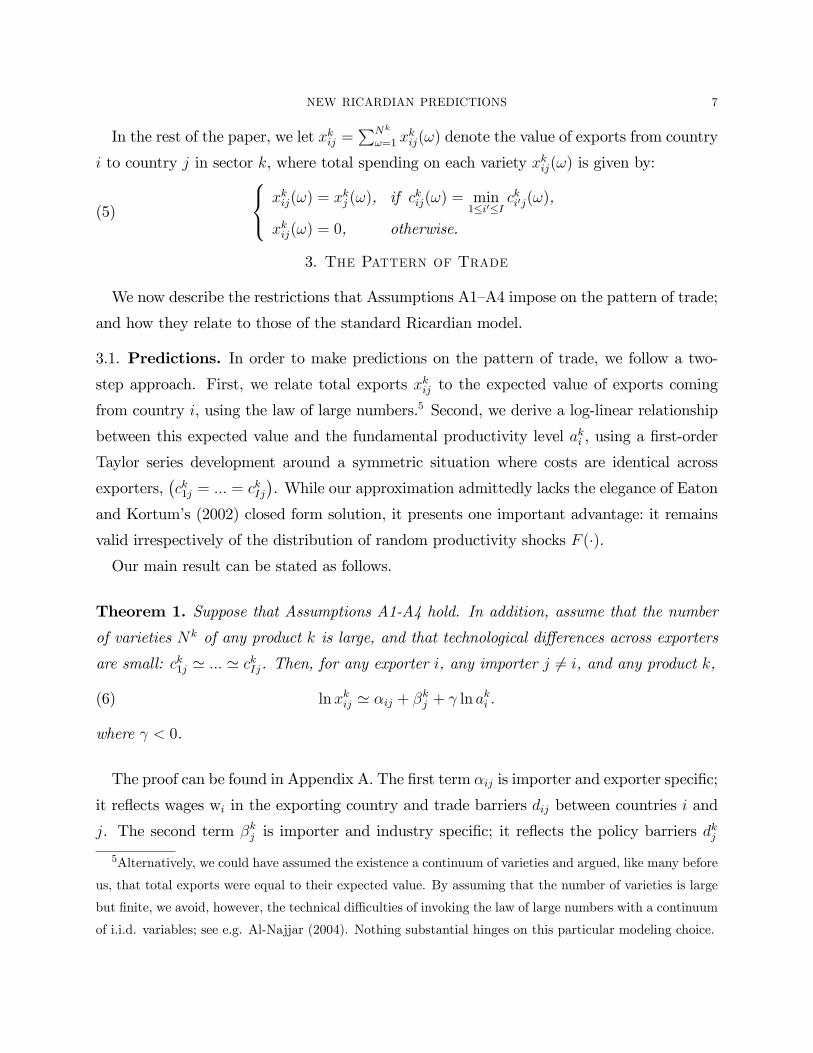
In the rest of the paper, we let xkij =PNk
!=1 xkij(!) denote the value of exports from country
i to country j in sector k, where total spending on each variety xkij(!) is given by:
(5)
8<: xkij(!) = xkj (!), if ckij(!) = min
1�i0�Icki0j(!),
xkij(!) = 0, otherwise.
3. The Pattern of Trade
We now describe the restrictions that Assumptions A1�A4 impose on the pattern of trade;
and how they relate to those of the standard Ricardian model.
3.1. Predictions. In order to make predictions on the pattern of trade, we follow a two-
step approach. First, we relate total exports xkij to the expected value of exports coming
from country i, using the law of large numbers.5 Second, we derive a log-linear relationship
between this expected value and the fundamental productivity level aki , using a �rst-order
Taylor series development around a symmetric situation where costs are identical across
exporters,�ck1j = ::: = c
kIj
�. While our approximation admittedly lacks the elegance of Eaton
and Kortum�s (2002) closed form solution, it presents one important advantage: it remains
valid irrespectively of the distribution of random productivity shocks F (�).Our main result can be stated as follows.
Theorem 1. Suppose that Assumptions A1-A4 hold. In addition, assume that the number
of varieties Nk of any product k is large, and that technological di¤erences across exporters
are small: ck1j ' ::: ' ckIj. Then, for any exporter i, any importer j 6= i, and any product k,
(6) lnxkij ' �ij + �kj + ln aki :
where < 0.
The proof can be found in Appendix A. The �rst term �ij is importer and exporter speci�c;
it re�ects wages wi in the exporting country and trade barriers dij between countries i and
j. The second term �kj is importer and industry speci�c; it re�ects the policy barriers dkj
5Alternatively, we could have assumed the existence a continuum of varieties and argued, like many before
us, that total exports were equal to their expected value. By assuming that the number of varieties is large
but �nite, we avoid, however, the technical di¢ culties of invoking the law of large numbers with a continuum
of i.i.d. variables; see e.g. Al-Najjar (2004). Nothing substantial hinges on this particular modeling choice.
8 COSTINOT AND KOMUNJER
imposed by country j on product k and demand di¤erences ekj across countries and industries.
The main insight of Theorem 1 comes from the third term ln aki . Since < 0, lnxkij should
be decreasing in ln aki : ceteris paribus, countries should export less in sectors where their
�rms are, on average, less e¢ cient.
The predictive power of our theory crucially relies on the fact that is constant across
countries and industries. To understand this result, it is convenient to think about total
exports in terms of their extensive and intensive margins, that is how many and how much of
each variety are being exported, respectively. The unique distribution of random productivity
shocks F (�) makes sure that marginal changes in the costs of production ckij have the sameimpact on the extensive margin across countries and industries. Similarly, the constant
elasticity of substitution � guarantees that they have the same impact on the intensive
margin. This is the basic idea behind Theorem 1. The other assumptions simply allow us to
identify the e¤ect of labor productivity by bundling the impact of changes in wages, demand,
and transport costs into �xed e¤ects.
It is worth emphasizing that Theorem 1 cannot be used for comparative static analysis. If
the fundamental productivity level goes up in a given country and industry, this will a¤ect
wages and, in turn, exports in other countries and industries through general equilibrium
e¤ects. In other words, changes in aki also lead to changes in the country and industry
�xed e¤ects, �ij and �kj . By contrast, Theorem 1 can be used to analyze the cross-sectional
variations of bilateral exports, as we shall further explore in Section 4.
Though the assumptions of Theorem 1 may seem unreasonably strong� in practice, tech-
nological di¤erences across all exporters are unlikely to be small� its predictions hold more
generally. Suppose that, for each product and each importing country, exporters can be
separated into two groups: small exporters, whose costs are very large (formally, close to
in�nity), and large exporters, whose costs of production are small and of similar magnitude.
Then, small exporters export with probability close to zero and the results of Theorem 1
still apply to the group of large exporters.6
If we impose more structure on the distribution of random productivity shocks, we can
further weaken the assumptions of Theorem 1. Suppose that the distribution F (�) of uki (!)
6In other words, our theory does not require Gambia and Japan to have similar costs of producing and
delivering cars in the United States. It simply requires that Japan and Germany do.
NEW RICARDIAN PREDICTIONS 9
is Gumbel as in Eaton and Kortum (2002). Then, it can be shown that the property in
Equation (6) holds exactly for any�ck1j; :::; c
kIj
�. In other words, if Eaton and Kortum�s (2002)
distributional assumption is satis�ed, then our local results become global; they extend to
environments where technological di¤erences across all countries are large.
If F (�) is Gumbel, one can further show that �ij, �kj , and do not depend on the elasticityof substitution �. In this case, the predictions of Theorem 1 still hold if we relax Assumption
A4(i), so that the elasticity of substitution may vary across countries and industries, � � �kj .This derives from a key property of the Gumbel distribution: conditional on exporting a
given variety to country j, the expected value of exports has to be identical across countries.
Hence, transport costs, wages and fundamental productivity levels only a¤ect the extensive
margin, not the intensive margin. This convenient property, however, does not generalize to
other standard distributions; see Appendix C.
In order to prepare the comparison between our results and those of the standard Ricardian
model, we conclude this section by o¤ering a Corollary to Theorem 1. Consider an arbitrary
pair of exporters i1 and i2, an importer j 6= i1; i2 and an arbitrary pair of goods k1 and k2.Taking the di¤erences-in-di¤erences in Equation (6) we get that (lnxk1i1j� lnx
k2i1j)� (lnxk1i2j�
lnxk2i2j) ' ��ln ak1i1 � ln a
k2i1
���ln ak1i2 � ln a
k2i2
��, for Nk1 and Nk2 large enough. Since < 0,
we then obtain that
(7)ak1i1ak1i2
>ak2i1ak2i2
)xk1i1j
xk1i2j<xk2i1j
xk2i2j:
Still considering the pair of exporters i1 and i2 and generalizing the above reasoning to all
K products, we derive the following Corollary:
Corollary 2. Suppose that the assumptions of Theorem 1 hold. Then, the ranking of relative
unit labor requirements determines the ranking of relative exports:�a1i1a1i2
> :::: >aki1aki2
> ::: >aKi1aKi2
�)(x1i1jx1i2j
< :::: <xki1jxki2j
< ::: <xKi1jxKi2j
):
3.2. Relation to the standard Ricardian model. Note that we can always index the K
products so that:
(8)a1i1a1i2
> :::: >aki1aki2
> ::: >aKi1aKi2:
10 COSTINOT AND KOMUNJER
Ranking (8) is at the heart of the standard Ricardian model; see e.g. Dornbusch, Fischer,
and Samuelson (1977). When there are no random productivity shocks, Ranking (8) merely
states that country i1 has a comparative advantage in (all varieties of) the high k products.
If there only are two countries, the pattern of trade follows: i1 produces and exports the
high k products, while i2 produces and exports the low k products. If there are more than
two countries, however, the pattern of pairwise comparative advantage no longer determines
the pattern of trade. In this case, the standard Ricardian model loses most of its intuitive
content; see e.g. Jones (1961) and Wilson (1980).
When there are stochastic productivity di¤erences within each industry, Assumption A1
and Ranking (8) further imply:
(9)a1i1(!)
a1i2(!)� :::: �
aki1(!)
aki2(!)� ::: �
aKi1 (!)
aKi2 (!);
where � denotes the �rst-order stochastic dominance order among distributions.7 In other
words, Ranking (9) is just a stochastic� hence weaker� version of the ordering of labor
requirements aki , which is at the heart of the Ricardian theory. Like its deterministic coun-
terpart in (8), Ranking (9) captures the idea that country i1 is relatively better at producing
the high k products. But whatever k is, country i2 may still have lower labor requirements
on some of its varieties.
According to Corollary 2, Ranking (9) does not imply that country i1 should only produce
and export the high k products, but instead that it should produce and export relatively more
of these products. This is true irrespective of the number of countries in the economy. Unlike
the standard Ricardian model, our stochastic theory of comparative advantage generates a
clear and intuitive correspondence between labor productivity and exports. In our model,
the pattern of comparative advantage for any pair of exporters fully determines their relative
export performance across industries.
7To see this, note that for any A 2 R+ we have Pr�aki1(!)=a
ki2(!) � A
= Prfuki1(!) � u
ki2(!) � lnA �
ln aki1+ln aki2g . Since for any k < k0, uki1(!)�u
ki2(!) and uk
0
i1(!)�uk0i2 (!) are drawn from the same distribution
by A1, Ranking (8) implies:
Pr
(aki1(!)
aki2(!)� A
)< Pr
(ak
0
i1(!)
ak0i2(!)
� A),aki1(!)
aki2(!)�ak
0
i1(!)
ak0i2(!)
NEW RICARDIAN PREDICTIONS 11
This may seem paradoxical. As we have just mentioned, Ranking (9) is a weaker version
of the ordering at the heart of the standard theory. If so, how does our stochastic theory
lead to �ner predictions? The answer is simple: it does not. While the standard Ricardian
model is concerned with trade �ows in each variety of each product, we only are concerned
with the total trade �ows in each product. Unlike the standard model, we recognize that
random shocks� whose origins remain outside the scope of our model� may a¤ect the costs
of production of any variety. Yet, by assuming that these shocks are identically distributed
across a large number of varieties, we manage to generate sharp predictions at the industry
level.
4. Empirical Evidence
We now investigate whether the predictions of Theorem 1 are consistent with the data.
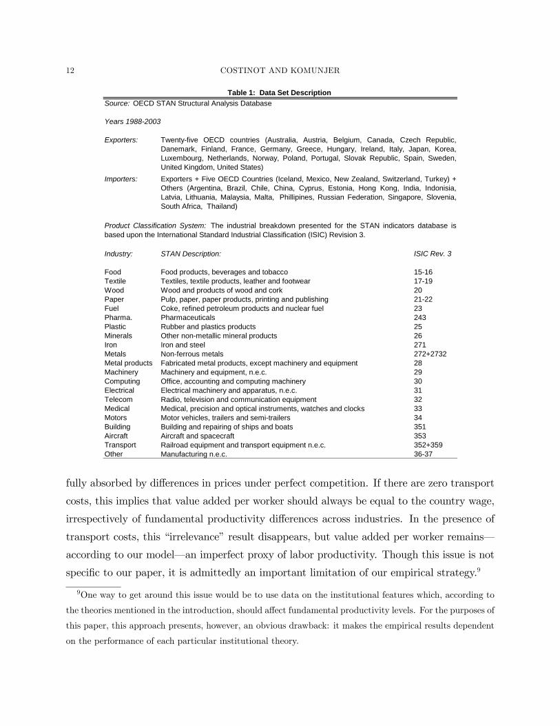
4.1. Data description. We use yearly data from the OECD Structural Analysis (STAN)
Databases from 1988 to 2003. Our sample includes 25 exporters, all OECD countries, and
49 importers, both OECD and non-OECD countries. It covers 21 manufacturing sectors
aggregated (roughly) at the 2-digit ISIC rev 3 level. To the best of our knowledge, it
corresponds to the largest data set available with both bilateral trade data and comparable
labor productivity data. See Table 1 for details.
The value of exports xkij by exporting country i, importing country j, and industry k
is directly available (in thousands of US dollars, at current prices) in the STAN Bilateral
Trade Database. The unit labor requirement aki in country i and industry k is measured
as total employment divided by value added (in millions or billions of national currency, at
current prices), which can both be found in the STAN Industry Database.8 Appendix D
o¤ers additional details on the variations of value added per worker in our sample.
Despite the virtue of tradition, there are concerns with this measure of labor productivity.
As Bernard, Eaton, Jensen, and Kortum (2003) point out, di¤erences in productivity are
8Any di¤erence in units of account across countries shall be treated as an exporter �xed e¤ect in our
regression (10). Hence, we do not need to convert our measures of aki into a common currency. Similarly, we
do not correct for the number of hours worked per person and per year, which only is available for a very
small fraction of our sample. But it should be clear that cross-country di¤erences in hours worked will also
be captured by our exporter �xed e¤ect.
12 COSTINOT AND KOMUNJER
Years 19882003
Exporters:
Importers:
Industry: ISIC Rev. 3
Food 1516Textile 1719Wood 20Paper 2122Fuel 23Pharma. 243Plastic 25Minerals 26Iron 271Metals 272+2732Metal products 28Machinery 29Computing 30Electrical 31Telecom 32Medical 33Motors 34Building 351Aircraft 353Transport 352+359Other 3637
Aircraft and spacecraftRailroad equipment and transport equipment n.e.c.Manufacturing n.e.c.
Source: OECD STAN Structural Analysis Database
Product Classification System: The industrial breakdown presented for the STAN indicators database isbased upon the International Standard Industrial Classification (ISIC) Revision 3.
Radio, television and communication equipmentMedical, precision and optical instruments, watches and clocksMotor vehicles, trailers and semitrailersBuilding and repairing of ships and boats
Other nonmetallic mineral productsIron and steelNonferrous metals
Electrical machinery and apparatus, n.e.c.Office, accounting and computing machineryMachinery and equipment, n.e.c.Fabricated metal products, except machinery and equipment
Table 1: Data Set Description
STAN Description:
Twentyfive OECD countries (Australia, Austria, Belgium, Canada, Czech Republic,Danemark, Finland, France, Germany, Greece, Hungary, Ireland, Italy, Japan, Korea,Luxembourg, Netherlands, Norway, Poland, Portugal, Slovak Republic, Spain, Sweden,United Kingdom, United States)
Textiles, textile products, leather and footwearFood products, beverages and tobacco
PharmaceuticalsRubber and plastics products
Exporters + Five OECD Countries (Iceland, Mexico, New Zealand, Switzerland, Turkey) +Others (Argentina, Brazil, Chile, China, Cyprus, Estonia, Hong Kong, India, Indonisia,Latvia, Lithuania, Malaysia, Malta, Phillipines, Russian Federation, Singapore, Slovenia,South Africa, Thailand)
Wood and products of wood and corkPulp, paper, paper products, printing and publishingCoke, refined petroleum products and nuclear fuel
fully absorbed by di¤erences in prices under perfect competition. If there are zero transport
costs, this implies that value added per worker should always be equal to the country wage,
irrespectively of fundamental productivity di¤erences across industries. In the presence of
transport costs, this �irrelevance�result disappears, but value added per worker remains�
according to our model� an imperfect proxy of labor productivity. Though this issue is not
speci�c to our paper, it is admittedly an important limitation of our empirical strategy.9
9One way to get around this issue would be to use data on the institutional features which, according to
the theories mentioned in the introduction, should a¤ect fundamental productivity levels. For the purposes of
this paper, this approach presents, however, an obvious drawback: it makes the empirical results dependent
on the performance of each particular institutional theory.
NEW RICARDIAN PREDICTIONS 13
4.2. Speci�cation. The main qualitative insight of our model is that:
(@ lnxkij)=�@ ln aki
�= < 0
In other words, the elasticity of exports with respect to the average unit labor requirement
should be negative and constant across importers, exporters, and industries. Accordingly,
we shall consider a linear regression model of the form
(10) lnxkij = �ij + �kj + ln a
ki + "
kij;
where �ij and �kj are treated as importer�exporter and importer�industry �xed e¤ects, re-
spectively, and "kij is an error term.
There are (at least) two possible interpretations of the error term "kij. First, we can think
of "kij as a measurement error in trade �ows. This is the standard approach in the gravity
literature; see e.g. Anderson and Wincoop (2003). Alternatively, we can think of "kij as
representing the impact of unobserved trade barriers, not accounted for in Assumption A2.
Indeed, we can generalize A2 as ln dkij = ln dij + ln dkj + e"kij. Then, setting "kij = e"kij� and
using the expressions of �ij and �kj provided in the proof of Theorem 1� immediately leads
to Equation (10). This is the approach followed by Eaton and Kortum (2002) and Helpman,
Melitz, and Rubinstein (2005). Under either interpretation, we shall assume that "kij is
independent across countries i and j as well as across industries k; that "kij is heteroskedastic
conditional on i, j and k; and that "kij is uncorrelated with ln aki .
Note that our orthogonality condition rules out situations where country j tends to dis-
criminate more against country i in sectors where i is more productive. Were these situations
prevalent in practice, due to endogenous trade protection, our OLS estimates of would be
biased (upward) towards zero.10 Similarly, our orthogonality condition rules out any poten-
tial errors in the measurement of labor productivity at the industry level, which obviously
10Formally, suppose that trade barriers, dkij , and exports, xkij , are simultaneously determined according
to 8<: ln dkij = ln dij + ln dkj + � lnx
kij
lnxkij = �̂ij + �̂k
j + ln aki + ln d
kij
where � > 0 captures the fact that higher levels of import penetration lead to higher levels of protection.
The previous system can be rearranged as8<: ln dkij = (1� � )�1[ln dij + ln dkj + ��̂ij + ��̂k
j + � ln aki ]
lnxkij = �ij + �kj + ln a
ki + "
kij
14 COSTINOT AND KOMUNJER
Variable 2003 2002 2001 2000 1999 1998 1997 1996ln a 0.78 0.67 0.91 0.80 0.71 0.89 0.95 0.73
(10.31)*** (12.74)*** (16.47)*** (15.91)*** (12.87)*** (13.72)*** (14.16)*** (10.69)***ExporterImporter FE Yes Yes Yes Yes Yes Yes Yes YesIndustryImporter FE Yes Yes Yes Yes Yes Yes Yes YesObservations 8778 15051 18167 18597 18805 18187 18233 17780R2 0.805 0.794 0.793 0.787 0.792 0.792 0.789 0.785
Variable 1995 1994 1993 1992 1991 1990 1989 1988ln a 0.79 0.75 0.53 0.50 0.42 0.37 0.39 0.08
(12.22)*** (9.79)*** (7.74)*** (7.03)*** (5.60)*** (5.05)*** (5.77)*** (1.06)ExporterImporter FE Yes Yes Yes Yes Yes Yes Yes YesIndustryImporter FE Yes Yes Yes Yes Yes Yes Yes YesObservations 17423 14245 13489 12755 11827 11655 11606 10672R2 0.7849 0.7877 0.7936 0.7936 0.783 0.780 0.779 0.776Note: Values of tstatistics in parentheses are calculated from heteroskedasticityconsistent (White) standard errors* Significant at 10% confidence level** Significant at 5% confidence level*** Significant at 1% confidence level
Table 2: YearbyYear OLS Regressions(Dependent Variable: lnx)
is a very strong assumption. The presence of measurement errors in the data should further
bias our OLS estimates of (upward) towards zero.
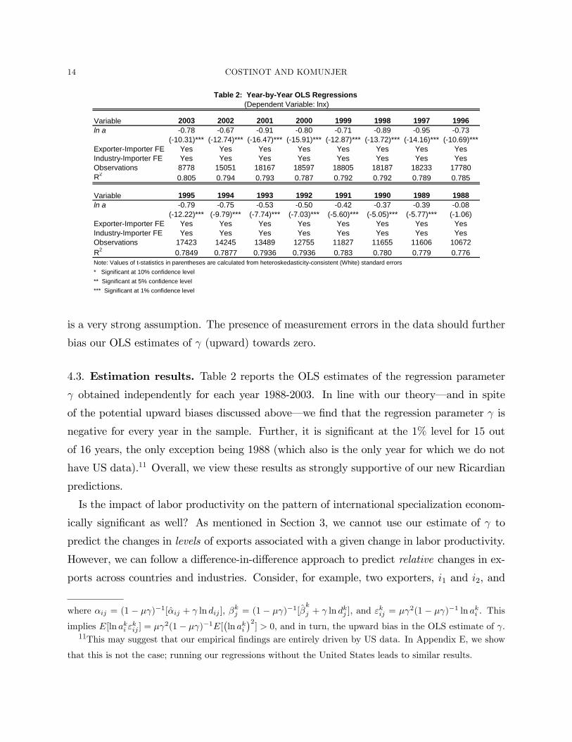
4.3. Estimation results. Table 2 reports the OLS estimates of the regression parameter
obtained independently for each year 1988-2003. In line with our theory� and in spite
of the potential upward biases discussed above� we �nd that the regression parameter is
negative for every year in the sample. Further, it is signi�cant at the 1% level for 15 out
of 16 years, the only exception being 1988 (which also is the only year for which we do not
have US data).11 Overall, we view these results as strongly supportive of our new Ricardian
predictions.
Is the impact of labor productivity on the pattern of international specialization econom-
ically signi�cant as well? As mentioned in Section 3, we cannot use our estimate of to
predict the changes in levels of exports associated with a given change in labor productivity.
However, we can follow a di¤erence-in-di¤erence approach to predict relative changes in ex-
ports across countries and industries. Consider, for example, two exporters, i1 and i2, and
where �ij = (1 � � )�1[�̂ij + ln dij ], �kj = (1 � � )�1[�̂k
j + ln dkj ], and "
kij = �
2(1 � � )�1 ln aki . Thisimplies E[ln aki "
kij ] = �
2(1� � )�1E[�ln aki
�2] > 0, and in turn, the upward bias in the OLS estimate of .
11This may suggest that our empirical �ndings are entirely driven by US data. In Appendix E, we show
that this is not the case; running our regressions without the United States leads to similar results.
NEW RICARDIAN PREDICTIONS 15
two industries, k1 and k2, in 2003. If ak1i1decreases by 10%, then our prediction is that:�
� lnxk1i1j �� lnxk2i1j
���� lnxk1i2j �� lnx
k2i2j
�= b 2003� ln ak1i1 ' 7:8%:
This is consistent with a scenario where country i1�s exports of good k1 go up by 5% and
(because of the associated wage increase in country i1) those of k2 go down by 2:8%, while
they remain unchanged in both sectors in country i2.
To help understand the size of the e¤ects reported in Table 2, we can also use the standard
deviations of ln aki and lnxkij in 2003, 1:30 and 2:91, respectively. Our estimates suggest that,
ceteris paribus, a one standard deviation decrease in ln aki should increase the dependent
variable by 0:35 standard deviations.
4.4. Relation to the previous empirical literature. As mentioned in the introduction,
previous Ricardian �tests�were remarkably successful. In light of this evidence, it is perhaps
not too surprising to uncover, as we just did, a positive association between productivity
and trade �ows in the data.12
Nevertheless, we believe that the tight connection between the theory and the empirical
analysis that our paper o¤ers is a signi�cant step beyond the existing literature. First, we
do not have to rely on ad-hoc measures of export performance such as total exports towards
the rest of the world (MacDougall (1951) and Stern (1962)); total exports to third markets
(Balassa (1963)); or bilateral net exports (Golub and Hsieh (2000)). The theory tells us ex-
actly what the dependent variable in the cross-industry regressions ought to be: ln(exports),
disaggregated by exporting and importing countries. Second, the careful introduction of
country and industry �xed e¤ects allows us to move away from the bilateral comparisons
inspired by the two-country model, and in turn, to take advantage of a much richer data set.
Third, our clear theoretical foundations make it possible to discuss the economic origins of
the error terms� measurement errors in trade �ows or unobserved trade barriers� and as a
result, the plausibility of our orthogonality conditions.
12In terms of magnitude, our estimates lie between those of the early Ricardian �tests�� MacDougall
(1951), Stern (1962), and Balassa (1963)� and the more recent �ndings of Golub and Hsieh (2000). Using
US and UK data, MacDougall (1951), Stern (1962), and Balassa (1963) �nd elasticities of exports with
respect to average unit labor requirements around �1:6. By contrast, the highest elasticity estimated byGolub and Hsieh (2000) is equal to �0:37; see Table 2 p228.
16 COSTINOT AND KOMUNJER
Of course, one might argue that the model developed in this paper� Assumptions A1-A4�
is not the only way to bring the Ricardian model to the data. For example, we could also
obtain Equation (10) by directly imposing Armington�s preferences. While this is certainly
true, the attractiveness of our approach lies in the weakness of the assumptions under which
Equation (10) is derived. As long as there are stochastic productivity di¤erences within
each industry, our analysis demonstrates that many of the assumptions usually invoked to
rationalize cross-industry regressions� either on preferences or on transport costs� can be
relaxed. Put simply, our paper may not o¤er researchers brand new regressions to run, but
we hope it can make them more comfortable running them.
In particular, we think that our theoretical approach may be fruitfully applied to more
general environments, where labor is not the only factor of production. The basic idea,
already suggested by Bhagwati (1964), is to reinterpret di¤erences in aki as di¤erences in
total factor productivity. With multiple factors of production, the volume of exports would
be a function of both technological di¤erences, captured by aki , and di¤erences in relative
factor prices.13 The rest of our analysis would remain unchanged.
5. Concluding Remarks
The Ricardian model has long been perceived has a useful pedagogical tool with, ulti-
mately, little empirical content. Over the last twenty years, the Heckscher-Ohlin model,
which emphasizes the role of cross-country di¤erences in factor endowments, has generated
a considerable amount of empirical work ; see e.g. Bowen, Leamer, and Sveikauskas (1987),
Tre�er (1993), Tre�er (1995), Davis and Weinstein (2001), and Schott (2004). The Ricardian
model, which emphasizes productivity di¤erences, almost none.
The main reason behind this lack of popularity is not the existence of strong beliefs
regarding the relative importance of factor endowments and technological considerations.
Previous empirical work on the Heckscher-Ohlin model unambiguously shows that technology
matters. It derives instead from the obvious mismatch between the real world and the
extreme predictions (and assumptions) of the standard Ricardian model. In the words of
Leamer and Levinsohn (1995), �[it] is just too simple.�
13Costinot�s (2005) chapter 3 and Chor (2006) incorporate multiple factors of production into the Eaton
and Kortum�s (2002) model along these lines.
NEW RICARDIAN PREDICTIONS 17
Although the de�ciencies of the Ricardian model have not lead to the disappearance of
technological considerations from the empirical literature, they have had a strong in�uence on
how the relationship between technology and trade has been studied. In the Heckscher-Ohlin-
Vanek literature� with or without technological di¤erences� the factor content of trade re-
mains the main variable of interest. Building on the seminal work of Eaton and Kortum
(2002), our paper develops a �robust� theoretical framework that puts back productivity
di¤erences at the forefront of the analysis.
References
Acemoglu, D., P. Antras, and E. Helpman (2007): �Contracts and Technology Adop-
tion,� forthcoming American Economic Review.
Al-Najjar, N. (2004): �Aggregation and the Law of Large Numbers in Large Economies,�
Games and Economic Behavior, pp. 1�35.
Anderson, J. A., and E. V. Wincoop (2003): �Gravity with Gravitas: A Solution to
the Border Puzzle,�The American Economic Review, pp. 170�192.
Antras, P., and E. Helpman (2004): �Global Sourcing,�Journal of Political Economy,
pp. 552�580.
Balassa, B. (1963): �An Empirical Demonstration of Comparative Cost Theory,�Review
of Economics and Statistics, pp. 231�238.
Bernard, A. B., J. Eaton, J. B. Jensen, and S. Kortum (2003): �Plants and Pro-
ductivity in International Trade,�The American Economic Review, pp. 1268�1290.
Bernard, A. B., S. J. Redding, and P. K. Schott (2006): �Comparative Advantage
and Heterogeneous Firms,�(forthcoming) The Review of Economic Studies.
Bhagwati, J. (1964): �The Pure Theory of International Trade: A Survey,�The Economic
Journal, pp. 1�84.
Billingsley, P. (1995): Probability and Measure. John Wiley & Sons, Inc.
Bowen, H. P., E. E. Leamer, and L. Sveikauskas (1987): �Multicountry, Multifactor
Tests of the Factor Abundance Theory,�The American Economic Review, pp. 791�809.
Chaney, T. (2007): �Distorted Gravity: The Intensive and Extensive Margins of Interna-
tional Trade,�mimeo University of Chicago.
18 COSTINOT AND KOMUNJER
Chor, D. (2006): �Unpacking Sources of Comparative Advantage: A Quantitative Ap-
proach,�mimeo Harvard University.
Costinot, A. (2005): �Three Essays on Institutions and Trade,� Ph.D. Dissertation,
Princeton University.
(2006): �On the Origins of Comparative Advantage,�mimeo University of Califor-
nia, San Diego.
Cuñat, A., and M. Melitz (2006): �Labor Market Flexibility and Comparative Advan-
tage,�mimeo Harvard University.
Davidson, J. (1994): Stochastic Limit Theory. Oxford University Press, Oxford.
Davis, D. R., and D. E. Weinstein (2001): �An Account of Global Factor Trade,�The
American Economic Review, pp. 1423�1453.
Deardorff, A. V. (1980): �The General Validity of the Law of Comparative Advantage,�
Journal of Political Economy, pp. 941�957.
(2005): �How Robust is Comparative Advantage,�mimeo University of Michigan.
Dornbusch, R., S. Fischer, and P. Samuelson (1977): �Comparative Advantage,
Trade, and Payments in a Ricardian Model with a Continuum of Goods,�American Eco-
nomic Review, 67, 823�839.
Eaton, J., and S. Kortum (2002): �Technology, Geography, and Trade,�Econometrica,
70, 1741�1779.
Ghironi, F., and M. Melitz (2005): �International Trade and Macroeconomic Dynamics
with Heterogeneous Firms,�Quarterly Journal of Economics, pp. 865�915.
Golub, S. S., and C.-T. Hsieh (2000): �Classical Ricardian Theory of Comparative
Advantage Revisited,�Review of International Economics, pp. 221�234.
Harrigan, J. (1997): �Technology, Factor Supplies, and International Specialization: Es-
timating the Neo-Classical Model,�The American Economic Review, pp. 475�494.
Helpman, E., and P. R. Krugman (1985): Market Structure and Foreign Trade. MIT
Press.
Helpman, E., M. Melitz, and Y. Rubinstein (2005): �Trading Partners and Trading
Volumes,�mimeo Harvard University.
Helpman, E., M. Melitz, and S. Yeaple (2004): �Export versus FDI with Heteroge-
neous Firms,�The American Economic Review, pp. 300�316.
NEW RICARDIAN PREDICTIONS 19
Jones, R. W. (1961): �Comparative Advantage and the Theory of Tari¤s: AMulti-Country,
Multi-Commodity Model,�The Review of Economic Studies, 28(3), 161�175.
Leamer, E., and J. Levinsohn (1995): �International Trade Theory: The Evidence,�
in Handbook of International Economics, ed. by G. Grossman, and K. Rogo¤, vol. 3, pp.
1139�1194. Elsevier Science, New York.
Levchenko, A. (2007): �Institutional Quality and International Trade,� forthcoming Re-
view of Economic Studies.
MacDougall, G. (1951): �British and American Exports: A Study Suggested by the
Theory of Comparative Costs, Part,�Economic Journal, pp. 697�724.
Matsuyama, K. (2005): �Credit Market Imperfections and Patterns of International Trade
and Capital Flows,�Journal of the European Economic Association, pp. 714�723.
Melitz, M. (2003): �The Impact of Trade on Intra-Industry Reallocations and Aggregate
Inudstry Productivity,�Econometrica, pp. 1695�1725.
Morrow, P. (2006): �East is East and West is West: A Ricardian-Heckscher-Ohlin Model
of Comparative Advantage,�mimeo Michigan University.
Nunn, N. (2007): �Relationship Speci�city, Incomplete Contracts and the Pattern of
Trade,� forthcoming Quarterly Journal of Economics.
Petri, P. A. (1980): �A Ricardian Model of Market Sharing,� Journal of International
Economics, pp. 201�211.
Romalis, J. (2004): �Factor Proportions and the Structure of Commodity Trade,� The
American Economic Review, pp. 67�97.
Schott, P. (2004): �Across-Product versus Within-Product Specialization in International
Trade,�Quarterly Journal of Economics, pp. 647�678.
Stern, R. M. (1962): �British and American Productivity and Comparative Costs in
International Trade,�Oxford Economic Papers, pp. 275�303.
Trefler, D. (1993): �International Factor Price Di¤erences: Leontief was Right!,�Journal
of Political Economy, pp. 961�987.
(1995): �The Case of the Missing Trade and Other Mysteries,� The American
Economic Review, pp. 1029�1046.
Vogel, J. (2007): �Institutions and Moral Hazard in Open Economies,�forthcoming Jour-
nal of International Economics.

20 COSTINOT AND KOMUNJER
Wilson, C. A. (1980): �On the General Structure of Ricardian Models with a Continuum
of Goods: Applications to Growth, Tari¤ Theory, and Technical Change,�Econometrica,
pp. 1675�1702.
NEW RICARDIAN PREDICTIONS 21
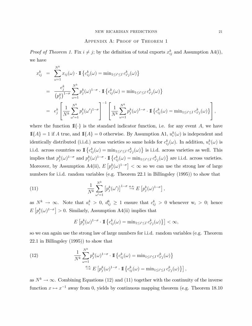
Appendix A: Proof of Theorem 1
Proof of Theorem 1. Fix i 6= j; by the de�nition of total exports xkij and Assumption A4(i),we have
xkij =
NkX!=1
xij(!) � 1I�ckij(!) = min1�i0�I c
ki0j(!)
=
ekj�pkj�1�� NkX
!=1
pkj (!)1�� � 1I
�ckij(!) = min1�i0�I c
ki0j(!)
= ekj
24 1
Nk
NkX!0=1
pkj (!0)1��
35�1 24 1
Nk
NkX!=1
pkj (!)1�� � 1I
�ckij(!) = min1�i0�I c
ki0j(!)
35 ;where the function 1If�g is the standard indicator function, i.e. for any event A, we have1IfAg = 1 if A true, and 1IfAg = 0 otherwise. By Assumption A1, uki (!) is independent andidentically distributed (i.i.d.) across varieties so same holds for ckij(!). In addition, u
ki (!) is
i.i.d. across countries so 1I�ckij(!) = min1�i0�I c
ki0j(!)
is i.i.d. across varieties as well. This
implies that pkj (!)1�� and pkj (!)
1�� � 1I�ckij(!) = min1�i0�I c
ki0j(!)
are i.i.d. across varieties.
Moreover, by Assumption A4(ii), E�pkj (!)
1��� < 1 so we can use the strong law of large
numbers for i.i.d. random variables (e.g. Theorem 22.1 in Billingsley (1995)) to show that
(11)1
Nk
NkX!0=1
�pkj (!
0)�1�� a:s:! E
�pkj (!)
1��� ;as Nk ! 1. Note that aki > 0, dkij � 1 ensure that ckij > 0 whenever wi > 0; hence
E�pkj (!)
1��� > 0. Similarly, Assumption A4(ii) implies thatE�pkj (!)
1�� � 1I�ckij(!) = min1�i0�I c
ki0j(!)
�<1;
so we can again use the strong law of large numbers for i.i.d. random variables (e.g. Theorem
22.1 in Billingsley (1995)) to show that
1
Nk
NkX!=1
pkj (!)1�� � 1I
�ckij(!) = min1�i0�I c
ki0j(!)
(12)
a:s:! E�pkj (!)
1�� � 1I�ckij(!) = min1�i0�I c
ki0j(!)
�;
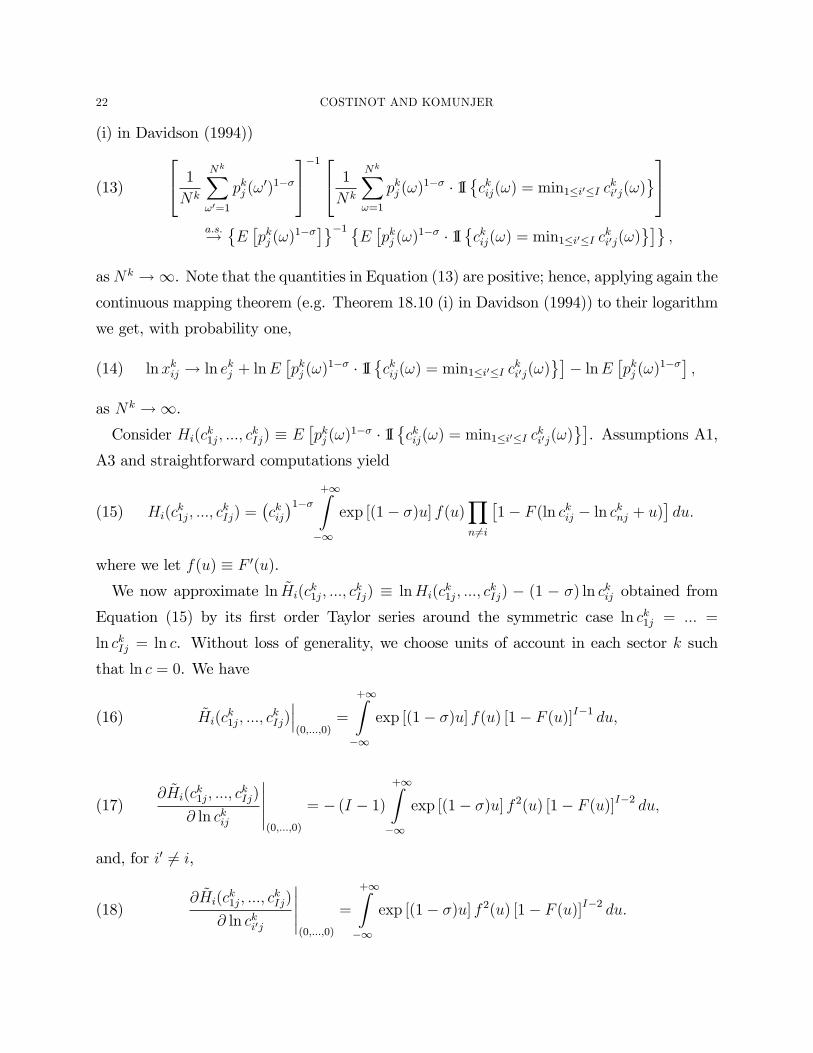
as Nk !1. Combining Equations (12) and (11) together with the continuity of the inversefunction x 7! x�1 away from 0, yields by continuous mapping theorem (e.g. Theorem 18.10
22 COSTINOT AND KOMUNJER
(i) in Davidson (1994))24 1
Nk
NkX!0=1
pkj (!0)1��
35�1 24 1
Nk
NkX!=1
pkj (!)1�� � 1I
�ckij(!) = min1�i0�I c
ki0j(!)
35(13)
a:s:!�E�pkj (!)
1����1 �E �pkj (!)1�� � 1I�ckij(!) = min1�i0�I cki0j(!)� ;asNk !1. Note that the quantities in Equation (13) are positive; hence, applying again thecontinuous mapping theorem (e.g. Theorem 18.10 (i) in Davidson (1994)) to their logarithm
we get, with probability one,
(14) lnxkij ! ln ekj + lnE�pkj (!)
1�� � 1I�ckij(!) = min1�i0�I c
ki0j(!)
�� lnE
�pkj (!)
1��� ;as Nk !1.Consider Hi(ck1j; :::; c
kIj) � E
�pkj (!)
1�� � 1I�ckij(!) = min1�i0�I c
ki0j(!)
�. Assumptions A1,
A3 and straightforward computations yield
(15) Hi(ck1j; :::; c
kIj) =
�ckij�1�� +1Z
�1
exp [(1� �)u] f(u)Yn6=i
�1� F (ln ckij � ln cknj + u)
�du:
where we let f(u) � F 0(u).We now approximate ln ~Hi(ck1j; :::; c
kIj) � lnHi(c
k1j; :::; c
kIj) � (1 � �) ln ckij obtained from
Equation (15) by its �rst order Taylor series around the symmetric case ln ck1j = ::: =
ln ckIj = ln c. Without loss of generality, we choose units of account in each sector k such
that ln c = 0. We have
(16) ~Hi(ck1j; :::; c
kIj)���(0;:::;0)
=
+1Z�1
exp [(1� �)u] f(u) [1� F (u)]I�1 du;
(17)@ ~Hi(c
k1j; :::; c
kIj)
@ ln ckij
�����(0;:::;0)
= � (I � 1)+1Z�1
exp [(1� �)u] f 2(u) [1� F (u)]I�2 du;
and, for i0 6= i,
(18)@ ~Hi(c
k1j; :::; c
kIj)
@ ln cki0j
�����(0;:::;0)
=
+1Z�1
exp [(1� �)u] f 2(u) [1� F (u)]I�2 du:
NEW RICARDIAN PREDICTIONS 23
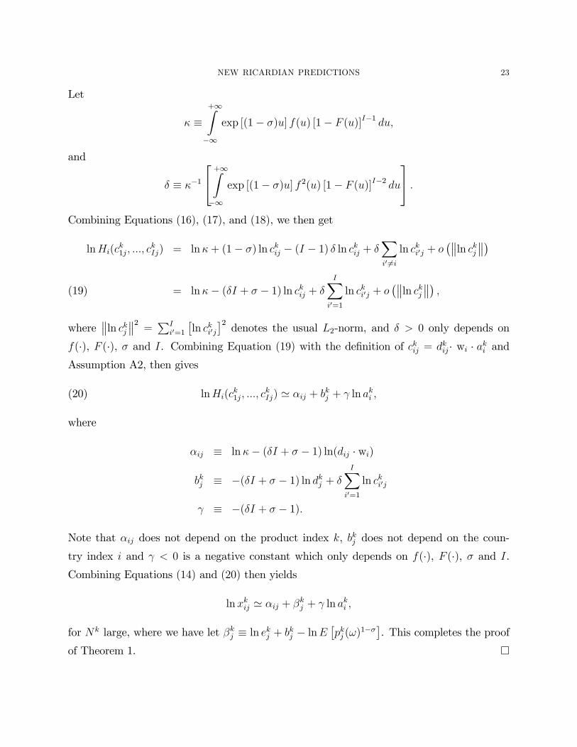
Let
� �+1Z�1
exp [(1� �)u] f(u) [1� F (u)]I�1 du;
and
� � ��124 +1Z�1
exp [(1� �)u] f 2(u) [1� F (u)]I�2 du
35 :Combining Equations (16), (17), and (18), we then get
lnHi(ck1j; :::; c
kIj) = ln�+ (1� �) ln ckij � (I � 1) � ln ckij + �
Xi0 6=i
ln cki0j + o� ln ckj �
= ln�� (�I + � � 1) ln ckij + �IX
i0=1
ln cki0j + o� ln ckj � ;(19)
where ln ckj 2 = PI
i0=1
�ln cki0j
�2denotes the usual L2-norm, and � > 0 only depends on
f(�), F (�), � and I. Combining Equation (19) with the de�nition of ckij = dkij� wi � aki andAssumption A2, then gives
(20) lnHi(ck1j; :::; c
kIj) ' �ij + bkj + ln aki ;
where
�ij � ln�� (�I + � � 1) ln(dij � wi)
bkj � �(�I + � � 1) ln dkj + �IX
i0=1
ln cki0j
� �(�I + � � 1):
Note that �ij does not depend on the product index k, bkj does not depend on the coun-
try index i and < 0 is a negative constant which only depends on f(�), F (�), � and I.Combining Equations (14) and (20) then yields
lnxkij ' �ij + �kj + ln aki ;
for Nk large, where we have let �kj � ln ekj + bkj � lnE�pkj (!)
1���. This completes the proofof Theorem 1. �
24 COSTINOT AND KOMUNJER
Appendix B: Bertrand Competition
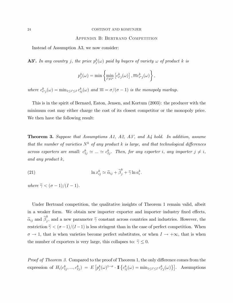
Instead of Assumption A3, we now consider:
A3�. In any country j, the price pkj (!) paid by buyers of variety ! of product k is
pkj (!) = min
�mini0 6=i�
�cki0j(!)
�;mcki�j(!)
�;
where cki�j(!) = min1�i0�I ckij(!) and m = �=(� � 1) is the monopoly markup.
This is in the spirit of Bernard, Eaton, Jensen, and Kortum (2003): the producer with the
minimum cost may either charge the cost of its closest competitor or the monopoly price.
We then have the following result:
Theorem 3. Suppose that Assumptions A1, A2, A3�, and A4 hold. In addition, assume
that the number of varieties Nk of any product k is large, and that technological di¤erences
across exporters are small: ck1j ' ::: ' ckIj. Then, for any exporter i, any importer j 6= i,
and any product k,
(21) lnxkij ' e�ij + e�kj + e ln aki :where e < (� � 1)=(I � 1).Under Bertrand competition, the qualitative insights of Theorem 1 remain valid, albeit
in a weaker form. We obtain new importer�exporter and importer�industry �xed e¤ects,e�ij and e�kj , and a new parameter e constant across countries and industries. However, therestriction e < (��1)=(I�1) is less stringent than in the case of perfect competition. When� ! 1, that is when varieties become perfect substitutes, or when I ! +1, that is whenthe number of exporters is very large, this collapses to: e � 0.Proof of Theorem 3. Compared to the proof of Theorem 1, the only di¤erence comes from the
expression of Hi(ck1j; :::; ckIj) = E
�pkj (!)
1�� � 1I�ckij(!) = min1�i0�I c
ki0j(!)
�. Assumptions
NEW RICARDIAN PREDICTIONS 25
A1, A3�and straightforward computations now yield
Hi(ck1j; :::; c
kIj) =
�ckij�1�� +1Z
�1
f(u1)du1
+1Zu1
[min (expu2;m expu1)]1�� �(22)
Xi0 6=i
( Yi00 6=i;i0
�1� F (ln ckij � ln cki00j + u2)
�f(ln ckij � ln cki0j + u2)
)du2:
where we let f(u) � F 0(u).As previously, we approximate ln ~Hi(ck1j; :::; c
kIj) � lnHi(ck1j; :::; ckIj)�(1��) ln ckij, obtained
from Equation (22), by its �rst order Taylor series around the symmetric case ln ck1j = ::: =
ln ckIj = 0. We have
~Hi(ck1j; :::; c
kIj)���(0;:::;0)
=
+1Z�1
f (u1) du1
+1Zu1
[min (expu2;m expu1)]1�� �
(I � 1) [1� F (u2)]I�2 f(u2)du2;(23)
@ ~Hi(ck1j; :::; c
kIj)
@ ln ckij
�����(0;:::;0)
= � (I � 1)+1Z�1
f (u1) du1
+1Zu1
[min (expu2;m expu1)]1�� �
n�f 0(u2) [1� F (u2)]I�2 + (I � 2) f 2 (u2) [1� F (u2)]I�3
odu2;(24)
and, for i0 6= i,
@Hi(ck1j; :::; c
kIj)
@ ln cki0j
�����(0;:::;0)
=
+1Z�1
f (u1) du1
+1Zu1
[min (expu2;m expu1)]1�� �
n�f 0(u2) [1� F (u2)]I�2 + (I � 2) f 2 (u2) [1� F (u2)]I�3
odu2:(25)
Let then
(26) � � (I � 1)+1Z�1
f (u1) du1
+1Zu1
[min (expu2;m expu1)]1�� [1� F (u2)]I�2 f(u2)du2;
26 COSTINOT AND KOMUNJER
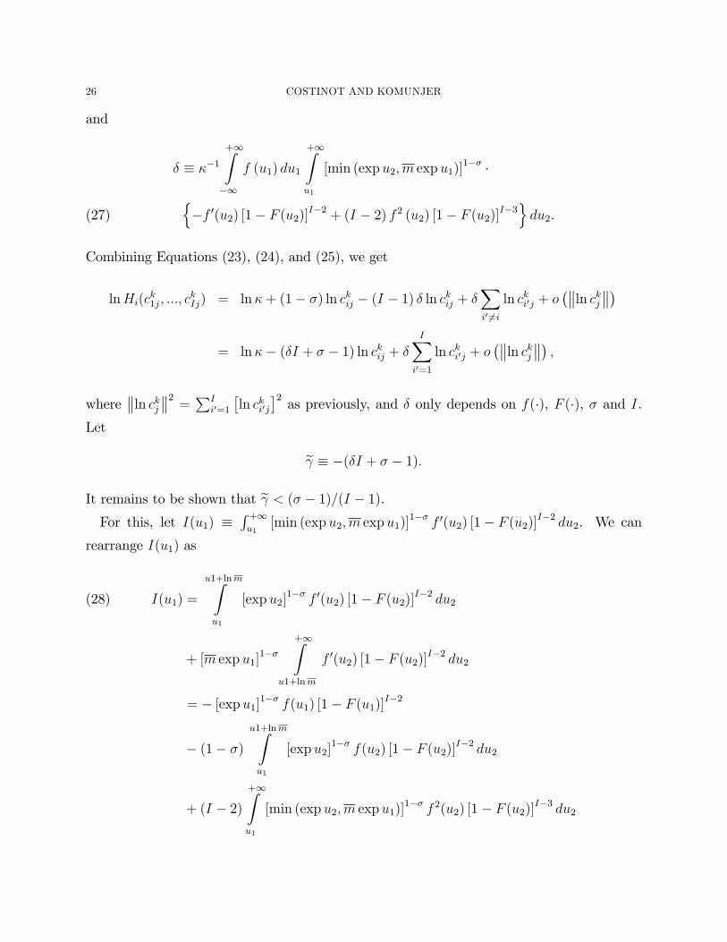
and
� � ��1+1Z�1
f (u1) du1
+1Zu1
[min (expu2;m expu1)]1�� �
n�f 0(u2) [1� F (u2)]I�2 + (I � 2) f 2 (u2) [1� F (u2)]I�3
odu2:(27)
Combining Equations (23), (24), and (25), we get
lnHi(ck1j; :::; c
kIj) = ln�+ (1� �) ln ckij � (I � 1) � ln ckij + �
Xi0 6=i
ln cki0j + o� ln ckj �
= ln�� (�I + � � 1) ln ckij + �IX
i0=1
ln cki0j + o� ln ckj � ;
where ln ckj 2 = PI
i0=1
�ln cki0j
�2as previously, and � only depends on f(�), F (�), � and I.
Let
e � �(�I + � � 1):It remains to be shown that e < (� � 1)=(I � 1).For this, let I(u1) �
R +1u1
[min (expu2;m expu1)]1�� f 0(u2) [1� F (u2)]I�2 du2. We can
rearrange I(u1) as
I(u1) =
u1+lnmZu1
[expu2]1�� f 0(u2) [1� F (u2)]I�2 du2(28)
+ [m expu1]1��
+1Zu1+lnm
f 0(u2) [1� F (u2)]I�2 du2
= � [expu1]1�� f(u1) [1� F (u1)]I�2
� (1� �)u1+lnmZu1
[expu2]1�� f(u2) [1� F (u2)]I�2 du2
+ (I � 2)+1Zu1
[min (expu2;m expu1)]1�� f 2(u2) [1� F (u2)]I�3 du2
NEW RICARDIAN PREDICTIONS 27
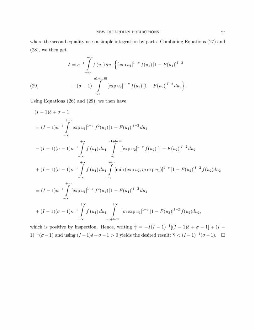
where the second equality uses a simple integration by parts. Combining Equations (27) and
(28), we then get
� = ��1+1Z�1
f (u1) du1
n[expu1]
1�� f(u1) [1� F (u1)]I�2
� (� � 1)u1+lnmZu1
[expu2]1�� f(u2) [1� F (u2)]I�2 du2
o:(29)
Using Equations (26) and (29), we then have
(I � 1)� + � � 1
= (I � 1)��1+1Z�1
[expu1]1�� f 2(u1) [1� F (u1)]I�2 du1
� (I � 1)(� � 1)��1+1Z�1
f (u1) du1
u1+lnmZu1
[expu2]1�� f(u2) [1� F (u2)]I�2 du2
+ (I � 1)(� � 1)��1+1Z�1
f (u1) du1
+1Zu1
[min (expu2;m expu1)]1�� [1� F (u2)]I�2 f(u2)du2
= (I � 1)��1+1Z�1
[expu1]1�� f 2(u1) [1� F (u1)]I�2 du1
+ (I � 1)(� � 1)��1+1Z�1
f (u1) du1
+1Zu1+lnm
[m expu1]1�� [1� F (u2)]I�2 f(u2)du2;
which is positive by inspection. Hence, writing e = �I(I � 1)�1[(I � 1)� + � � 1] + (I �1)�1(��1) and using (I�1)�+��1 > 0 yields the desired result: e < (I�1)�1(��1). �
28 COSTINOT AND KOMUNJER
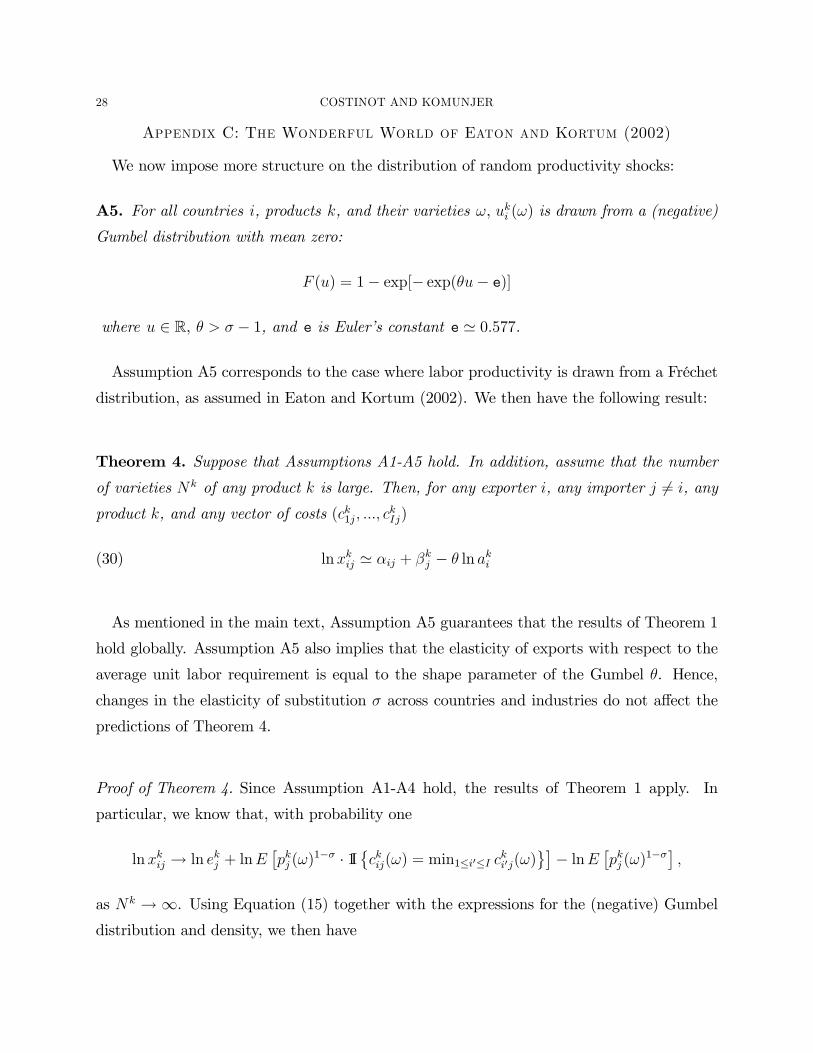
Appendix C: The Wonderful World of Eaton and Kortum (2002)
We now impose more structure on the distribution of random productivity shocks:
A5. For all countries i, products k, and their varieties !, uki (!) is drawn from a (negative)
Gumbel distribution with mean zero:
F (u) = 1� exp[� exp(�u� e)]
where u 2 R, � > � � 1, and e is Euler�s constant e ' 0:577.
Assumption A5 corresponds to the case where labor productivity is drawn from a Fréchet
distribution, as assumed in Eaton and Kortum (2002). We then have the following result:
Theorem 4. Suppose that Assumptions A1-A5 hold. In addition, assume that the number
of varieties Nk of any product k is large. Then, for any exporter i, any importer j 6= i, anyproduct k, and any vector of costs (ck1j; :::; c
kIj)
(30) lnxkij ' �ij + �kj � � ln aki
As mentioned in the main text, Assumption A5 guarantees that the results of Theorem 1
hold globally. Assumption A5 also implies that the elasticity of exports with respect to the
average unit labor requirement is equal to the shape parameter of the Gumbel �. Hence,
changes in the elasticity of substitution � across countries and industries do not a¤ect the
predictions of Theorem 4.
Proof of Theorem 4. Since Assumption A1-A4 hold, the results of Theorem 1 apply. In
particular, we know that, with probability one
lnxkij ! ln ekj + lnE�pkj (!)
1�� � 1I�ckij(!) = min1�i0�I c
ki0j(!)
�� lnE
�pkj (!)
1��� ;as Nk ! 1. Using Equation (15) together with the expressions for the (negative) Gumbeldistribution and density, we then have
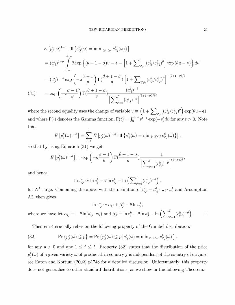
NEW RICARDIAN PREDICTIONS 29
E�pkj (!)
1�� � 1I�ckij(!) = min1�i0�I c
ki0j(!)
�= (ckij)
1��+1Z�1
� expn(� + 1� �)u� e�
h1 +
Xi0 6=i(ckij=c
ki0j)
�iexp (�u� e)
odu
= (ckij)1�� exp
��e� � 1
�
��(� + 1� �
�)h1 +
Xi0 6=i(ckij=c
ki0j)
�i�(�+1��)=�
= exp
��e� � 1
�
��(� + 1� �
�)
(ckij)��hXI
i0=1(cki0j)
��i(�+1��)=� ;(31)
where the second equality uses the change of variable v ��1 +
Xi0 6=i(ckij=c
ki0j)
��exp(�u�e),
and where �(�) denotes the Gamma function, �(t) =R +10
vt�1 exp(�v)dv for any t > 0. Notethat
E�pkj (!)
1��� = IXi=1
E�pkj (!)
1�� � 1I�ckij(!) = min1�i0�I c
ki0j(!)
�;
so that by using Equation (31) we get
E�pkj (!)
1��� = exp��e� � 1�
��(� + 1� �
�)
1hXI
i0=1(cki0j)
��i(1��)=� ;
and hence
lnxkij ' ln ekj � � ln ckij � ln�XI
i0=1(cki0j)
���:
for Nk large. Combining the above with the de�nition of ckij = dkij� wi � aki and Assumption
A2, then gives
lnxkij ' �ij + �kj � � ln aki ;
where we have let �ij � �� ln(dij� wi) and �kj � ln ekj � � ln dkj � ln�XI
i0=1(cki0j)
���. �
Theorem 4 crucially relies on the following property of the Gumbel distribution:
(32) Pr�pkj (!) � p
= Pr
�pkj (!) � p
��ckij(!) = min1�i0�I cki0j(!) ;for any p > 0 and any 1 � i � I. Property (32) states that the distribution of the price
pkj (!) of a given variety ! of product k in country j is independent of the country of origin i;
see Eaton and Kortum (2002) p1748 for a detailed discussion. Unfortunately, this property
does not generalize to other standard distributions, as we show in the following Theorem.
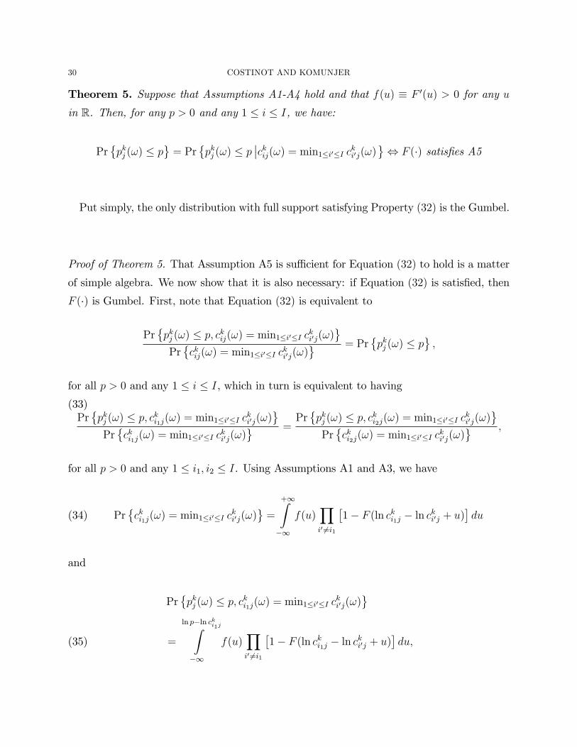
30 COSTINOT AND KOMUNJER
Theorem 5. Suppose that Assumptions A1-A4 hold and that f(u) � F 0(u) > 0 for any uin R. Then, for any p > 0 and any 1 � i � I, we have:
Pr�pkj (!) � p
= Pr
�pkj (!) � p
��ckij(!) = min1�i0�I cki0j(!), F (�) satis�es A5
Put simply, the only distribution with full support satisfying Property (32) is the Gumbel.
Proof of Theorem 5. That Assumption A5 is su¢ cient for Equation (32) to hold is a matter
of simple algebra. We now show that it is also necessary: if Equation (32) is satis�ed, then
F (�) is Gumbel. First, note that Equation (32) is equivalent to
Pr�pkj (!) � p; ckij(!) = min1�i0�I cki0j(!)
Pr�ckij(!) = min1�i0�I c
ki0j(!)
= Pr�pkj (!) � p
;
for all p > 0 and any 1 � i � I, which in turn is equivalent to having(33)Pr�pkj (!) � p; cki1j(!) = min1�i0�I cki0j(!)
Pr�cki1j(!) = min1�i0�I c
ki0j(!)
=Pr�pkj (!) � p; cki2j(!) = min1�i0�I cki0j(!)
Pr�cki2j(!) = min1�i0�I c
ki0j(!)
;
for all p > 0 and any 1 � i1; i2 � I. Using Assumptions A1 and A3, we have
(34) Pr�cki1j(!) = min1�i0�I c
ki0j(!)
=
+1Z�1
f(u)Yi0 6=i1
�1� F (ln cki1j � ln c
ki0j + u)
�du
and
Pr�pkj (!) � p; cki1j(!) = min1�i0�I c
ki0j(!)
=
ln p�ln cki1jZ�1
f(u)Yi0 6=i1
�1� F (ln cki1j � ln c
ki0j + u)
�du;(35)
NEW RICARDIAN PREDICTIONS 31
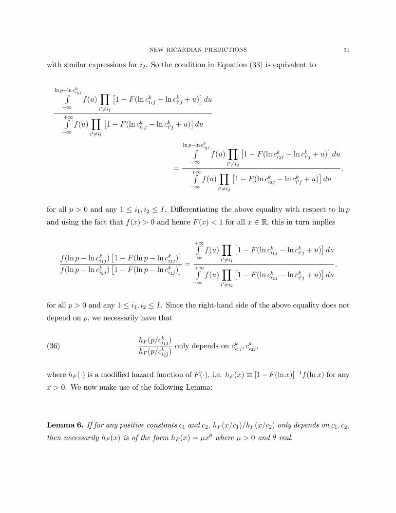
with similar expressions for i2. So the condition in Equation (33) is equivalent to
ln p�ln cki1jR�1
f(u)Yi0 6=i1
�1� F (ln cki1j � ln cki0j + u)
�du
+1R�1
f(u)Yi0 6=i1
�1� F (ln cki1j � ln cki0j + u)
�du
=
ln p�ln cki2jR�1
f(u)Yi0 6=i2
�1� F (ln cki2j � ln cki0j + u)
�du
+1R�1
f(u)Yi0 6=i2
�1� F (ln cki2j � ln cki0j + u)
�du
;
for all p > 0 and any 1 � i1; i2 � I. Di¤erentiating the above equality with respect to ln pand using the fact that f(x) > 0 and hence F (x) < 1 for all x 2 R, this in turn implies
f(ln p� ln cki1j)�1� F (ln p� ln cki2j)
�f(ln p� ln cki2j)
�1� F (ln p� ln cki1j)
� =+1R�1
f(u)Yi0 6=i1
�1� F (ln cki1j � ln cki0j + u)
�du
+1R�1
f(u)Yi0 6=i2
�1� F (ln cki2j � ln cki0j + u)
�du
;
for all p > 0 and any 1 � i1; i2 � I. Since the right-hand side of the above equality does notdepend on p, we necessarily have that
(36)hF (p=c
ki1j)
hF (p=cki2j)only depends on cki1j; c
ki2j;
where hF (�) is a modi�ed hazard function of F (�), i.e. hF (x) � [1�F (lnx)]�1f(lnx) for anyx > 0. We now make use of the following Lemma:
Lemma 6. If for any positive constants c1 and c2, hF (x=c1)=hF (x=c2) only depends on c1; c2,
then necessarily hF (x) is of the form hF (x) = �x� where � > 0 and � real.
32 COSTINOT AND KOMUNJER
Proof of Lemma 6. Let U(t; x) � hF (tx)=hF (x) for any x > 0 and any t > 0. Consider
t1; t2 > 0: we have
U(t1t2; x) =hF (t1t2x)
hF (x)
=hF (t1t2x)
hF (t1x)� hF (t1x)hF (x)
= U(t2; t1x) � U(t1; x):(37)
If the assumption of Lemma (6) holds then U(t; x) only depends on its �rst argument t and
we can write it U(t). Hence the Equation (37) becomes
U(t1t2) = U(t2) � U(t1):
So, U(�) solves the Hamel equation on R+� and is of the form U(t) = t� for some real �. Thisimplies that
(38) hF (xt) = x�hF (t):
Consider t = 1 and let � � hF (1) > 0; Equation (38) then gives
hX(x) = �x�;
which completes the proof of Lemma 6. �
(Proof of Theorem 5 continued). The result of Lemma 6 allows us to characterize the class
of distribution functions F (�) that satisfy Property (32). For any u 2 R, we have
(39)f(u)
1� F (u) = � exp(�u):
Note that when u ! �1 we have f(u); F (u) ! 0 so that necessarily � > 0. We can now
integrate Equation (39) to obtain for any u 2 R
(40) F (u) = 1� exph� exp
��u+ ln(
�
�)�i
with � > 0 and � > 0;
which belongs to the (negative) Gumbel family. Noting the expected value of the (negative)
Gumbel distribution in Equation (40) equals ���1 (ln(�=�) + e), where e is the Euler�sconstant, we necessarily have, by Assumptions A1 and A4(ii),
F (u) = 1� exp [� exp (�u� e)] with � > � � 1 for any u 2 R;
which completes the proof of Theorem 5. �
NEW RICARDIAN PREDICTIONS 33
Appendix D: Value Added per Worker
Table 3 o¤ers a snapshot of the variations in value added per worker (1=aki ) across countries
and industries in 2001, which is the latest year for which we have data on all G7 exporters.
The rankings below determine the chains of comparative advantage at the heart of the
Ricardian predictions. Broadly speaking, we see that the United States tend to have a com-
parative advantage in the pharmaceutical industry (except versus Japan) and a comparative
disadvantage in the automobile industry (except versus Italy).
Canada France Germany Italy Japan UKFood 9 1 2 4 5 4Textile 14 19 18 20 1 9Wood 18 13 17 15 2 8Paper 6 6 10 9 13 7Fuel 5 20 21 1 21 1Pharma. 2 2 1 3 16 naPlastic 11 5 11 17 11 6Minerals 12 11 7 7 8 2Iron na 14 15 11 20 naMetals na 15 19 12 18 naMetal products 13 10 8 8 3 naMachinery 15 7 13 16 10 3Computing 1 12 3 2 6 naElectrical 16 21 16 18 15 naTelecom. 4 4 5 10 14 naMedical na 9 6 5 9 naMotors 17 17 14 6 17 naBuilding 7 3 20 21 19 naAircraft 3 18 4 14 4 naTransport 10 16 12 19 12 naOther 8 8 9 13 7 5
Table 3: Rankings of Ratios of Value Added per Worker in 2001
Note: All ratios of value added per worker are computed relative to the United States. Industries are ranked from thelowest to the highest ratio.
Though we cannot report these ranking for each of the 16 years available in our sample,
we wish to point out that they are fairly stable over time. The average autocorrelation of the
di¤erence-in-di¤erence,�ln ak1i1 � ln a
foodi1
���ln ak1US � ln a
foodUS
�, is around 0:5, ranging from
0:2 in the �Aircraft and Spacecraft�to 0:7 in �Non-ferrous Metals�.
34 COSTINOT AND KOMUNJER
Appendix E: OLS estimates without US data
Variable 2003 2002 2001 2000 1999 1998 1997 1996ln a 0.67 0.65 0.88 0.77 0.69 0.86 0.93 0.67
(8.60)*** (12.23)*** (15.78)*** (15.12)*** (12.37)*** (13.06)*** (13.63)*** (9.76)***ExporterImporter FE Yes Yes Yes Yes Yes Yes Yes YesIndustryImporter FE Yes Yes Yes Yes Yes Yes Yes YesObservations 7749 14024 17319 17570 17777 17181 17225 16774R2 0.804 0.791 0.788 0.782 0.789 0.789 0.785 0.781
Variable 1995 1994 1993 1992 1991 1990 1989 1988ln a 0.76 0.71 0.47 0.47 0.37 0.34 0.37 0.08
(11.45)*** (9.13)*** (6.82)*** (6.52)*** (4.90)*** (4.64)*** (5.36)*** (1.06)ExporterImporter FE Yes Yes Yes Yes Yes Yes Yes YesIndustryImporter FE Yes Yes Yes Yes Yes Yes Yes YesObservations 16419 13244 12491 11779 10945 10775 10727 10672R2 0.7795 0.7823 0.7887 0.7903 0.780 0.778 0.776 0.776Note: Values of tstatistics in parentheses, calculated from heteroskedasticityconsistent (White) standard errors* Significant at 10% confidence level** Significant at 5% confidence level*** Significant at 1% confidence level
Table 4: YearbyYear OLS Regressions without US Data(Dependent Variable: lnx)