Embed Size (px)
Citation preview

November 18, 2003 11:17 Geophysical Journal International gji2030
Geophys. J. Int. (2003) 155, 753–777
What can GPS data tell us about the dynamicsof post-seismic deformation?
Elizabeth H. HearnDepartment of Earth and Ocean Sciences, University of British Columbia, Vancouver, BC, Canada. E-mail: [email protected]
Accepted 2003 April 22. Received 2003 February 23; in original form 2002 September 9
S U M M A R YThis paper describes differences in time-varying post-seismic deformation due to after-slipand viscoelastic relaxation following large strike-slip earthquakes, and how these differencesmay be exploited to characterize the configuration and rheology of aseismically deformingmaterial in the subsurface. The analysis involves two steps. First, near-field, time-dependentpost-seismic deformation characteristics of a typical Mw = 7.4 strike-slip earthquake is de-fined based on analysis of GPS data from three recent earthquakes. Secondly, this earthquakeis modelled (assuming uniform slip along a rectangular surface), and several classes of after-slip and viscoelastic relaxation models that can reproduce the evolution of early post-seismicdisplacements with time at a near-field reference point are developed. Postseismic displace-ments and velocities away from the reference point, where the differences are greatest (andthus most likely to be distinguished with GPS) are compared. I find that displacements froma judiciously designed network of continuous or frequently occupied campaign-mode GPSsites are sufficiently precise to distinguish linear viscoelastic relaxation from after-slip on avertical surface extending the coseismic rupture. Furthermore, both the thickness and viscos-ity of a relaxing, linearly viscoelastic layer may be identified. To maximize what post-seismicGPS surveys can tell us, particularly concerning potential relaxation of low-viscosity layersin the crust and/or upper mantle, some GPS sites should be located along strike beyond therupture tip. Also, far-field GPS sites should be occupied as frequently as sites close to therupture.
Key words: after-slip, GPS, post-seismic, viscoelastic relaxation.
1 I N T RO D U C T I O N
Major earthquakes cause static stress changes within the lithospherethat are large enough to excite observable, transient deformation ofthe Earth’s surface. Space geodetic techniques for measuring surfacedisplacements have advanced to the point where both the spatialand temporal characteristics of this post-seismic deformation canbe described in detail. This has provided geodynamic modellerswith new, powerful data sets for constraining dynamic models ofpost-seismic deformation.
Efforts to simulate deformation following recent earthquakes,however, have shown that non-unique models of the subsurface maybe consistent with post-seismic surface displacement data sets. Forexample, both after-slip and relaxation of low-viscosity lower crusthave been put forward to explain long-wavelength, rapidly decay-ing crustal deformation during the first 6 months after the 1992Landers, California earthquake (Shen et al. 1994; Yu et al. 1996).Later deformation (6 months to 7 yr after the earthquake) has alsobeen explained with different after-slip and viscoelastic relaxationmodels (e.g. Savage & Svarc 1997; Deng et al. 1998; Freed & Lin2001; Pollitz et al. 2001).
Some of this non-uniqueness arises from calibrating models todifferent displacement fields, even when GPS data from the samesources are used. Differences can result from using data from dif-ferent groups of GPS sites; including or neglecting inSAR rangechanges in the analysis; focusing on different time intervals, or ap-plying different corrections for secular deformation. Another reasonfor the lack of consensus among Landers post-seismic deforma-tion models is that differences in displacement patterns producedby various processes may be small, relative to GPS measurementerrors. Still, resolving the cause of post-seismic deformation is im-portant: after-slip or viscoelastic relaxation of materials distributedin various ways in the crust may stress the crust and upper mantlein significantly different ways while producing comparable surfacedeformation (Hearn et al. 2002).
With the recent funding of the Plate Boundary Observatory (PBO)and the Southern California Earthquake Center (SCEC II), increas-ingly detailed measurements of surface deformation will be col-lected following future earthquakes in western North America. Inlight of this, we need to ask some fundamental questions, namely:(1) can after-slip and viscoelastic relaxation of horizontal layersbe distinguished from each other with GPS data, given typically
C© 2003 2003 RAS 753

November 18, 2003 11:17 Geophysical Journal International gji2030
754 E. H. Hearn
0
5
10
8
4
0
4
0 50 100 150
LDES
LDSW
20
10
0
10
5
0
5
0 50 100 150
Time (days)
Nor
th (
mm
)E
ast
(mm
)N
orth
(m
m)
Eas
t (m
m)
Time (days)
Figure 1. Horizontal displacements as a function of time, from GPS sites near the Hector Mine (LDES and LDSW), Landers (LAZY and PAXU) and Izmit(TUBI and DUMT) earthquake ruptures.
available coverage and measurement precision and if so, (2) howshould we monitor post-seismic deformation to maximize the like-lihood of differentiating between competing models?
To address these questions, I develop several after-slip and vis-coelastic crust or mantle relaxation models that reproduce time-dependent post-seismic displacements typical of recent major strike-slip earthquakes at a near-field reference point. I show that spatialpatterns and temporal evolution of post-seismic displacements pre-dicted by these models differ, and point out how they can be dis-tinguished from each other with space geodetic data. I also sug-gest how GPS networks monitoring post-seismic deformation fol-lowing large strike-slip earthquakes should be designed to maxi-mize what they can tell us about the structure and rheology of thelithosphere.
2 S U R FA C E D E F O R M AT I O N F RO MM A J O R E A RT H Q UA K E S O NS T R I K E - S L I P FAU LT S
This paper focuses on early post-seismic deformation because it isat this time, when surface velocities and accelerations are highest,that we have the best chance of precisely characterizing the tem-poral evolution and spatial pattern of this transient deformation. AtGPS sites where frequent, high-precision data are available, a de-
caying transient with a characteristic decay time (τ c) of 30–80 dcan often be identified in at least one horizontal motion component(e.g. Shen et al. 1994; Savage & Svarc 1997; Ergintav et al. 2002;Owen et al. 2002) following large strike-slip earthquakes. This isapparent in the displacement–time curves shown on Fig. 1, and onadditional data plots from Shen et al. (1994), Savage & Svarc (1997),Ergintav et al. (2002) and Owen et al. (2002). Similar episodes oftransient surface deformation follow subduction zone earthquakes(Webb & Melbourne 1996; Heki et al. 1997) and shallow thrustfaulting events (Hsu et al. 2002). The rapidly decaying transientdeformation is superimposed on a more slowly decaying deforma-tion transient (Bock et al. 1997; Savage & Svarc 1997), which maycontain some contribution from the τ c = 20–100 yr decaying de-formation mode identified from post-1906 San Andreas earthquakestrain data (Thatcher 1983; Kenner & Segall 2000).
Since the first part of this study involves developing models thatproduce near-field post-seismic deformation typical of a Mw = 7.4strike-slip earthquake, a reference point for comparisons betweenmodelled and ‘typical’ (observed) post-seismic displacements mustbe chosen. For the earthquake model described below, I define a pointlocated on a perpendicular line bisecting a hypothetical, rectangularearthquake rupture and at a distance of 15 km from the rupture asthe reference point, ‘Station A’ (Fig. 2). For a planar rupture withuniform slip, azimuths at this location will not vary over time and no
C© 2003 RAS, GJI, 155, 753–777

November 18, 2003 11:17 Geophysical Journal International gji2030
Dynamics of post-seismic deformation 755
0 400 800 1200 1600 2000
-20
-10
0
0
50
100
0
20
40
0102030
Nor
th (
mm
)E
ast
(mm
)N
orth
(m
m)
Eas
t (m
m)
PAXU
LAZY
Time (days)
Time (days)
0 400 800 1200 1600 2000
Figure 1. (Continued.)
vertical motion will occur, so comparing model results to the Sta-tion A displacement–time curve is less complicated than it would beif Station A were in another location. Another reason for choosingthis near-field location as a reference point is that post-seismic GPSsurveys have historically concentrated on sites close to the earth-quake rupture, so more GPS data are available in this area. The nextsection describes how a ‘typical’ post-seismic displacement–timecurve for Station A was inferred from GPS observations followingthree recent earthquakes.
2.1 Individual earthquakes
‘Typical’ post-seismic displacements at reference Station A within1 yr of a Mw = 7.4 strike-slip earthquake are based on an analy-sis of GPS data from the 1999 Izmit, Turkey; 1999 Hector Mine,California; and 1992 Landers, California earthquakes. In the follow-ing sections, I describe post-seismic surface deformation followingeach of these earthquakes, and then discuss how these data wereused to arrive at the station a displacement–time curve.
2.1.1 1992 Landers, California earthquake
The SCEC and the USGS GPS networks in southern California(e.g. Shen et al. 1994; Savage & Svarc 1997) provide 7 years of
measurements of post-seismic deformation triggered by the 1992Landers earthquake (i.e. up to the time of the 1999 Hector Mineearthquake). These data have been combined, placed in a stableNorth America reference frame, and reprocessed together using theGAMIT and GLOBK GPS data processing packages. The post-seismic displacement–time data were corrected for contributionsfrom secular deformation, which were estimated using an elasticblock model (Souter 1998; McClusky et al. 2001). The east andnorth displacement components (Et and N t) were then fitted tofunctions with exponential and linear components:
Et = Eexp
(1 − e−t/τ
) + Elin
(t
365
)(1)
Nt = Nexp
(1 − e−t/τ
) + Nlin
(t
365
), (2)
where E exp, E lin, N exp and N lin are amplitudes of the exponentialand linear components. Overall, exponential decay times (τ c) of80–200 d fit the data best, but the sensitivity of the misfit to τ c
is low for sites that were surveyed infrequently. When I fix τ c at80 d (consistent with Savage & Svarc 1997), the normalized rmsvalues fall within the 95 per cent confidence interval of χ 2 for thenumber of degrees of freedom at each site (i.e. the number of ob-servations). The fit of the data-fitting functions (eqs 1 and 2) to the
C© 2003 RAS, GJI, 155, 753–777

November 18, 2003 11:17 Geophysical Journal International gji2030
756 E. H. Hearn
3020100
0 50 100 150 200 250 30060
40200
Nor
th (
mm
)E
ast (
mm
)
Time (days)
0 50 100 150 200 250 300
20
10
0
0
20
40
TUBI
DUMT
Nor
th (
mm
)E
ast (
mm
)
Figure 1. (Continued.)
Figure 2. Modelled strike-slip rupture (plan view, one quadrant) and loca-tions of hypothetical GPS stations A–G where displacements are calculated.
east and north displacements is shown for near-field sites LAZYand PAXU in Fig. 1. Although resolution of the decay time is poorfor many (less frequently monitored) sites, they clearly require adecaying velocity transient in at least one horizontal direction (usu-ally the north component). At these sites, even where the decay time
is not well resolved, errors in the estimated amplitude of the de-caying transient are generally less than 20 per cent. At some sites,the data are insufficient to resolve whether a decaying transient ispresent or not. In these locations, estimates of τ c (usually of theorder of hundreds of days) are associated with large errors (i.e.a 1σ error equal to the estimated decay time or greater). Fig. 3shows the amplitudes of the exponential and linear terms compris-ing the displacement–time curve that best fits the horizontal GPSdisplacement magnitudes (At) at each site, plotted against distancefrom the rupture. The amplitudes of these terms ( Aexp and Alin) arenormalized to the horizontal, coseismic site displacement (Ac). Atsites where coseismic displacements were unavailable (for all threeearthquakes), Ac was estimated using an elastic dislocation model.The equation for horizontal post-seismic displacement at each GPSsite is
At = Ac
[Aexp
(1 − e−t/τ
) + Alin
(t
365
)]. (3)
I should note here that the early post-seismic velocities are de-scribed as decaying exponentially with time simply because it isconvenient. Describing the displacement–time curves with expo-nential functions is not meant to imply that viscoelastic relaxationis the cause rather than after-slip (which can produce logarithmicvelocity decay in the near field; Marone et al. 1991). Furthermore,
C© 2003 RAS, GJI, 155, 753–777
November 18, 2003 11:17 Geophysical Journal International gji2030
Dynamics of post-seismic deformation 757
0 0.1 0.2 0.3 0.4 0.5 0 0.1 0.2 0.3 0.4 0.5
0 10 20 30 40 50 0 10 20 30 40 500
5
10
15
20
25
0
5
10
15
20
25
0
5
10
15
0
5
10
15
exp
Aex
pA
linA
linA
Distance from rupture (km) Distance from rupture (km)
Distance from rupture /L Distance from rupture /L
(a) (b)
(c) (d)
Figure 3. Aexp and Alin for individual GPS sites following the Hector Mine, Landers and Izmit earthquakes. Black, grey and open circles represent data fromthe Landers, Hector Mine and Izmit earthquakes, respectively. Top (a and b): Aexp and Alin plotted against distance from the rupture. Bottom (c and d): Aexp
and Alin plotted against normalized distance to the fault (i.e. distance/rupture length L). Available data for the Izmit and Hector Mine events covered shortertime intervals (300 and 140 d, respectively) than data from the Landers earthquake (2200 d), leading to larger errors in the estimates of Aexp and Alin. Thus,only data from continuous GPS sites are shown for the former two earthquakes.
analytical solutions for 2-D models of a dislocation in an elasticlayer over a viscoelastic half-space represent the evolution of sur-face displacements with time as an infinite sum of exponentials withdifferent decay times and amplitudes (e.g. Nur & Mavko 1974; Rice1980; Pollitz 1997; Cohen 1999). Only at sites very close to the faultdoes a single exponential term dominate.
2.1.2 1999 Hector Mine, California and Izmit, Turkey earthquakes
Post-seismic displacement data from the first 6 months followingthe Hector Mine earthquake were processed and fitted to the data-fitting function (eq. 3) as described above for the Landers earth-quake. As with the Landers data, horizontal displacement compo-nents from some sites showed decaying velocities that could be fittedwith eqs (1) and (2) (e.g. sites LDES and LDSW in Fig. 1). Datafrom sites that were not frequently occupied, or that were far fromthe rupture, are fitted equally well without an exponential term. De-cay times of 20–80 d were preferred by displacement data where anexponential term was required. When I fix τ c at all sites to 40 d, thenrms values fall within the 95 per cent confidence interval of χ2 forthe number of degrees of freedom at each site (i.e. the number ofobservations). Resolution of the decay time is poor at most of thecampaign-mode GPS sites, but errors in the estimated amplitude ofthe decaying transient are generally less than 20 per cent. For eachsite, Aexp and Alin are plotted against distance to the rupture in Fig. 3.Post-seismic displacements for the first 300 d following the Izmitearthquake have also been fit with summed exponential and linearfunctions (Ergintav et al. 2002) and τ c is about 60 d. Before the
analysis was done, the GPS data were corrected for displacementsassociated with the nearby Duzce earthquake, which occurred 87 dafter the Izmit earthquake. The data from Ergintav et al. (2002) werealso corrected for secular velocities using velocities from a blockmodel (Meade et al. 2002) and, where available, pre-Izmit velocitydata (McClusky et al. 2000). The fit of eqs (1) and (2) to the east andnorth displacements is shown for near-field sites TUBI and DUMTin Fig. 1. For each GPS site, Aexp and Alin are plotted against distanceto the rupture in Fig. 3.
2.2 Synthetic, near-field post-seismic displacementsversus time
For each earthquake, representative values of Aexp and Alin at Sta-tion A were estimated by least-squares fitting a line to plots of theseparameters against distance from the rupture (Fig. 3) and interpo-lating their magnitudes at 0.25L . In absolute length, 0.25L is 11,16 and 25 km for the Hector Mine, Landers and Izmit earthquakes.Fig. 3 shows the magnitude of Aexp and Alin for sites within half arupture length (i.e. 0.5L) of each fault, plotted against the distancebetween the site and the rupture. For each earthquake, magnitudesof the exponential and linear (velocity) terms correlate with dis-tance to the fault: correlation coefficients range from 0.61 to 0.76.For the Landers earthquake, the exponential term magnitude was 5per cent of the coseismic displacement, and the velocity term was1.5 per cent of the coseismic displacement per year. Similar resultsare obtained from the Hector Mine earthquake data. Data from theMw = 7.5 Izmit earthquake seem to require a larger Aexp, but the
C© 2003 RAS, GJI, 155, 753–777
November 18, 2003 11:17 Geophysical Journal International gji2030
758 E. H. Hearn
Dis
plac
emen
t / c
osei
smic
0
0.05
0.1
0.15Station A
1 σ range
Time (days)
0 12060 180
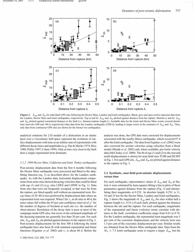
Figure 4. Curve fit to displacement–time data from GPS sites within adistance of L/2 of each of the three earthquake ruptures. The hypotheticalStation A displacement–time curve is superimposed (heavy black line). Theshaded area brackets the plus or minus 50 per cent interval for the Station Adisplacement–time curve.
displacement–time data at many of the sites do not cover a longenough time interval to properly separate the (τ c ≥ 80 d) exponen-tial term from the linear term.
Since the longest-duration post-seismic displacement data set isfrom the Landers earthquake, I model an earthquake of comparablemagnitude (Mw = 7.4) and use the Landers data to define Alin. Aexp
for Station A is an average of its values for the three earthquakes,which is equal to its value for the Landers earthquake alone. Themodelled coseismic displacement at Station A due to the referenceMw = 7.4 strike-slip earthquake (described below) is 0.52 m, so theamplitude of the decaying transient and the long-term velocity are 26and 8 mm yr−1, respectively. Fig. 4 shows the Station A displacementversus time curve, together with displacement versus time curves forGPS sites located within half a rupture length of each earthquake.The Station A curve appears to be representative of near-field, post-seismic deformation following all three earthquakes: at any giventime, displacements at most of these GPS sites are within 50 percent of the Station A displacement.
2.3 ‘Typical’ data errors
Since one point of this project is to evaluate whether differences insurface displacements produced by various post-seismic processescan be discerned with GPS data, ‘reasonable’ errors associated withthese measurements must be defined. The precision of campaign-mode GPS measurements of post-seismic displacements is highlyvariable, and depends on the frequency and duration of occupations,how soon after the earthquake displacement measurements weremade, and on the duration of position monitoring at the site prior tothe earthquake (i.e. how well the pre-earthquake velocity of the sitewas known). GPS sites that were operating prior to an earthquake,and which are monitored frequently (i.e. at least weekly) may mea-sure post-seismic displacements to within a 1σ error (68 per centconfidence interval) of 1 mm (T. Herring, personal communication,2001). However, GPS networks designed to observe post-seismicdeformation often include many sites where pre-earthquake veloc-ities are not known, and frequent monitoring during the first few
weeks after an earthquake is often not possible because of logisticalchallenges. I will assume 1σ errors of 3 and 1 mm, respectively, arepossible at campaign-mode and continuous GPS sites, respectively.These are comparable to many of the 1σ errors for post-seismic dis-placements following the Izmit and Hector Mine earthquakes (e.g.Fig. 1; Ergintav et al. 2002; Owen et al. 2002), and measurementprecision (under optimal circumstances) continues to improve withtime. Vertical displacement estimates from GPS are associated withlarger errors than horizontal displacement estimates. A typical 1σ
measurement error for a Landers earthquake, post-seismic verticaldisplacement is 10 mm (e.g. Savage & Svarc 1997). Smaller errors(3–5 mm) should be possible at continuous stations (T. Herring, per-sonal communication, 2001) though for the Izmit and Hector Mineearthquakes, most errors in vertical position estimates at continuousGPS sites were considerably larger. InSAR range change measure-ments may provide vertical displacement estimates if horizontalcontributions to range change can be removed. However, even if aperfect correction for horizontal contributions is possible, 1σ errorsassociated with inSAR vertical displacement estimates should beof the order of a centimetre. Because of difficulties associated withobtaining precise measurements of post-seismic vertical displace-ments, most of the discussion in the following sections concernshorizontal displacements.
3 M O D E L L I N G M E T H O D
3.1 Viscoelastic finite-element code
I model coseismic and post-seismic deformation using a viscoelasticfinite-element code developed specifically for geological applica-tions (Saucier et al. 1992; Saucier & Humphreys 1993). This code(GAEA) models 3-D, time-dependent displacements and stressesthroughout a volume due to imposed boundary conditions and/orfault slip. Because GAEA incorporates quadratic block elements,curvilinear fault surfaces with smoothly varying slip may be rep-resented. Stresses on these surfaces (which lie along interfaces be-tween elements and are typically interpolated) may also be estimatedwith a precision greater than that possible for models incorporatinglinear shape functions and similar nodal spacing.
I have run several elastic and viscoelastic test models to comparethe performance of GAEA with that of other programs. Coseismicdisplacements from a Mw = 7.4 strike-slip earthquake (describedbelow) were calculated using GAEA, TEKTON 2.2 (Melosh &Raefsky 1981) and 3D-DEF (Gomberg & Ellis 1994). Elastic sur-face displacements for GAEA, TEKTON and 3D-DEF are in agree-ment throughout the modelled region to within about 2 per cent,except within a few kilometres of the fault tip (i.e. within lessthan one model element dimension) and beyond two fault lengthsfrom the modelled rupture, where amplitudes are less than about0.5 mm.
For a viscoelastic lower-crust model, I compared post-seismicdisplacements that were calculated using GAEA, TEKTON 2.2(Melosh & Raefsky 1981) and VISCO1D (Pollitz 1997). The mod-els produced similar patterns and magnitudes of surface deforma-tion within about 100 km of the fault over 1 year (six Maxwelltimes). As a result of fixed boundary conditions, GAEA and TEK-TON yield more pronounced decay in amplitudes with distancethan VISCO1D, but vector azimuths, vertical displacement pat-terns and time-dependent changes in velocities and azimuths aresimilar.
To dynamically model after-slip, GAEA calculates shear stressesacting on planes tangent to the fault surface at each fault node,
C© 2003 RAS, GJI, 155, 753–777

November 18, 2003 11:17 Geophysical Journal International gji2030
Dynamics of post-seismic deformation 759
and calculates slip rates for each time step based on either velocity-strengthening friction or viscous flow laws (described in subsequentsections). Though frictional and viscous properties are specified ateach nodal position and may vary spatially, I restrict this study tofaults or shear zones with depth-varying properties. To model non-linear viscoelastic relaxation, GAEA calculates deviatoric stress(σ 1 − σ 3) at the centre of each model element and uses this stressto calculate the effective viscosity of the element at the start of eachtime step.
GAEA inverts for parameters by either a grid search or a MonteCarlo approach, selecting the parameter set that minimizes thesquared residual between the posited Station A displacements(Fig. 4) and modelled displacements, summed over 36 10 d intervals(i.e. 1 yr).
Gravitation is not incorporated in these models. For models withlinearly viscoelastic layers, gravitation may perturb vertical dis-placement solutions if t > 50T M (Pollitz 1997), where T M, orMaxwell time, is viscosity (η) divided by shear modulus (G). Post-seismic displacements presented in this paper are calculated for t <
25T M.
3.2 Model mesh
The model mesh covers a region of 520 × 520 × 250 km3, and iscentred on a N–S oriented, vertical rupture. The planar rupture is65 km long and extends from the free surface to a depth of 15 km. 3 mof right-lateral, horizontal slip is imposed along this surface using‘split nodes’ (Melosh & Raefsky 1981). The modelled volume is aPoisson solid with a Young’s modulus (E) of 70 GPa.
The base and sides of the modelled volume are fixed, and thetop surface is unconstrained. To make sure this choice of boundaryconditions was reasonable, I evaluated the effect of the fixed basaland side boundaries on coseismic and post-seismic stresses anddisplacements. Comparing elastic models with stress-free and fixedbasal boundaries, I found the difference to horizontal shear stressesresolved on to fault nodes to be less than 5 per cent down to depths ofup to 150 km, and effects on surface displacements were negligible.Modelling the side boundaries as fixed or unconstrained, I found thathorizontal surface displacements up to 150 km from the rupture tracematched to within about 5 per cent, and that fault zone stresses werenearly identical at all depths. The largest differences in coseismicdisplacements and fault surface stresses were in the far field and atdepth, where their magnitudes were low (less than a millimetre and0.001 MPa, respectively).
I also evaluated the effect of fixed bottom and side boundaryconditions on post-seismic surface displacements and stresses after1 yr (six Maxwell times), using a viscoelastic lower-crust model.Results from a version of this model with fixed side and bottomboundaries were compared with results from a version with uncon-strained boundaries on the bottom and the two sides bounding thequadrant in which stresses and displacements were calculated. Post-seismic surface displacements from the two models differ by lessthan 2 per cent within 100 km of the rupture. The relative differencesin far-field displacements are greater, but both models indicate totalpost-seismic displacements after 1 yr of less than 0.5 mm (i.e. notdetectable with GPS) in these areas.
3.3 Post-seismic deformation models
Each of the models in this paper focuses on a single process, suchas after-slip or relaxation of a particular low-viscosity layer. This
process is not responsible for all aseismic deformation along a plateboundary throughout the earthquake cycle: to connect the relativemotion of two sides of a fault to relatively steady relative platemotions at depth, aseismic processes must occur from the seismo-genic zone to the upper mantle. For example, if frictional after-slipis responsible for early post-seismic deformation, a second, sloweraseismic process (such as viscoelastic relaxation of the lower crust ora deep extension of the shear zone) must accommodate the relativeplate motion between the Moho and the middle crust. The modelsdescribed below address only the most rapidly occurring aseismicdeformation process.
3.3.1 Viscoelastic layers
In models incorporating, viscoelastic layers or the elastic upper crustthickness, H , as well as the viscosity (η) and thickness (h) of theviscoelastic layer, are varied.
For the linear viscoelastic models (groups 1A, 1B and 1C), elasticcrust thicknesses (H) of 15, 25 and 33 km, respectively, are mod-elled (Table 1). Since the base of the rupture is always at 15 kmdepth, this means the fault penetrates 100, 60 or 45 per cent ofthe elastic layer. Within each of these groups, four different valuesof viscoelastic layer thickness (h) and several viscosity values aremodelled.
Viscoelastic relaxation of crust or mantle layers with non-linearrheology (group 2A and 2B models) is modelled assuming a stressexponent (n) of 3. I parametrize the non-linear behaviour rather thanforward modelling specific flow laws, which would be a less efficientway to match the Station A displacements. Non-linear flow laws forrocks comprising the crust and mantle are generally of the form
ηeff = µn
Aσ n−1exp
(E∗ + PV ∗
RT
). (4)
In eq. (4), E∗ is the activation energy, P is the pressure, T is thetemperature, µ is the shear modulus, V ∗ is the activation volume,R is the gas constant, A is an empirically determined constant, σ
is the differential stress (σ 1 − σ 3) and ηeff is the effective viscos-ity. These parameters vary dramatically with rock type and volatilecontent, and these are not well constrained for the lower continen-tal crust. Furthermore, eq. (4) requires σ as an input, but absolutevalues of lower crustal stresses are not known. Rather than guessingreasonable compositions and stresses to calculate ηeff directly usingeq. (4), my approach is to determine what the parameters in eq. (4)would have to be in order to reproduce near-field, early post-seismicdeformation typical of large earthquakes. Since
ηeffσn−1 = constant (5)
non-linear flow laws may be parametrized with a pre-earthquakedifferential stress (σ pre), a pre-earthquake effective viscosity (ηpre),and a stress exponent n (assumed to be 3):
ηeff(t,elem) = ηpre
[σpre
σpre + σ(t,elem)
]2
(6)
where ηeff(t,elem) and σ (t,elem) are the effective viscosity and the dif-ferential stress (coseismic plus post-seismic) in the model elementat time t after the earthquake. Since σ (t,elem) is calculated by thefinite-element code prior to each time step, and n = 3, the only freeparameters are ηpre and σ pre, which are randomly sampled from awide range of permissible values. The group 2A and 2B modelsdo not take depth variation of ηpre and σ pre into account. ηeff(t,elem)
drops at the time of the earthquake because of the coseismic element
C© 2003 RAS, GJI, 155, 753–777

November 18, 2003 11:17 Geophysical Journal International gji2030
760 E. H. Hearn
Table 1. Summary of optimal model input parameters, and the misfit to the Station A displacement–time curve. The misfit is reportedas WRSS, which is the sum over 36 10 d intervals of the square of the misfit in each horizontal displacement component divided byreasonable measurement errors (2 mm). Note that there is no vertical displacement at Station A because of its location along a nodalsurface separating compressional and dilational quadrants (i.e. no poloidal contribution).
Group H (km) h (km) η (Pa s) T E (d) T M (d) WRSS (m2)
Linear viscoelastic models1A 15 2 3.2 × 10¹⁷ 580 120 0.001
15 15 1.9 × 10¹⁸ 450 740 0.00215 30 1.9 × 10¹⁸ 380 1000 0.00215 125 2.6 × 10¹⁸ 80 960 0.002
1B 25 2 4 × 10¹⁶ 120 16 0.000 1325 8 2 × 10¹⁷ 90 61 0.000425 25 4 × 10¹⁷ 110 200 0.00225 115 6.4 × 10¹⁷ 41 250 0.002
1C 33 3 1.3 × 10¹⁶ 13 2 0.000 2833 17 1017 35 30 0.000 0433 52 1.3 × 10¹⁷ 30 77 0.000 2733 107 1.4 × 10¹⁷ 19 100 0.000 32
Group H (km) h (km) η0 (Pa s) σ ′n (MPa) n WRSS (m2)
Non-linear viscoelastic models2A 15 17 1021 0.02 3 0.000 252B 33 107 1.2 × 10¹⁹ 0.0014 3 0.0016
Group z (km) η0/w (Pa s m−1) zd WRSS (m2)
Viscous afterslip models3 15 4 × 10¹⁵ 2.1 0.0005
Group z (km) (a − b) v0 (mm yr−1) σ ′eff (MPa km−1) WRSS (m2)
Frictional afterslip models4 15 0.000 36 2 20 7.3 × 10⁻⁵
15 0.000 72 10 20 3.4 × 10⁻⁵
15∗ 0.001∗ 10∗ 20∗ 0.000 59∗15 0.000 55 20 20 4.1 × 10⁻⁵
∗Without tapered slip; see text.
stress increase, then gradually increases toward its pre-earthquakevalue (ηpre). Eq. (6) illustrates that unless the coseismic stressσ (t,elem) is of the order of σ pre, the coseismic change to ηeff may bemodest.
Mid- to lower crust (between 15 and 33 km depth) deformingwith non-linear rheology is represented by the group 2A models. Thegroup 2B models represent a non-linearly viscoelastic upper-mantlelayer 33–140 km below the surface. In the results section, I discusswhether parameters required by the most successful non-linearlyviscoelastic models are consistent with temperatures, stresses androck compositions typical of continental lower crust or uppermantle.
3.3.2 Vertical shear zones
Shear zones extending downward from the seismogenic rupture areoften idealized as creeping via stable frictional slip in the middlecrust and via viscous creep at greater depths. For this project, I as-sume that one or the other of these processes is dominant early afteran earthquake, so I model each type of after-slip separately. Dur-ing each time step, horizontal shear stresses resolved on to planestangent to the fault surface are calculated at each node, and a consti-tutive relationship is used to calculate the horizontal slip increment.This slip increment is added to the cumulative slip displacement foreach split node and the summed slip is imposed for the followingtime step. In the after-slip models, all model layers are assumedto behave elastically, and after-slip may occur from the base of thecoseismic rupture downward.
Velocity-dependent frictional after-slip (group 3 models) may beeither stable or unstable, depending on the properties of the faultsurface, temperature and other parameters. The change in frictioncoefficient with slip velocity is parametrized with the value (a −b). If (a − b) is positive, the fault zone is velocity strengtheningand slip is stable. If (a − b) is negative, the fault zone is velocityweakening and stick–slip behaviour occurs. Slip during each timestep is calculated using the following equation (Marone et al., 1991,from the equations of Dieterich (1979) or Ruina (1983)).
ds = dtV0 exp
[dτ
(a − b)σ ′n
]. (7)
V 0 is the secular slip rate, (a − b) is the empirical constant relat-ing fault friction change to change in slip velocity, σ ′
n is the effectivenormal stress, ds is the slip per time step, τ is the time-dependentearthquake-induced shear stress resolved on to the fault surface, anddt is the time step length. This equation assumes that the steady-statevalue of (a − b) has been attained wherever after-slip is modelled,and does not evolve with early slip. The parameter (a − b) is var-ied, and effective normal stress σ ′
n is held constant at 20 MPa km−1
depth. This method for modelling stable frictional after-slip is anal-ogous to the ‘hot friction’ model of Linker & Rice (1997), whomodelled aseismic slip following the 1989 Loma Prieta, Californiaearthquake.
For viscous shear zone creep (group 4 models), the ‘slip’ (i.e.shear strain integrated across the shear zone) per time step is
ds = dτ
(η/w)dt. (8)
C© 2003 RAS, GJI, 155, 753–777

November 18, 2003 11:17 Geophysical Journal International gji2030
Dynamics of post-seismic deformation 761
In eq. (8), η is viscosity, w is the horizontal width of the shearzone and the parameter η/w is varied. In crustal rocks, η shoulddecline with increasing temperature and be only mildly sensitive topressure, and thus should decrease with depth (z) in compositionallyuniform crust. However, the rheology of the lower crust is proba-bly controlled by feldspar rather than quartz, causing a viscosityincrease in the lower crust. Also, the ratio of fault zone viscosity tothat of its surroundings may decrease with depth, causing the shearzone to widen; such a widening of exhumed shear zones with depthis seen in field studies (e.g. Hanmer 1988). This widening wouldoppose a decrease in η/w (or (η/w)z) with depth. Because of theseuncertainties on how shear zone properties vary with depth, I fo-cus on models in which (η/w)z is either uniform or decreases withdepth. (Models with depth-increasing (η/w)z would yield after-slipconcentrated just below the rupture, similar to the group 3 models.)The decrease in (η/w)z with depth is modelled as follows:
( η
w
)z=
( η
w
)0
exp
(z − 15
zd
). (9)
In this equation, z is the depth in kilometres, zd is a decay param-eter and (η/w)0 is the viscosity divided by the shear zone width at15 km depth.
For both classes of vertical shear zone models, after-slip may oc-cur wherever the fault zone was coseismically loaded by the earth-quake, except in the top 15 km of the crust (where the fault was co-seismically loaded beyond ends of the rupture). This last assumptionis based on the fact that little or no after-slip occurred in the uppercrust beyond the tips of the Izmit or Landers earthquake ruptures(e.g. Reilinger et al. 2002; Shen et al. 1994). Frictional after-slipdid occur on the Izmit rupture surface itself (Hearn et al. 2002), butfor the uniform slip case modelled here, no part of the rupture iscoseismically loaded, as patches of low coseismic slip on the Izmitrupture surface were.
4 R E S U LT S
4.1 Models consistent with typical near-field (Station A)post-seismic displacements
4.1.1 Newtonian viscoelastic crust or mantle layers
Several viscoelastic models can approximately reproduce the Sta-tion A displacement–time curve (Fig. 5). To reproduce both theamplitude and the decay behaviour, the relaxing layer must be lo-cated at depth below the base of the earthquake rupture, and musthave a low value of η. Many models from groups 1B and 1C fit theStation A displacement history to within a mean of less than 3 mmper epoch (i.e. the campaign-mode GPS 1σ error under optimal con-ditions). For the best group 1B and 1C models (VE-1B and VE-1C),the summed, squared residuals (SSRs) are 1.3 × 10⁻⁴ and 4.2 ×10⁻⁵ m2, respectively, consistent with a mean misfit per 10 d epochof 2.5 and 1 mm. (For comparison, a model with zero displacementat any time yields an SSR of 0.024 m2, the best-fitting straight lineyields an SSR of 0.0022 m2 and curves within the shaded regionin Fig. 4 yield SSRs of up to 0.012 m2.) For each model group,sensitivity of the SSR to variations in model parameters is shown inFig. 6.
The best group 1B model, VE-1B, requires a viscosity of 4.0 ×10¹⁶ Pa s at 25–27 km depth. One measure of characteristic stressrelaxation time in models with thin viscoelastic layers is the Elsasser
Newtonian viscoelastic
Nor
th (
mm
)
0
10
20
30
40
50
VE_1A
VE_1BVE_1C
0
10
20
30
40
Nor
th (
mm
)
50nonlinear viscoelastic (n=3)
VE_2A
VE_2B
0
10
20
30
40
Nor
th (
mm
)
Afterslip or shear zone creep
Time (days)
VC
FS
FS (tapered)
50
0 100 200 300 400
Figure 5. Modelled displacements versus time at Station A for severalclasses of viscoelastic relaxation and after-slip models. Top, middle andbottom figures show results from Newtonian viscoelastic, non-linear vis-coelastic and after-slip models with parameters optimized to best fit the Sta-tion A displacement–time curve from Fig. 4. See the text for a descriptionof each model.
time (T E), which is calculated as follows (Lehner et al. 1981):
TE = TMcH
h, (10)
where c is (π/4)2 and T M (Maxwell time) is η /µ. For model VE-1B,T E is 120 d. For the group 1C models, the best fit to the Station Adisplacements is obtained with a viscoelastic layer extending from33 to 50 km depth with a viscosity of 1017 Pa s or T E ≈ 35 d. Thismodel (VE-1C) is somewhat analogous to viscoelastic upper-mantlemodels proposed by Pollitz et al. (2001). In model VE-1C, however,the lower crust is modelled as elastic rather than as a standard linearsolid, the lowest-viscosity mantle layer is much thinner, and there isno high-viscosity layer immediately below the crust.
None of the group 1A models can adequately reproduce the Sta-tion A displacement–time curve. Though the near-field post-seismicdata (Fig. 3) allow a wide latitude for acceptable models, a decayingvelocity with a τ c of about 80 d and a total displacement of tens ofmm after 1 yr are required. The group 1A models yield excessive
C© 2003 RAS, GJI, 155, 753–777

November 18, 2003 11:17 Geophysical Journal International gji2030
762 E. H. Hearn
17.5 18 18.5log effective viscosity
5
10
15
20
25
laye
r th
ickn
ess
(km
) 0.01
0.02
0.03
0.005
0.03a
log effective viscosity
5
10
15
20
laye
r th
ickn
ess
(km
)
16.5 17 17.5 18
0.03
0.02
0.03
0.01
0.01
0.005
b
17 17.5 18log effective viscosity
10
15
20
25
30
35
40
laye
r th
ickn
ess
(km
)
0.005
0.010.02
0.01
0.02
c
3.4 3.2 3 2.8log (a-b)
4
6
8
10
12
14
16
18
Vo
mm
yr−
1
0.01
0.01
0.005
0.005
0.001
0.0010.02
d
14 14.5 15 15.5log viscosity/width Pa s km−1
1.5
2
2.5
3
Dec
ay p
aram
eter 0.005
0.01
0.010.02
0.02
0.03
e
19 19.5 20 20.5
4.5
5
5.5
log initial effective viscosity
log
initi
al s
tres
s (
Pa)
0.005
0.01
0.005
0.01
0.03
f
Figure 6. Sensitivity of model misfit to free parameters. Squared residuals between modelled displacements and the Station A displacement–time curve (Fig. 4)are summed over 36 10 d time intervals. (a)–(c) Group 1A, 1B and 1C linear viscoelastic models. (d) Group 3 (frictional after-slip) models, (e) group 4 (viscousshear zone creep) models, (f) group 2 (non-linear viscoelastic lower crust) models. Dots show the location in parameter space where the SSR is minimized. Forcomparison, a model in which Station A did not move would have an SSR of 0.024 m2, and the best-fitting line has an SSR of 0.0022 m2. Displacement–timecurves within the shaded area in Fig. 4 have an SSR of less than 0.012 m2.
velocities (i.e. displacements after 1 yr), if η is set low enough toyield a decaying component with τ c = 80 d. For larger values ofη, the fit to the total displacement after 1 yr is improved, but thepost-seismic velocities are essentially constant with time. The best
group 1A model (VE-1A) fits Station A displacements only slightlybetter than the best-fitting line (5 mm rather than 7 mm mean misfitper epoch; the SSR is 1.0 × 10⁻³ m2, compared with 2.2 × 10⁻³
m2 for the best-fitting line).
C© 2003 RAS, GJI, 155, 753–777
November 18, 2003 11:17 Geophysical Journal International gji2030
Dynamics of post-seismic deformation 763
Time / Maxwell Time Time / Elsasser Time
N (
mm
)
0
20
40
60
0 4 8 12 16 20
173
52107
1C0 10 20 30 40 50 60 70
3
1071752
0
20
40
60
1C
N m
m0 1 2 3 4
0
100
200
225
125
15
1A
0 2 4 6 8 10
12525152
0
100
2001A
0 5 10 15 20 250
50
100
1B115
258
2N m
m
0
50
100
0 5 10 15 20 25
1B
115 258
2
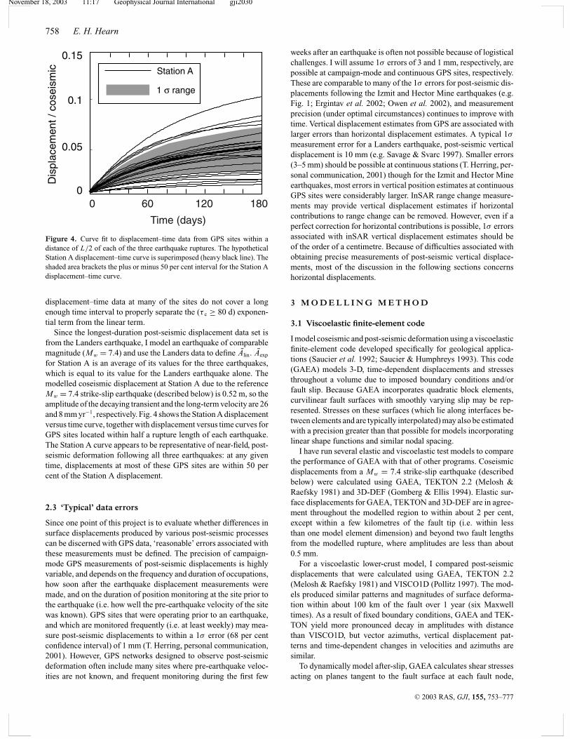
Figure 7. Station A displacements versus non-dimensionalized time for the group 1A, 1B and 1C viscoelastic models. Each curve represents a differentviscoelastic layer thickness h (as labelled). If solely Maxwell time (or, for the second column, Elsasser time) governed the time dependence of near-fieldpost-seismic deformation, only a single curve would be visible on each plot (i.e. curves for models with different values of h would be superposed).
Within model groups 1A, 1B and 1C, the evolution of surface dis-placements with time depends on both h and η, rather than just theirratio (which is proportional to T E). Fig. 7 shows modelled StationA displacements plotted against non-dimensionalized time (t/T E
and t/T M) for all of the group 1A, 1B and 1C models. If modelswith the same T E yielded similar displacement histories at StationA, curves from models with different viscoelastic layer thicknesseswould plot on top of each other. For models with small h, modelswith similar T E yield similar (though not identical) displacementswith time. For models with large h, results become increasingly sim-ilar to those predicted by layer-over-viscoelastic half-space models,for which the time dependence of deformation is characterized byT M. For most of the models shown in Fig. 7, changes to h yielddistinct displacement–time curves, regardless of how time is non-dimensionalized. This is why specific values of both h and η arespecified for models VE-1B and VE-1C.
4.1.2 Non-linear crust or mantle layer
The best non-linear lower-crust model (VE-2A) with n = 3 fits earlypost-seismic displacements at Station A reasonably well: the SSR is2.5 × 10−4, consistent with a mean misfit per 10 d epoch of 2.5 mm.The best-fitting non-linear crust model requires σ pre to be about0.02 MPa and ηpre to be about 1021 Pa s. Although this model doesnot fit the Station A displacement–time curve as well as model VE-1C, models with different plate thicknesses or values of n probablycould, although examining this possibility is not within the scope ofthis paper.
The best non-linear upper-mantle model (VE-2B) requires valuesof ηpre and σ pre to be about 1019 Pa s and 0.001 MPa, respectively.This model yielded an SSR of 0.0016 m2, comparable to that ofthe best-fitting line (0.0024 m2), and a mean misfit per 10 d epoch
of 7 mm. Thus, all of the group 2B n = 3 non-linear mantle mod-els are inconsistent with the Station A post-seismic displacementhistory. The apparent decay time for the best-fitting model is ofthe order of 10–20 d and the post-seismic velocity levels off toless than 1 mm yr−1 within weeks of the earthquake (Fig. 5). If ahigher pre-earthquake stress is modelled, the decay time for the earlypost-seismic deformation increases, but the amplitude becomes verysmall, degrading the overall fit to the Station A displacement–timecurve.
4.1.3 Velocity-strengthening frictional after-slip
For V 0 = 10 mm yr−1, the best velocity-strengthening after-slipmodel (FS) requires (a − b) = 0.001 (assuming σ ′
n = 20 MPa km−1).Incorporating layered elastic structure may double this estimate (e.g.Hearn et al. 2002) bringing it within the range of laboratory (a− b) estimates for creeping crustal shear zones (e.g. 0.001–0.01,Blanpied et al. 1995). The SSR for the best frictional after-slipmodel assuming V 0 = 10 mm yr−1 is 5.9 × 10⁻⁴ m2, consistentwith fitting the displacements every 10 d to within less than 3 mm.The sensitivity of the SSR to V 0 is low if V 0 ≥ 10 mm yr−1 (Fig. 6).
Frictional after-slip models produce very rapid velocities im-mediately after an earthquake. Since even continuous GPS cannotusually capture displacements during the first hours after an earth-quake (T. Herring, personal communication, 2001), the Station Adisplacement–time curve would not include them. Because of this,I exclude modelled displacements from the first day after the earth-quake when comparing frictional after-slip model displacements tothe Station A displacement history. Still, most of the misfit resultsfrom too rapid velocity decay immediately after the modelled earth-quake.
The uniform-slip coseismic model yields a narrow depth intervalbelow the dislocation with a high slip gradient and thus high shear
C© 2003 RAS, GJI, 155, 753–777

November 18, 2003 11:17 Geophysical Journal International gji2030
764 E. H. Hearn
stress (of the order of 10 MPa). Since real earthquakes appear to havepatchy slip distributions, it is uncertain whether local patches withhigh stress (which cause the very high initial post-seismic velocities)are present—this depends on how smooth the slip distribution is, andcurrent seismic and geodetic slip inversion techniques do not havethe resolution to answer this question. For models with a linearlytapered drop-off in slip between 10 and 15 km depth (maximumcoseismic shear stress of about 2 MPa), much smaller misfits to theStation A displacement history may be obtained (3.4 × 10⁻⁵ m2
for V 0 = 10 mm yr−1) and the (a − b) estimate is somewhat lower(3.4 × 10⁻⁵).
4.1.4 Viscous shear zone creep
Viscous shear zone models with uniform (η/w)z either (1) vastlyoverpredict the average velocity at Station A (i.e. the displacementafter 1 yr) but obtain the decay constant for the exponential termor (2) yield the correct average velocity but not the observed decayin post-seismic velocity. However, models with a step increase in(η/w)z at the mantle yield a better fit to the Station A displacementhistory. For the best viscous creep model (VC), (η/w)z declines from4.0 × 1015 Pa s m−1 (or higher) at 15 km depth down to a minimumof 1012 Pa s m−1 at 30 km depth. Assuming the shear zone is 100 mwide at a depth of 15 km, the required shear zone effective viscosityat this depth is 4.0 × 10¹⁷ Pa s. If the shear zone width is 10 km at adepth of 30 km (e.g. Hanmer 1988), model VC requires the effectiveviscosity at this depth to be 1016 Pa s. The SSR for this model is5.0 × 10−4 m2, corresponding to a mean misfit of about 4 mm tothe Station A displacement–time curve at each 10 d epoch. In thismodel, most of the early after-slip occurs at depths between 20 and33 km.
4.2 Comparison of displacement fields
Models that can reproduce early post-seismic displacements at Sta-tion A produce distinct patterns of surface deformation elsewhere. Inthis section, I highlight differences in spatial and temporal patternsof surface displacements resulting from post-seismic frictional slip,viscous creep on a vertical shear zone and relaxation of viscoelasticlayers.
4.2.1 Linear viscoelastic models: horizontal deformation
Fig. 8 shows total horizontal displacements after 180 d at 45 loca-tions within 1.5L (i.e. 100 km) of the modelled rupture. In additionto models VE-1B and VE-1C, which on average fit displacementsat Station A to within 3 mm, model VE-1A (which does not) isshown. Model VE-1A is included in Fig. 8 to illustrate how elasticlayer thickness (H) influences patterns of early post-seismic defor-mation when near-field displacements (i.e. at Station A) are con-strained to be the same. Fig. 9 shows how displacement azimuthsand amplitudes vary along three transects (11′, 22′ and 33′) shown inFig. 8.
The distance to the modelled amplitude maximum along a per-pendicular transect bisecting the fault (11′; Fig. 9) appears to beapproximately equal to H for most of the models, though this in-creases for models with thicker viscoelastic layers. For comparison,2-D analytical solutions for an elastic plate over a viscoelastic half-space (i.e. h and L = ∞) indicate that the distance to the displace-ment maximum within about two Maxwell times of the earthquakeshould be approximately 1.7H (Cohen 1999, Fig. 9). The difference
0 KM20406080100
1 1’
B
C
2 2’ 3
3’
0.5
1.0
1.5
0 F
L
D
E
F
VE_1A
VE_1B
VE_1C
Displacement at station A ( ) is 30 mm G
Figure 8. Horizontal displacements 80 d after the hypothetical Mw = 7.4strike-slip earthquake. For this plot, group 1A, 1B and 1C model parametersare chosen to yield a displacement of 30 mm at Station A 80 d after theearthquake. Amplitudes and azimuths at other locations differ significantlyfor the three models.
is likely to be due to both the finite rupture length and drag on theupper crust from elastic rebound of material below the viscoelasticlayer (see the discussion) in my models.
Once H is known, either from measuring the distance to the max-imum fault-parallel displacement or from independent information,the maximum fault-parallel displacement along a fault-normal tran-sect (i.e. 11′) approximately constrains T E or T M (for small andlarge h, respectively). In addition, h and η of the relaxing viscoelas-tic layer may estimated independently from horizontal post-seismicdisplacements, given either (1) precise displacement measurementsalong at least two transects (11′ and 33′) over a single epoch or(2) detailed, time-varying displacements at one or more judiciouslychosen site locations (see below).
The first approach to estimating η and h is to compare the maxi-mum fault-normal displacement (which occurs along strike beyondthe fault tip; i.e. along a transect of 33′) to the maximum fault-parallel displacement, over a single (early post-seismic) time epoch.The maximum fault-normal displacement is much smaller than themaximum fault-parallel displacement if h is small (Fig. 10a). Ash increases, the magnitudes of these displacements become moresimilar.
Another indicator of the η and h of the relaxing viscoelastic layeris the width of the region in which post-seismic strain is concen-trated. This is defined as the distance from the rupture, along abisecting transect, to a point where the post-seismic displacement ishalf of the maximum displacement along this transect. For a givenH , this width (w1/2) increases with h. Fig. 10(b) illustrates that thisapproach to estimating h is more diagnostic for models with largeH because as H increases, the sensitivity of w1/2 to h increases aswell.
Fig. 9 shows that early post-seismic surface velocities and dis-placements at sites along transects of 11′ and 33′ may initially beopposite in sense to coseismic displacements if h is small. Fig. 11shows such velocity reversals on plots of displacement versus time
C© 2003 RAS, GJI, 155, 753–777
November 18, 2003 11:17 Geophysical Journal International gji2030
Dynamics of post-seismic deformation 765
0
20
40
601 1’
10 km
Nor
th (
mm
)
Figure 9
1B
1A
1C
3,4
0
20
40
60
80
0
20
40
60
80
20
0
20
40
60
Hor
izon
tal
mm
Azi
mut
h d
egre
es
Ver
tical
m
m
0
10
20
303 3’
10 km
Eas
t (m
m)
1B
1C
3,41A
2 2’
10 km
1B 3,4 1A1C
1B
3,4
1A
1C
1C 1B1A,3,4
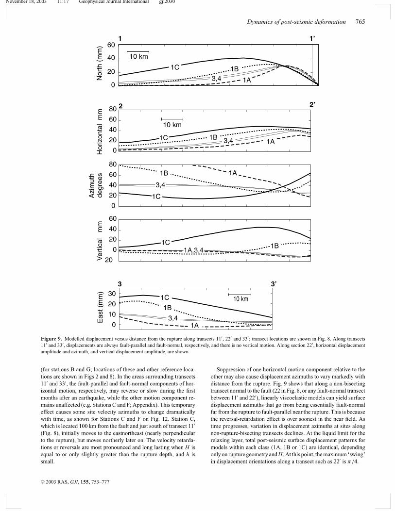
Figure 9. Modelled displacement versus distance from the rupture along transects 11′, 22′ and 33′; transect locations are shown in Fig. 8. Along transects11′ and 33′, displacements are always fault-parallel and fault-normal, respectively, and there is no vertical motion. Along section 22′, horizontal displacementamplitude and azimuth, and vertical displacement amplitude, are shown.
(for stations B and G; locations of these and other reference loca-tions are shown in Figs 2 and 8). In the areas surrounding transects11′ and 33′, the fault-parallel and fault-normal components of hor-izontal motion, respectively, may reverse or slow during the firstmonths after an earthquake, while the other motion component re-mains unaffected (e.g. Stations C and F; Appendix). This temporaryeffect causes some site velocity azimuths to change dramaticallywith time, as shown for Stations C and F on Fig. 12. Station C,which is located 100 km from the fault and just south of transect 11′
(Fig. 8), initially moves to the eastnortheast (nearly perpendicularto the rupture), but moves northerly later on. The velocity retarda-tions or reversals are most pronounced and long lasting when H isequal to or only slightly greater than the rupture depth, and h issmall.
Suppression of one horizontal motion component relative to theother may also cause displacement azimuths to vary markedly withdistance from the rupture. Fig. 9 shows that along a non-bisectingtransect normal to the fault (22 in Fig. 8, or any fault-normal transectbetween 11′ and 22′), linearly viscoelastic models can yield surfacedisplacement azimuths that go from being essentially fault-normalfar from the rupture to fault-parallel near the rupture. This is becausethe reversal-retardation effect is over soonest in the near field. Astime progresses, variation in displacement azimuths at sites alongnon-rupture-bisecting transects declines. At the liquid limit for therelaxing layer, total post-seismic surface displacement patterns formodels within each class (1A, 1B or 1C) are identical, dependingonly on rupture geometry and H . At this point, the maximum ‘swing’in displacement orientations along a transect such as 22′ is π/4.
C© 2003 RAS, GJI, 155, 753–777

November 18, 2003 11:17 Geophysical Journal International gji2030
766 E. H. Hearn
Max
imum
Fau
lt-P
aral
lel
D
ispl
acem
ent
mm
215
25125
1A0 - 0.10.1 - 0.50.5 - 1
1 - 1.51.5 - 2>2
T/TM
0
20
40
60
80
100
120
140
160
0.60.2 0.3 0.4 0.5
Max. Fault-normal / Max. Fault-Parallel
2
8
25115
1B
0
20
40
60
80
100
120
0.6 0.7 0.8 0.9 1.0
0 - 0.20.2 - 11 - 2
2 - 33 - 4>4
Max
imum
Fau
lt-P
aral
lel
D
ispl
acem
ent
mm
0102030405060708090
0.7 0.8 0.9 1
3
1752
107
1C0 - 22 - 1010 - 20
20-3030-40>40
T/TM
Max
imum
Fau
lt-P
aral
lel
D
ispl
acem
ent
mm
Half-Width of Deformed Region km
26 28 30 32 34 36 38
1A
2
15
25
30
125
0
20
40
60
80
100
120
140
160
0 - 0.10.1 - 0.50.5 - 1
1 - 1.51.5 - 2>2
T/TM
40 50 60 70 80 90 1000102030405060708090
3
17
52107
1D
0 - 22 - 1010 - 20
20-3030-40>40
T/TM
0
20
40
60
80
100
120
30 40 50 60 70 80 90
28
25
115
1B
0 - 0.20.2 - 11 - 2
2 - 33 - 4>4
T/TM
(a) (b)
Figure 10. (a) Maximum fault-parallel displacement along 11′ plotted against the ratio of maximum fault-normal displacement (along 33′) to maximumfault-parallel displacement. Linear viscoelastic model groups 1A, 1B and 1C are shown on the top, middle and bottom plots, and each curve represents adifferent value of h. Shading of symbols illustrates non-dimensionalized time. Note the difference in horizontal axis scales; the group 1A models exhibit lessfault-normal displacement beyond the rupture tip than group 1B and 1C models; this can also be seen in Fig. 8. (b) Maximum fault-parallel displacement along11′ plotted against the half-width of the deforming region, (w1/2; defined in text). For models with the smallest H (i.e. the group 1A models), early post-seismicdeformation is concentrated closest to the fault; this may also be seen in Figs 8 and 9. Note that the ratio of maximum fault-normal to maximum fault-paralleldisplacement and w1/2 are also sensitive to h.
C© 2003 RAS, GJI, 155, 753–777
November 18, 2003 11:17 Geophysical Journal International gji2030
Dynamics of post-seismic deformation 767
0 1 2 3 45
0
5
10
N m
m
125
25215
1A
0 1 2 3 4 5 6 7 8 9 105
0
5125
252
151A
0 5 10 15 20 25
0
10
20
30
N m
m
11525
82
1B
0 5 10 15 20 250
10
20
115 25
2
81B
0 4 8 12 16 200
20
4052
17107
3
N m
m 1C
0 10 20 30 40 50 60 70
20
20
0
40
60
52,17107
31C
Time / Elsasser TimeTime / Maxwell Time
E m
m
0 0.5 1 1.5 2 2.5 3 3.5 4 4.55
0
5
10
125
215, 25
1A
0 1 2 3 4 5 6 7 8 9 105
0
5
125
2515
2
1A
E m
m
0 5 10 15 20 250
10203040
11525 8
2
1B
0 5 10 15 20 250
10
20
30
11525
8,2 1B
0 2 4 6 8 10 12 14 16 18 20
0
20
40
3
10752
17
E m
m 1C
0 10 20 30 40 50 60 70-20
0
20
40
60107
31752
1C
Site B
Site G
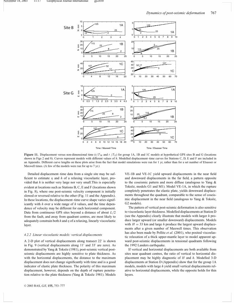
Figure 11. Displacement versus non-dimensional time (t/T M and t /T E) for group 1A, 1B and 1C models at hypothetical GPS sites B and G (locationsshown in Figs 2 and 8). Curves represent models with different values of h. Modelled displacement–time curves for Stations C, D, E and F are included inan Appendix. Different curve lengths on these plots arise from the fact that model simulations were run for 1 yr, rather than for a set number of Elsasser orMaxwell times. (A few of the models were run for up to 7 yr.)
Detailed displacement–time data from a single site may be suf-ficient to estimate η and h of a relaxing viscoelastic layer, pro-vided that h is neither very large nor very small.This is especially
evident at locations such as Stations B, C, E and F (locations shownin Fig. 8), where one post-seismic velocity component is initiallyslowed or reversed relative to the other (Fig. 11 and the Appendix).In these locations, the displacement–time curve shape varies signif-icantly with h over a wide range of h values, and the time depen-dence of velocity may be different for each horizontal component.Data from continuous GPS sites beyond a distance of about L/2from the fault, and away from quadrant centres, are most likely toadequately constrain both h and η of a relaxing, linearly viscoelasticlayer.
4.2.2 Linear viscoelastic models: vertical displacements
A 2-D plot of vertical displacements along transect 22′ is shownin Fig. 9 (vertical displacements along 11′ and 33′ are zero). Asdemonstrated by Yang & Toksoz (1981), post-seismic vertical post-seismic displacements are highly sensitive to plate thickness. Aswith the horizontal displacements, the distance to the maximumdisplacement does not change significantly with time and is a goodindicator of elastic plate thickness. The polarity of this maximumdisplacement, however, depends on the depth of rupture penetra-tion relative to the plate thickness (Yang & Toksoz 1981). Models
VE-1B and VE-1C yield upward displacements in the near fieldand downward displacements in the far field, a pattern oppositeto the coseismic pattern and more diffuse (analogous to Yang &Toksoz, models G1 and M1). Model VE-1A, in which the rupturecompletely penetrates the elastic plate, yields downward displace-ments throughout the quadrant, comparable to the sense of coseis-mic displacement in the near field (analogous to Yang & Toksoz,G2 models).
The pattern of vertical post-seismic deformation is also sensitiveto viscoelastic layer thickness. Modelled displacements at Station D(see the Appendix) clearly illustrate that models with larger h pro-duce larger upward (or smaller downward) displacements. Modelswith H = 33 km and large h produce the largest upward displace-ments after a given number of Maxwell times. This observationhas also been made by Pollitz et al. (2001), who posited viscoelas-tic relaxation of a thick upper-mantle layer to model apparent up-ward post-seismic displacements in tensional quadrants followingthe 1992 Landers earthquake.
If vertical and horizontal displacements are both available fromsites near quadrant centres, the ratio of vertical to horizontal dis-placement may be highly diagnostic of H and h. Modelled 3-Ddisplacements at Station D (Appendix) show that for the group 1Amodels, models with large h yield small vertical displacements rel-ative to horizontal displacements, while the opposite holds for thinlayers.
C© 2003 RAS, GJI, 155, 753–777
November 18, 2003 11:17 Geophysical Journal International gji2030
768 E. H. Hearn
0 10 20 30 40 50 60 70 800
5
10
15
20
25
East displacement (mm)
Nor
th d
ispl
acem
ent
(mm
)
1C
1 yr
2 yr
3 yr
9 mo3 mo
6 mo
1 yr2 yr
3 yr
9 mo
3 mo
6 mo
1 yr2 yr 3 yr
9 mo
3 mo
6 mo
4
1B
STATION F
0 5 10 155
0
5
10
15
20
25
30
35
40
East displacement (mm)
Nor
th d
ispl
acem
ent
(mm
)
1B4
3 mo
6 mo
9 mo
1 yr2 yr3 yr
3 yr6 mo
3 mo 6 mo9 mo
1 yr
2 yr
3 yr
STATION C
1C
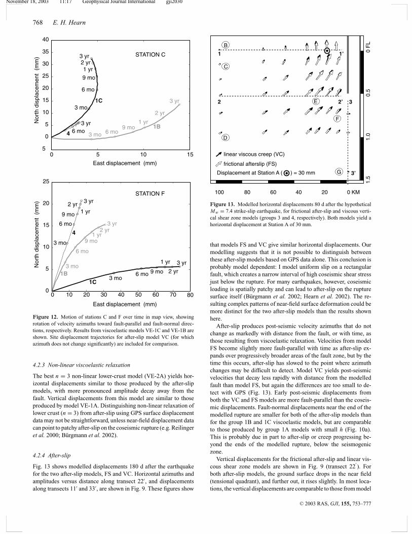
Figure 12. Motion of stations C and F over time in map view, showingrotation of velocity azimuths toward fault-parallel and fault-normal direc-tions, respectively. Results from viscoelastic models VE-1C and VE-1B areshown. Site displacement trajectories for after-slip model VC (for whichazimuth does not change significantly) are included for comparison.
4.2.3 Non-linear viscoelastic relaxation
The best n = 3 non-linear lower-crust model (VE-2A) yields hor-izontal displacements similar to those produced by the after-slipmodels, with more pronounced amplitude decay away from thefault. Vertical displacements from this model are similar to thoseproduced by model VE-1A. Distinguishing non-linear relaxation oflower crust (n = 3) from after-slip using GPS surface displacementdata may not be straightforward, unless near-field displacement datacan point to patchy after-slip on the coseismic rupture (e.g. Reilingeret al. 2000; Burgmann et al. 2002).
4.2.4 After-slip
Fig. 13 shows modelled displacements 180 d after the earthquakefor the two after-slip models, FS and VC. Horizontal azimuths andamplitudes versus distance along transect 22′, and displacementsalong transects 11′ and 33′, are shown in Fig. 9. These figures show
0 KM20406080100
1 1’
2 2’ 3
3’
0.5
1.0
1.5
0 F
LB
C
D
E
F
linear viscous creep (VC)
frictional afterslip (FS)
Displacement at Station A ( ) = 30 mm G
Figure 13. Modelled horizontal displacements 80 d after the hypotheticalMw = 7.4 strike-slip earthquake, for frictional after-slip and viscous verti-cal shear zone models (groups 3 and 4, respectively). Both models yield ahorizontal displacement at Station A of 30 mm.
that models FS and VC give similar horizontal displacements. Ourmodelling suggests that it is not possible to distinguish betweenthese after-slip models based on GPS data alone. This conclusion isprobably model dependent: I model uniform slip on a rectangularfault, which creates a narrow interval of high coseismic shear stressjust below the rupture. For many earthquakes, however, coseismicloading is spatially patchy and can lead to after-slip on the rupturesurface itself (Burgmann et al. 2002; Hearn et al. 2002). The re-sulting complex patterns of near-field surface deformation could bemore distinct for the two after-slip models than the results shownhere.
After-slip produces post-seismic velocity azimuths that do notchange as markedly with distance from the fault, or with time, asthose resulting from viscoelastic relaxation. Velocities from modelFS become slightly more fault-parallel with time as after-slip ex-pands over progressively broader areas of the fault zone, but by thetime this occurs, after-slip has slowed to the point where azimuthchanges may be difficult to detect. Model VC yields post-seismicvelocities that decay less rapidly with distance from the modelledfault than model FS, but again the differences are too small to de-tect with GPS (Fig. 13). Early post-seismic displacements fromboth the VC and FS models are more fault-parallel than the coseis-mic displacements. Fault-normal displacements near the end of themodelled rupture are smaller for both of the after-slip models thanfor the group 1B and 1C viscoelastic models, but are comparableto those produced by group 1A models with small h (Fig. 10a).This is probably due in part to after-slip or creep progressing be-yond the ends of the modelled rupture, below the seismogeniczone.
Vertical displacements for the frictional after-slip and linear vis-cous shear zone models are shown in Fig. 9 (transect 22
′). For
both after-slip models, the ground surface drops in the near field(tensional quadrant), and further out, it rises slightly. In most loca-tions, the vertical displacements are comparable to those from model
C© 2003 RAS, GJI, 155, 753–777

November 18, 2003 11:17 Geophysical Journal International gji2030
Dynamics of post-seismic deformation 769
VE-1A. However, both after-slip models yield much larger down-ward displacements immediately adjacent to the fault (between tran-sects 11′ and 22′ in Fig. 8) than model VE-1A.
5 D I S C U S S I O N
5.1 Effect of h on stress and velocity field evolution
After-slip causes the lithosphere to move horizontally in the samedirection it did during the earthquake, but viscoelastic relaxationdoes not. If a low-viscosity layer is present at some depth inthe lithosphere, only the plate above this layer deforms post-seismically in the same sense as the earthquake. As the relaxinglayer loosens its grip on the top surface of the elastic volume be-low it, this volume deforms in a sense opposite to coseismic as itrebounds to its pre-earthquake configuration (Fig. 14). To state thisin terms of the ‘jelly sandwich’ lithosphere rheology model, theslice of bread below the jelly is not fixed throughout the earthquakecycle.
As the elastic volume below the viscoelastic layer deforms, it ex-erts drag (through the viscoelastic layer) on the upper crust, whichopposes continued elastic deformation of the upper crust in the co-seismic sense. This drag may cause retardation or reversal of one orboth horizontal surface velocity components. Fault-parallel motionof the crust is slowed or reversed along transect 11′, and motionnormal to the fault is reversed or retarded along 33′ (e.g. motion ofstations B, E, F and G, Fig. 11, and Appendix). This leads to the dis-tinct spatial and temporal character of surface deformation resultingfrom viscoelastic relaxation of layers with different thicknesses butidentical Elsasser times. The drag may also explain why the dis-tance to the maximum post-seismic displacement along transect 11′
0 50 100 150 25
20
15
10
5
0
0 10 20 30 40 120
100
80
60
40
0 -.02 -.04 -.06 -.08 25
20
15
10
5
0
0 -.01 -.02 -.03 -.04 120
100
80
60
40
Dep
th k
mD
epth
km
East displacement mm Pressure MPa
a
b
c
d
cose
is
cose
is
cose
is
cose
is
7
14
714
7
14
714
Figure 14. (a) and (b) Eastward displacement of lithosphere profiles below Station E, above and below a decoupling viscoelastic layer, for model VE-1B.Coseismic displacements, as well as displacements after 7 and 14 Maxwell times, are shown. The elastic intervals above and below the viscoelastic layer movein opposite directions as horizontal shear tractions in the decoupling layer decline over time. (c) and (d) Pressure ((σ 1 + σ 2 + σ 3)/3) as a function of depthat the same location. Coseismic deformation in tensional (pressure drops) at all depths. Post-seismically (at t = 7 T M and 14T M), pressure continues to dropabove the decoupling horizon, but rises in the elastic material below it. This indicates a reversed sense of deformation on either side of the relaxing layer.
is less than predicted by the analytical solution (Cohen 1999), inwhich an infinitely thick viscoelastic layer is assumed. Since thedistinct deformation patterns for different values of h do not resultfrom end effects, they will also be evident for longer ruptures. Asshear stresses in the relaxing viscoelastic layer continue to decline,horizontal surface displacements approach patterns and amplitudesthat depend solely on H and the rupture geometry.
Vertical displacements due to post-seismic viscoelastic relaxationare affected by both the elastic upper plate thickness and the thick-ness of the relaxing layer (e.g. Yang & Toksoz 1981; Pollitz et al.2001). At a particular surface location, the vertical displacementover a post-seismic time interval is the sum of vertical strains in-tegrated over H , h and the (essentially elastic) material below. If his large, the second two terms are small. The elastic material belowa thick, relaxing viscoelastic layer contributes little to the verticaldisplacements because it is located at a great depth and underwentlittle coseismic strain. Furthermore, if two models produce com-parable, early post-seismic surface deformation in the near field,the model with large h has the lower Maxwell time and is closerto its liquid limit at any time. Thus, both volumetric strain withinthe relaxing layer and contributions to surface displacements fromintegrated vertical strain below the relaxing layer are minimized.This leaves elastic deformation of the upper plate in response to re-duced shear tractions at its base as the dominant term contributing topost-seismic surface deformation. As the substrate nears its liquidlimit, vertical surface displacements tend to be opposite in sense tocoseismic displacements (in the near field).
On the other hand, if h is small (i.e. the ‘jelly sandwich’ crustalmodel), elastic deformation of material below the relaxing layer maycontribute significantly to vertical displacements at the surface, par-ticularly in the far field. Since deformation below the viscoelastic
C© 2003 RAS, GJI, 155, 753–777

November 18, 2003 11:17 Geophysical Journal International gji2030
770 E. H. Hearn
layer is opposite in sense to the coseismic deformation, the senseof vertical strain at depth may be reversed relative to layer-over-viscoelastic-half-space models at the same time, and vertical dis-placements at the surface may also be reversed. However, since thesign of vertical strain in a volume depends on the relative mag-nitudes of the vertical and horizontal normal stresses, numericalcalculations are required to predict vertical displacements for ‘jellysandwich’ models.
Flow within the viscoelastic layer, driven by pressure gradientsbetween compressed and dilated quadrants, could provide an al-ternate explanation for early post-seismic reversals in the sense ofvertical motion (relative to coseismic displacements). Such flowwould cause pressure changes of the same sign both above and be-low the relaxing layer. Examination of model VE-1B stresses showsthat opposite signs of post-seismic pressure change occur above andbelow the relaxing layer (Fig. 14), except in the extreme near field.This shows that elastic rebound of the material below the viscoelas-tic layer is responsible for temporary post-seismic reversals of bothvertical and horizontal surface velocity components.
5.2 How geologically reasonable are the mostsuccessful models?
In the results section, non-linear relaxation of upper mantle withn = 3 (group 2B models) and linear viscoelastic relaxation ofthe lower crust immediately below the seismogenic zone (group1A models) were ruled out as possible causes for typical, earlypost-seismic deformation associated with large strike-slip earth-quakes. The remaining models (viscous and frictional after-slip,viscoelastic lower crust and linearly viscous upper mantle) repro-duce the Station A displacement–time curve with varying degreesof success. These models must also be judged on how consistenttheir required rheological parameters are with typical continentallithosphere.
5.2.1 Viscoelastic models
Model VE-1B represents linear viscoelastic relaxation of a very thinlower crustal layer or detachment, at about 25 km depth. Labora-tory experiments suggest that wet quartz (Jaoul et al. 1984; Wanget al. 1994), and wet Westerly granite (Hansen & Carter 1983) coulddeform at the viscosity required by model VE-1B at temperaturestypical for hot continental lower crust (i.e. 450–600 ◦C). However,free quartz is not present in typical lower crustal rocks (Rutter &Brodie 1992; Rudnick & Fountain 1995). Without free quartz (ormuscovite), low viscosities could still result from shear localization,which can form thin horizons with fine grain sizes and high concen-trations of volatiles, or from trapped melt along grain boundaries(Rushmer 2001). Furthermore, geophysical studies (e.g. Park et al.1992; Brocher et al. 1994; Bokelmann & Beroza 2000) and modelsof topographic collapse (Kaufman & Royden 1994; Clark & Royden2000) indicate the presence of detachments or low-viscosity crustallayers in some regions. Thus, model VE-1B could be geologicallyreasonable for some continental crust, particularly in regions withelevated geotherms.
Model VE-1C represents viscoelastic relaxation of either the bot-tom few kilometres of a thick continental crust (e.g. a model withh = 3 km) or a low-viscosity interval in the uppermost mantle, pre-sumably under atypically strong crust (similar to the model of Pollitzet al. 2001). The relaxing material could be nearly linearly viscoelas-tic (e.g. a wet quartz rheology), or a non-linear material under sucha large differential stress that the coseismic stress change has a neg-ligible effect on the effective viscosity (see eq. 6) and its response to
the earthquake appears to be identical to that of a linearly viscoelas-tic material. Assuming a wet olivine flow law (Karato & Wu 1993;Mei & Kohlstedt 2000) and high temperatures and/or differentialstresses in the upper mantle, effective viscosity values required byour models (e.g. of the order of 1017 Pa s) can be obtained, butnot under geologically tenable conditions. If the upper mantle is at1100 ◦C (1400 ◦K), a differential stress of 100 MPa is needed toattain the required model viscosity of 1017 Pa s, and mantle strainrates must be of the order of 10−9 s−1. For more typical upper-mantletemperatures, the required differential stress and strain rate are evengreater. For comparison, mantle stresses have been estimated frompaleopeizometric studies of xenoliths and ophiolites at 1–100 MPa,and strain rates of 10−12–10−17 s−1 have been inferred from studiesof olivine grain size in the upper mantle (see the summary by Carter& Tsenn 1987). The temperature and stress requirements of olivineflow laws appear to rule out mantle relaxation as a likely cause forrapid post-seismic deformation anywhere, unless a significant per-centage of melt is present (e.g. Kohlstedt et al. 1995). It is difficult topicture why a relatively thin (17 km thick) mantle layer immediatelybelow the crust would be significantly weaker than the surroundinglithosphere.
Model VE-1C may also represent post-seismic relaxation ofquartzofeldspathic lower crust in areas with high crustal thickness.The effective viscosity required by model VE-1C (1017 Pa s) is con-sistent with a quartz-controlled (linear) rheology in hot lower crust(i.e. 500–600 ◦C), and may be geologically reasonable in some re-gions. However, non-linear flow laws for more typical lower crustalrocks (in which feldspar is the rate-controlling component) do notyield the required effective viscosity at stresses of less than about100 MPa (e.g. Shelton & Tullis 1981; Caristan 1982). For such alow-viscosity material to maintain differential stresses of 100 MPa,the strain rate would have to be unreasonably high for the lower crust(10−9 s−1).
Non-linear lower-crust model VE-2A reproduces the referencedisplacements at Station A reasonably well, given ηpre of the orderof 1021 Pa s and σ pre of the order of 2 to 5 × 10⁴ Pa (implying avery low strain rate in the lower crust). As Fig. 6 illustrates, theseparameters must be finely tuned. Immediately after the earthquake,when the differential stress increases by a few MPa in the near field,the effective viscosity of the lower crust in that area must declineto 1017 Pa s. Non-linear flow laws for feldspathic rocks suggestthat at 500–600 ◦C, differential stresses of the order of 100 MPaare required to obtain ηeff ≈ 1017 Pa s. This vastly exceeds themaximum coseismic stress change in the lower crust, so coseismicweakening of non-linearly viscoelastic lower crust (with n ≈ 3) isprobably not responsible for rapidly decaying, early post-seismicdeformation. However, a suite of non-linear models with n between1 and 3 and H between 15 and 25 km could be devised to reproduceearly post-seismic displacements at Station A. Values of ηpre andσ pre for some of these models could be compatible with known flowlaws for crustal rocks.
5.2.2 After-slip models
The frictional after-slip model FS requires a value of velocity-strengthening parameter (a − b) that is at the bottom of the rangefor velocity-strengthening crust below the seismogenic zone. Low(a − b) values have been estimated from an analysis of post-seismicdata from both the Loma Prieta, California and Izmit, Turkey earth-quakes (e.g. Linker & Rice 1997; Hearn et al. 2002). One interpre-tation is that the product (a − b)σ ′
n is low because σ ′n is small. This
could happen if pore pressures in the fault zone were high enough to
C© 2003 RAS, GJI, 155, 753–777
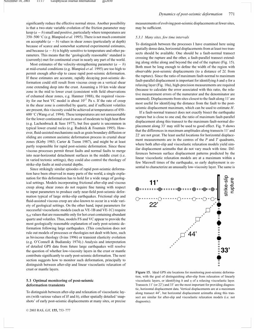
November 18, 2003 11:17 Geophysical Journal International gji2030
Dynamics of post-seismic deformation 771
significantly reduce the effective normal stress. Another possibilityis that a two-state variable evolution of the friction parameter maykeep (a − b) small and positive, particularly where temperatures are350–500 ◦C (e.g. Blanpied et al. 1995). There is not much constrainton acceptable (a − b) values in shear zones (particularly at depth)because of scarce and somewhat scattered experimental estimates,and because (a − b) is highly sensitive to temperature and other pa-rameters. This means that the ‘geologically reasonable’ standard is(currently) met for continental crust in nearly any part of the world.
Most estimates of the velocity-strengthening parameter (a − b)at mid-crustal conditions (e.g. Blanpied et al. 1995) are too high topermit enough after-slip to cause rapid post-seismic deformation.If these estimates are accurate, rapidly decaying post-seismic de-formation could still result from viscous creep on a vertical shearzone extending deep into the crust. Assuming a 10 km wide shearzone in the mid to lower crust (consistent with field observationsof exhumed shear zones, e.g. Hanmer 1988), the required viscos-ity for our best VC model is about 1017 Pa s. If the rate of creepin the shear zone is controlled by quartz, and if sufficient volatilesare present, this viscosity could be achieved at temperatures of 450–600 ◦C (Wang et al. 1994). These temperatures are not unreasonablefor the lower continental crust in areas of moderate to high heat flow(e.g. Lachenbruck & Sass 1977), but free quartz is uncommon intypical lower crustal rocks (e.g. Rudnick & Fountain 1995). How-ever, fluid-assisted mechanisms such as grain boundary diffusion orsliding are common aseismic deformation process in crustal shearzones (Kirby 1983; Carter & Tsenn 1987), and might be at leastpartly responsible for rapid post-seismic deformation. Since theseviscous processes permit thrust faults and normal faults to mergeinto near-horizontal detachment surfaces in the middle crust (i.e.in varied tectonic settings), they could also control the rheology ofstrike-slip faults at mid-crustal depths.
Since strikingly similar episodes of rapid post-seismic deforma-tion have been observed in many parts of the world, a single expla-nation for this deformation has to hold for a wide range of geolog-ical settings. Models incorporating frictional after-slip and viscouscreep along shear zones do not require fine tuning with respectto input parameters to produce early near-field post-seismic defor-mation typical of large strike-slip earthquakes. Frictional slip andfluid-assisted viscous creep are also known to occur in a wide vari-ety of geological settings. On the other hand, input parameters forsuccessful viscoelastic models (such as VE-1B and VE-1C) requireηeff values that are reasonable only for hot crust containing abundantquartz and volatiles. Thus, models FS and VC appear to provide themost geologically reasonable explanation of early post-seismic de-formation following large earthquakes. (This conclusion does notrule out models of processes or rheologies not dealt with here, suchas biviscous rheology (Ivins 1996) or transient elasticity evolution(e.g. O’Connell & Budiansky 1974).) Analysis and interpretationof detailed GPS data from future large earthquakes will resolvethe question of whether low-viscosity layers in the crust or mantlecontribute significantly to early post-seismic deformation. The nextsection suggests how to monitor such deformation, principally todistinguish between after-slip and linear viscoelastic relaxation ofcrust or mantle layers.
5.3 Optimal monitoring of post-seismicdeformation transients
To distinguish between after-slip and relaxation of viscoelastic lay-ers (with various values of H and h), either spatially detailed ‘snap-shots’ of early post-seismic displacements at many sites, or precise
measurements of evolving post-seismic displacements at fewer sites,may be sufficient.
5.3.1 Many sites, few time intervals
To distinguish between the processes I have examined here usingspatially dense data, horizontal displacements from at least two tran-sects should be available. One should be a fault-normal transectcrossing the rupture and the other, a fault-parallel transect extend-ing along strike along and beyond the end of the rupture (Fig. 15).Both must be long enough to define the width of the region withobservable post-seismic displacements (to a distance of 2L fromthe rupture). Since the ratio of maximum fault-normal to maximumfault-parallel displacement is important for identifying h and η for arelaxing layer (Fig. 10a), high-precision measurements are required(because to calculate the error associated with this ratio, the rela-tive measurement errors of the numerator and the denominator aresummed). Displacements from sites closest to the fault along 11′ aremost useful for identifying the distance from the fault to the post-seismic displacement maximum, which can be used to estimate H .
If a fault-normal transect does not exactly bisect the earthquakerupture but is close to one end, the ratio of maximum fault-paralleldisplacement along this transect to the maximum fault-normal dis-placement along 33′ may still be used to good effect. Fig. 9 showsthat the differences in maximum amplitudes along transects 11′ and22′ are not great. The least useful locations for horizontal displace-ment measurements are in the centres of the P and T quadrants,where both after-slip and viscoelastic relaxation models yield sim-ilar displacement azimuths that do not vary much with time. Dif-ferences between surface displacement patterns predicted by thelinear viscoelastic relaxation models are at a maximum within afew Maxwell times of the earthquake, so early deployment is es-sential to characterize an unusually low-viscosity layer. The same is
11’
22’
33’
44’ s
trik
e-sl
ip
rup
ture
Figure 15. Ideal GPS site locations for monitoring post-seismic deforma-tion, with the goal of distinguishing after-slip from relaxation of linearlyviscoelastic layers, or identifying h and η of a relaxing viscoelastic layer.Transects 11′ (or 22′) and 33′ are the most important for providing diagnos-tic, horizontal displacement data. Vertical displacements are at a maximumalong transect 44′′, but horizontal displacement azimuths along this tran-sect are similar for after-slip and viscoelastic relaxation models (i.e. notdiagnostic).
C© 2003 RAS, GJI, 155, 753–777

November 18, 2003 11:17 Geophysical Journal International gji2030
772 E. H. Hearn
true for characterizing after-slip, which may decay rapidly after anearthquake (e.g. Tse & Rice 1986; Marone et al. 1991; Burgmannet al. 2002; Hearn et al. 2002). In general, measurement precisionis important, so GPS sites where pre-earthquake velocities are wellquantified (and hence where errors to corrections for secular de-formation are small) should be monitored frequently, even if theirlocations are not ideal.
In contrast to horizontal displacements, the maximum differencesbetween modelled vertical displacements occur at the centres of Pand T quadrants. A transect of continuous GPS stations extend-ing diagonally outward from the rupture tip could define verticaldisplacement as a function of distance to the fault. (InSAR interfer-ograms, on the other hand, are a poor proxy for a map of verticaldisplacements because for strike-slip earthquakes, range changesreflect mostly horizontal motion.) The interpretation of vertical dis-placements is complicated by the fact that the sign of these dis-placements (up or down) changes with time at different rates inmost areas (except the near field, where poroelastic deformationand irregularities in slip distribution may make interpretation chal-lenging anyway). Shallow viscoelastic relaxation and after-slip alsoyield similar vertical displacements (Fig. 9). Given typical mea-surement errors for vertical displacements, it is unlikely that oneof the aseismic deformation scenarios presented here could be dis-tinguished from the others based solely on vertical displacements,except for linear relaxation of the mantle (see Fig. 9, transect 22′).Vertical and horizontal displacements together may be diagnostic,particularly for identifying viscoelastic relaxation of lower crust orupper-mantle layers, but interpretation of such data requires detailednumerical modelling because of the extreme sensitivity of verticaldisplacements to small changes in h, H , rupture depth and location.
5.3.2 Temporally detailed data from a few GPS sites
Detailed measurements of time-varying velocities at a few GPSsites may provide enough information to at least rule out severalcandidate models. Data from sites in the intermediate to far fieldalong transects 33′ and 11′ (or 22′) are the most useful for discerningbetween viscoelastic relaxation models. The principal rule is, avoidthe centres of P and T quadrants.
Time-dependent displacement data from GPS sites at P–T quad-rant centres or adjacent to the fault may provide only limited con-straints for viscoelastic models because several non-unique combi-nations of h and η may adequately explain displacement–time curvesat those locations. At most sites along transect 22′, and in other ar-eas not close to quadrant centres, one of the horizontal components(fault-parallel or fault-normal) is initially slowed or reversed. Thisleads to velocity azimuth rotation with time (Fig. 12), which may bemodelled to estimate both h and η. In general, velocity azimuths atsites along strike (or in that vicinity, e.g. Stations E and F) becomeincreasingly fault-normal with time if viscoelastic layer relaxationis occurring, and velocities of sites just off the bisecting transect(e.g. Station C) gradually become more fault parallel. Since after-slip yields fault-parallel and fault-normal velocity components witha similar time dependence, decaying post-seismic velocities withunchanging azimuths at sites positioned like Stations C, E and Findicate after-slip. If continuous GPS data are available from sitesat different distances from the rupture, comparing apparent τ c isinstructive: increases to tauc with distance from the rupture signalviscoelastic relaxation rather than after-slip. Also, if spatially de-tailed displacement data show strain concentrated around the ruptureand appear consistent with either after-slip or viscoelastic relaxationwith H ≈ 15 km, continuous GPS data may prove decisive. In this
case, rapidly decaying surface velocities (τ c ≈ 80 d) would indicateafter-slip and near-constant velocities would indicate viscoelasticrelaxation.
5.3.3 Real earthquakes
Each earthquake presents its own set of logistical challenges forGPS monitoring, and measuring time-dependent post-seismic dis-placements in the areas shown in Fig. 15 (and near pre-existing GPSsites where secular velocity corrections can be made) may be im-possible. In addition, ideal monitoring strategies depend on whichphenomenon is to be characterized (which is unknown beforehand).Characterizing relaxing viscoelastic relaxation lower crust or man-tle layers, or telling after-slip from viscoelastic relaxation, has beenthe focus of the previous section, and recommendations for moni-toring post-seismic deformation with this in mind were given above.However, if the focus is on the dynamics of after-slip (e.g. Hearnet al. 2002) then GPS sites are close to the rupture, where they maynot provide much useful information on anything else.
To some extent, the questions that can be adequately answeredfrom modelling post-seismic deformation may be serendipitous, de-pending on where GPS displacement measurements can be made af-ter a particular earthquake. However, since one contentious questionamong earthquake scientists is whether or not significant relaxationof the upper mantle is redistributing stresses over large areas dur-ing the years following large earthquakes, efforts should be madeto design post-seismic GPS networks to answer this question. Todo so, the network must include several sites along strike beyondthe rupture tip (not just along transects crossing the rupture), andfrequent (or continuous) monitoring of distant sites is as importantas (or more important than) frequent monitoring of sites near therupture.
6 C O N C L U S I O N S
Several after-slip and viscoelastic relaxation models adequately re-produce early, near-field post-seismic displacements typical of largestrike-slip earthquakes, including their time dependence (i.e. veloc-ity decay). However, modelled displacements away from the ref-erence point are distinct and may evolve with time, particularlyfor models incorporating relaxation of linearly viscoelastic layers.GPS data from either continuous or frequently monitored campaign-mode sites in well-chosen locations may be sufficient to resolve thecause of post-seismic deformation (i.e. after-slip versus relaxationof linearly viscoelastic layers), and, for a relaxing Newtonian layer,to resolve both its viscosity and its thickness.
GPS sites should not be concentrated adjacent to the rupture ifthe object of monitoring is to identify possible relaxation of linearlyviscoelastic mantle or lower crust. In this case, the best locations forGPS sites are along fault-parallel transects extending at least onefault length beyond the ends of the rupture (transect 33′ in Fig. 15),and along another transect crossing the rupture (transects 11′ and22′ in Fig. 15).
The ‘smoking gun’ for relaxation of linearly viscoelastic layersat depth (i.e. H = 25+ km) is a large component of fault-normalmotion at sites beyond the rupture tip. (A broad region of high strain(w1/2) and uplift of extensional quadrants in the near field are also di-agnostic.) Post-seismic velocity azimuths that change dramaticallyover time (due to differences in time dependence of the fault-normaland fault-parallel velocity components) indicate relaxation of a thin,linearly viscoelastic layer or horizontal shear zone. If GPS site ve-locity azimuths do not change with time, and if horizontal velocitiesdecay at a comparable rate at all distances from the rupture, then
C© 2003 RAS, GJI, 155, 753–777
November 18, 2003 11:17 Geophysical Journal International gji2030
Dynamics of post-seismic deformation 773
of the processes modelled here, after-slip (or perhaps relaxation ofnon-linear material in the mid to lower crust) is most likely. Smallfault-normal displacements near and beyond the fault tip also sug-gest that relaxation of linearly viscoelastic layers at depth below therupture is not occurring.
Two classes of models I developed for this study could not producetime-dependent near-field displacements typical of large strike-slipearthquakes: linearly viscoelastic models with H = 15 km (group1A) and non-linearly viscoelastic models with n = 3 and H =33 km (group 2B). Though the target displacement–time curve isnot too well constrained (Fig. 4), data from the three earthquakesstill require a decaying transient with a characteristic time of theorder of 80 d, and a total displacement after 1 yr of the order of tensof millimetres. Models from groups 1A and 2B cannot meet bothrequirements. Furthermore, the ηeff value required by model VE-1Crequires a geologically unreasonable strain rate of the order of 10−9
s−1 in the upper mantle (assuming a hot upper mantle and a wetperidotite flow law). This suggests that rapid viscoelastic relaxationis more likely to occur in the lower crust rather than in the uppermantle.
A C K N O W L E D G M E N T S
This research was supported by the Southern California EarthquakeCenter. SCEC is funded by NSF Cooperative Agreement EAR-0106924 and USGS Cooperative Agreement 02HQAG0008. TheSCEC contribution number for this paper is 716. I would like tothank Fred Pollitz and Shoichi Yoshioka for their comments onthe manuscript. I would also like to thank Brad Hager and RolandBurgmann for their suggestions on earlier drafts of this paper.
R E F E R E N C E S
Blanpied, M.L., Lockner, D.A. & Byerlee, J.D., 1995. Frictional slip ofgranite at hydrothermal conditions, J. geophys. Res., 100, 13 045–13 064.
Bock, Y. et al., 1997. Southern California Permanent GPS Array: continuousmeasurements of regional crustal deformation between the 1992 Landersand 1994 Northridge Earthquakes, J. geophys. Res., 102, 18 013–18 033.
Bokelmann, G. & Beroza, G., 2000. Depth-dependent earthquake focalmechanism orientations: evidence for a weak zone in the lower crust,J. geophys. Res., 105, 21 683–21 695.
Brocher, T.M., McCarthy, J., Hart, P.E., Holbrook, W.S. & Furlong, K.P.,1994. Seismic evidence for a lower crustal detachment beneath San Fran-cisco Bay, California, Science, 265, 1436–1439.
Burgmann, R., Ergintav, S., Segall, P., Hearn, E.H., McClusky, S., Reilinger,R.E., Woith, H. & Zschau, J., 2002. Time–space variable afterslip on anddeep below the Izmit earthquake rupture, Bull. seism. Soc. Am., 92, 126–137.
Caristan, Y., 1982. The transition from high-temperature creep to fracture inMaryland Diabase, J. geophys. Res., 87, 6781–6790.
Carter, N.L. & Tsenn, M.C., 1987. Flow properties of continental litho-sphere, Tectonophysics, 136, 27–63.
Clark, M.K. & Royden, L.H., 2000. Topographic ooze: building the easternmargin of Tibet by lower crustal flow, Geology, 28, 703–706.
Cohen, S.C., 1999. Numerical models of crustal deformation in seismiczones, Adv. Geophys., 41, 133–231.
Deng, J., Gurnis, M., Kanamori, H. & Hauksson, E., 1998. Viscoelastic flowin the lower crust after the 1992 Landers, California earthquake, Science,282, 1689–1692.
Dieterich, J.H., 1979. Modeling of rock friction 1. Experimental results andconstitutive equations, J. geophys. Res., 84, 2161–2168.
Ergintav, S., Burgmann, R., McClusky, S., Cakmak, R., Reilinger, R.E.,Lenk, O., Barka, A. & Gurkan, O., 2002. Postseismic deformation nearthe Izmit earthquake 17 August, 1999, Bull. seism. Soc. Am., 92, 194–207.
Freed, A.M. & Lin, J., 2001. Delayed triggering of the 1999 Hector Mineearthquake by viscoelastic stress transfer, Nature, 411, 180–183.
Gomberg, J. & Ellis, M., 1994. Topography and tectonics of the central NewMadrid seismic zone: results of numerical experiments using a three-dimensional boundary-element program, J. geophys. Res., 99, 20 299–20 310.
Hanmer, S., 1988. Great Slave Lake shear zone, Canadian Shield: recon-structed vertical profile of a crustal scale fault zone, Tectonophysics, 149,245–264.
Hansen, F.D. & Carter, N.L., 1983. Semibrittle creep of dry and wet WesterlyGranite at 1000 MPa, 24th US Symp. on Rock Mechanics, Texas A&MUniversity, College Station, TX.
Hearn, E.H., Burgmann, R. & Reilinger, R., 2002. Dynamics of Izmit earth-quake postseismic deformation and loading of the Duzce earthquakehypocenter, Bull. seism. Soc. Am., 92, 172–193.
Heki, K.S., Miyazaki, S. & Tsuji, H., 1997. Silent slip following an interplatethrust earthquake at the Japan Trench, Nature, 386, 595–598.
Hsu, Y.-J., Bechor, N., Segall, P., Yu, S.-B. & Ma, K.-F., 2002. Rapid afterslipfollowing the 1999 Chi-Chi, Taiwan earthquake, Geophys. Res. Lett., 29,10.1029/2002GL014967.
Ivins, E.R., 1996. Transient creep of a composite lower crust, 2. A polymin-erallic basis for rapidly evolving postseismic deformation modes, J. geo-phys. Res., 101, 28 005–28 028.
Jaoul, O., Tullis, T. & Kronenburg, A., 1984. The effect of varying watercontents on the creep behaviour of Heavitree quartzite, J. geophys. Res.,89, 4298–4312.
Karato, S.-I. & Wu, P., 1993. Rheology of the upper mantle: a synthesis,Science, 260, 771–778.
Kaufman, P.S. & Royden, L.H., 1994. Lower crustal flow in an extensionalsetting: constraints from the Halloran Hills region, eastern Mojave Desert,J. geophys. Res., 99, 15 723–15 739.
Kenner, S.J. & Segall, P., 2000. Postseismic deformation following the 1906San Francisco earthquake, J. geophys. Res., 105, 13 195–13 209.
Kirby, S.H., 1983. Rheology of the lithosphere, Rev. Geophys. Space Phys.,21, 1458–1487.
Kohlstedt, D.L., Evans, B. & Mackwell, S.J., 1995. Strength of the litho-sphere: constraints imposed by laboratory experiments, J. geophys. Res.,100, 17 587–17 602.
Lachenbruck, A.H. & Sass, J.H., 1977. Heat flow in the United States andthe thermal regime of the crust, Geophys. Monograph, 20, 626–675.
Lehner, F.K., Li, V.C. & Rice, J.R., 1981. Stress diffusion along plate bound-aries, J. geophys. Res., 86, 6155–6169.
Linker, M.F. & Rice, J.R., 1997. Models of postseismic deformation andstress transfer associated with the Loma Prieta earthquake, in US Geolog-ical Survey Professional Paper 1550-D: the Loma Prieta Earthquake ofOctober 17, 1989; aftershocks and postseismic effects, pp. D253–D275.
McClusky, S. et al., 2000. Global Positioning System constraints on platekinematics and dynamics in the Eastern Mediterranean and Caucasus, J.geophys. Res., 105, 5695–5719.
McClusky, S.C., Bjornstad, S.C., Hager, B.H., King, R.W., Meade, B.J.,Miller, M.M., Monastero, F.C. & Souter, B.J., 2001. Present day kinemat-ics of the Eastern California Shear Zone from a geodetically constrainedblock model, Geophys. Res. Lett., 28, 3369–3372.
Marone, C.J., Scholz, C.H. & Bilham, R., 1991. On the mechanics of earth-quake afterslip, J. geophys. Res., 96, 8441–8452.
Meade, B., Hager, B., McClusky, S., Reilinger, R.E., Ergintav, S., Lenk, O.,Barka, A. & Ozener, H., 2002. Estimates of seismic potential in the Mar-mara Sea region from block models of secular deformation constrainedby GPS measurements, Bull. seism. Soc. Am., 92, 208–215.
Mei, S. & Kohlstedt, D.L., 2000. Influence of water on plastic deformationof olivine aggregates 2. Dislocation creep regime, J. geophys. Res., 105,21 471–21 481.
Melosh, H.J. & Raefsky, A., 1981. A simple and efficient method for intro-ducing faults into finite element computations, Bull. seism. Soc. Am., 71,1391–1400.
Nur, A. & Mavko, G., 1974. Postseismic viscoelastic rebound, Science, 183,204–206.
C© 2003 RAS, GJI, 155, 753–777

November 18, 2003 11:17 Geophysical Journal International gji2030
774 E. H. Hearn
O’Connell, R.J. & Budiansky, B., 1974. Seismic velocities in dry and satu-rated cracked solids, J. geophys. Res., 79, 5412–5426.
Owen, S. et al., 2002. Early postseismic deformation from the Mw = 7.1Hector Mine, California, earthquake as measured by survey mode GPS,Bull. seism. Soc. Am., 92, 1423–1432.
Park, S.K., Kinn, C.L. & Jiracek, G.R., 1992. Magnetotelluric evidencefor the brittle–ductile transition beneath the Peninsular Ranges Batholith,Southern California, EOS, Trans. Am. geophys. Un. Fall Meeting Abs., 73(43 suppl.), 313.
Pollitz, F.F., 1997. Gravitational viscoelastic postseismic relaxation on alayered spherical earth, J. geophys. Res., 102, 17 921–17 941.
Pollitz, F.F., Peltzer, G. & Burgmann, R., 2001. Mobility of continental man-tle: evidence from postseismic geodetic observations following the 1992Landers earthquake, J. geophys. Res., 105, 8035–8054.
Reilinger, R.E. et al., 2002. Coseismic and postseismic fault slip for the 17August 1999, M = 7.5, Izmit, Turkey earthquake, Science, 289, 1519–1524.
Rice, J.R., 1980. The mechanics of earthquake rupture, in Physics of theEarth’s Interior, Proc. Int. School of Physics ‘Enrico Fermi’, CourseLXXVIII, 78, 555–649.
Rudnick, R.L. & Fountain, D.M., 1995. Nature and composition of the con-tinental lower crust: a lower crustal perspective, Rev. Geophys., 33, 267–309.
Rushmer, T., 2001. Volume change during partial melting reactions: im-plications for melt extraction, melt geochemistry, and crustal rheology,Tectonophysics, 342, 389–405.
Ruina, A., 1983. Slip instability and state variable friction laws, J. geophys.Res., 88, 10 359–10 370.
Rutter, E.H. & Brodie, K.H., 1992. Rheology of the lower crust, in Conti-nental Lower Crust, pp. 201–267, eds Fountain, D.M., Arculus, R.& Kay,R.W., Elsevier, Amsterdam.
Saucier, F. & Humphreys, E.D., 1993. Horizontal crustal deformation inSouthern California from joint models of geologic and very long base-line interferometry measurements, in Contributions of Space Geodesy toGeodynamics, Vol. 23, pp. 139–176, eds Smith, D.E. & Turcotte, D.L.,AGU Geodyn. Ser., Washington, DC.
Saucier, F., Humphreys, E.D. & Weldon, R.J., 1992. Stress near geometricallycomplex strike-slip faults: application to the San Andreas Fault at CajonPass, southern California, J. geophys. Res., 97, 5081–5094.
Savage, J.C. & Svarc, J.L., 1997. Postseismic deformation associated withthe 1992 Mw = 7.3 Landers earthquake, southern California, J. geophys.Res., 102, 7565–7577.
Shelton, G. & Tullis, J., 1981. Experimental flow laws for crustal rocks, EOS,Trans. Am. geophys. Un., 62, 396.
Shen, Z.-K., Jackson, D.D., Feng, Y., Cline, M., Kim, M., Fang, P. & Bock,Y., 1994. Postseismic deformation following the Landers earthquake, Cal-ifornia, 28 June 1992, Bull. seism. Soc. Am., 84, 780–791.
Souter, B.J., 1998. Comparisons of geological models to GPS observationsin Southern California, MIT, PhD thesis.
Thatcher, W., 1983. Nonlinear strain buildup and the earthquake cycle onthe San Andreas Fault, J. geophys. Res., 88, 5893–5902.
Tse, S.T. & Rice, J.R., 1986. Crustal earthquake instability in relation to thedepth variation of frictional slip properties, J. geophys. Res., 91, 9452–9472.
Wang, J.N., Hobbs, B.E., Ord, A., Shimamoto, T. & Torumi, M., 1994.Newtonian dislocation creep in quartzites: implications for rheology ofthe lower crust, Science, 265, 1204–1205.
Webb, F. & Melbourne, T., 1996. GPS observations of rapid postseismicdeformation in subduction zones EOS, Trans. Am. geophys. Un., 77,518.
Yang, M. & Toksoz, M.N., 1981. Time-dependent deformation and stressrelaxation after strike-slip earthquakes, J. geophys. Res., 86, 2889–2901.
Yu, T.-T., Rundle, J.B. & Fernandez, J., 1996. Surface deformationdue to a strike-slip fault in an elastic gravitational layer overlyinga viscoelastic gravitational half-space, J. geophys. Res., 101, 3199–3214.
A P P E N D I X : M O D E L L E D S I T ED I S P L A C E M E N T S V E R S U SN O N - D I M E N S I O N A L I Z E D T I M E
This appendix contains plots of modelled post-seismic displace-ments versus non-dimensionalized time for site D, E and F. Theyare essentially a continuation of Figure 11, at sites where non-zeropost seismic displacements were predicted for all three motion com-ponents (E, N and U).
C© 2003 RAS, GJI, 155, 753–777
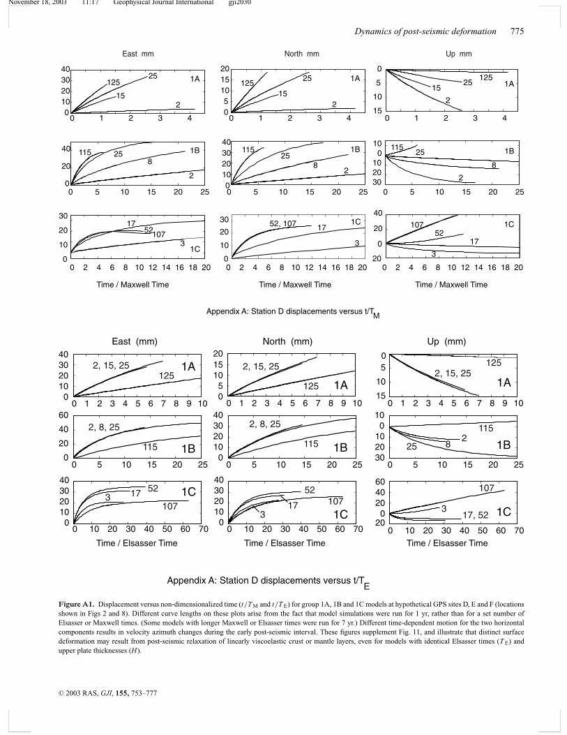
November 18, 2003 11:17 Geophysical Journal International gji2030
Dynamics of post-seismic deformation 775
Appendix A: Station D displacements versus t/T
0
20
40 1B115 258
20
10203040
1B11525
82
302010
010 115
25
8
2
010203040
1A12525
152
05
101520
1A125
25
152
15
10
5
0125
2515
2
0
10
20
30
10717
52
31C
0
10
20
30 52, 107 17
3
1C
20
0
20
40
107
1752
3
East mm North mm Up mm
0 1 2 3 40 1 2 3 40 1 2 3 4
1B
1A
1C
0 5 10 15 20 25
0 2 4 6 8 10 12 14 16 18 20
0 5 10 15 20 25
0 2 4 6 8 10 12 14 16 18 20
0 5 10 15 20 25
0 2 4 6 8 10 12 14 16 18 20
Time / Maxwell Time Time / Maxwell Time Time / Maxwell Time
M
Time / Elsasser Time
0 1 2 3 4 5 6 7 8 9 10
40
0102030 1A
0 5 10 15 20 250
20
40
60
1B
0 10 20 30 40 50 60 700
10203040
1C
East (mm)
0 1 2 3 4 5 6 7 8 9 1005
101520
0 5 10 15 20 250
10203040
0 10 20 30 40 50 60 700
10203040
Time / Elsasser Time
North (mm)
0 1 2 3 4 5 6 7 8 9 1015
10
50
Time / Elsasser Time
0 5 10 15 20 253020100
10
0 10 20 30 40 50 60 7020
0204060
Up (mm)
1A
1B
1C
1A
1B
1C
Appendix A: Station D displacements versus t/TE
2, 15, 25125
2, 15, 25
125
1252, 15, 25
2, 8, 25
825115
2, 8, 25
115
1152
3 17 52
1073
17
52107
17, 523
107
Figure A1. Displacement versus non-dimensionalized time (t/T M and t/T E) for group 1A, 1B and 1C models at hypothetical GPS sites D, E and F (locationsshown in Figs 2 and 8). Different curve lengths on these plots arise from the fact that model simulations were run for 1 yr, rather than for a set number ofElsasser or Maxwell times. (Some models with longer Maxwell or Elsasser times were run for 7 yr.) Different time-dependent motion for the two horizontalcomponents results in velocity azimuth changes during the early post-seismic interval. These figures supplement Fig. 11, and illustrate that distinct surfacedeformation may result from post-seismic relaxation of linearly viscoelastic crust or mantle layers, even for models with identical Elsasser times (T E) andupper plate thicknesses (H).
C© 2003 RAS, GJI, 155, 753–777
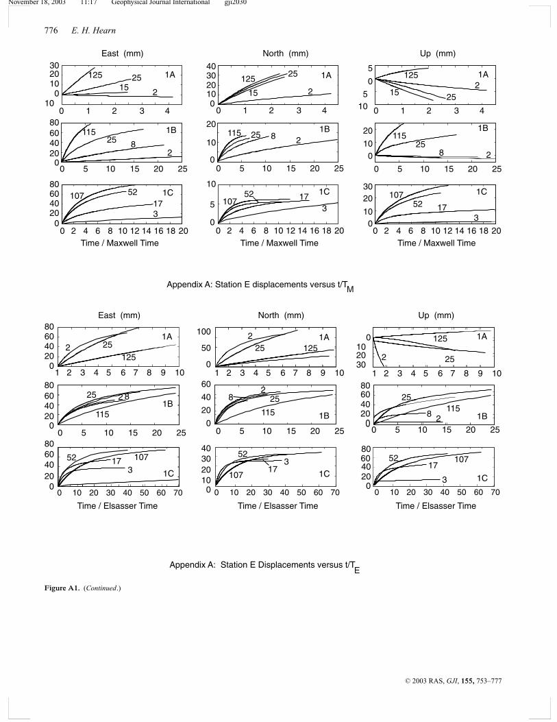
November 18, 2003 11:17 Geophysical Journal International gji2030
776 E. H. Hearn
Time / Maxwell Time Time / Maxwell Time
010
2030
202 4 6 8 10 12 14 16 180
1C10752 17
3
Time / Maxwell Time
1A12525
15 2
0 1 2 3 4 105
0
51A125
25152
0 1 2 3 4
1C107
52 173
202 4 6 8 10 12 14 16 180
1B115 25 8 2
0 5 10 15 20 250
10
20 1B115
258 2
0 5 10 15 20 25
East (mm) North (mm)
0 1 2 3 410
0102030
1A125 2515 2
20406080
0
1B11525 8
2
0 5 10 15 20 25
020406080
1C107 52173
202 4 6 8 10 12 14 16 180
Up (mm)
403020100
0
10
20
0
5
10
Appendix A: Station E displacements versus t/T.M
Time / Elsasser Time
Up (mm)
Time / Elsasser Time
0
50
100
0
20
40
60
010203040
0 10 20 30 40 50 60 70
1A12525
2
1C107
52
173
1B115
82
North (mm)
0 5 10 15 20 25
1 2 3 4 5 6 7 8 9 10
25
Time / Elsasser Time
302010
0
1C
1075217
3
1A125
252
1B115
25
8 2
0 10 20 30 40 50 60 70
0 5 10 15 20 25
1 2 3 4 5 6 7 8 9 1080604020
0
806040200
020406080
020406080
East (mm)
1A
125
252
20406080
0115
25 82
1C
10752 173
1B
0 5 10 15 20 25
0 10 20 30 40 50 60 70
1 2 3 4 5 6 7 8 9 10
Appendix A: Station E Displacements versus t/T E
Figure A1. (Continued.)
C© 2003 RAS, GJI, 155, 753–777

November 18, 2003 11:17 Geophysical Journal International gji2030
Dynamics of post-seismic deformation 777
Time / Maxwell Time
0 1 2 3 410
0102030
1A125 25
15 20
10203040
1A125
25
15 2
10
5
0
51A125
2515 2
204060
80
0
1B11525
82 5
101520
0
1B115 258 2
0 5 10 15 20 25
0
10
20 1B115
258 2
Time / Maxwell Time
2 4 6 8 10 12 14 16 18 2000
20406080
1C107 52
173
0
5
101C
10752 17
3
0
10
20
301C107
5217
3
Time / Maxwell Time
Appendix A: Station F displacements versus t/T
East (mm) North (mm) Up (mm)
0 1 2 3 4 0 1 2 3 4
0 5 10 15 20 25 0 5 10 15 20 25
2 4 6 8 10 12 14 16 18 200 2 4 6 8 10 12 14 16 18 200
M
1075217
3
0
2040
6080
1C
5217
1073
-5
0
5
10
1C
0 10 20 30 40 50 60 70
52
17
107
30
10
20
30
1C
25115
2,8
1B
0
50
100
25
115
821B
05
10
15
20
0 5 10 15 20 25
25
115
2, 8
1B
-100
102030
North mm Up mmEast mm
215
25125
010203040
1A
0 1 2 3 4 5 6 7 8 9 10
2 15 25
125
-10
-5
0
51A
215
25 125
-505
101520
1A
Appendix A: Station F displacements versus t/T
Time / Elsasser Time Time / Elsasser Time Time / Elsasser Time
0 10 20 30 40 50 60 70
0 5 10 15 20 25
0 1 2 3 4 5 6 7 8 9 10
0 10 20 30 40 50 60 70
0 5 10 15 20 25
0 1 2 3 4 5 6 7 8 9 10
E
Figure A1. (Continued.)
C© 2003 RAS, GJI, 155, 753–777