Weekly lecture notes are posted at:

http://guinness.cs.stevens.edu/%7Elbernste/  click on courses from left hand navigation

click on CS567 course name

Test Design and Techniques

A

B

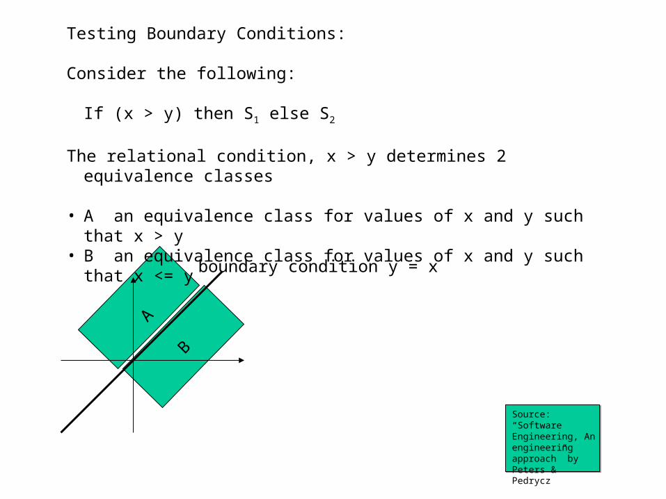
Testing Boundary Conditions:

Consider the following:

If (x > y) then S1 else S2

The relational condition, x > y determines 2 equivalence classes

• A an equivalence class for values of x and y such that x > y• B an equivalence class for values of x and y such that x <= y

boundary condition y = x

Source: “Software Engineering, An engineering approach” by Peters & Pedrycz

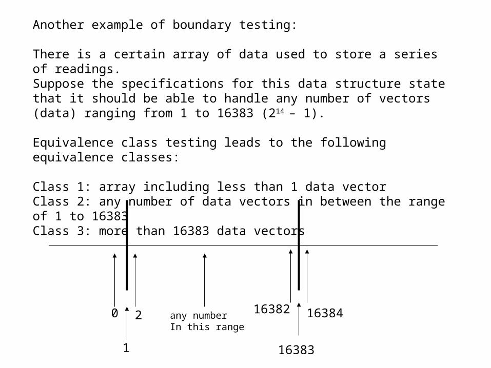
Another example of boundary testing:

There is a certain array of data used to store a series of readings.Suppose the specifications for this data structure state that it should be able to handle any number of vectors (data) ranging from 1 to 16383 (214 – 1).

Equivalence class testing leads to the following equivalence classes:

Class 1: array including less than 1 data vectorClass 2: any number of data vectors in between the range of 1 to 16383Class 3: more than 16383 data vectors

0

1

2 any numberIn this range

16382

16383

16384

Exhaustive Testing

Exhaustive testing falls under the category of black box testing. While completely impractical, it gives us a better insight into the complexity of testing and quantifies limits of practical usefulness of any brute-force approach to testing.An exhaustive test must show that the code is correct for all possible inputs.

For example: Consider a simple quadratic equationax2 + bx + c = 0 to be solved with respect to x. Here a,b,c are the parameters of the equation. The exhaustive testing starts with an internal representation of the parameters. Assume that the resolution is based on 16-bit number representation. Thus each input produces 216 different values, which in turn implies 216 test cases. Overall, we end up with 216*216*216 = 248 test cases that need to be exercised, and this is probably not feasible.

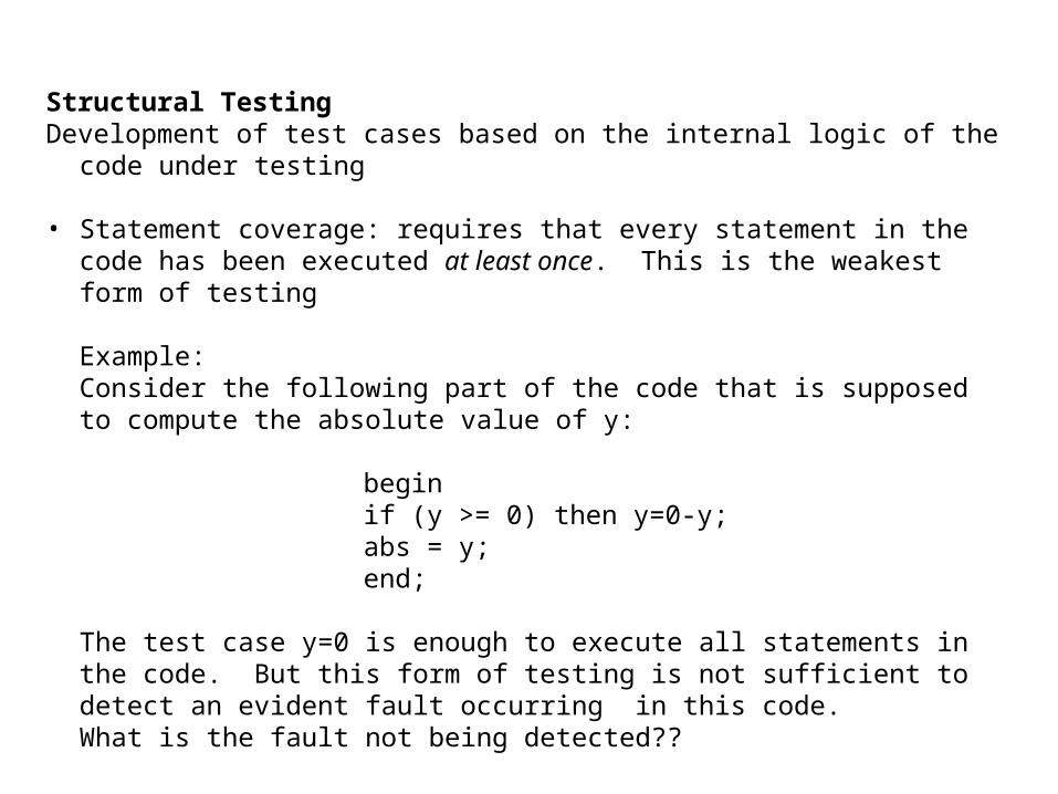
Structural TestingDevelopment of test cases based on the internal logic of the code under testing

• Statement coverage: requires that every statement in the code has been executed at least once. This is the weakest form of testing

Example:Consider the following part of the code that is supposed to compute the absolute value of y:

beginif (y >= 0) then y=0-y;abs = y;end;

The test case y=0 is enough to execute all statements in the code. But this form of testing is not sufficient to detect an evident fault occurring in this code.What is the fault not being detected??

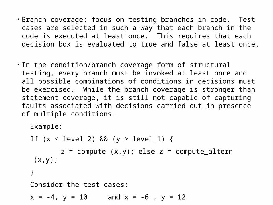
• Branch coverage: focus on testing branches in code. Test cases are selected in such a way that each branch in the code is executed at least once. This requires that each decision box is evaluated to true and false at least once.

• In the condition/branch coverage form of structural testing, every branch must be invoked at least once and all possible combinations of conditions in decisions must be exercised. While the branch coverage is stronger than statement coverage, it is still not capable of capturing faults associated with decisions carried out in presence of multiple conditions.

Example:

If (x < level_2) && (y > level_1) {

z = compute (x,y); else z = compute_altern (x,y);

}

Consider the test cases:

x = -4, y = 10 and x = -6 , y = 12

What faults are not being detected?

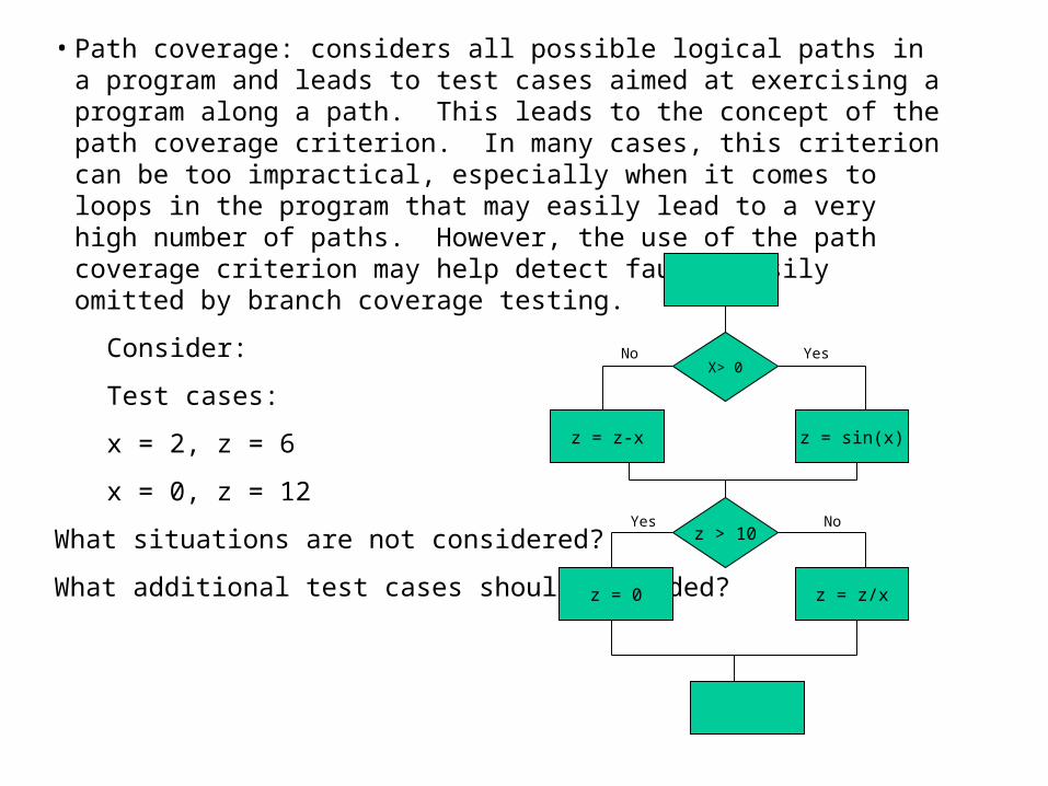
• Path coverage: considers all possible logical paths in a program and leads to test cases aimed at exercising a program along a path. This leads to the concept of the path coverage criterion. In many cases, this criterion can be too impractical, especially when it comes to loops in the program that may easily lead to a very high number of paths. However, the use of the path coverage criterion may help detect faults easily omitted by branch coverage testing.

Consider:

Test cases:

x = 2, z = 6

x = 0, z = 12

What situations are not considered?

What additional test cases should be added?

X> 0

z = z-x z = sin(x)

z > 10

z = 0 z = z/x

YesNo

Yes No

Due to the complexity of path coverage, it is essential to count and enumerate the number of paths in a program. A program does not include loops, the number of paths is determined by the number of decision nodes and their distribution. Two extreme cases that determine the bounds on the number of paths are envision in Shooman (1983). These extreme cases are:

1

2

N-1

n

Branch-merge

1

n

3

2

Branch with no merging

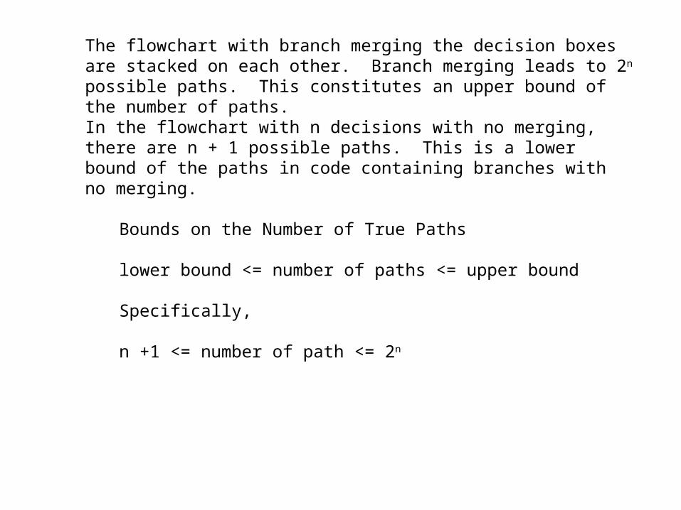
The flowchart with branch merging the decision boxes are stacked on each other. Branch merging leads to 2n possible paths. This constitutes an upper bound of the number of paths. In the flowchart with n decisions with no merging, there are n + 1 possible paths. This is a lower bound of the paths in code containing branches with no merging.

Bounds on the Number of True Paths

lower bound <= number of paths <= upper bound

Specifically,

n +1 <= number of path <= 2n

• Functional Testing

In functional testing, the specification of the software is used to identify sub-domains that should be tested. The first step is to generate a test case for every distinct type of output of the program. For example, every error message should be generated. Next, all special cases should have a test case. Tricky situations should be tested. Common mistakes and misconceptions should be tested.

See example on next page

Source: “Software Engineering” by David Gustafson

Example:

Develop a good set of test cases for a program that accepts three numbers, a, b, and c, interprets those numbers as the lengths of the sides of a triangle, and outputs the type of triangle.

What are the sub-domains we can divide the test space into?

What are the error conditions should be tested?

List your test cases!!

Creating Test Cases from the State Diagram/Table

A state machine is a behavioral model whose outcomes depends upon both previous and current input. A state transition diagram is a pictorial representation of a state machine. Its purpose is to depict the states that a system or component can assume, and it shows the events or circumstances that cause or result from a change from one state to another (IEEE 610.12)

A state transition diagram and its companion table, the state table, contain information that readily converts into test cases. The approach consists of transforming a state diagram into a state table, then creating the corresponding test cases.

Source: “Introducing to Software Testing” by Louise Tamres

When testing a state machine, a failed test can indicate any of these conditions:

1. A state shown on the state diagram is missing from the code

2. A transaction shown on the state diagram is missing from the code

3. A transaction results in the wrong state

4. A state performs the wrong function

Example: Develop test cases for a stopwatchThe state diagram for the stopwatch consists of three states and the interfaces contains three inputs and one output. Each of the three inputs in an event that affects the system. They are:

INPUTStart: continue to increment elapsed time from the currently display time. The time value increases once every second

Stop: stop incrementing the elapsed time and display the last time value

Reset: reset current time to 0

OUTPUTTime: current time value

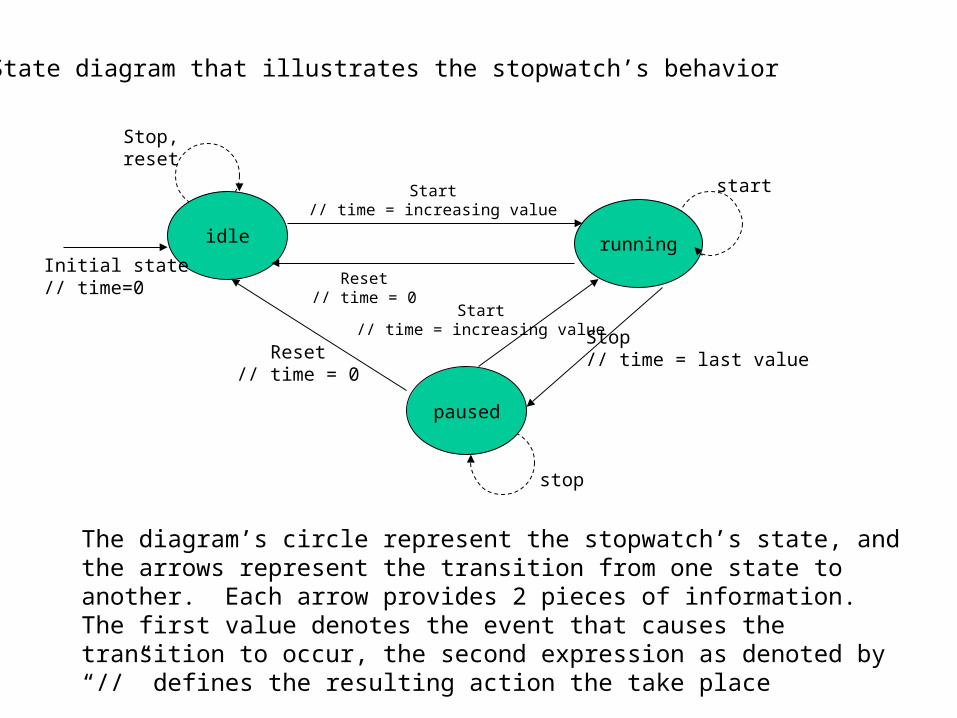
State diagram that illustrates the stopwatch’s behavior

idle running

paused

Stop,reset

Initial state// time=0

Start// time = increasing value

Reset// time = 0

start

Stop// time = last value

Start// time = increasing value

Reset// time = 0

stop

The diagram’s circle represent the stopwatch’s state, and the arrows represent the transition from one state to another. Each arrow provides 2 pieces of information. The first value denotes the event that causes the transition to occur, the second expression as denoted by “//” defines the resulting action the take place

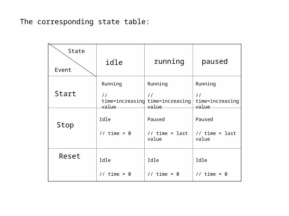
The corresponding state table:

Idle

// time = 0

Paused

// time = last value

Paused

// time = last value

Idle

// time = 0

Idle

// time = 0

Idle

// time = 0

State

Event

Start

Stop

Reset

idle running paused

Running

// time=increasing value

Running

// time=increasing value

Running

// time=increasing value

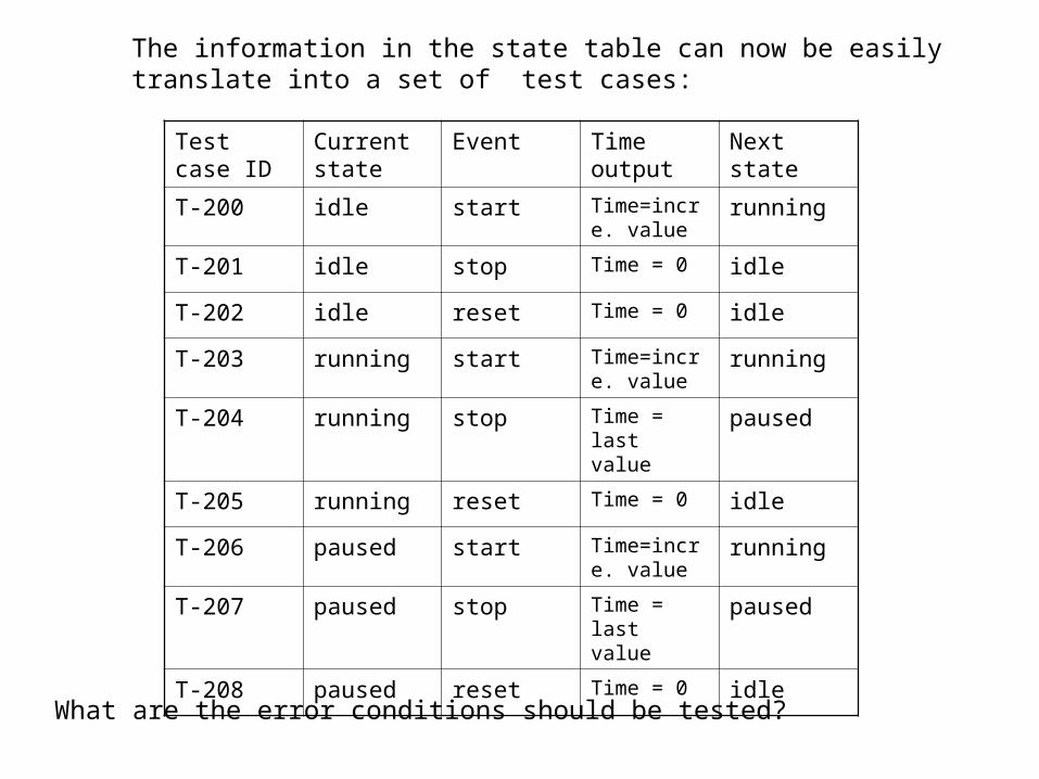
The information in the state table can now be easily translate into a set of test cases:

Test case ID

Current state

Event Time output

Next state

T-200 idle start Time=incre. value

running

T-201 idle stop Time = 0 idle

T-202 idle reset Time = 0 idle

T-203 running start Time=incre. value

running

T-204 running stop Time = last value

paused

T-205 running reset Time = 0 idle

T-206 paused start Time=incre. value

running

T-207 paused stop Time = last value

paused

T-208 paused reset Time = 0 idle

What are the error conditions should be tested?

“Using Simplicity to Control Complexity”** by Prof. Sha, 2001

Why is keeping systems simple so difficult?

One reason involves the pursuit of features and performance. Gaining higher performance and functionality requires that we push the technology envelope and stretch the limits of our understanding.Avoiding complex software components is not practical in most applications today.

We need an approach that let us safely exploit the features the applications provide.

For example:

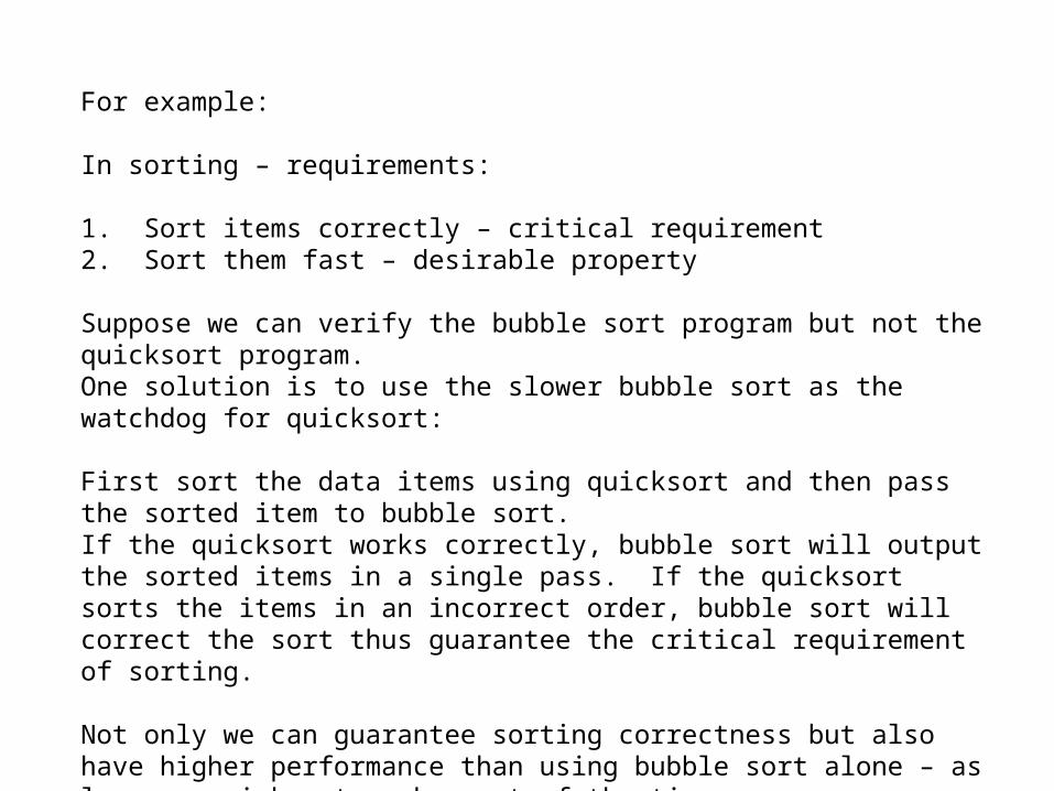
In sorting – requirements:

1. Sort items correctly – critical requirement2. Sort them fast – desirable property

Suppose we can verify the bubble sort program but not the quicksort program.One solution is to use the slower bubble sort as the watchdog for quicksort:

First sort the data items using quicksort and then pass the sorted item to bubble sort.If the quicksort works correctly, bubble sort will output the sorted items in a single pass. If the quicksort sorts the items in an incorrect order, bubble sort will correct the sort thus guarantee the critical requirement of sorting.

Not only we can guarantee sorting correctness but also have higher performance than using bubble sort alone – as long as quicksort works most of the time.

“We can exploit the features and performance of complex software even if we cannot verify them, provided that we can guarantee the critical requirements with simple software”

Prof. Sha (2001)

Software testing consumes 30% to 40% of an organization’s software development resources. But, still many faults remain undetected and are later found in the field. This often cause customer dissatisfaction, high field maintenance cost, and perception of poor product quality.

To improve customer satisfaction and reduce development costs, it is imperative that the software teams reduce testing costs, reduce product introduction delays and send fewer faults to the field.

We need to find and plan more efficient software tests!!!

Testing effectiveness can be improved by:

• automating the testing activity so that one software program tests another program and collects the results.

• wisely determine which tests should be run.

The Robust Testing method uses the mathematical tool of orthogonal arrays (OAs) to select the test cases intelligently. It addresses an important task in testing, namely, deciding what tests to conduct so that faults can be detected with minimum resources.

Dr. Genichi Taguchi is the pioneer in the Robust Design method.

Orthogonal arrays, which are also called Latin Squares.

Taguchi has tabulated 18 basic orthogonal arrays that we call standard orthogonal arrays.

Source: “Quality Engineering using Robust Design” by Madhav Phadke

The first step in constructing an orthogonal array to fit a specific case study is to calculate the minimum number of tests that must be performed -- this is also called degrees of freedom

•One degree of freedom is associated with the overall mean regardless of the number of parameters to be tested.

•The number of degrees of freedom associated with a factor (parameter) is equal to one less than the number of levels for that factor.

•The degrees of freedom associated with interaction between two factors A and B, are given by the product of the degrees of freedom for each of the two factors.

Degrees of freedom for interaction A x B

= (degrees of freedom for A) x (degrees of freedom for B)

Example:

Suppose a case study has one 2-level factor (parameter) A, five 3-level factors (B, C, D, E, F), and we are interested in estimating the the interaction A x B. The degrees of freedom for this experiment are the computed as follows:

Factor/Interaction Degrees of freedom

Overall mean 1A 2 – 1 = 1B, C, D, E, F 5 x (3 – 1) = 10A x B (2 – 1) x (3 –1) = 2

Total 14

We must conduct at least 14 experiments to be able to estimate the effect of each factor and the desired interaction

Example:

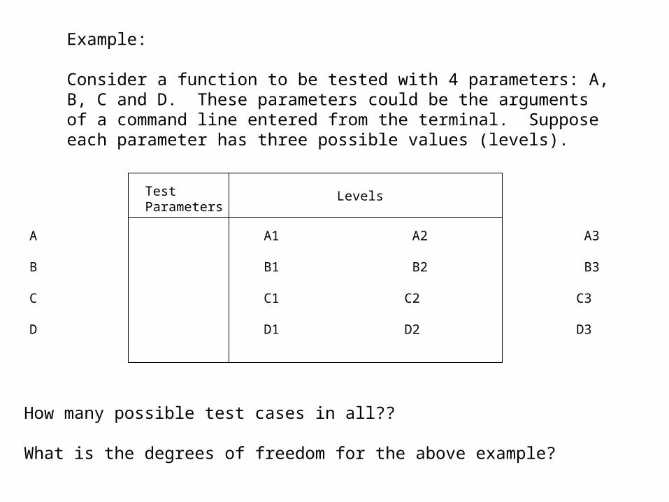
Consider a function to be tested with 4 parameters: A, B, C and D. These parameters could be the arguments of a command line entered from the terminal. Suppose each parameter has three possible values (levels).

TestParameters

Levels

A A1 A2 A3

B B1 B2 B3

C C1 C2 C3

D D1 D2 D3

How many possible test cases in all??

What is the degrees of freedom for the above example?

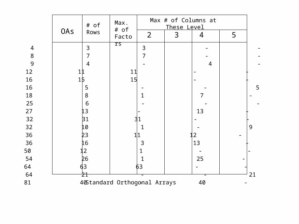
OAs# of Rows

Max.# of Factors

Max # of Columns at These Level

2 3 4 5

L4 4 3 3 - - -L8 8 7 7 - - -L9 9 4 - 4 - -L12 12 11 11 - - -L16 16 15 15 - - -L’16 16 5 - - 5 -L18 18 8 1 7 - -L25 25 6 - - - 6L27 27 13 - 13 - -L32 32 31 31 - - -L’32 32 10 1 - 9 -L36 36 23 11 12 - -L’36 36 16 3 13 - -L50 50 12 1 - - 11L54 54 26 1 25 - -L64 64 63 63 - - -L’64 64 21 - - 21 -L81 81 40 - 40 - -Standard Orthogonal Arrays

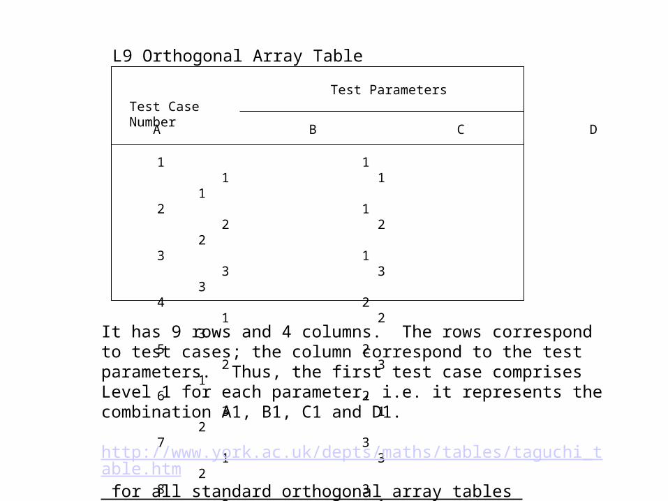
L9 Orthogonal Array Table

Test CaseNumber

Test Parameters

A B C D

1 1 1 1 1

2 1 2 2 2

3 1 3 3 3

4 2 1 2 3

5 2 2 3 1

6 2 3 1 2

7 3 1 3 2

8 3 2 1 3

9 3 3 2 1

It has 9 rows and 4 columns. The rows correspond to test cases; the column correspond to the test parameters. Thus, the first test case comprises Level 1 for each parameter, i.e. it represents the combination A1, B1, C1 and D1.

http://www.york.ac.uk/depts/maths/tables/taguchi_table.htm for all standard orthogonal array tables

An orthogonal array has the balancing property, for each pair of columns, all parameter level combinations occur an equal number of times

By conducting the nine tests indicated by L9, we can detect:

•Any consistent problem with any level of any single parameter. For example, if all cases of parameter A at Level A1 cause error condition, it is a single-mode failure, tests 1,2, and 3 will show errors.•Any consistent problem with pairwise compatibility of parameters

Orthogonal array-based test cases cannot prove that a product will work for all possible parameter-level combinations. But the pairwise balancing property gives excellent coverage of the entire test domain defined by the test parameters.

A thorough analysis of the requirements documents and understanding of the usage of the software is needed to prepare the parameter-level table.

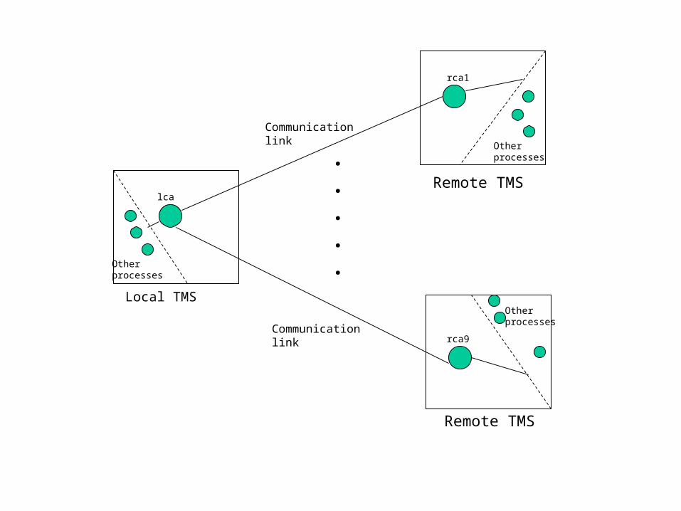
Example:

Ten Transport Maintenance Systems (TMS) are interconnected in a ring topology. There is one Local TMS who is responsible for collecting alarms from all remote TMSs. Inter TMS communication is handled via a special process. The process architecture mainly comprises 2 types of communicators: the local communicator (lca) resides on the local TMS and the remote communicators (rca’s) reside on the remote TMSs. We have to test for a local TMS communicating with a maximum of 9 remote TMSs. We want to test the ability to turn on or off receiving alarms from remote TMSs by turning on or off the rca’s. Use the Orthogonal Arrays technique to design the test cases to test this feature. 

Otherprocesses

Otherprocesses

Otherprocesses

.

.

.

.

.

Communicationlink

Communicationlink

lca

rca1

rca9

Local TMS

Remote TMS

Remote TMS

Homework week 2 (1/27):

1. Work on the questions asked throughout this lecture

2. Read chapters 4,5