Embed Size (px)
Citation preview

Week 16
Multiple Equation Models
Rich Frank
University of New Orleans
December 6, 2012

Also known as simultaneous equation models or systems of equations.
Why on earth would we ever want to use these models?
Theory!
We have reason to believe that our data violate the assumptions underlying the other models we have seen this semester.
Multiple equation models
MLE Class 16 2
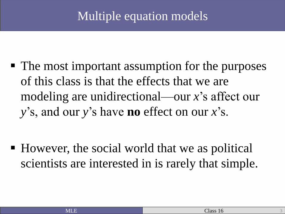
The most important assumption for the purposes
of this class is that the effects that we are
modeling are unidirectional—our x’s affect our
y’s, and our y’s have no effect on our x’s.
However, the social world that we as political
scientists are interested in is rarely that simple.
Multiple equation models
MLE Class 16 3

We have already begun relaxing the assumption that
one equation can adequately approximate the
phenomena we are interested in.
Therefore, we have already become familiar with
multiple equation models including the ZIP, ZINB,
Heckman, and other selection models.
Therefore, this class is but another effort at relaxing
restrictive assumptions we have made in the past.
MLE Class 16 4

One of the most important of these assumptions
(dating back to 6002) is that our x’s are unrelated
to our error term, ε.
MLE Class 16 5
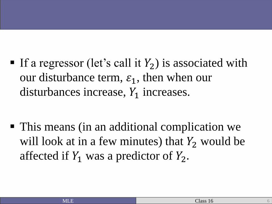
If a regressor (let’s call it 𝑌2) is associated with
our disturbance term, 𝜀1, then when our
disturbances increase, 𝑌1 increases.
This means (in an additional complication we
will look at in a few minutes) that 𝑌2 would be
affected if 𝑌1 was a predictor of 𝑌2.
MLE Class 16 6

For example, think about economic development
and democracy.
There is a large literature suggesting that
economically developed states are more likely to
be democratic.
MLE Class 16 7

MLE Class 16 8
Democracy
𝜀
Development

In this example, 𝜀 includes everything else
besides economic development that can cause
democracy.
One such factor that can effect democracy could
be the government’s decision to repress its
citizens.
MLE Class 16 9

MLE Class 16 10
Democracy
𝜀 + Repression
Development

But repression can also affect corporations and
citizens from wanting to invest in their future.
People might be more worried about whether
security forces are going to throw them out of a
helicopter than on starting a new business.
MLE Class 16 11

Another popular example is the relationship between party affiliation and candidate evaluations.
The positions that candidates have can affect what party they join as well as how they are evaluated.
You can also model these types of theoretical relationships.
MLE Class 16 12

The path diagram should look more like this
MLE Class 16 13
Democracy
𝜀 + Repression
Development

Or this
MLE Class 16 14
Candidate
evaluations
𝜀 + Policy positions
Party ID

In notation
MLE Class 16 15
𝑌2
𝜀1
𝑌1

This means that 𝑌2, economic development, is an
endogenous regressor, because it arises in a
system where it is related to 𝜀.
A variable that affects democracy (say distance
from Geneva) but does not affect economic
development would be considered exogenous.
MLE Class 16 16

If we just run a single equation predicting democracy without taking into account what we know about the reciprocal nature of the relationship between democracy and development, then our OLS estimators would be inconsistent.
Remember, an estimate is considered consistent if as our sample approaches the size of the population our parameter value approximates the population’s value.
MLE Class 16 17

Therefore in order to get consistent and efficient estimators, we need to take into account what we theoretically know about the world and model this endogeneity.
This simple example and path diagram hints that there are a large number of potential models that can be adjusted or tweaked to fit the theoreticalmodel (path diagram) that we think explains the world.
MLE Class 16 18

We will explore several of the most
straightforward and popular models today.
First, the adjustments we need to make about the
distribution of our errors given our theoretical model.
And then explicitly model these endogenous effects.
MLE Class 16 19

A basic structure of equations can be written as follows:
𝑌1 = 𝛽01 + 𝛽11𝑌2 + 𝜷𝒎𝑿𝒎 + 𝜀1
𝑌2 = 𝛽02 + 𝜷𝒌𝑿𝒌 + 𝜀2
Where 𝑿𝒎 represents a vector of variables that affect 𝑌1, and 𝑿𝒌 represents a vector of variables that affect 𝑌2.
And m and k are >0
MLE Class 16 20

MLE Class 16 21
𝑌2
𝜀1
𝑌1
𝑋𝑘 𝑋𝑚
𝜀2

To obtain a consistent parameter estimate, we assume that 𝜀1 is uncorrelated with 𝑿𝒎 but are correlated with 𝑌2.
In order to estimate the model we also need at least k variables that satisfy the assumption that 𝐸(𝜀1| 𝑿𝒌 ) = 0.
These k variables therefore have to provide some information about 𝑌2 but have no effect on 𝜀1.
MLE Class 16 22

This model is relatively simple to estimate
because all the arrows point in one direction (uni-
directional).
The models are hierarchical.
This type of model is called recursive.
MLE Class 16 23

However, there are many instances where these assumptions are non-realistic.
Going back to my development and democracy example, it has been argued that democracies are more likely to attract investment and development because they are perceived to be more stable or have clearer rules and institutional decision-making.
Therefore, development affects democracy at the same time that democracy affects development.
MLE Class 16 24

We could therefore write a more complicated
non-recursive system of equations:
𝑌1 = 𝛽01 + 𝛽11𝑌2 + 𝜷𝒎𝑿𝒎 + 𝜀1
𝑌2 = 𝛽02 + 𝛽12𝑌1 + 𝜷𝒌𝑿𝒌 + 𝜀2
Non-recursive models
MLE Class 16 25

Here, arrows go both directions.
MLE Class 16 26
𝑌2
𝜀1
𝑌1
𝑋𝑘 𝑋𝑚
𝜀2

If the system is recursive, then you can run the
models for 𝑌1 and 𝑌2 independently.
This is considered a limited information approach
because we are not using all the information we
have on what we know about the world.
Limited information models
MLE Class 16 27

As Greene (2008: 361-2) discusses, if there exists
more than one theory that can lead to the same
observed data (observational equivalence), then
the model structure is unidentified.
Simultaneous equation models are considered one
of three types:
Under-identified
Identified
Over-identified
The identification problem
MLE Class 16 28
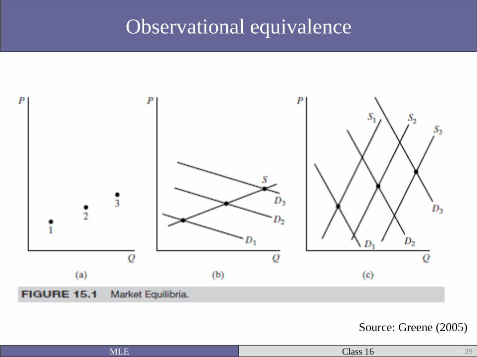
Observational equivalence
MLE Class 16 29
Source: Greene (2005)

A necessary (but not sufficient) condition for identification is that:
“In a model of M simultaneous equations in order for an equation to be identified, it must exclude at least M - 1 variables (endogenous as well as predetermined [exogenous]) appearing in the model. If it excludes exactly M -1 variables, the equation is just identified. If it excludes more than M -1 variables, it is overidentified,”
-Gujarati (2003: 748)
Order condition for identification
MLE Class 16 30

Coefficients
Intercept Y1 Y2 X1 X2
Y1 B01 1 B12 B13 0
Y2 B02 0 1 0 B23
It is easiest to use a table of coefficients
MLE Class 16 31

The order condition, you will notice, is necessary,
but it is not sufficient to identify a model.
There will be at least one solution, but there could
be more than one.
We need another condition that is sufficient for
uniqueness.
Rank Condition for Identification
MLE Class 16 32

“In a model containing M equations in M
endogenous variables, an equation is identified if
and only if at least one nonzero determinant of
order (M - 1)(M - 1) can be constructed from the
coefficients of the variables (both endogenous
and predetermined) excluded from that particular
equation but included in the other equations of
the model,”
Gujarati (2003: 750)
Rank Condition for Identification
MLE Class 16 33

The rank order condition involves establishing matrices of the excluded variables of a particular equation that are included in another equation.
This would take an additional class to explain to my (and probably your satisfaction).
Suffice it to say that there is a means of establishing the rank order condition manually, and Stata will reject your model if it is not at least identified.
Let’s move on to estimating models with endogenous regressors.
MLE Class 16 34

Developed independently by Theil (1953) and Basmann (1957).
For example, take our non-recursive model above where 𝑌1 and 𝑌2(democracy and development, say) were functions of each other.
Stage 1: Regress 𝑌1 on all exogenous variables in the system. This gives you the 𝑌1 and 𝜀.
Stage 2: Plug in the predicted 𝑌1 ( 𝑌1 + 𝜀). This estimates an error term that includes the estimated error 𝜀1 and 𝜀2.
Substantively what this does is asymptotically “purify” 𝑌1 from the effect of 𝜀2.
This enables us to get consistent estimates as our sample size increases towards the population size.
Two-Stage Lease Squares (2SLS)
MLE Class 16 35

Stage 1: Same as for 2SLS, but for all equations.
Stage 2: Estimate covariance matrix of
disturbances from the Stage 1 estimates of all the
endogenous regressors models
Stage 3: Using the Stage 2 matrix plug in the
instrumented variable values rather than the
endogenous variables.
Three-stage Lease Squares (3SLS)
MLE Class 16 36
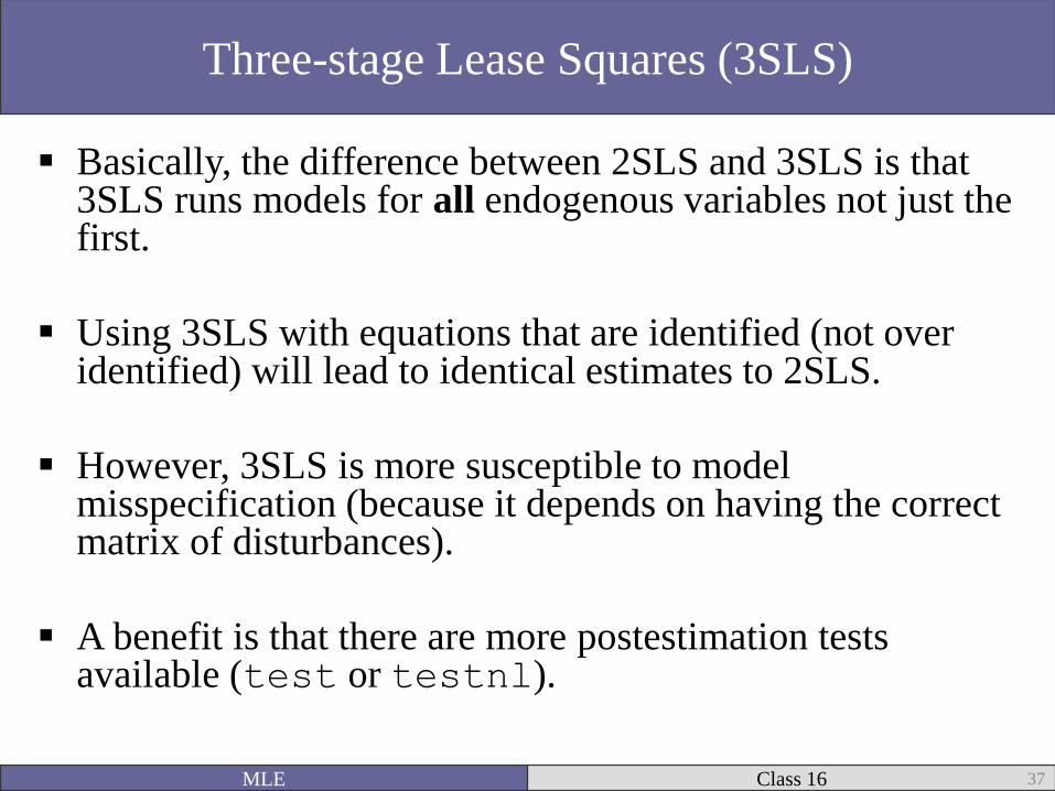
Basically, the difference between 2SLS and 3SLS is that 3SLS runs models for all endogenous variables not just the first.
Using 3SLS with equations that are identified (not over identified) will lead to identical estimates to 2SLS.
However, 3SLS is more susceptible to model misspecification (because it depends on having the correct matrix of disturbances).
A benefit is that there are more postestimation tests available (test or testnl).
Three-stage Lease Squares (3SLS)
MLE Class 16 37

Let’s try some examples…
Namely, the interrelationship between democracy
and development using Fearon and Laitin’s
(2003) data.
MLE Class 16 38

. reg polity2 gdpenl colbrit mtnest Oil ef warl, robust cluster(ccode)
Linear regression Number of obs = 6243
F( 6, 152) = 11.26
Prob > F = 0.0000
R-squared = 0.2254
Root MSE = 6.6845
(Std. Err. adjusted for 153 clusters in ccode)
------------------------------------------------------------------------------
| Robust
polity2 | Coef. Std. Err. t P>|t| [95% Conf. Interval]
-------------+----------------------------------------------------------------
gdpenl | .6320265 .2112486 2.99 0.003 .2146639 1.049389
colbrit | 2.192107 .976455 2.24 0.026 .2629305 4.121283
mtnest | .0065496 .0191193 0.34 0.732 -.0312243 .0443235
Oil | -5.102077 1.247602 -4.09 0.000 -7.566957 -2.637198
ef | -4.433521 1.916182 -2.31 0.022 -8.21931 -.6477328
warl | 1.556295 .8451118 1.84 0.067 -.113387 3.225977
_cons | -.8329061 1.597662 -0.52 0.603 -3.989398 2.323585
------------------------------------------------------------------------------
. est store P_OLS
Polity without controlling for endogeneity
MLE Class 16 39

ivregress 2sls polity2 colbrit mtnest Oil ef warl (gdpenl = Oil year muslim relfrac), ///
> first robust cluster(ccode)
First-stage regressions
-----------------------
Number of obs = 6243
N. of clusters = 153
F( 8, 6234) = 13.32
Prob > F = 0.0000
R-squared = 0.2034
Adj R-squared = 0.2024
Root MSE = 3.9505
------------------------------------------------------------------------------
| Robust
gdpenl | Coef. Std. Err. t P>|t| [95% Conf. Interval]
-------------+----------------------------------------------------------------
colbrit | 1.329785 .7243687 1.84 0.066 -.0902269 2.749798
mtnest | -.0069368 .0144117 -0.48 0.630 -.0351887 .021315
Oil | 3.25208 .9360339 3.47 0.001 1.417131 5.087029
ef | -4.67675 .9701836 -4.82 0.000 -6.578644 -2.774856
warl | -1.919467 .5477171 -3.50 0.000 -2.993181 -.845753
year | .0646421 .0094885 6.81 0.000 .0460414 .0832428
muslim | -.0111938 .0070446 -1.59 0.112 -.0250037 .0026161
relfrac | 2.248686 1.475143 1.52 0.127 -.6431015 5.140474
_cons | -122.8343 18.38209 -6.68 0.000 -158.8695 -86.79907
------------------------------------------------------------------------------
With 2SLS: first stage
MLE Class 16 40

Instrumental variables (2SLS) regression Number of obs = 6243
Wald chi2(6) = 66.39
Prob > chi2 = 0.0000
R-squared = 0.0445
Root MSE = 7.4198
(Std. Err. adjusted for 153 clusters in ccode)
------------------------------------------------------------------------------
| Robust
polity2 | Coef. Std. Err. z P>|z| [95% Conf. Interval]
-------------+----------------------------------------------------------------
gdpenl | 1.417127 .2935135 4.83 0.000 .8418509 1.992403
colbrit | .920523 1.327838 0.69 0.488 -1.681991 3.523037
mtnest | .015147 .0163096 0.93 0.353 -.0168192 .0471133
Oil | -7.323945 2.100681 -3.49 0.000 -11.4412 -3.206686
ef | -1.125375 1.70013 -0.66 0.508 -4.457568 2.206818
warl | 2.805521 .9799865 2.86 0.004 .8847828 4.726259
_cons | -4.921945 1.717969 -2.86 0.004 -8.289102 -1.554787
------------------------------------------------------------------------------
Instrumented: gdpenl
Instruments: colbrit mtnest Oil ef warl year muslim relfrac
. est store P_2SLS
Second stage
MLE Class 16 41

. est table P_OLS P_2SLS, b(%9.5f) se
--------------------------------------
Variable | P_OLS P_2SLS
-------------+------------------------
gdpenl | 0.63203 1.41713
| 0.21125 0.29351
colbrit | 2.19211 0.92052
| 0.97646 1.32784
mtnest | 0.00655 0.01515
| 0.01912 0.01631
Oil | -5.10208 -7.32394
| 1.24760 2.10068
ef | -4.43352 -1.12538
| 1.91618 1.70013
warl | 1.55630 2.80552
| 0.84511 0.97999
_cons | -0.83291 -4.92194
| 1.59766 1.71797
--------------------------------------
legend: b/se
Notice the difference in GDP’s Beta
MLE Class 16 42
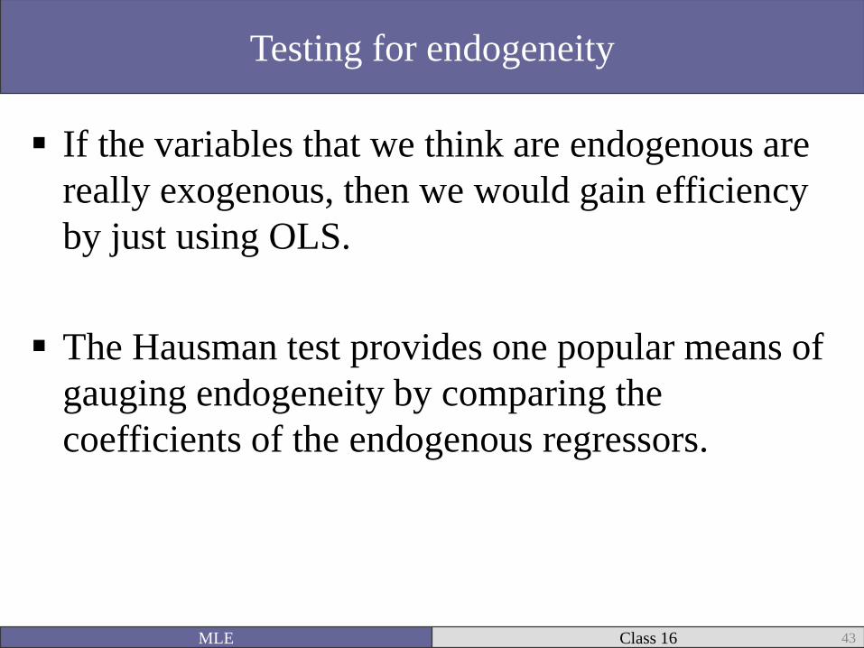
If the variables that we think are endogenous are
really exogenous, then we would gain efficiency
by just using OLS.
The Hausman test provides one popular means of
gauging endogeneity by comparing the
coefficients of the endogenous regressors.
Testing for endogeneity
MLE Class 16 43

For one (potentially) endogenous variable, the
Hausman (1978) test statistic is:
𝑇𝐻 =( 𝛽𝐼𝑉 − 𝛽𝑂𝐿𝑆)2
𝑉( 𝛽𝐼𝑉 − 𝛽𝑂𝐿𝑆)
This test statistic is distributed chi-squared with 1
degree of freedom.
Testing for endogeneity
MLE Class 16 44

. estat endogenous, forcenonrobust
Tests of endogeneity
Ho: variables are exogenous
Durbin (score) chi2(1) = 123.603 (p = 0.0000)
Wu-Hausman F(1,6235) = 125.938 (p = 0.0000)
Stata also reports a Durbin test statistic, which
assumes exogeneity and tests for endogeneity (the
opposite of the Hausman).
Testing for endogeneity
MLE Class 16 45

. estat firststage
First-stage regression summary statistics
--------------------------------------------------------------------------
| Adjusted Partial
Variable | R-sq. R-sq. R-sq. F(3,6234) Prob > F
-------------+------------------------------------------------------------
gdpenl | 0.2034 0.2024 0.0782 176.221 0.0000
--------------------------------------------------------------------------
Minimum eigenvalue statistic = 176.221
Critical Values # of endogenous regressors: 1
Ho: Instruments are weak # of excluded instruments: 3
---------------------------------------------------------------------
| 5% 10% 20% 30%
2SLS relative bias | 13.91 9.08 6.46 5.39
-----------------------------------+---------------------------------
| 10% 15% 20% 25%
2SLS Size of nominal 5% Wald test | 22.30 12.83 9.54 7.80
LIML Size of nominal 5% Wald test | 6.46 4.36 3.69 3.32
---------------------------------------------------------------------
First stage diagnostics
MLE Class 16 46

The partial R-squared is the variance that is explained by the instruments after controlling for the endogeneity.
The F statistic is for the joint significance for the instruments.
There is a rule of thumb that suggests you have strong instruments if the F statistic is greater than 10.
First stage diagnostics
MLE Class 16 47
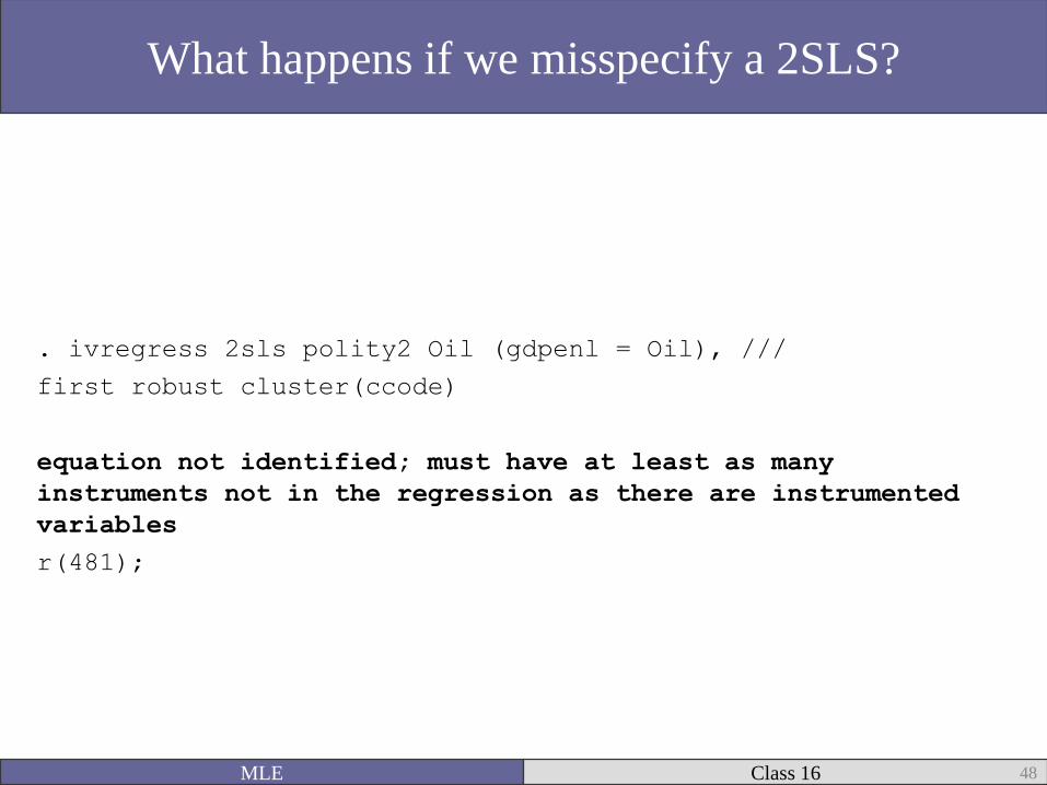
. ivregress 2sls polity2 Oil (gdpenl = Oil), ///
first robust cluster(ccode)
equation not identified; must have at least as many
instruments not in the regression as there are instrumented
variables
r(481);
What happens if we misspecify a 2SLS?
MLE Class 16 48
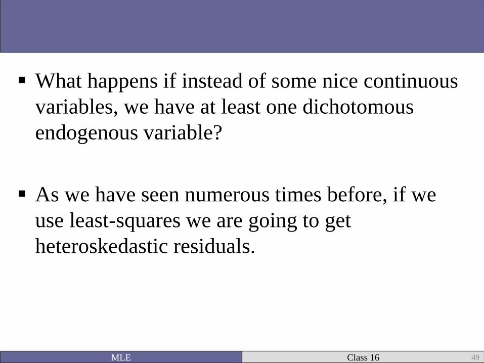
What happens if instead of some nice continuous
variables, we have at least one dichotomous
endogenous variable?
As we have seen numerous times before, if we
use least-squares we are going to get
heteroskedastic residuals.
MLE Class 16 49

You could ignore them…
But we know better than to do that because it
would lead to biased and inconsistent estimates.
MLE Class 16 50

Let’s try dichotomizing Polity into a dummy variable called dichotomous, which equals 1 if Polity>5.
. est table P_OLS P_2SLS dich, b(%9.5f) se
--------------------------------------------------
Variable | P_OLS P_2SLS dich
-------------+------------------------------------
gdpenl | 0.63203 1.41713 0.08864
| 0.02058 0.08169 0.01773
colbrit | 2.19211 0.92052 0.06584
| 0.19898 0.25479 0.07956
mtnest | 0.00655 0.01515 0.00012
| 0.00414 0.00467 0.00089
Oil | -5.10208 -7.32394 -0.39356
| 0.26408 0.36768 0.11452
ef | -4.43352 -1.12538 -0.11566
| 0.34296 0.50411 0.10113
warl | 1.55630 2.80552 0.13521
| 0.25690 0.31127 0.06864
_cons | -0.83291 -4.92194 0.08405
| 0.21460 0.47286 0.10240
--------------------------------------------------
legend: b/se
MLE Class 16 51

In addition to running ivregress using 2SLS , you can also specify LIML or GMM.
These are different means of specifying the βs, and are outside the scope of what I am trying to cover today.
GMM is a popular alternative to OLS that estimates a parameter by substituting a population parameter (say μ) with its sample equivalent.
𝐸 𝑦 − 𝜇 = 0
𝜇 =1
𝑁
𝑖=1
𝑁
𝑦𝑖
MLE Class 16 52

Also referred to as the least-variance ratio.
More computationally intensive (you do not want
to see the likelihood function).
Its main benefit is its invariance to the
normalization of the equation (Greene 2008:
375).
Limited Information Maximum Likelihood (LIML)
MLE Class 16 53

. est table P_OLS P_2SLS Three, b(%9.5f) se
--------------------------------------------------
Variable | P_OLS P_2SLS Three
-------------+------------------------------------
_ |
gdpenl | 0.63203 1.41713
| 0.02058 0.08169
colbrit | 2.19211 0.92052
| 0.19898 0.25479
mtnest | 0.00655 0.01515
| 0.00414 0.00467
Oil | -5.10208 -7.32394
| 0.26408 0.36768
ef | -4.43352 -1.12538
| 0.34296 0.50411
warl | 1.55630 2.80552
| 0.25690 0.31127
_cons | -0.83291 -4.92194
| 0.21460 0.47286
-------------+------------------------------------
polity2 |
gdpenl | 1.46536
| 0.08137
colbrit | 2.18466
| 0.23449
mtnest | 0.00839
| 0.00420
Oil | -7.17073
| 0.36703
ef | -3.82107
| 0.48275
warl | 1.52645
| 0.28745
_cons | -3.94269
| 0.46807
-------------+------------------------------------
gdpenl |
Oil | 3.43087
| 0.16846
year | 0.05038
| 0.00353
muslim | -0.03048
| 0.00144
relfrac | 0.44866
| 0.23119
_cons | -95.71524
| 6.96376
--------------------------------------------------
legend: b/se
Let’s try using 3SLS
MLE Class 16 54
Notice the slightly
larger coefficient.

Let’s get back to our dichotomous variable
problem.
Suppose that we have one dichotomous variable
and one continuous variable.
MLE Class 16 55

Going back to our old two endogenous variable model:
𝑌1 = 𝛽01 + 𝛽11𝑌2 + 𝜷𝒎𝑿𝒎 + 𝜀1
𝑌2 = 𝛽02 + 𝛽12𝑌1 + 𝜷𝒌𝑿𝒌 + 𝜀2
Let’s assume that 𝑌1 is observed dichotomously, where we are interested in the latent continuous variable 𝑌1*:
𝑌1𝑖 = 0 𝑖𝑓 𝑌1∗ < 0
1 𝑖𝑓 𝑌1∗ ≥ 0
MLE Class 16 56

This multi-equation instrumental variable model
can now be estimated using maximum likelihood.
MLE Class 16 57

From Stata 11 Base Reference Manual: 733.
Let’s try this function on some real data.
The ivprobit likelihood function
MLE Class 16 58
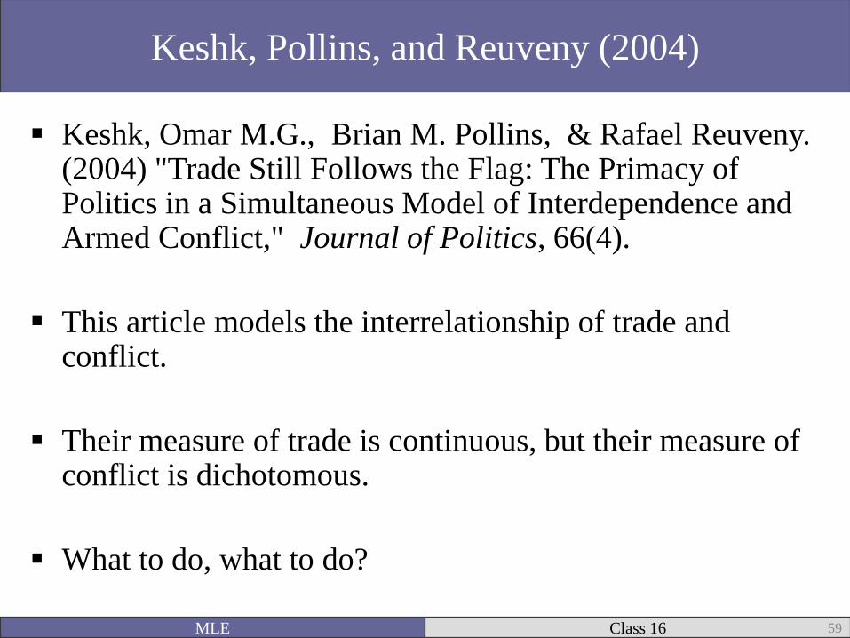
Keshk, Omar M.G., Brian M. Pollins, & Rafael Reuveny. (2004) "Trade Still Follows the Flag: The Primacy of Politics in a Simultaneous Model of Interdependence and Armed Conflict," Journal of Politics, 66(4).
This article models the interrelationship of trade and conflict.
Their measure of trade is continuous, but their measure of conflict is dichotomous.
What to do, what to do?
Keshk, Pollins, and Reuveny (2004)
MLE Class 16 59

. ivprobit dispute dispute_lag dependence lower_growth lower_democracy alliances capability_ratio //
> (trade = trade_lag gdp_A gdp_B pop_A pop_B distance lower_democracy alliances ), robust cluster(cluster)
Fitting exogenous probit model
Iteration 6: log likelihood = -3500.0329
Fitting full model
Iteration 3: log pseudolikelihood = -266825.03
Probit model with endogenous regressors Number of obs = 143792
Wald chi2(7) = 1676.10
Log pseudolikelihood = -266825.03 Prob > chi2 = 0.0000
(Std. Err. adjusted for 6636 clusters in cluster)
------------------------------------------------------------------------------
| Robust
| Coef. Std. Err. z P>|z| [95% Conf. Interval]
-------------+----------------------------------------------------------------
trade | .0382846 .0038199 10.02 0.000 .0307978 .0457714
dispute_lag | 2.480361 .0833551 29.76 0.000 2.316988 2.643734
dependence | -59.12915 27.28599 -2.17 0.030 -112.6087 -5.649594
lower_growth | -.0073218 .0041565 -1.76 0.078 -.0154684 .0008248
lower_demo~y | -.1500483 .0205881 -7.29 0.000 -.1904003 -.1096964
alliances | .3252931 .0551563 5.90 0.000 .2171888 .4333973
capability~o | -.0001679 .0001581 -1.06 0.289 -.0004778 .0001421
_cons | -2.852112 .0481366 -59.25 0.000 -2.946458 -2.757766
-------------+----------------------------------------------------------------
/athrho | -.1284848 .0190344 -6.75 0.000 -.1657914 -.0911781
/lnsigma | .412911 .0063298 65.23 0.000 .4005047 .4253172
-------------+----------------------------------------------------------------
rho | -.1277824 .0187236 -.1642889 -.0909263
sigma | 1.51121 .0095657 1.492578 1.530076
------------------------------------------------------------------------------
Instrumented: trade
Instruments: dispute_lag dependence lower_growth lower_democracy alliances
capability_ratio trade_lag gdp_A gdp_B pop_A pop_B distance
------------------------------------------------------------------------------
Wald test of exogeneity (/athrho = 0): chi2(1) = 45.56 Prob > chi2 = 0.0000
MLE Class 16 60

Stata conducts a Wald Chi-squared test of the null
hypothesis that there is no significant endogeneity
between trade and conflict.
Clearly, our results suggest significant
endogeneity.
MLE Class 16 61

What if one of our continuous variables we used
in the democracy and development models was
truncated?
We could use instrumental variable tobit
developed by Newey (1987).
MLE Class 16 62

Similar to ivprobit, we are trying to estimate the
effect of a continuous variable that is only
partially observed:
𝑌1𝑖 =
𝑎 𝑖𝑓 𝑌1∗ < 𝑎
𝑌1∗ 𝑖𝑓 𝑎 ≤ 𝑌1∗ ≤ 𝑏
𝑏 𝑖𝑓 𝑌1∗ > 𝑏
MLE Class 16 63

Ivtobit likelihood function (Stata reference: 783)
MLE Class 16 64

Going back to the Fearon and Laitin (2003) data
on development and democracy.
Suppose we truncate logged trade at -4 (trade
ranges from -5 to 26.9).
MLE Class 16 65

Going back to the Fearon and Laitin (2003) data
on development and democracy.
Suppose we truncate logged trade at -4.
Trade ranges from -5 to 26.9.
MLE Class 16 66

. ivtobit polity2 colbrit mtnest Oil ef warl (gdpenl = Oil year muslim relfrac), ///
> first robust cluster(ccode) ll(-4) nolog
Tobit model with endogenous regressors Number of obs = 6243
Wald chi2(6) = 19.29
Log pseudolikelihood = -30964.124 Prob > chi2 = 0.0037
(Std. Err. adjusted for 153 clusters in ccode)
------------------------------------------------------------------------------
| Robust
| Coef. Std. Err. z P>|z| [95% Conf. Interval]
-------------+----------------------------------------------------------------
polity2 |
gdpenl | 4.190278 2.644885 1.58 0.113 -.9936012 9.374157
colbrit | -2.020339 5.978189 -0.34 0.735 -13.73737 9.696695
mtnest | .0562782 .0542514 1.04 0.300 -.0500526 .162609
Oil | -16.65878 10.67326 -1.56 0.119 -37.57798 4.26043
ef | 7.434987 10.60249 0.70 0.483 -13.34551 28.21549
warl | 7.332556 5.117959 1.43 0.152 -2.69846 17.36357
_cons | -20.21693 13.42799 -1.51 0.132 -46.53531 6.101455
-------------+----------------------------------------------------------------
gdpenl |
colbrit | 1.771894 .7948861 2.23 0.026 .2139456 3.329842
mtnest | -.0105558 .0149111 -0.71 0.479 -.039781 .0186694
Oil | 3.556262 .9057549 3.93 0.000 1.781015 5.331509
ef | -3.660252 .9242239 -3.96 0.000 -5.471698 -1.848806
warl | -1.618833 .5502685 -2.94 0.003 -2.69734 -.5403268
year | .0255598 .0241636 1.06 0.290 -.0218001 .0729197
muslim | -.0231628 .0078769 -2.94 0.003 -.0386013 -.0077243
relfrac | -.1607206 1.157864 -0.14 0.890 -2.430093 2.108652
_cons | -45.05744 47.74045 -0.94 0.345 -138.627 48.51213
-------------+----------------------------------------------------------------
/alpha | -3.513232 2.748541 -1.28 0.201 -8.900273 1.873809
/lns | 2.115037 .0550869 38.39 0.000 2.007069 2.223006
/lnv | 1.392301 .1398259 9.96 0.000 1.118247 1.666355
-------------+----------------------------------------------------------------
s | 8.289896 .4566647 7.441475 9.235048
v | 4.024099 .5626734 3.059487 5.29284
------------------------------------------------------------------------------
Instrumented: gdpenl
Instruments: colbrit mtnest Oil ef warl year muslim relfrac
------------------------------------------------------------------------------
Wald test of exogeneity (/alpha = 0): chi2(1) = 1.63 Prob > chi2 = 0.2012
Obs. summary: 3011 left-censored observations at polity2<=-4
3232 uncensored observations
0 right-censored observations
MLE Class 16 67

These models (2SLS, 3SLS, ivprobit, and ivtobit) represent some of the most common multiple equation models besides the selection models we have seen in earlier weeks.
However, there are numerous other models that scholars have developed to empirically model what they have argued theoretically.
For today I have had you read two such efforts—Clark and Reed (2005) and Reuveny and Lai (2003).
One of which has nothing but dichotomous dependent variables.
In summary
MLE Class 16 68

Three equations using 2SLS.
𝐷𝐸𝑀𝐿 = 𝛽0 + 𝛽𝐿𝑀𝐿 + 𝛽𝐴𝐵𝑈𝑀𝐼𝐷𝐴𝐵𝑈 + 𝛽𝐿𝑅𝑈𝑀𝐼𝐷𝐿𝑅𝑈 + 𝜀𝐿
𝐷𝐸𝑀𝐻 = 𝜃0 + 𝜃𝐻𝑀𝐻 + 𝜃𝐴𝐵𝑈𝑀𝐼𝐷𝐴𝐵𝑈 + 𝜃𝐿𝑅𝑈𝑀𝐼𝐷𝐻𝑅𝑈 + 𝜀𝐻
𝑀𝐼𝐷𝐴𝐵𝑈 = ζ0 + ζ𝐴𝐵𝑋𝐴𝐵 + ζ𝐿𝐷𝐸𝑀𝐿 + ζ𝐻𝐷𝐸𝑀𝐻 + 𝜀𝐴𝐵𝑈
Reuveny and Lai (2003)
MLE Class 16 69

A more complex multiple equation model also
with three equations with dichotomous dependent
variables.
Equation 1: Is the US targeted?
Equation 2: US respond with sanctions?
Equation 3: US respond with force?
Clark and Reed (2005)
MLE Class 16 70

Also written as:
𝑌1 = 𝛽0 + 𝛽𝑈𝑆𝑋𝑈𝑆 + 𝛽𝑈𝑆𝑋𝐵 + 𝜀1
𝑌2 = 𝜃0 + 𝜃𝑈𝑆𝑋𝑈𝑆 + 𝜃𝐵𝑋𝐵 + 𝜃𝑇 𝑌1 + 𝜀2
𝑌3 = ζ0 + ζ𝑈𝑆𝑋𝑈𝑆 + ζ𝐵𝑋𝐵 + ζ𝑇 𝑌1 + 𝜀3
Clark and Reed (2005)
MLE Class 16 71

Clark and Reed (2005) are therefore modeling a selection equation with two selection mechanisms
1. A state decides to target the US.
2. The US decides how to respond (sanctions or force)
How are the error structures of the three equations related?
Is this a recursive or non-recursive model?
MLE Class 16 72

How do they estimate the model?
GHK smooth recursive simulated bivariate probit models (Cappellari and Jenkins 2003; Greene 2008: 823-831).
Whew, that sounds complicated!
Cappellari and Jenkins (2003) have made this easily runnable in an ado file (mvprobit).
MLE Class 16 73

Multiple equation models are useful tools for modeling more complex theoretical models where we have reason to believe that effects are not only in one direction.
They can be estimated using almost every model we have seen previously in this class.
They require thinking about the distributions of our errors.
Often it can be difficult to find appropriate instruments for identifying your models.
That is why having a strong theoretical foundation is so important.
Let’s take a step back...
MLE Class 16 74