Multiple Regression

Selecting the Best Equation

Techniques for Selecting the "Best"

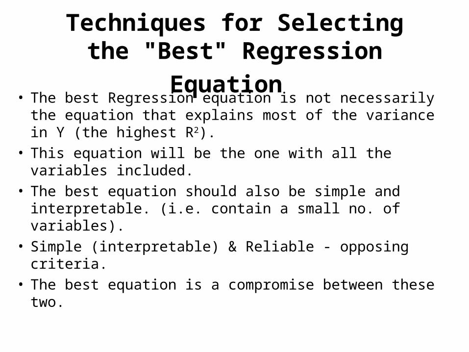
Regression Equation • The best Regression equation is not necessarily the

equation that explains most of the variance in Y (the highest R2).

• This equation will be the one with all the variables included.

• The best equation should also be simple and interpretable. (i.e. contain a small no. of variables).

• Simple (interpretable) & Reliable - opposing criteria.• The best equation is a compromise between these two.

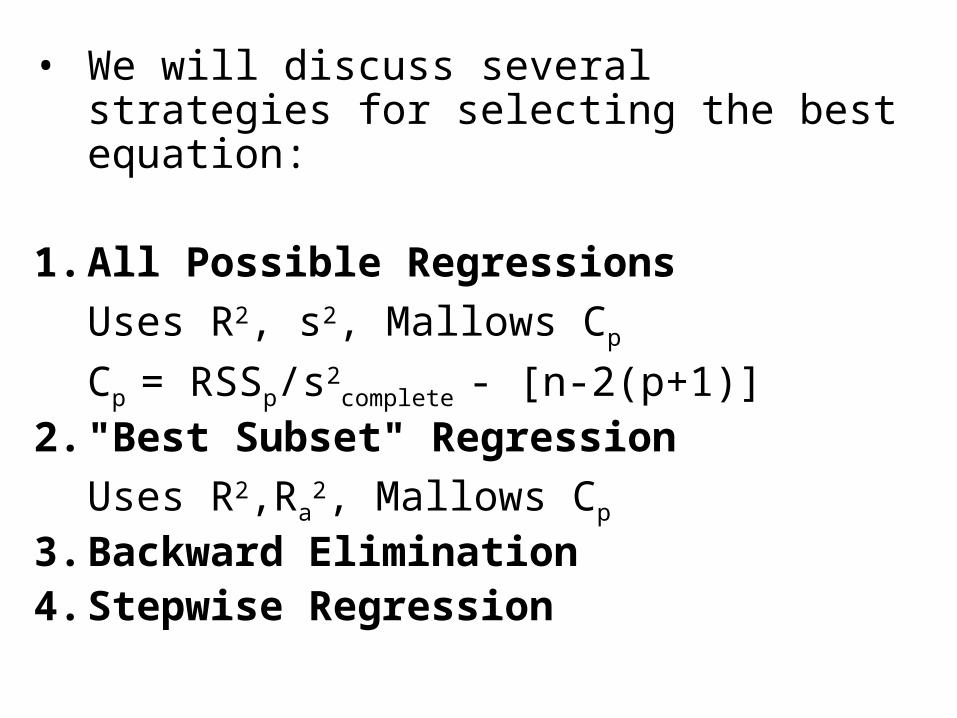
• We will discuss several strategies for selecting the best equation:

 1. All Possible Regressions

Uses R2, s2, Mallows Cp

  Cp = RSSp/s2complete - [n-2(p+1)]

2. "Best Subset" Regression

Uses R2,Ra2, Mallows Cp

3. Backward Elimination4. Stepwise Regression

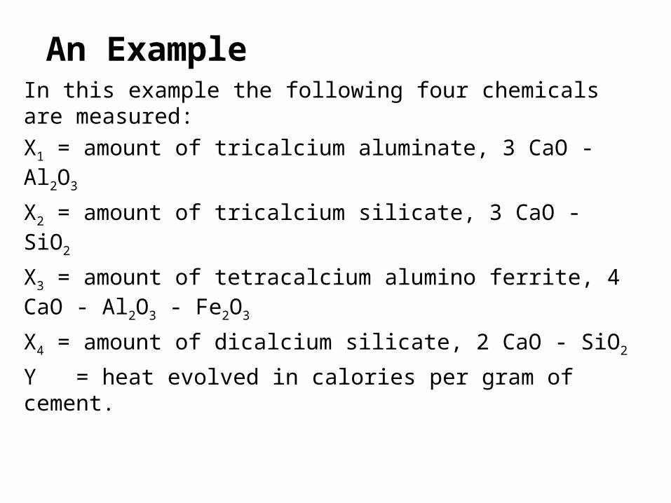
An Example In this example the following four chemicals are measured:

X1 = amount of tricalcium aluminate, 3 CaO - Al2O3

X2 = amount of tricalcium silicate, 3 CaO - SiO2

X3 = amount of tetracalcium alumino ferrite, 4 CaO - Al2O3 - Fe2O3

X4 = amount of dicalcium silicate, 2 CaO - SiO2

Y = heat evolved in calories per gram of cement.

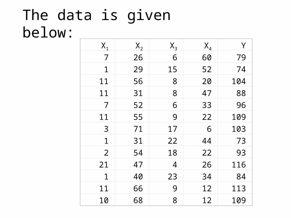
The data is given below:X1 X2 X3 X4 Y

7 26 6 60 79

1 29 15 52 74

11 56 8 20 104

11 31 8 47 88

7 52 6 33 96

11 55 9 22 109

3 71 17 6 103

1 31 22 44 73

2 54 18 22 93

21 47 4 26 116

1 40 23 34 84

11 66 9 12 113

10 68 8 12 109

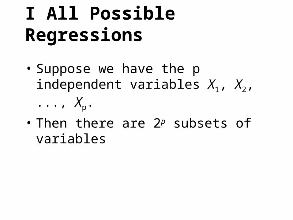
I All Possible Regressions

• Suppose we have the p independent variables X1, X2, ..., Xp.

• Then there are 2p subsets of variables

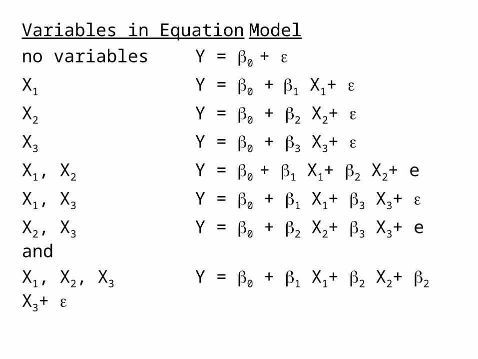
Variables in Equation Model

no variables Y = 0 +

X1 Y = 0 +1 X1+

X2 Y = 0 + 2 X2+

X3 Y = 0 + 3 X3+

X1, X2 Y = 0 + 1 X1+ 2 X2+ e

X1, X3 Y = 0 + 1 X1+ 3 X3+

X2, X3 Y = 0 + 2 X2+ 3 X3+ e and

X1, X2, X3 Y = 0 + 1 X1+ 2 X2+ 2 X3+

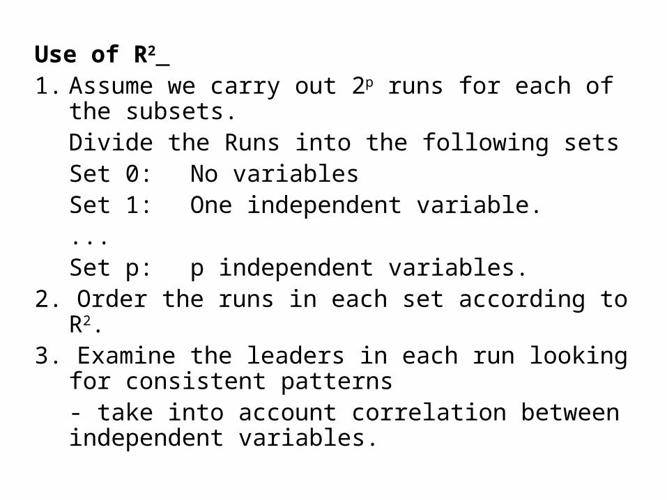
Use of R2 1. Assume we carry out 2p runs for each of the subsets.

Divide the Runs into the following setsSet 0: No variablesSet 1: One independent variable....Set p: p independent variables.

2. Order the runs in each set according to R2.3. Examine the leaders in each run looking for consistent

patterns- take into account correlation between independent variables.

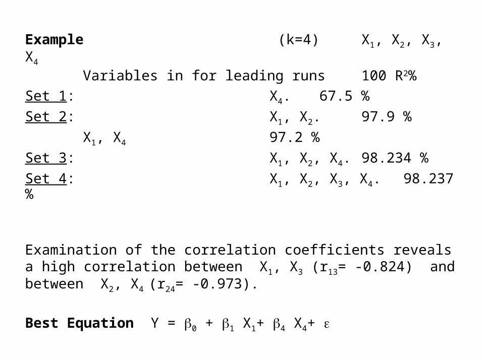
Example (k=4) X1, X2, X3, X4

Variables in for leading runs 100 R2%

Set 1: X4. 67.5 %

Set 2: X1, X2. 97.9 %

X1, X4 97.2 %

Set 3: X1, X2, X4. 98.234 %

Set 4: X1, X2, X3, X4. 98.237 %

 Examination of the correlation coefficients reveals a high correlation between X1, X3 (r13= -0.824) and between X2, X4 (r24= -0.973). 

Best Equation Y = 0 + 1 X1+ 4 X4+

0

10

20

30

40

50

60

70

80

90

0 2 4 6 8 10

p

R2

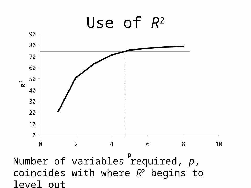
Use of R2

Number of variables required, p, coincides with where R2 begins to level out

Use of the Residual Mean Square (RMS) (s2)• When all of the variables having a non-zero effect

have been included in the mode then the residual mean square is an estimate of s2.

• If "significant" variables have been left out then RMS will be biased upward.

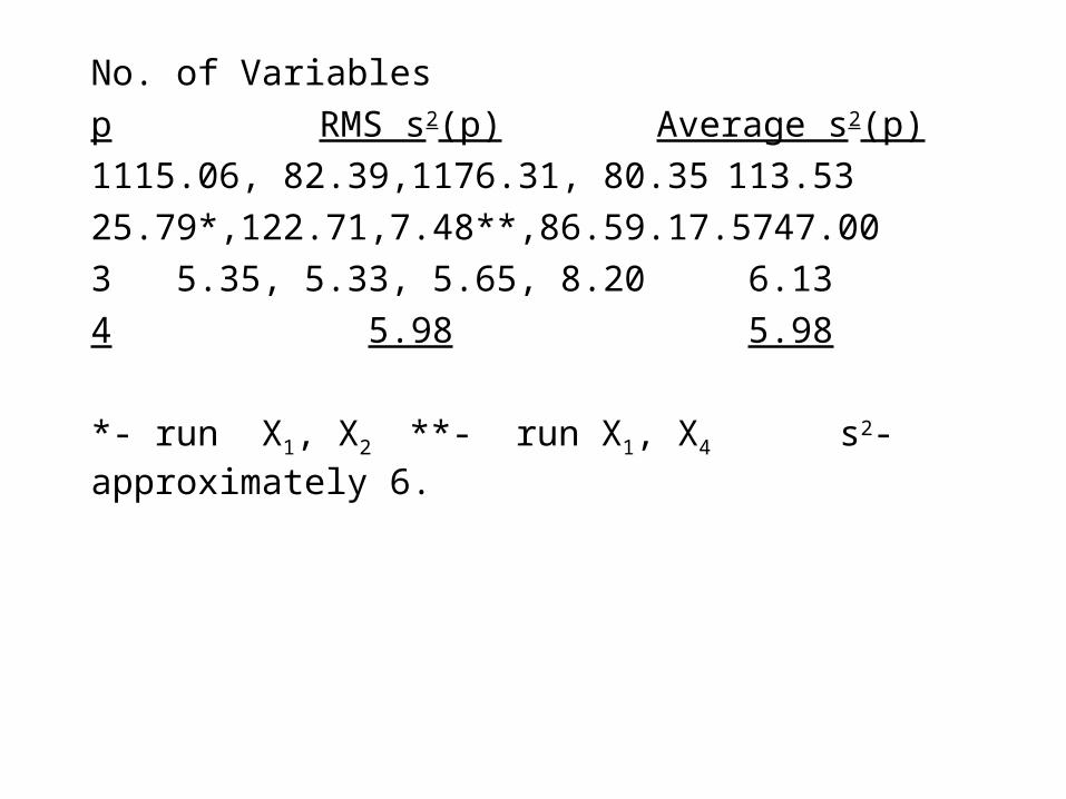
No. of Variables

p RMS s2(p) Average s2(p)

1 115.06, 82.39,1176.31, 80.35 113.53

2 5.79*,122.71,7.48**,86.59.17.57 47.00

3 5.35, 5.33, 5.65, 8.20 6.13

4 5.98 5.98

*- run X1, X2 **- run X1, X4 s2- approximately 6.

0

5

10

15

20

25

0 2 4 6 8 10

p

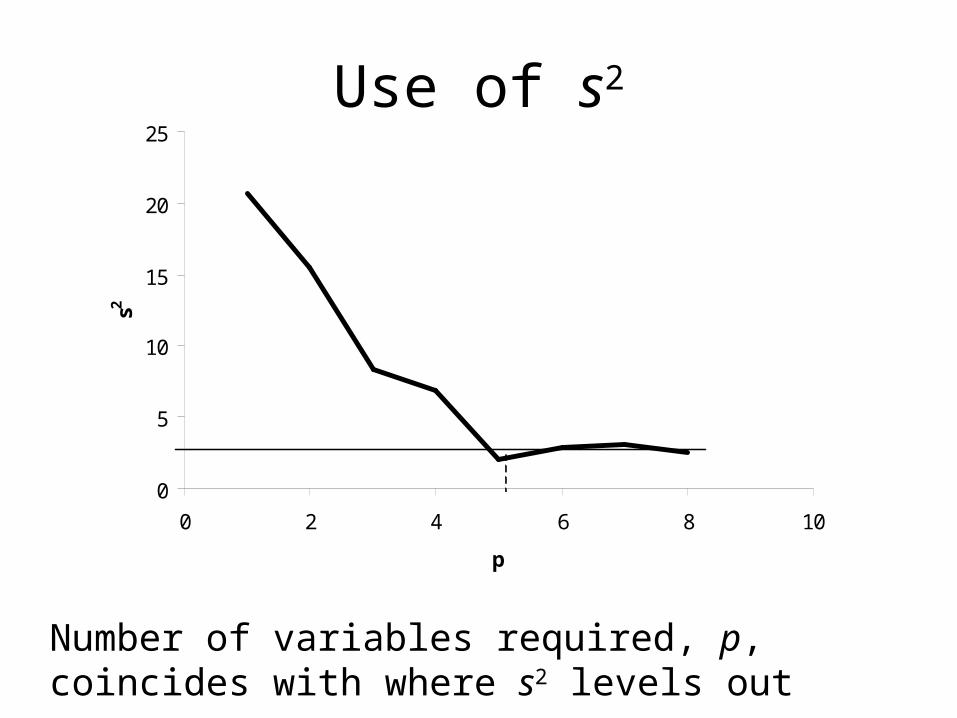
s2Use of s2

Number of variables required, p, coincides with where s2 levels out

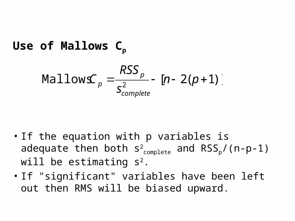
Use of Mallows Cp

• If the equation with p variables is adequate then both s2

complete and RSSp/(n-p-1) will be estimating s2.

• If "significant" variables have been left out then RMS will be biased upward.

)]1(2[ Mallows2

pns

RSSC

complete

pp

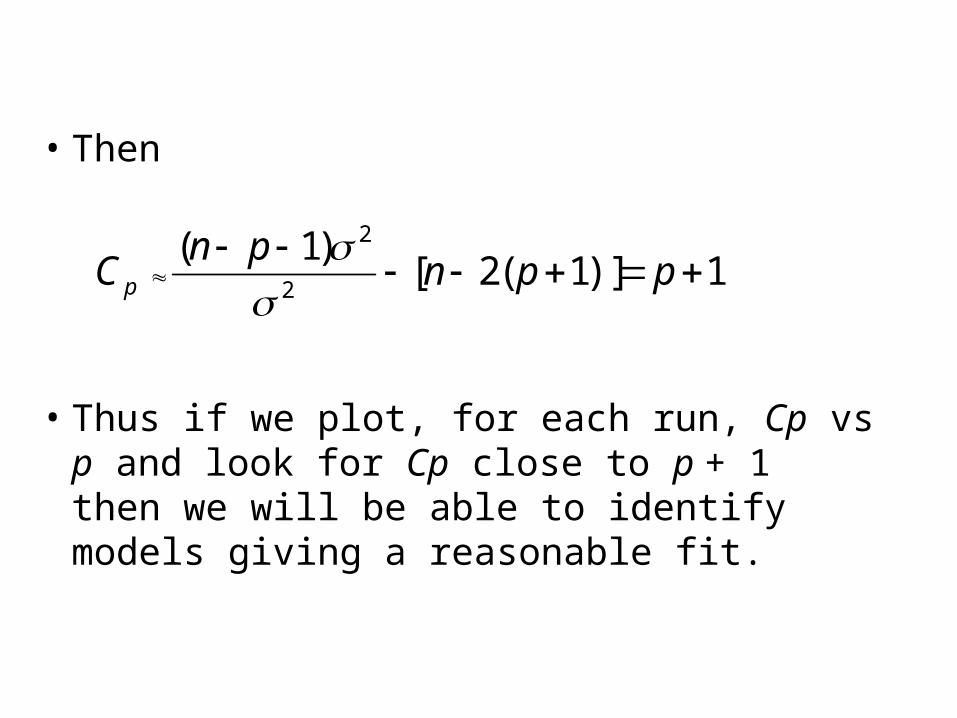
• Then

• Thus if we plot, for each run, Cp vs p and look for Cp close to p + 1 then we will be able to identify models giving a reasonable fit.

1)]1(2[)1(

2

2

ppnpn

C p

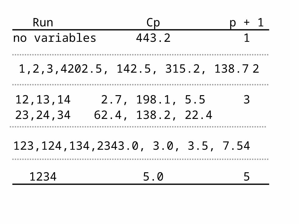
Run Cp p + 1no variables 443.2 1 

1,2,3,4 202.5, 142.5, 315.2, 138.7 2 

12,13,14 2.7, 198.1, 5.5 323,24,34 62.4, 138.2, 22.4

 123,124,134,234 3.0, 3.0, 3.5, 7.5 4 

1234 5.0 5

0

5

10

15

20

0 2 4 6 8 10

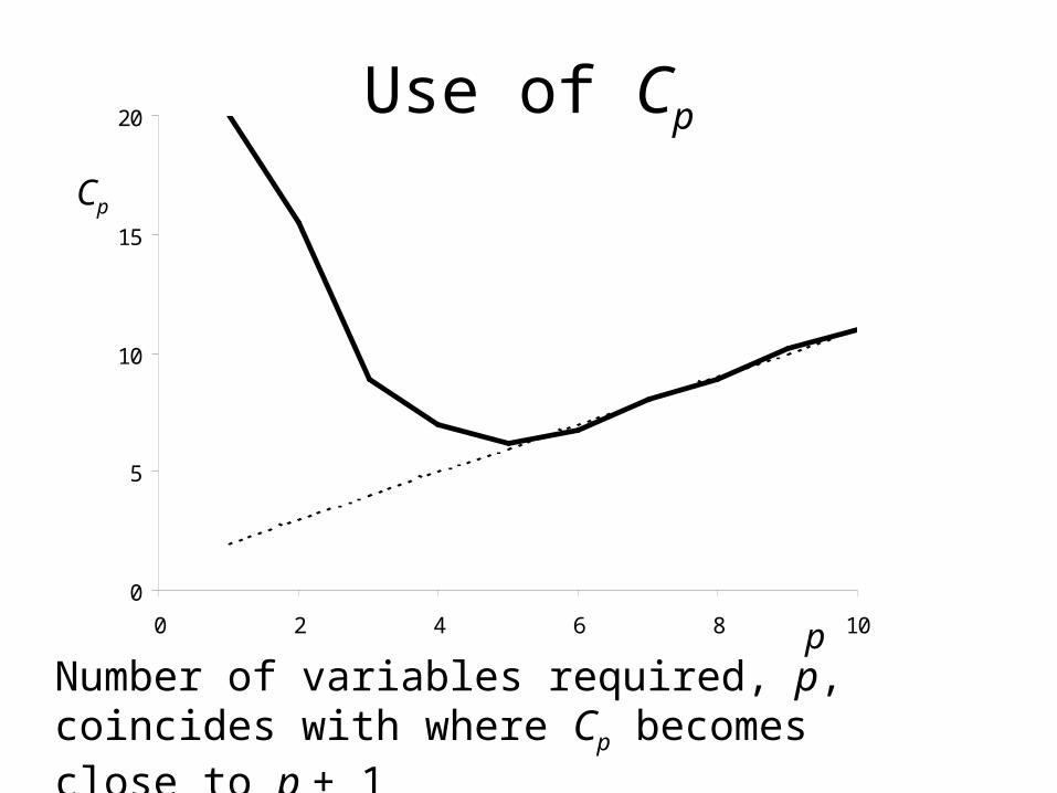
Use of Cp

Number of variables required, p, coincides with where Cp becomes close to p + 1

Cp

p

II "Best Subset" Regression

• Similar to all possible regressions.

• If p, the number of variables, is large then the number of runs , 2p, performed could be extremely large.

• In this algorithm the user supplies the value K and the algorithm identifies the best K subsets of X1, X2, ..., Xp for predicting Y.

III Backward Elimination • In this procedure the complete regression

equation is determined containing all the variables - X1, X2, ..., Xp.

• Then variables are checked one at a time and the least significant is dropped from the model at each stage.

• The procedure is terminated when all of the variables remaining in the equation provide a significant contribution to the prediction of the dependent variable Y.

The precise algorithm proceeds as follows:

1. Fit a regression equation containing all variables in the equation.

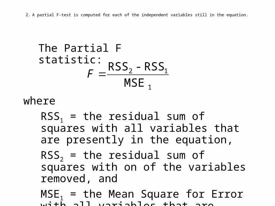
2. A partial F-test is computed for each of the independent variables still in the equation.

 

1

12

MSE

RSS - RSSF

where

RSS1 = the residual sum of squares with all variables that are presently in the equation,

RSS2 = the residual sum of squares with on of the variables removed, and

MSE1 = the Mean Square for Error with all variables that are presently in the equation.

The Partial F statistic:

 

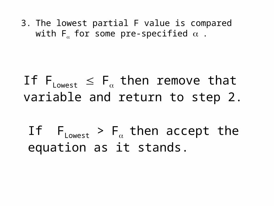
3. The lowest partial F value is compared with Ffor some pre-specified .

If FLowest Fthen remove that variable and return to step 2.

If FLowest > Fthen accept the equation as it stands.

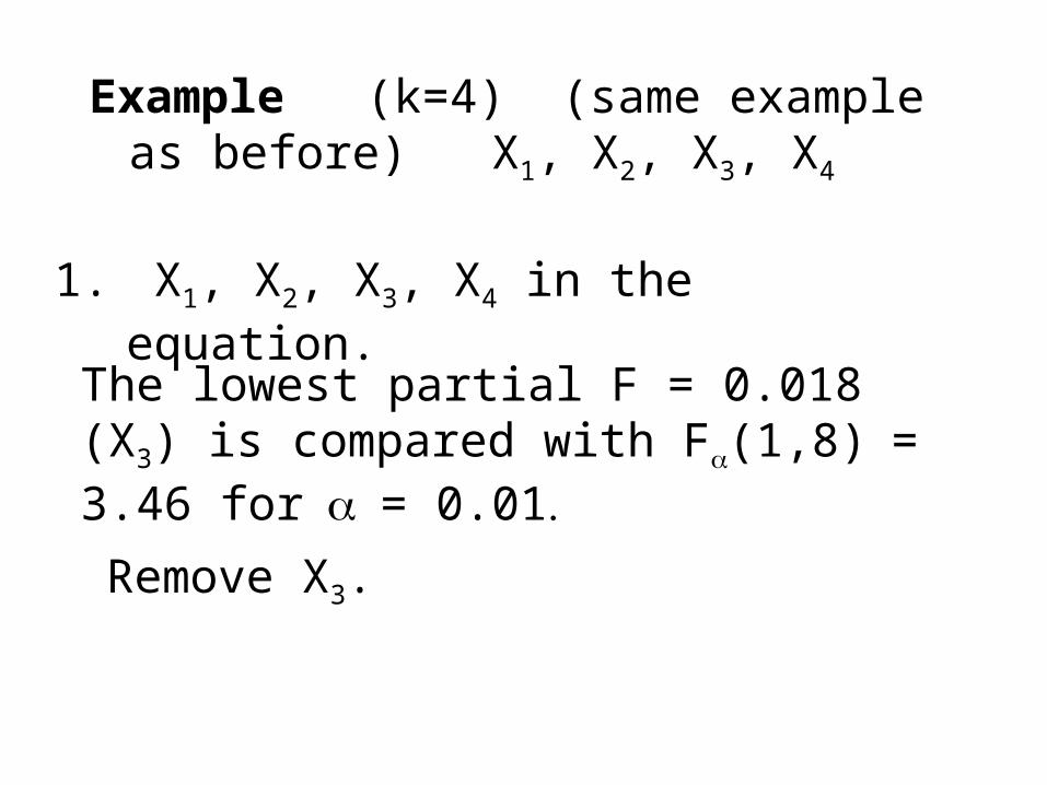
Example (k=4) (same example as before) X1, X2, X3, X4

1. X1, X2, X3, X4 in the equation.

The lowest partial F = 0.018 (X3) is compared with F(1,8)= 3.46 for= 0.01

Remove X3.

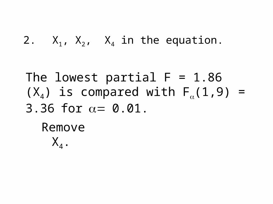
2. X1, X2, X4 in the equation.

The lowest partial F = 1.86 (X4) is compared with F(1,9) = 3.36for0.01.

Remove X4.

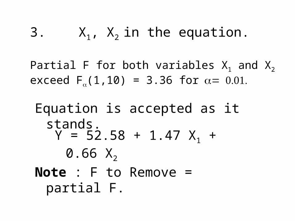
Partial F for both variables X1 and X2 exceed F(1,10) = 3.36 for

3. X1, X2 in the equation.

Equation is accepted as it stands.

Y = 52.58 + 1.47 X1 + 0.66 X2

Note : F to Remove = partial F.

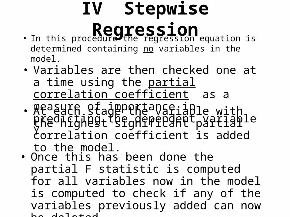
IV Stepwise Regression• In this procedure the regression equation is

determined containing no variables in the model.

• Variables are then checked one at a time using the partial correlation coefficient as a measure of importance in predicting the dependent variable Y.

• At each stage the variable with the highest significant partial correlation coefficient is added to the model.

• Once this has been done the partial F statistic is computed for all variables now in the model is computed to check if any of the variables previously added can now be deleted.

• This procedure is continued until no further variables can be added or deleted from the model.

• The partial correlation coefficient for a given variable is the correlation between the given variable and the response when the present independent variables in the equation are held fixed.

• It is also the correlation between the given variable and the residuals computed from fitting an equation with the present independent variables in the equation.

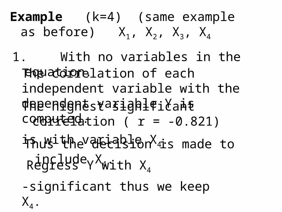
Example (k=4) (same example as before) X1, X2, X3, X4

1. With no variables in the equation. The correlation of each independent variable with the dependent variable Y is computed.

The highest significant correlation ( r = -0.821)

is with variable X4.

Thus the decision is made to include X4.

Regress Y with X4

-significant thus we keep X4.

2. Compute partial correlation coefficients of Y with all other independent variables given X4 in the equation.

The highest partial correlation is with the variable X1. ( [rY1.4]2 = 0.915).

Thus the decision is made to include X1.

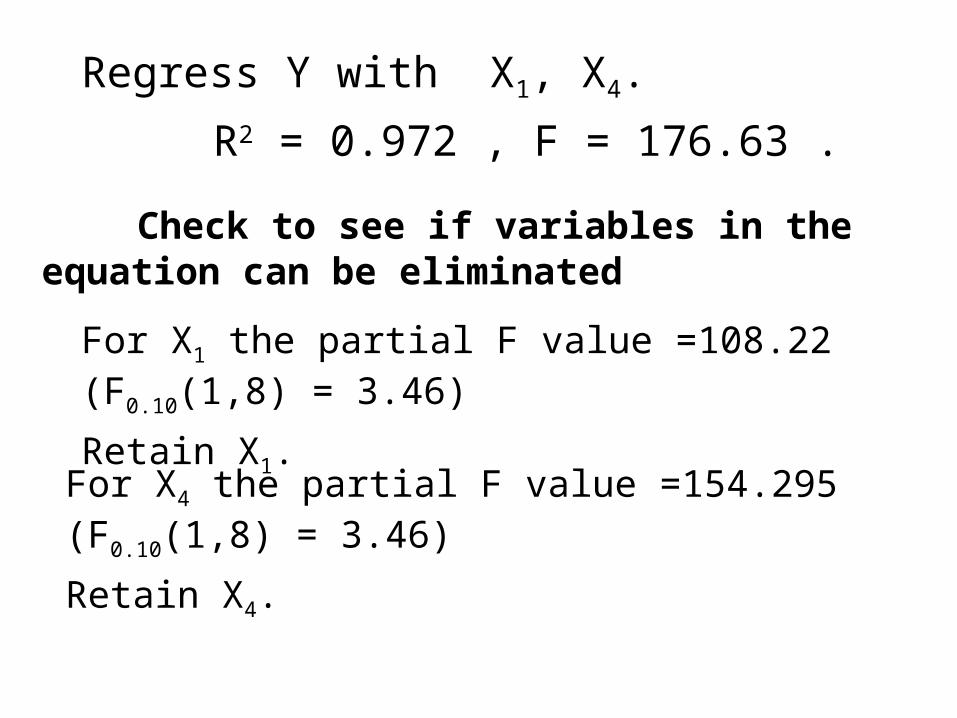
Regress Y with X1, X4.

R2 = 0.972 , F = 176.63 .

 

For X1 the partial F value =108.22 (F0.10(1,8) = 3.46)

Retain X1.

For X4 the partial F value =154.295 (F0.10(1,8) = 3.46)

Retain X4.

Check to see if variables in the equation can be eliminated

 

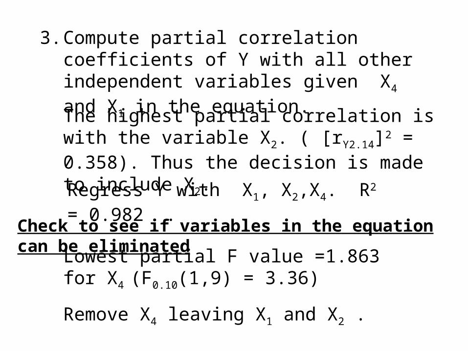
3. Compute partial correlation coefficients of Y with all other independent variables given X4 and X1 in the equation.

The highest partial correlation is with the variable X2. ( [rY2.14]2 = 0.358). Thus the decision is made to include X2.

Regress Y with X1, X2,X4. R2 = 0.982 .

Lowest partial F value =1.863 for X4

(F0.10(1,9) = 3.36)

Remove X4 leaving X1 and X2 .

Check to see if variables in the equation can be eliminated

Examples

Using Statistical Packages