Embed Size (px)
Citation preview
Psicologica (2004), 25, 253-274
Structural Equation Modelling ofMultiple Facet Data: Extending Models
for Multitrait-Multimethod Data
Timo M. Bechger and Gunter MarisCITO (The Netherlands)
AbstractThis paper is about the structural equation modelling of quantitative mea-sures that are obtained from a multiple facet design. A facet is simply a setconsisting of a finite number of elements. It is assumed that measures areobtained by combining each element of each facet. Methods and traits aretwo such facets, and a multitrait-multimethod study is a two-facet design.We extend models that were proposed for multitrait-multimethod data byWothke (1984;1996) and Browne (1984, 1989, 1993), and demonstrate howthey can be fitted using standard software for structural equation modelling.Each model is derived from the model for individual measurements in orderto clarify the first principles underlying each model.
Introduction
A Multi-Trait Multi-Method (MTMM)study is characterized by mea-
sures that are composed as combinations of traits and methods. In this paper,
we will treat a more general case where measures are composed as combi-
nations of elements of facets. Afacet is simply a set consisting of a finite
Address correspondence to: Timo Bechger, CITO, P.O. Box 1034, NL-6801 MG, Arn-hem, The Netherlands. E-mail: [email protected]; Tel:+31-026-3521162.
254 T.M. Bechger and G. Maris
number of elements, usually calledconditions. Facets refer to properties of
the measures or measurement conditions. Methods and traits are two such
facets, and a MTMM study is a (fully crossed) two-facet design. Facets need
not be methods or traits or anything in particular. Consider, for example, a
study that is presented by Browne (1970) and discussed in detail by Joreskog
and Sorbom (1996, section6.3). Persons were seated in a darkened room
and required to place a rod in vertical position by pushing buttons. The score
was the (positive or negative) angle of the rod from the vertical. Each person
had to perform the task twice in a number of different situations which where
constructed according to a two-facet design. The two facets were the posi-
tion of the chair and the initial position of the rod, each with three conditions.
The occasion of the experiment may be considered the third facet with two
conditions.
We assume that measures were constructed for each combination of the
facets and that we have data for each measure. We further assume that mea-
sures are continuous. We believe that the case of discrete data is more appro-
priately handled using item response theory models (e.g., Bechger, Verhelst
& Verstralen, 2001).
To analyze data from a multiple facet design, we extend two models
that were suggested for the MTMM design: thecovariance component model
(Wothke, 1984, 1996), and thecomposite direct product model(Browne,
1984, 1989, 1993). In doing so, we pursue e.g., Bagozzi, Yi and Nassen,
(1999), Cudeck (1988), or Browne and Strydom (1997) who suggest general-
ization of the composite direct product model to multiple facets. Our objective
is to demonstrate how researchers who know the basic principles ofstructural
equation modelling(SEM) may formulate and fit these models using the LIS-
REL (Joreskog & Sorbom, 1996) or the Mx program1 (Neale, Boker, Xie, &
Maes, 2002). There are several alternative software packages but the major-
ity of these have an interface that is similar to that of LISREL or Mx. For a
general introduction to SEM we refer the reader to Bollen (1989).
1The Mx program is free-ware and can, at present, be obtained from the internet addresshttp://www.vcu.edu/mx/index.html
Structural Equation Modelling of Multiple Facet Data 255
Each model is derived from the (data) model for individual measure-
ments in order to clarify the first principles underlying each model. In the con-
text of MTMM studies, the model for the observations is of less interest since
the main objective is to establish a structure for the correlations that relates
to the Campbell and Fiske (1959) criteria for convergent and discriminant va-
lidity. However, in general multi-facet studies the data model is important as
a substantive hypothesis that guides the interpretation of the parameters. We
demonstrate how each of the models can be fitted to a correlation or covari-
ance matrix. (We refer to Cudeck (1989) for a survey of the issues concerning
the analysis of correlation matrices). As an illustration, we discuss a number
of applications to real data.
Preliminaries
Persons (or, more general,objects) are assumed to be drawnat random
from a large population and each observation is taken to be a realization of
a random vectorx of measurements made under combinations of conditions
of multiple facets. All models that are considered here are based upon the
following linear model for the observations
x = µ + η + u ,
whereµ denote the mean ofx, and the latent variableη represents true or
common scores. The components ofu represent measurement error and are
assumed to be uncorrelated with mean zero and variance matrixDu. The
common scores are uncorrelated tou; they have zero mean and covariance
matrixΣη. It follows that the data have mean vectorµ and covariance matrix
Σ = Ση + Du ,
whereDu is a diagonal matrix.
We use the following notation: In a design with multiple facets, A, B,
C, D, etc. denote the facets. Each facet has several conditions (or elements)
denoted by Ai, Bj, etc. The number of conditions in each facet is denoted
256 T.M. Bechger and G. Maris
by the lowercase of the letter that is used to denote the facet. For example,
a = 3 if facet A has three conditions. We useF to denote a generic facet. The
number of measures that can be constructed (e.g.,a× b× c if there are three
facets) will be denoted byp. The number of facets will be denoted by #F. The
sum of the conditions in each of the facets (e.g.,a + b + c) will be denoted
by #f. The symbolIa denotes an identity matrix of dimensiona and1a a
unit vector witha elements. The symbol⊗ denotes the Kronecker or direct
product operator withA⊗B = (aijB). Finally, the vectorzF denotes a vector
of random variables associated with a facet; that is,zF = (z(F1), . . ., z(Ff ))T ,
wherez(Fj) denotes a random variable associated with the j-th condition of
facet F. UppercaseT refers to transposition.
The Covariance Component Model
Wothke (1984) suggested that theCovariance Component(CC) model
described by Bock and Bargmann (1966) be used for MTMM data. In this
section, we discuss a number of parameterizations of the CC model and
demonstrate how each is specified within the LISREL framework. Note that
the CC model is related to random effects analysis of variance (see Bock &
Bargmann, 1966, pp. 508-509) but we will not explicitly use this relationship
in our presentation of the model.
Introduction
Let ηx denote a generic element ofη; i.e., x is a measurement obtained
as the combination ofAi, Bj, . . . , Er. In the CC model,η is assumed to have
an additive structure. Specifically,
ηx = g + z(Ai) + z(Bj) + . . . + z(Er) ,
whereg denotes a within-person mean. In matrix notation:
η = Az ,
wherez =(g, zT
A, zTB, . . . , zT
E
)T, andA is ap × (1 + #f) incidence matrix;
that is, a matrix whose entries are zero or one. The rows ofA indicate all
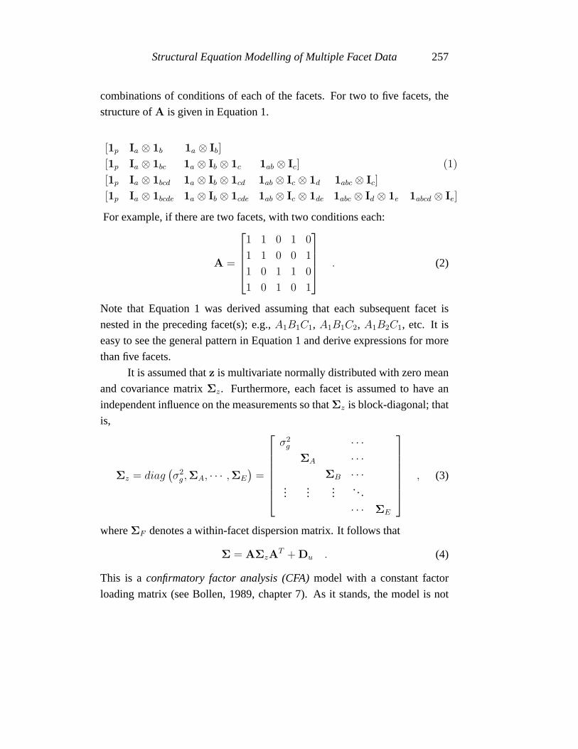
Structural Equation Modelling of Multiple Facet Data 257
combinations of conditions of each of the facets. For two to five facets, the
structure ofA is given in Equation 1.
[1p Ia ⊗ 1b 1a ⊗ Ib]
[1p Ia ⊗ 1bc 1a ⊗ Ib ⊗ 1c 1ab ⊗ Ic] (1)
[1p Ia ⊗ 1bcd 1a ⊗ Ib ⊗ 1cd 1ab ⊗ Ic ⊗ 1d 1abc ⊗ Ic]
[1p Ia ⊗ 1bcde 1a ⊗ Ib ⊗ 1cde 1ab ⊗ Ic ⊗ 1de 1abc ⊗ Id ⊗ 1e 1abcd ⊗ Ie]
For example, if there are two facets, with two conditions each:
A =
1 1 0 1 0
1 1 0 0 1
1 0 1 1 0
1 0 1 0 1
. (2)
Note that Equation 1 was derived assuming that each subsequent facet is
nested in the preceding facet(s); e.g.,A1B1C1, A1B1C2, A1B2C1, etc. It is
easy to see the general pattern in Equation 1 and derive expressions for more
than five facets.
It is assumed thatz is multivariate normally distributed with zero mean
and covariance matrixΣz. Furthermore, each facet is assumed to have an
independent influence on the measurements so thatΣz is block-diagonal; that
is,
Σz = diag(σ2
g ,ΣA, · · · ,ΣE
)=
σ2
g · · ·ΣA · · ·
ΣB · · ·...
......
...
· · · ΣE
, (3)
whereΣF denotes a within-facet dispersion matrix. It follows that
Σ = AΣzAT + Du . (4)
This is aconfirmatory factor analysis (CFA)model with a constant factor
loading matrix (see Bollen, 1989, chapter 7). As it stands, the model is not
258 T.M. Bechger and G. Maris
identifiable. Informally, this means that no amount of data will help to deter-
mine the true value of one or more of the parameters. We will demonstrate
this by constructing an equivalent model with less parameters.
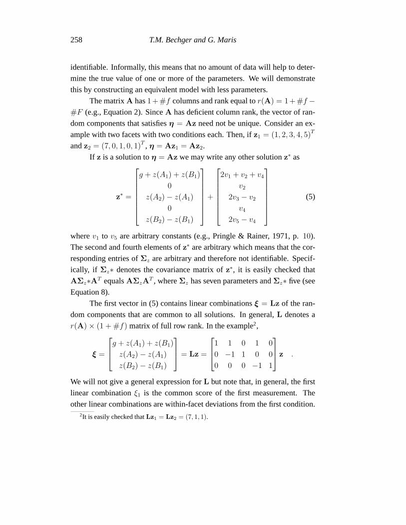
The matrixA has1+#f columns and rank equal tor(A) = 1+#f −#F (e.g., Equation 2). SinceA has deficient column rank, the vector of ran-
dom components that satisfiesη = Az need not be unique. Consider an ex-
ample with two facets with two conditions each. Then, ifz1 = (1, 2, 3, 4, 5)T
andz2 = (7, 0, 1, 0, 1)T , η = Az1 = Az2.
If z is a solution toη = Az we may write any other solutionz∗ as
z∗ =
g + z(A1) + z(B1)
0
z(A2)− z(A1)
0
z(B2)− z(B1)
+
2v1 + v2 + v4
v2
2v3 − v2
v4
2v5 − v4
(5)
wherev1 to v5 are arbitrary constants (e.g., Pringle & Rainer, 1971, p.10).
The second and fourth elements ofz∗ are arbitrary which means that the cor-
responding entries ofΣz are arbitrary and therefore not identifiable. Specif-
ically, if Σz∗ denotes the covariance matrix ofz∗, it is easily checked that
AΣz∗AT equalsAΣzAT , whereΣz has seven parameters andΣz∗ five (see
Equation 8).
The first vector in (5) contains linear combinationsξ = Lz of the ran-
dom components that are common to all solutions. In general,L denotes a
r(A)× (1 + #f) matrix of full row rank. In the example2,
ξ =
g + z(A1) + z(B1)
z(A2)− z(A1)
z(B2)− z(B1)
= Lz =
1 1 0 1 0
0 −1 1 0 0
0 0 0 −1 1
z .
We will not give a general expression forL but note that, in general, the first
linear combinationξ1 is the common score of the first measurement. The
other linear combinations are within-facet deviations from the first condition.2It is easily checked thatLz1 = Lz2 = (7, 1, 1).
Structural Equation Modelling of Multiple Facet Data 259
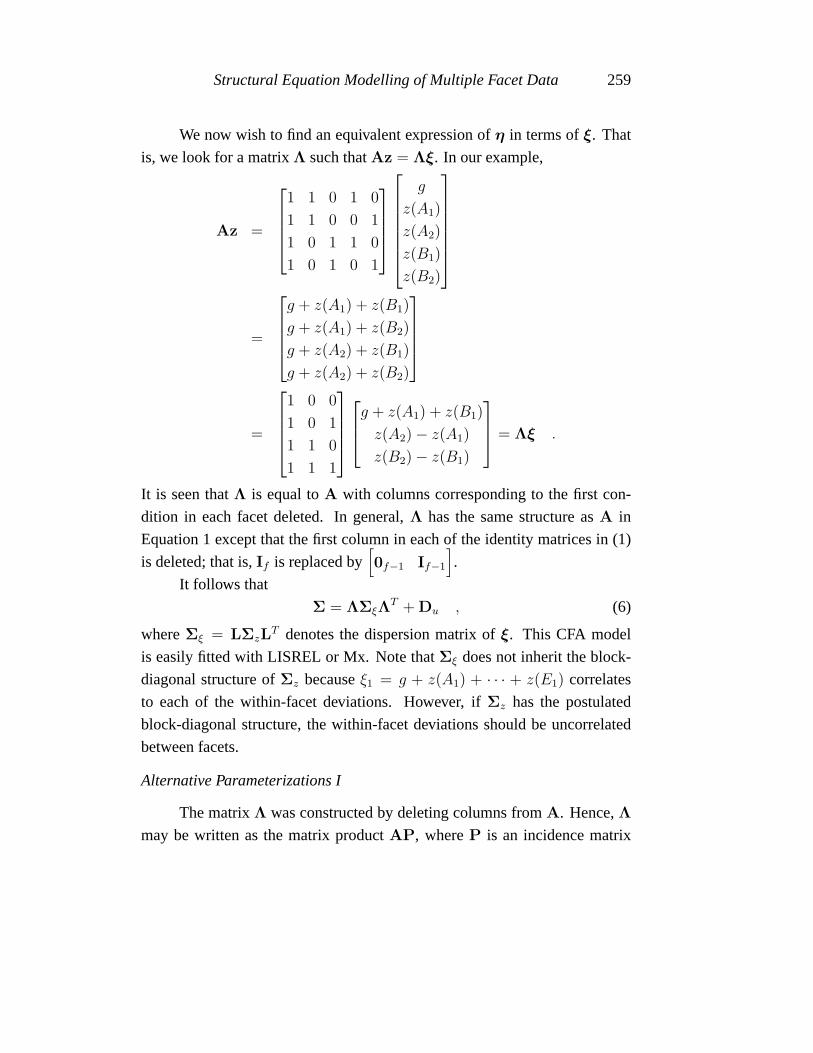
We now wish to find an equivalent expression ofη in terms ofξ. That
is, we look for a matrixΛ such thatAz = Λξ. In our example,
Az =
1 1 0 1 0
1 1 0 0 1
1 0 1 1 0
1 0 1 0 1
g
z(A1)
z(A2)
z(B1)
z(B2)
=
g + z(A1) + z(B1)
g + z(A1) + z(B2)
g + z(A2) + z(B1)
g + z(A2) + z(B2)
=
1 0 0
1 0 1
1 1 0
1 1 1
g + z(A1) + z(B1)
z(A2)− z(A1)
z(B2)− z(B1)
= Λξ .
It is seen thatΛ is equal toA with columns corresponding to the first con-
dition in each facet deleted. In general,Λ has the same structure asA in
Equation 1 except that the first column in each of the identity matrices in (1)
is deleted; that is,If is replaced by[0f−1 If−1
].
It follows that
Σ = ΛΣξΛT + Du , (6)
whereΣξ = LΣzLT denotes the dispersion matrix ofξ. This CFA model
is easily fitted with LISREL or Mx. Note thatΣξ does not inherit the block-
diagonal structure ofΣz becauseξ1 = g + z(A1) + · · · + z(E1) correlates
to each of the within-facet deviations. However, ifΣz has the postulated
block-diagonal structure, the within-facet deviations should be uncorrelated
between facets.
Alternative Parameterizations I
The matrixΛ was constructed by deleting columns fromA. Hence,Λ
may be written as the matrix productAP, whereP is an incidence matrix
260 T.M. Bechger and G. Maris
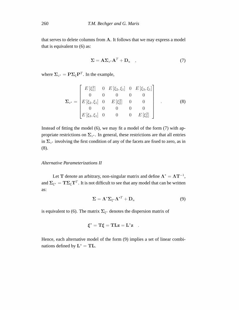
that serves to delete columns fromA. It follows that we may express a model
that is equivalent to (6) as:
Σ = AΣz∗AT + Du , (7)
whereΣz∗ = PΣξPT . In the example,
Σz∗ =
E [ξ2
1 ] 0 E [ξ2, ξ1] 0 E [ξ3, ξ1]
0 0 0 0 0
E [ξ2, ξ1] 0 E [ξ22 ] 0 0
0 0 0 0 0
E [ξ3, ξ1] 0 0 0 E [ξ23 ]
. (8)
Instead of fitting the model (6), we may fit a model of the form (7) with ap-
propriate restrictions onΣz∗. In general, these restrictions are that all entries
in Σz∗ involving the first condition of any of the facets are fixed to zero, as in
(8).
Alternative Parameterizations II
Let T denote an arbitrary, non-singular matrix and defineΛ∗ = ΛT−1,
andΣξ∗ = TΣξTT . It is not difficult to see that any model that can be written
as:
Σ = Λ∗Σξ∗Λ∗T + Du (9)
is equivalent to (6). The matrixΣξ∗ denotes the dispersion matrix of
ξ∗ = Tξ = TLz = L∗z .
Hence, each alternative model of the form (9) implies a set of linear combi-
nations defined byL∗ = TL.
Structural Equation Modelling of Multiple Facet Data 261
Browne (1989) considers linear combinations of the form:
ξ∗ = L∗z =
1 12
12
12
12
0 −12
12
0 0
0 0 0 −12
12
g
z(A1)
z(A2)
z(B1)
z(B2)
=
g + 12(z(A1) + z(A2)) + 1
2(z(B1) + z(B2))
12(z(A2)− z(A1))
12(z(B2)− z(B1))
.
The corresponding matrixT, is found be solvingL∗ = TL. Here,
L∗ =
1 12
12
12
12
0 −12
12
0 0
0 0 0 −12
12
= TL =
1 12
12
0 12
0
0 0 12
1 1 0 1 0
0 −1 1 0 0
0 0 0 −1 1
.
The correspondingΛ∗ is
Λ∗ =
1 −1 −1
1 −1 1
1 1 −1
1 1 1
= ΛT−1 =
1 0 0
1 0 1
1 1 0
1 1 1
1 −1 −1
0 2 0
0 0 2
.
For later reference, we call this parametrizationBrowne’s parametrization. In
general, if we use Browne’s parametrization,Λ∗ has the same structure asA
in Equation 1, except that each of the identity matricesIf in (1) is replaced
by the matrix[−1f−1 If−1
]T
. There is, of course, an infinite number of
alternative parameterizations, each corresponding to a non-singular matrixT
and a matrixL∗ (see e.g., Bock & Bargmann, 1966, table 6).
Browne (1989) implicitly assumes that sub-matricesΣF in (3) have
equal diagonal elements. This implies thatΣξ∗ = L∗ΣzL∗T is block-
diagonal. For instance,
E [ξ∗1 , ξ∗2 ] = E
[1
2(z(A1) + z(A2)) ,
1
2(z(A2)− z(A1))
]=
1
4
(σ2
z(A2) − σ2z(A1)
),
262 T.M. Bechger and G. Maris
which is zero if and only ifσ2z(A1) = σ2
z(A2).
Fitting the Covariance Component model to a Correlation Matrix
To fit the model to a correlation matrix we need to derive the model
for the correlation matrixP = DxΣDx, whereDx = diag−12 (Σ); a diagonal
matrix with on the diagonal the inverses of the population standard-deviations
of the observed measures. That is,
P = Dx (Ση + Du)Dx = Dx
(ΛΣξΛ
T + Du
)Dx . (10)
This model is easily fitted with LISREL. One may, as in (10), use our first
parametrization and specify: ny = ne = p, nk= r (A), PSI= 0, LAMBDA-Y
= Dx, GAMMA = Λ, and PHI= Σξ. An example of a LISREL script is
provided in the Appendix. Only small changes are necessary to specifyΣη
as in (7) or (9). Note that (10) is a special case of the scale-free covariance
model proposed by Wiley, Schmidt, and Bramble (1973).
There is a caveat however. Wothke (1988; 1996) claims that the vari-
ance ofξ1 and covariances involvingξ1 are not identifiable. Hence, in general,
model (10) is unsuited for correlation matrices. As mentioned before, Browne
(1989) assumes that the within-facet dispersion matrices have equal diagonal
elements. Suppose that this assumption holds. Then, if Browne’s parametriza-
tion is used, and the matrixΣη in (10) is specified asΛ∗Σξ∗Λ∗T , the matrix
Σξ∗ is block-diagonal and the model may be used for correlation matrices
provided the variance ofξ∗1 is known. Browne (1989) sets the variance of
ξ∗1 to one. This means that all variances and covariance must be interpreted
relative to the variance ofξ∗1 .
Applications of the Covariance ComponentModel
To a Covariance Matrix
For illustration we apply the CC model to three-facet data gathered by
Hilton, Beaton, and Bower (1971). The data consist of2163 measurements of
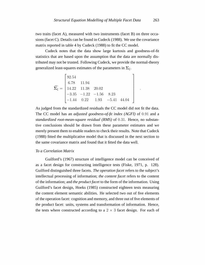
Structural Equation Modelling of Multiple Facet Data 263
two traits (facet A), measured with two instruments (facet B) on three occa-
sions (facet C). Details can be found in Cudeck (1988). We use the covariance
matrix reported in table 4 by Cudeck (1988) to fit the CC model.
Cudeck notes that the data show large kurtosis and goodness-of-fit
statistics that are based upon the assumption that the data are normally dis-
tributed may not be trusted. Following Cudeck, we provide the normal-theory
generalized least-squares estimates of the parameters inΣξ.
Σξ =
92.54
6.78 11.94
14.22 11.38 20.02
−3.35 −1.22 −1.56 8.23
−1.44 0.22 1.93 −5.41 44.04
.
As judged from the standardized residuals the CC model did not fit the data.
The CC model has anadjusted goodness-of-fit index (AGFI)of 0.91 and a
standardized root-mean-square residual (RMS)of 0.31. Hence, no substan-
tive conclusions should be drawn from these parameter estimates and we
merely present them to enable readers to check their results. Note that Cudeck
(1988) fitted the multiplicative model that is discussed in the next section to
the same covariance matrix and found that it fitted the data well.
To a Correlation Matrix
Guilford’s (1967) structure of intelligence model can be conceived of
as a facet design for constructing intelligence tests (Fiske, 1971, p. 128).
Guilford distinguished three facets.The operation facetrefers to the subject’s
intellectual processing of information;the content facetrefers to the content
of the information; andthe product facetto the form of the information. Using
Guilford’s facet design, Hoeks (1985) constructed eighteen tests measuring
the content element semantic abilities. He selected two out of five elements
of the operation facet: cognition and memory, and three out of five elements of
the product facet: units, systems and transformation of information. Hence,
the tests where constructed according to a2 × 3 facet design. For each of
264 T.M. Bechger and G. Maris
the combinations, Hoeks constructed three different tests. The tests may be
considered as a third facet and we treat the measures as arising from a2×3×3
facet design. The data were analyzed earlier using a standard confirmatory
factor model by Hoeks, Mellenbergh and Molenaar (1989). We fit the CC
model to the correlation matrix that they give in their report (see Appendix).
Following Hoeks, Mellenbergh, and Molenaar (1989) we used un-
weighted least-squares to fit model (10) to the correlation matrix, assuming
a block-diagonal structure forΣξ∗. The CC model reproduced the observed
correlation matrix well as judged from the residuals. Deviations correspond-
ing to the third facet (different tests) showed zero variation relative to the
combination of the first condition in each facet. Thus, we specified a model
for two facets with three measures for each combination and found a model
that fitted equally satisfactorily. This model is easily specified by deleting
the columns of the third facet from theA matrix. Finally, we found that we
could specifyΣξ∗ as a diagonal matrix without visible deterioration of the fit.
The final model has an AGFI of0.99, and a RMS of0.051, comparable to the
values found by Hoeks, et al. (1989). Other fit indices are not reported be-
cause they require normal distributions. A LISREL script for the final model
is in the Appendix. Our analysis suggests that the facet-structure suggested
by Guilford does indeed hold.
The Composite Direct Product Model
The multiplicative data model may be derived from the following mul-
tiplicative structure for the common scoreη:
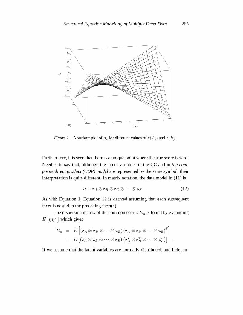
ηx = z(Aj)z(Bk) · · · z(Er) . (11)
In contrast to the CC model, it is now assumed that the true score is the
product of a set of latent variables. It is clear that (11) represents a strong
hypothesis; one that will not often be deemed realistic in social science ap-
plications. As illustrated in Figure 1 for two facets, different values ofz(Ai)
give the same true score in combination with two different values ofz(Bj).
Structural Equation Modelling of Multiple Facet Data 265
−100
−80
−60
−40
−20
0
20
40
60
80
100
z(Ai)
z(Bj)
η x
Figure 1. A surface plot ofηx for different values ofz(Ai) andz(Bj)
Furthermore, it is seen that there is a unique point where the true score is zero.
Needles to say that, although the latent variables in the CC and inthe com-
posite direct product (CDP) modelare represented by the same symbol, their
interpretation is quite different. In matrix notation, the data model in (11) is
η = zA ⊗ zB ⊗ zC ⊗ · · · ⊗ zE . (12)
As with Equation 1, Equation 12 is derived assuming that each subsequent
facet is nested in the preceding facet(s).
The dispersion matrix of the common scoresΣη is found by expanding
E[ηηT
]which gives
Ση = E[(zA ⊗ zB ⊗ · · · ⊗ zE) (zA ⊗ zB ⊗ · · · ⊗ zE)T
]= E
[(zA ⊗ zB ⊗ · · · ⊗ zE)
(zT
A ⊗ zTB ⊗ · · · ⊗ zT
E
)].
If we assume that the latent variables are normally distributed, and indepen-
266 T.M. Bechger and G. Maris
dent between facets,Ση has a multiplicative structure; that is,
Ση = E[zAzT
A ⊗ zBzTB ⊗ · · · zEzT
E
]= ΣA ⊗ΣB ⊗ · · · ⊗ΣE .
It follows that
Σ = ΣA ⊗ΣB ⊗ · · · ⊗ΣE + Du . (13)
Note that the common scores are not normally distributed under this model
since the product of normally distributed variables is not normally distributed.
There is an equivalent specification of the model with standardized
within-facet dispersion matrices. The true score dispersion matrix is stan-
dardized by pre- and post-multiplying the dispersion matrices by a diagonal
matrixDη = diag−12 [Ση] that contains the inverse of the true score standard
deviations. The multiplicative structure ofΣη implies that this matrix is found
to be structured as follows:
Dη = DA ⊗DB ⊗ · · · ⊗DE ,
whereDF = diag−12 (ΣF ). Hence, the correlation matrix of the common
scores,Pη, is
Pη = DηΣηDη
= (DAΣADA)⊗ (DBΣBDB)⊗ · · · ⊗ (DEΣEDE)
= PA ⊗PB · · · ⊗PE .
The symmetric matricesPF are thewithin-facet correlation matricesunder
the CDP model. It follows that
Σ = D−1η (Pη + DηDuDη)D
−1η = D−1
η (Pη + D∗U)D−1
η . (14)
The elements of thep × p diagonal matrixD∗U represent ratios of unique
variance to common score variance and one minus any diagonal element of
D∗U equals the classical test theory reliability of the corresponding measure.
The matrixD−1η has a multiplicative structure since
D−1η = (DA ⊗DB ⊗ · · · ⊗DE)−1 = D−1
A ⊗D−1B ⊗ · · · ⊗D−1
E .

Structural Equation Modelling of Multiple Facet Data 267
The model in (14) has the same form as (10) and may be fitted using
LISREL with appropriate (non-linear) constraints onPη. However, LISREL
requires that each of the individual constraints be specified and this is cum-
bersome if there are many of them. Alternatively, the CDP model may be
formulated as a CFA model (see Wothke & Browne, 1989) but this too is
cumbersome when the number of facets is larger than two. Fortunately, the
multiplicative model is easily fitted with the Mx program which incorporates
the Kronecker product as a model operator. The following box gives a general
scheme for an Mx script:
TITLE: multiplicative model with any number of facets
DAta NObservations=(nr. of observations)NInput= (p) NGroup=1
CM FI=(file with sample covariance or correlation matrix)
MATrices D DIagonal p p FREE
A STandardized a a FREE
B STandardized b b FREE
(etc.)
X Diagonal a a FREE
Y DIagonal b b FREE
Z DIagonal a a FREE
(etc.)
U DIagonal p p FREE
CO (X@Y@· · ·@Z)*(A@B@C@· · ·@E + U.U)*(X@Y@· · ·@Z) /
STart(starting values)
Options(here you can specify e.g., the number of iterations)
end
When we analyze the correlation matrix we need to specify a model
for the population correlation matrix. If we standardize the covariance ma-
trix, this only affects the elements ofD−1F , which now represent the ratios of
sample standard deviations to common score standard deviations.
268 T.M. Bechger and G. Maris
An Application of the Composite DirectProduct Model
The Miller and Lutz (1966) data consist of the scores of 51 education
students on a test designed to assess teacher’s judgements about the effect of
situation and instruction factors on the facilitation of student learning. The
measures where constructed according to a facet design with three facets with
two conditions each:
1. A: Grade level of the student.A1 denotes the first grade andA2 the
sixth grade.
2. B: Teacher approach.B1 denotes a teacher-centered approach and
B2 a pupil-centered approach.
3. C: Teaching method.C1 denotes an approach where teaching con-
sisted mainly of rote learning activities.C2 denotes an approach in which the
teacher attempts to develop pupil understanding without much emphasis on
rote memorization.
The Miller-Lutz data were analyzed by Wiley, Schmidt, and Bramble (1973),
and Joreskog (1973) using the additive model, and detailed results can be
found there. Note that Joreskog (1973, p. 32) used Browne’s parametrization.
The CC model shows a reasonable fit to these data;χ2(21) = 37.97, p =
0.01, and theRoot Mean Square Error of Approximation (RMSEA)equals
0.11 (see Steiger & Lind, 1980 or McDonald, 1989). The results indicate
that differences between the drill and the discovery methods of instruction
caused most variation in the responses of the education students. Differences
in teacher approach showed least variation.
We have used the covariance matrix reported by Joreskog (1973, Ta-
ble 10) to estimate the parameters of the CDP model. The model did not fit
the data as judged from the chi-square statistic (χ2(19) = 49.4, p < 0.001,
RMSEA = 0.18) as well as the residuals. For illustration we give some of
the results here:
PA =
[1
0.89 (0.81− 0.95) 1
],PB =
[1
0.92 (0.84− 0.98) 1
]
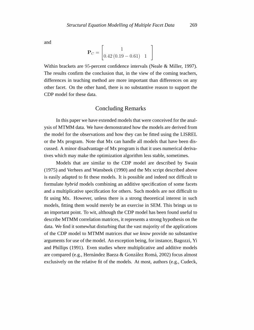
Structural Equation Modelling of Multiple Facet Data 269
and
PC =
[1
0.42 (0.19− 0.61) 1
]Within brackets are95-percent confidence intervals (Neale & Miller, 1997).
The results confirm the conclusion that, in the view of the coming teachers,
differences in teaching method are more important than differences on any
other facet. On the other hand, there is no substantive reason to support the
CDP model for these data.
Concluding Remarks
In this paper we have extended models that were conceived for the anal-
ysis of MTMM data. We have demonstrated how the models are derived from
the model for the observations and how they can be fitted using the LISREL
or the Mx program. Note that Mx can handle all models that have been dis-
cussed. A minor disadvantage of Mx program is that it uses numerical deriva-
tives which may make the optimization algorithm less stable, sometimes.
Models that are similar to the CDP model are described by Swain
(1975) and Verhees and Wansbeek (1990) and the Mx script described above
is easily adapted to fit these models. It is possible and indeed not difficult to
formulatehybrid models combining an additive specification of some facets
and a multiplicative specification for others. Such models are not difficult to
fit using Mx. However, unless there is a strong theoretical interest in such
models, fitting them would merely be an exercise in SEM. This brings us to
an important point. To wit, although the CDP model has been found useful to
describe MTMM correlation matrices, it represents a strong hypothesis on the
data. We find it somewhat disturbing that the vast majority of the applications
of the CDP model to MTMM matricesthat we knowprovide no substantive
arguments for use of the model. An exception being, for instance, Bagozzi, Yi
and Phillips (1991). Even studies where multiplicative and additive models
are compared (e.g., Hernandez Baeza & Gonzalez Roma, 2002) focus almost
exclusively on the relative fit of the models. At most, authors (e.g., Cudeck,

270 T.M. Bechger and G. Maris
1988, p. 141) refer to the work by Campbell and O’Connell (1967; 1982)
who observed that for some MTMM correlation matrices, inter-trait correla-
tions are attenuated by a multiplicative constant (smaller in magnitude than
unity), when different methods are used.
In closing, we mention two topics for future research. First, it is nec-
essary to establish the identifiability of the (reparameterized) CC and CDP
model. Although we believe these models to be identifiable there is no general
proof available that they are identifiable for any number of facets. Second, we
would like to have ways to perform exploratory analysis on the within-facet
covariance (or correlation) matrices. A suggestion is to use a model incor-
porating principal components. Such model have been considered (for two-
facets) by Flury and Neuenschwander (1995). Dolan, Bechger, and Molenaar
(1999) suggest how these model can be fitted in a SEM framework.
Structural Equation Modelling of Multiple Facet Data 271
REFERENCES
Bagozzi, R. P., Yi, Y. & Phillips, L. W. (1991). Assessing construct validity in organizationalresearch.Administrative Science Quarterly, 36, 421-458.
Bagozzi, R. P., Yi, Y., & Nassen, K. D. (1999). Representation of measurement error in mar-keting variables: Review of approaches and extension to three-facet designs.Journal ofEconometrics, 89, 393-421.
Bechger, T. M., Verhelst, N. D., & Verstralen, H. H. F. M. (2001). Identifiability of nonlinearlogistic test models.Psychometrika, 66, 357-372
Bock, R. D., & Bargmann, R. E. (1966). Analysis of covariance structures.Psychometrika, 31(4),507-534.
Bollen, K. A. (1989).Structural Equations with Latent Variables.New York: Wiley.Browne, M. W. (1970).Analysis of covariance structures.Paper presented at the annual confer-
ence of the South African Statistical Association.Browne, M. W. (1984). The decomposition of multitrait-multimethod matrices.British Journal of
Mathematical and Statistical Psychology, 37, 1-21.Browne, M. W. (1989). Relationships between an additive model and a multiplicative model for
multitrait-multimethod matrices. In R. Coppi & S. Bolasco. (Eds.).Multiway Data Analysis.New-York: Elsevier.
Browne, M. W. (1993). Models for Multitrait Multimethod Matrices. in R Steyer, K. F. Wenders& Widaman, K.F. (Eds.)Psychometric Methodology. Proceedings of the 7th EuropeanMeeting of the Psychometric Society in Trier. (pp. 61-73) New York : Fisher.
Browne, M. W., & Strydom, H. F. (1997). Non-iterative fitting of the direct product model formultitrait-multimethod matrices. In M. Berkane (Editor).Latent variable modeling andapplications to causality. New-York: Springer.
Campbell, D. T., & Fiske, D. W. (1959). Convergent and discriminant validation by the multitrait-multimethod matrix.Psychological Bulletin, 56, 81-105.
Campbell, D. T., & O’Connell, E. J. (1967). Method factors in multitrait-multimethod matrices:Multiplicative rather than additive?Multivariate Behavioral Research, 2, 409-426.
Campbell, D. T., & O’Connell, E. J. (1982). Methods as diluting trait relationships rather thanadding irrelevant systematic variance. In D. Brinberg and L.H. Kidder (Eds.)Forms ofvalidity in research. New directions for methodology of social and behavioral science. Vol.12.
Cudeck, R. (1988). Multiplicative Models and MTMM matrices.Journal of Educational Statis-tics, 13(2), 131-147.
Cudeck, R. (1989). Analysis of correlation matrices using covariance structure models.Psycho-logical Bulletin, 105(2), 317-327.
Dolan, C. V. , Bechger, T. M., & Molenaar, P. C. M. (1999). Fitting models incorporating principalcomponents using LISREL 8.Structural Equation Modeling, 6(3), 233-261.
Fiske, D. W. (1971).Measuring the concepts of intelligence. Chicago: Aldine.
272 T.M. Bechger and G. Maris
Flury, B. D., & Neuenschwander, B. E. (1995). Principal component models for patterned covari-ance matrices with applications to canonical correlation analysis of several sets of variables.Chapter 5 In W.J. Krzanowski (Ed.)Recent Advances in Descriptive Multivariate Analysis,Oxford: Oxford University Press.
Guilford, J. P. (1967).The nature of human intelligence. New-York: McGraw-Hill.Hernandez Baeza, A., & Gonzalez Roma, V. (2002). Analysis of Multitrait-Multioccasion Data:
Additive versus Multiplicative Models.Multivariate Behavioral Research, 37(1), 59-87.Hilton, T. L., Beaton, A. E., & Bower, C. P. (1971).Stability and instability in academic growth:
A compilation of longitudinal data. Final report, USOE, Research No 0-0140. Princeton,NJ: ETS.
Hoeks, J. (1985).Vaardigheden in begrijpend lezen. [Abilities in reading comprehension]. Un-published dissertation, University of Amsterdam.
Hoeks, J., Mellenbergh, G. J., & Molenaar, P. C. M. (1989)Fitting linear models to semantic testsconstructed according to Guilford’s facet design.University of Amsterdam.
Joreskog, K. G. (1973). Analyzing psychological data by structural analysis of covariance ma-trices. In D.H. Krantz, R.D. Luce., R.C. Atkinson & P. Suppes (Eds.)Measurement, psy-chophysics and neural information processing.Volume II of Contemporary developmentsin mathematical Psychology. San Fransisco: W.H. Freeman and Company.
Joreskog, K. G. , & Sorbom, D. (1996).LISREL8 User’s reference Guide. SSI.McDonald, R. P. (1989). An index of goodness-of-fit based on noncentrality.Journal of Classifi-
cation, 6, 97-103.Neale, M. C. , Boker, S. M. , Xie, G., & Maes, H. (2002).Mx: Statistical modelling. Virginia
Institute for Psychiatric and Behavioral Genetics, Virgina Commonwealth University, De-partment of Psychiatry.
Neale, M. C. , & Miller, M. B. (1997). The use of likelihood-based confidence intervals in geneticmodels.Behaviour Genetics, 20, 287-298.
Pringle, R. M., & Rayner, A. A. (1971).Generalized inverse matrices with applications to statis-tics. London: Griffin.
Steiger, J. H., Lind, J. C. (1980).Statistically-based tests for the number of common factors.Paperpresented at the annual Spring Meeting of the Psychometric Society in Iowa City.
Swain, A. J. (1975).Analysis of Parametric Structures for Covariance Matrices. UnpublishedPhD thesis. University of Adelaide.
Verhees, J. , & Wansbeek, T. J. (1990). A multimode direct product model for covariance structureanalysis.British Journal of Mathematical and Statistical Psychology, 43, 231-240.
Wiley, D., Schmidt, W. H., & Bramble, W. J. (1973). Studies of a class of covariance structuremodels.Journal of the American statistical association, 68(342), 317-323.
Wothke, W. (1984).The estimation of trait and method components in multitrait multimethodmeasurement. University of Chigago, Department of Behavioral Science: Unpublisheddissertation.
Wothke, W. (1988).Identification conditions for scale-free covariance component models.PaperPresented at the Annual Meeting of the Psychometric Society, Los Angeles, June 26-29.
Wothke, W. (1996). Models for multitrait-multimethod matrix analysis. Chapter 2 inAdvancedtechniques for structural equation modeling, Edited by R.E. Schumacker and G.A. Mar-coulides. New-York: Lawrence Erlbaum Associates.
Wothke, W., & Browne, M. W. (1990). The direct product model for the MTMM matrix parame-terized as a second order factor analysis model.Psychometrika, 55, 255-262.

Structural Equation Modelling of Multiple Facet Data 273
Appendix
TItle Hoeks data CC model on correlationsDa No=620 Ni=18KM SY1.0000.502 1.00000.512 0.475 1.00000.419 0.313 0.419 1.0000.457 0.457 0.430 0.385 1.0000.481 0.401 0.479 0.431 0.405 1.0000.568 0.519 0.530 0.501 0.553 0.497 1.0000.456 0.396 0.494 0.512 0.491 0.449 0.637 1.0000.527 0.470 0.444 0.453 0.490 0.491 0.680 0.675 1.0000.485 0.433 0.418 0.373 0.415 0.361 0.544 0.425 0.533 1.0000.426 0.388 0.392 0.384 0.407 0.339 0.445 0.413 0.436 0.4411.0000.293 0.282 0.306 0.259 0.262 0.253 0.290 0.222 0.271 0.2730.243 1.0000.573 0.508 0.577 0.487 0.482 0.516 0.642 0.555 0.558 0.5160.404 0.303 1.0000.516 0.389 0.465 0.390 0.420 0.436 0.517 0.456 0.461 0.4340.348 0.286 0.582 1.0000.497 0.398 0.410 0.445 0.452 0.483 0.616 0.572 0.598 0.5520.401 0.247 0.601 0.494 1.0000.160 0.101 0.212 0.151 0.093 0.256 0.152 0.196 0.156 0.1860.117 0.137 0.166 0.119 0.159 1.0000.206 0.106 0.140 0.162 0.204 0.239 0.131 0.103 0.073 0.1700.178 0.333 0.215 0.288 0.207 0.106 1.0000.251 0.168 0.226 0.233 0.250 0.378 0.248 0.229 0.221 0.2500.169 0.272 0.293 0.267 0.276 0.440 0.290 1.000mo ny=18 ne=18 nk=4 ps=ze,fi ly=di,fr ga=fu,fi ph=sy,frMA gamma1 0 0 0 !0 01 0 0 0 !1 01 0 0 0 !0 11 0 0 0 !0 01 0 0 0 !1 01 0 0 0 !0 11 0 1 0 !0 0

274 T.M. Bechger and G. Maris
1 0 1 0 !1 01 0 1 0 !0 11 1 1 0 !0 01 1 1 0 !1 01 1 1 0 !0 11 1 0 1 !0 01 1 0 1 !1 01 1 0 1 !0 11 1 0 1 !0 01 1 0 1 !1 01 1 0 1 !0 1pa ph00 10 0 10 0 0 1!0 0 0 0 1!0 0 0 0 1 1va 1 ph(1,1)st 0.3 allou se rs ULS it=40000
Note that anything after a ! is ignored by LISREL. We have kept it here to illustratehow the script was changed from the first to the final analysis.