1. A time series is a:

A) set of measurements on a variable collected at the same time or approximately the same period of time.

B) is a set of measurements, ordered over time, on a particular quantity of interest.C) model that attempts to analyze the relationship between a dependent variable and one

or more independent variables.D) model that attempts to forecast the future value of a variable.ANSWER: B

2. Which of the following components in the time series is more likely to exhibit the relative steady growth of the population of Egypt from 1959 to 2009?

A) the trend componentB) the cyclical componentC) the seasonal componentD) the irregular componentANSWER: A

3. The exponential smoothing method of forecasting is the most appropriate method for time series that exhibit:

A) irregularity.B) seasonality.C) a constant upward trend.D) a constant downward trend.ANSWER: A

4. The time series that reflects a wavelike pattern describing a long-term trend that is generally apparent over a number of years is called the ____.

A) trend component B) cyclical componentC) seasonal componentD) irregular componentANSWER: B

5. We calculate the three-period moving averages for a time series for all time periods except the:

A) first period.B) last period.C) first and last period.D) first and last two periods.ANSWER: C

6. We calculate the five-period moving average for a time series for all time periods except the:

A) first five periods.B) last five periods.C) first and last period.D) first two and last two periods.ANSWER: D

7. The component in a time series that reflects a long-term, relatively smooth pattern or direction exhibited by a time series over a long time period (more than one year) is called the ____.

A) trend component B) cyclical componentC) seasonal componentD) irregular componentANSWER: A

8. The number of four-period centered moving averages of a time series with 20 time periods is ____.

A) 28B) 24C) 20D) 16ANSWER: D

9. Seasonality is a time-series component.ANSWER: T

10. The choice of a larger smoothing constant in simple exponential smoothing would place more weight on the most recent value.ANSWER: TCourse LO: Discuss the applications of time-series forecasting, trend models, and qualitative approaches

11. The formula that explains simple exponential smoothing is for 0 < < 1.ANSWER: T

12. Simple exponential smoothing provides a forecast based on a weighted average of current and past values.ANSWER: T

13. The seasonal component in a time series reflects a long-term, relatively smooth pattern or direction.ANSWER: F

14. We calculate the three-period moving average for a time series for all time periods except the first period.ANSWER: F

15. The term seasonal variation may refer to the four traditional seasons, or to systematic patterns that occur during a month, a week, or even one day.

16. Given a data set with 20 yearly observations, there are only twelve 9-year moving averages.ANSWER: T

17. The irregular component of a time series exhibits a tendency to grow or decrease rather steadily over long periods of time.ANSWER: F

18. Increasing the value of from 0.025 to 0.10 in exponential smoothing will increase the weight to the most recent observation by 0.075.ANSWER: F

19. If we could characterize time series primarily in terms of trend, seasonal, and cyclical components, then the series would vary smoothly over time, and forecasts could be made using these components.ANSWER: T

THE NEXT SIX QUESTIONS ARE BASED ON THE FOLLOWING INFORMATION: Very Important

The table below is the data set of the Shiller Real Home Price Index for the years 1934-1944.

Year Real Home Price Index

1934 73.27941113

1935 78.06999903

1936 79.41489505

1937 79.71761781

1938 78.46465294

1939 78.54968493

1940 81.73080633

1941 73.81588343

1942 68.50282683

1943 70.9229742

1944 80.30899579

20. If the forecaster uses an exponential smoothing constant of 0.8, show the steps involved in calculating the forecast for the year 1935.

ANSWER:

The process begins by setting the first element of the series:

The second value which is the forecast for the year 1935 is then

.

21. Use a smoothing constant of 0.8 to show the table that shows all the forecast values for the given series.

ANSWER:

The process begins by setting the first element of the series:

The second value in the forecast is then .

The third value in the forecast is then .

Follow the same procedure to calculate the other forecast values.

Year Real Home Price Index

1934 73.27941113 73.27941

1935 78.06999903 77.11188

1936 79.41489505 78.95429

1937 79.71761781 79.56495

1938 78.46465294 78.68471

1939 78.54968493 78.57669

1940 81.73080633 81.09998

1941 73.81588343 75.2727

1942 68.50282683 69.8568

1943 70.9229742 70.70974

1944 80.30899579 78.38914

22. Assuming a smoothing constant of 0.8, find the error term for the year 1936.

ANSWER:

The process begins by setting the first element of the series

The second value in the forecast is then .

The third value in the forecast is then .

The error term for the third year: .

23. Use a smoothing constant of 0.8 to show the table that shows all the error terms for the given series.

ANSWER:

The process begins by setting the first element of the series:

The second value in the forecast is then .

The third value in the forecast is then .

Follow the same procedure to calculate the other forecast values.

Therefore, the error term for the third year: .

Follow the same procedure to determine the other error terms.

Year Real Home Price Index

1934 73.27941113 73.27941 0

1935 78.06999903 77.11188 4.7905879

1936 79.41489505 78.95429 2.303013601

1937 79.71761781 79.56495 0.763325478

1938 78.46465294 78.68471 –1.100299775

1939 78.54968493 78.57669 –0.135027957

1940 81.73080633 81.09998 3.154115802

1941 73.81588343 75.2727 –7.284099738

1942 68.50282683 69.8568 –6.769876548

1943 70.9229742 70.70974 1.066172062

1944 80.30899579 78.38914 9.599255998

24. Show the calculations of the sum of squared errors.

ANSWER:

The process begins by setting the first element of the series:

The second value in the forecast is then .

The third value in the forecast is then .

Follow the same procedure to calculate the other forecast values.

The error term for the third year: .

Follow the same procedure to determine the other error terms.

Square all the error terms and find the sum.

Year Real Home Price Index

1934 73.27941113

73.27941 0 0

1935 78.06999903

77.11188 4.7905879

22.94973243

1936 79.41489505

78.95429 2.303013601

5.303871645

1937 79.71761781

79.56495 0.763325478

0.582665785

1938 78.46465294

78.68471

–1.100299775

1.210659594

1939 78.54968493

78.57669

–0.135027957

0.018232549

1940 81.73080633

81.09998 3.154115802

9.948446491

1941 73.81588343 75.2727

–7.284099738 53.058109

1942 68.50282683 69.8568

–6.769876548

45.83122848

1943 70.9229742

70.70974 1.066172062

1.136722867

1944 80.30899579

78.38914 9.599255998

92.14571572

SS = = 232.19

25. What is the forecast for the year 1945 if its real home price index is 98.056?

ANSWER:

Year Real Home Price Index

1934 73.27941113 73.27941

1935 78.06999903 77.11188

1936 79.41489505 78.95429

1937 79.71761781 79.56495

1938 78.46465294 78.68471

1939 78.54968493 78.57669

1940 81.73080633 81.09998

1941 73.81588343 75.2727

1942 68.50282683 69.8568

1943 70.9229742 70.70974

1944 80.30899579 78.38914

For the year 1945,

26. Identify the four components of a time series.

ANSWER:

A time series contains four components: the trend component, the seasonal

component, the cyclical component, and the irregular component.

27. Consider the following time-series data. Develop the simple centered 5-point moving average for this series.

Period xt

1 35

2 24

3 41

4 38

5 31

6 28

7 27

8 30

9 49

10 40

11 35

12 44

ANSWER:

28. The table below shows the weekly sales of umbrellas during the rainy season. How will you go about removing the irregularity component of this time series using the method of 4-point moving averages?

Week Sales

1 100

2 113

3 119

4 124

5 125

6 131

7 133

8 144

Period xt MA

1 35 *

2 24 *

3 41 33.8

4 38 32.4

5 31 33.0

6 28 30.8

7 27 33.0

8 30 34.8

9 49 36.2

10 40 39.6

11 35 *

12 44 *

9 147

10 151

ANSWER:

To remove the irregularity component, the 4-point moving averages and the respective 4-point centered moving averages are calculated.

4-point moving averages:

Similarly, are calculated.

Centered 4-point moving averages:

Similarly, are calculated.

The table shows the calculated values.

Week Sales4-point moving

averagesCentered 4-point moving averages

1 100

2 113

114

3 119 117.125

120.25

4 124 122.5

124.75

5 125 126.5

128.25

6 131 130.75

133.25

7 133 136

138.75

8 144 141.25

143.75

9 147

10 151

THE NEXT THREE QUESTIONS ARE BASED ON THE FOLLOWING INFORMATION : Very Important Math

The table below shows the corporate earnings percentage of an enterprise for 5 years.The company’s forecaster uses the 4-period centered moving average to remove the seasonality component.

YearQuarter xt

1.1 0.8

1.2 0.72

1.3 0.9

1.4 1.62

2.1 0.86

2.2 1.308

2.3 0.88

2.4 2.13

3.1 2.57

3.2 0.9

3.3 1.283

3.4 2.566

4.1 3.26

4.2 1.64

4.3 1.02

4.4 1.05

5.1 2.1

5.2 1.6

5.3 2.7

5.4 1.6

29. How will you go about removing the irregularity component of this time series using the method of 4-point moving averages?

ANSWER:

To remove the irregularity component, the 4-point moving averages and the respective 4-point centered moving averages are calculated.

4-point moving averages:

Similarly,

are calculated.

Centered 4-point moving averages:

Similarly, are calculated.

The table shows the calculated values.

YearQuarter

xt 4-point moving averages

Centered 4-point moving averages1.1 0.8

1.2 0.72

1.01

1.3 0.9 1.0175

1.025

1.4 1.62 1.0985

1.172

2.1 0.86 1.1695

1.167

2.2 1.308 1.23075

1.2945

2.3 0.88 1.50825

1.722

2.4 2.13 1.671

1.62

3.1 2.57 1.670375

1.72075

3.2 0.9 1.77525

1.82975

3.3 1.283 1.916

2.00225

3.4 2.566 2.09475

2.18725

4.1 3.26 2.154375

2.1215

4.2 1.64 1.932

1.7425

4.3 1.02 1.5975

1.4525

4.4 1.05 1.4475

1.4425

5.1 2.1 1.6525

1.8625

5.2 1.6 1.93125

2

5.3 2.7

5.4 1.6

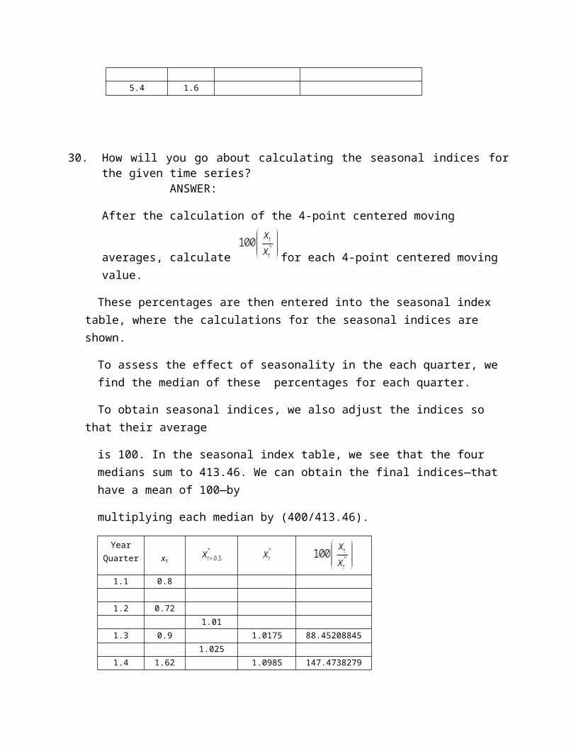
30. How will you go about calculating the seasonal indices for the given time series?ANSWER:

After the calculation of the 4-point centered moving averages, calculate for each 4-point centered moving value.

These percentages are then entered into the seasonal index table, where the calculations for the seasonal indices are shown.

To assess the effect of seasonality in the each quarter, we find the median of these percentages for each quarter.

To obtain seasonal indices, we also adjust the indices so that their average

is 100. In the seasonal index table, we see that the four medians sum to 413.46. We can obtain the final indices—that have a mean of 100—by

multiplying each median by (400/413.46).

YearQuarter xt

1.1 0.8

1.2 0.72

1.01

1.3 0.9 1.0175 88.45208845

1.025

1.4 1.62 1.0985 147.4738279

1.172

2.1 0.86 1.1695 73.53569902

1.167

2.2 1.308 1.23075 106.2766606

1.2945

2.3 0.88 1.50825 58.34576496

1.722

2.4 2.13 1.671 127.4685817

1.62

3.1 2.57 1.670375 153.8576667

1.72075

3.2 0.9 1.77525 50.69708492

1.82975

3.3 1.283 1.916 66.96242171

2.00225

3.4 2.566 2.09475 122.496718

2.18725

4.1 3.26 2.154375 151.3199884

2.1215

4.2 1.64 1.932 84.88612836

1.7425

4.3 1.02 1.5975 63.84976526

1.4525

4.4 1.05 1.4475 72.5388601

1.4425

5.1 2.1 1.6525 127.0801815

1.8625

5.2 1.6 1.93125 82.84789644

2

5.3 2.7

5.4 1.6

Seasonal Index Table:

Year\Quarter 1 2 3 4 SUM

1 88.45147.4

7

2 73.54 106.28 58.35 127.4

7

3 153.86 50.70 66.96122.5

0

4 151.32 84.89 63.85 72.54

5 127.08 82.85

MEDIAN 139.20 83.87 65.41124.9

8 413.46

Seasonal Index 134.67 81.14 63.28120.9

2 400

Difficulty: 3 Challenging

Topic: Moving Averages

AACSB: Analytic Skills

Course LO: Discuss the applications of time-series forecasting, trend models, and qualitative approaches

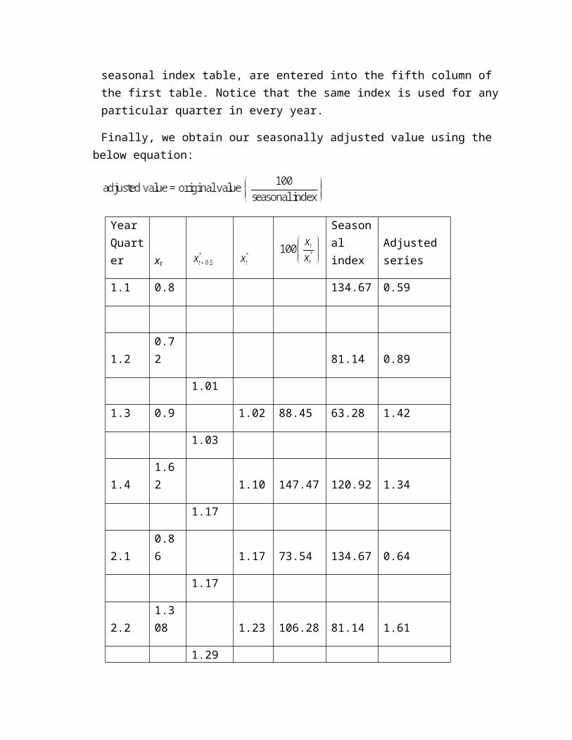
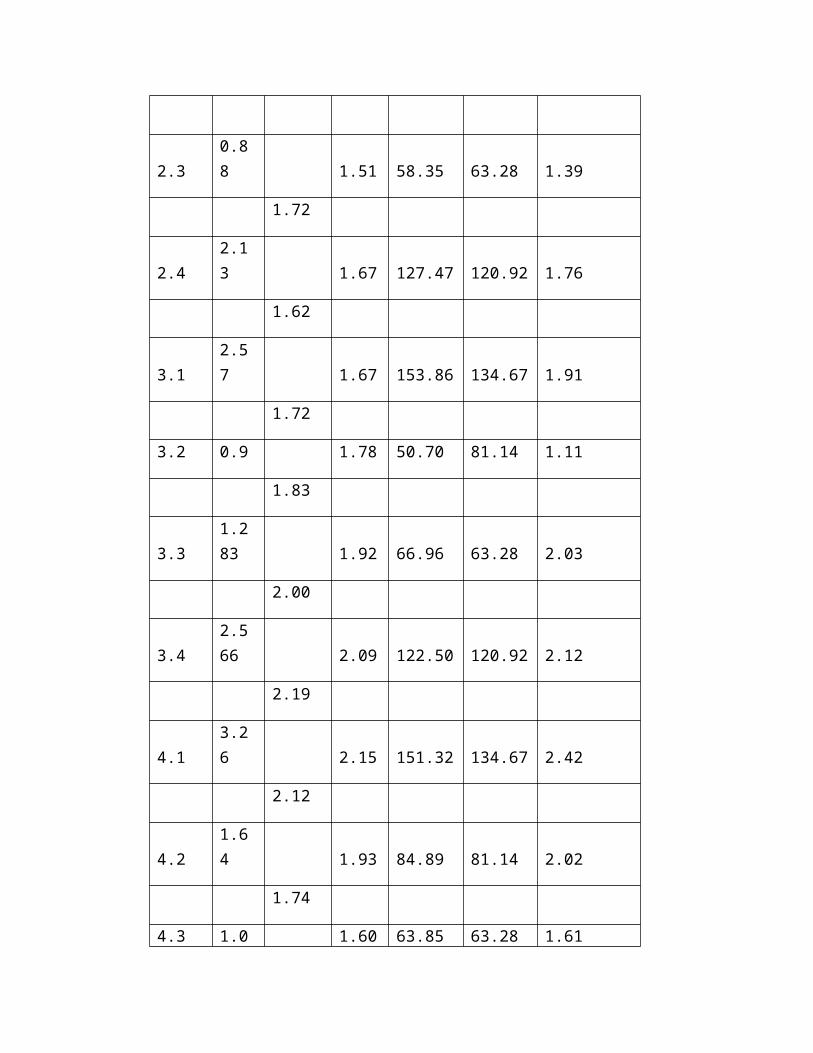
31. How do you remove the seasonality component from the given time series.

ANSWER:

Once the seasonal indices for all the quarters are calculated, these seasonal indices, from the last row of the seasonal index table, are entered into the fifth column of the first table. Notice that the same index is used for any particular quarter in every year.

Finally, we obtain our seasonally adjusted value using the below equation:

YearQuarter xt

Seasonal index

Adjusted series

1.1 0.8 134.67 0.59

1.2 0.72 81.14 0.89

1.01

1.3 0.9 1.02 88.45 63.28 1.42

1.03

1.4 1.62 1.10 147.47 120.92 1.34

1.17

2.1 0.86 1.17 73.54 134.67 0.64

1.17

2.2 1.308 1.23 106.28 81.14 1.61

1.29

2.3 0.88 1.51 58.35 63.28 1.39

1.72

2.4 2.13 1.67 127.47 120.92 1.76

1.62

3.1 2.57 1.67 153.86 134.67 1.91

1.72

3.2 0.9 1.78 50.70 81.14 1.11

1.83

3.3 1.283 1.92 66.96 63.28 2.03

2.00

3.4 2.566 2.09 122.50 120.92 2.12

2.19

4.1 3.26 2.15 151.32 134.67 2.42

2.12

4.2 1.64 1.93 84.89 81.14 2.02

1.74

4.3 1.02 1.60 63.85 63.28 1.61

1.45

4.4 1.05 1.45 72.54 120.92 0.87

1.44

5.1 2.1 1.65 127.08 134.67 1.56

1.86

5.2 1.6 1.93 82.85 81.14 1.97

2.00

5.3 2.7 63.28 4.27

5.4 1.6 120.92 1.32

Seasonal Index Table:

Year\Quarter 1 2 3 4 SUM

1 88.45 147.47

2 73.54106.2

8 58.35 127.47

3 153.86 50.70 66.96 122.50

4 151.32 84.89 63.85 72.54

5 127.08 82.85

MEDIAN 139.20 83.87 65.41 124.98 413.46

Seasonal Index 134.67 81.14 63.28 120.92 400

THE NEXT ELEVEN QUESTIONS ARE BASED ON THE FOLLOWING INFORMATION:

The table below is the data set of the number of preorders received for a particular game on a weekly basis.The forecaster uses the Holt-Winters Exponential Smoothing for nonseasonal series to forecast the number of preorders in future time periods.He uses = 0.8 and = 0.5. (Hint: Use the formula from the text to arrive at the answers.)

WeekPreorder

s

1 266

2 310

3 330

4 342

5 388

6 462

7 548

8 624

9 666

10 686

11 726

32. What is initial estimate of the trend value for week 2?

A) 34B) 24C) 44D) 43ANSWER: C

33. The trend estimate for ____ is 49 approximately.

A) week 6B) week 4

C) week 8D) week 2ANSWER: A

34. Which of the following weeks has an approximate trend estimate of 68?

A) week 5B) week 7C) week 1D) week 11ANSWER: B

35. What is the trend estimate for week 10?

A) 38.18B) 34.40C) 43.48D) 50.00ANSWER: C

36. The estimate of the level for week 2 is ____.

A) 452 unitsB) 347 unitsC) 335 unitsD) 310 unitsANSWER: D

37. What is the approximate level estimate for week 8?

A) 453 unitsB) 539 unitsC) 620 unitsD) 696 unitsANSWER: C

38. The estimate of the level for ____ is 453 units, approximately.

A) week 6B) week 4C) week 5D) week 8ANSWER: A

39. Which of the following weeks has a level estimate of 672 units approximately?

A) week 5B) week 7C) week 9D) week 13ANSWER: C

40. Compute the approximate forecast for week 12.

A) 696 unitsB) 767 unitsC) 672 unitsD) 453 unitsANSWER: B

41. The forecast for week 13 is approximately ____.

A) 696 unitsB) 767 unitsC) 805 unitsD) 966 unitsANSWER: C

42. What is the approximate forecast for week 14?

A) 843 unitsB) 348 unitsC) 483 unitsD) 438 unitsANSWER: ADifficulty: 2 Moderate

43. In which component of the time series will the effect of an unpredictable, rare event be contained?

A) the trend componentB) the seasonal componentC) the cyclical componentD) the irregular componentANSWER: D

44. The time-series model is used for forecasting, where and are respectively the trend, seasonal, cyclical, and irregular components of the time series,

and is the value of the time series at time t. The following estimates are obtained:

The model will produce a forecast of ____.

A) 127.86B) 122.14C) 107.64D) 102.99ANSWER: C